Second-order chiral kinetic theory: Chiral magnetic and pseudomagnetic waves

Abstract

The consistent chiral kinetic theory accurate to the second order in electromagnetic and pseudoelectromagnetic fields is derived for a relativistic matter with two Weyl fermions. By making use of such a framework, the properties of longitudinal collective excitations, which include both chiral magnetic and chiral pseudomagnetic waves, are studied. It is shown that the proper treatment of dynamical electromagnetism transforms these gapless waves into chiral (pseudo)magnetic plasmons, whose Langmuir (plasma) gap receives corrections quadratic in both magnetic and pseudomagnetic fields.

I Introduction

A kinetic theory is a common framework for studying a wide range of physical properties in condensed matter materials, nuclear physics, and cosmology Landau:t10 ; Krall . A relativistic version of such a theory is invaluable in studies of numerous relativistic forms of matter, e.g., realized in the primordial plasma of the early universe Kronberg ; Durrer , relativistic heavy-ion collisions Kharzeev:2008-Nucl ; Kharzeev:2016 , compact stars Kouveliotou:1999 , as well as the Dirac and Weyl materials. Following the first theoretical predictions in Refs. Wang ; Weng ; Weng:2014 , the realization of the three-dimensional (3D) Dirac semimetal phase in A₃Bi ($\mathrm{A=Na,K,Rb}$), Cd₃As₂, and ZrTe₅ was confirmed experimentally Borisenko ; Neupane ; Liu ; Xiong:2015 ; Li-Wang:2015 ; Li-He:2015 ; Li:2014bha ; Zheng:2016 . While the Weyl semimetal phase was first predicted theoretically to be realized in pyrochlore iridates Savrasov , it was discovered later in such compounds as $\mathrm{TaAs}$, $\mathrm{TaP}$, $\mathrm{NbAs}$, $\mathrm{NbP}$, $\mathrm{Mo_{x}W_{1-x}Te}$, and $\mathrm{YbMnBi_{2}}$ Weng-Fang:2015 ; Qian ; Huang:2015eia ; Bian ; Huang:2015Nature ; Zhang:2016 ; Cava ; Belopolski . The above-mentioned forms of matter are often made of (approximately) massless fermionic particles that carry a well-defined chirality. Therefore, the chirality could be treated as a natural additional degree of freedom in a relativistic plasma. It should be noted, however, that the conservation of the chiral charge is violated in the presence of external electromagnetic fields. This is a consequence of the celebrated chiral (triangle) anomaly ABJ . Nevertheless, this anomaly can be incorporated exactly in the chiral kinetic theory Son:2012wh ; Stephanov:2012ki . The only limitation of the current formulation of the corresponding theory is that it is valid only to the linear order in electromagnetic fields.

It important to note that the chiral anomaly affects magnetotransport in Weyl and Dirac semimetals in a nontrivial way. Indeed, as was first shown by Nielsen and Ninomiya Nielsen , the longitudinal (with respect to the direction of an external magnetic field) magnetoresistivity in Weyl semimetals decreases with the growth of the magnetic field. Physically this phenomenon, which is usually called negative magnetoresistivity, relies on the presence of the lowest Landau level (LLL) states around each Weyl node Nielsen ; Son . Then, since the LLL density of states grows linearly with a magnetic field, the conductivity increases too. The phenomenon of negative magnetoresistivity is extensively studied both theoretically Nielsen ; Son ; Aji:2012 ; Kim:2013dia ; Gorbar:2013dha ; Burkov:2015 and experimentally Li:2014bha ; Xiong:2015 ; Li-He:2015 ; Li-Wang:2015 ; Huang:2015eia ; Zhang:2016 .

The presence of a chiral chemical potential $\mu_{5}$, which quantifies a chiral asymmetry in a relativistic matter, significantly enriches the properties and types of collective excitations. The investigation of the corresponding features began in Refs. Kharzeev:2010gd ; Akamatsu:2013 ; Stephanov:2015 . The authors of Ref. Kharzeev:2010gd showed that the triangle anomaly implies the existence of a novel type of collective excitations which stems from the coupling between the density waves of the electric and chiral charges and is known as the chiral magnetic wave (CMW). In this connection, let us also mention that, as was shown in Ref. Akamatsu:2013 , a nonzero chiral chemical potential lifts the degeneracy of the transverse plasma modes, but leaves the longitudinal mode intact. Such a conclusion agrees with a refined analysis in the consistent chiral kinetic theory Gorbar:2016ygi ; Gorbar:2016sey .

Dirac and Weyl materials provide additional opportunities to explore the role of chirality. For example, they allow for a simple realization of axial electric (or pseudoelectric) $\mathbf{E}_{5}$ and/or axial magnetic (or pseudomagnetic) $\mathbf{B}_{5}$ fields. These pseudoelectromagnetic fields act on fermions as ordinary electromagnetic fields, but their sign depends on the fermion chirality. In Weyl and Dirac materials, one can induce a background pseudomagnetic field $\mathbf{B}_{5}$ by various kinds of static strains Zubkov:2015 ; Cortijo:2016yph ; Pikulin:2016 ; Cortijo:2016 ; Grushin-Vishwanath:2016 ; Liu-Pikulin:2016 . Note that, unlike an ordinary magnetic field $\mathbf{B}$, a pseudomagnetic one does not break the time-reversal symmetry. In essence, this is due to the fact that Weyl nodes in condensed matter materials always come in pairs of opposite chirality Nielsen:1980rz . A pseudoelectric $\mathbf{E}_{5}$ can be induced by time-dependent strains Pikulin:2016 .

Recently, we showed Gorbar:2016ygi ; Gorbar:2016sey that the plasmons in a relativistic matter in constant magnetic and pseudomagnetic fields are, in fact, chiral (pseudo)magnetic plasmons. Their chiral nature is manifested by oscillations of a chiral charge density, which are absent for ordinary electromagnetic plasmons. It is also worth noting that, in the presence of magnetic fields, the quasiparticle plasma in uncompensated metals supports a special type of collective excitations known as helicons. These transverse low-energy gapless excitations propagate along the background magnetic field. According to the studies in Ref. Pellegrino , the dispersion relation of helicons encodes information on the chiral shift parameter $\mathbf{b}$, which defines the momentum space separation of Weyl nodes. Further, by using the formalism of the consistent chiral kinetic theory, it was shown in Ref. Gorbar:2016vvg that pseudomagnetic fields allow for a new type of helicons, which we called pseudomagnetic helicons.

Although the chiral kinetic theory is quite successful in the description of various processes in relativistic plasma, many physical phenomena require its formulation accurate to the second order in electromagnetic fields. Recently, using the wave-packet semiclassical approach Sundaram:1999zz (for a review, see Ref. Xiao:2009rm ), all the necessary ingredients for such a formulation were provided in Refs. Gao:2014 ; Gao:2015 for condensed matter systems with a general band structure. In the present paper, we derive the explicit expressions for the consistent chiral kinetic theory valid to the second order in electromagnetic, as well as pseudoelectromagnetic fields for a simple realization of relativistic matter in a Weyl material with a single pair of Weyl nodes.

The effects of dynamical electromagnetism for the chiral magnetic and chiral pseudomagnetic waves were studied in Ref. Gorbar:2016sey in the consistent chiral kinetic theory valid to the linear order in electromagnetic and pseudoelectromagnetic fields. It was found that such excitations are chiral (pseudo)magnetic plasmons with the field-independent Langmuir (plasma) gap. While the background magnetic field does not affect at all the dispersion relation in the linear order, the background pseudomagnetic field contributes only to the term linear in momentum. However, according to the general arguments in Ref. Kharzeev:2010gd , the dispersion relation of the CMW with the effects of dynamical electromagnetism included should have the form $\omega^{2}=\Omega^{2}_{e}+(v^{2}_{\chi}+c^{2}_{\rm eff})\mathbf{k}^{2}$, where $v_{\chi}\propto eB$. Since $v^{2}_{\chi}$ is proportional to the square of the magnetic field, this result cannot be reliably reproduced in the conventional first-order chiral kinetic theory Son:2012wh ; Stephanov:2012ki , unless the theory is generalized to the second order in electromagnetic fields. In essence, this is one of the main motivations for this paper.

The paper is organized as follows. The consistent chiral kinetic theory for a Weyl material with two Weyl fermions valid to the second order in electromagnetic and pseudoelectromagnetic fields is formulated in Sec. II. The longitudinal collective excitations propagating along background magnetic and pseudomagnetic fields are considered in Sec. III. The summary of the main results is given in Sec. IV. Some useful technical results and formulas are presented in Appendixes A and B.

II Second-order chiral kinetic theory

Let us start by discussing the form of the second order in electromagnetic and pseudoelectromagnetic field corrections to the quasiparticle energy and velocity, as well as the leading-order corrections to the Berry curvature. (Indeed, the first-order corrections to the Berry curvature are sufficient because in the chiral kinetic theory it always couples to electromagnetic fields Gao:2014 ; Gao:2015 .) Our starting point is the Hamiltonian for a single Weyl fermion

$$H=\lambda v_{F}(\mathbf{p}\cdot\bm{\sigma}),$$ (1)

where $\lambda=\pm$ is chirality, $v_{F}$ is the Fermi velocity, $\mathbf{p}$ is a momentum, and $\bm{\sigma}$ are the Pauli matrices. In the absence of external electromagnetic fields, the quasiparticle energy is $\epsilon^{(0)}_{\eta}=\eta v_{F}p$, where $\eta$ labels the quasiparticles in the upper ($\eta=+1$) or lower ($\eta=-1$) band. (Note that in relativistic language, the quasiparticles in the upper/lower band correspond to the particles/antiparticles.) In the absence of background fields, the Berry curvature in the reciprocal (momentum) space is given by Berry:1984

$$\mathbf{\Omega}_{\lambda}^{(0)}=\lambda\eta\hbar\frac{\mathbf{p}}{2p^{3}}.$$ (2)

In this study we will assume that the Weyl fermions are in the effective electric and magnetic fields,

$$\mathbf{E}_{\lambda}=\mathbf{E}+\lambda\mathbf{E}_{5},\qquad\mathbf{B}_{\lambda}=\mathbf{B}+\lambda\mathbf{B}_{5},$$ (3)

where $\mathbf{E}$ and $\mathbf{B}$ are the usual electric and magnetic fields, while $\mathbf{E}_{5}$ and $\mathbf{B}_{5}$ are pseudoelectromagnetic fields induced by strains. Henceforth, we will assume that there are no dynamical strains in the sample and, therefore, the pseudoelectric field vanishes, $\mathbf{E}_{5}=\mathbf{0}$. A pseudomagnetic field can be generated, e.g., either by applying a static torsion Pikulin:2016 or by bending Liu-Pikulin:2016 the sample. The estimated values of the field could be somewhere in range from $B_{5}\approx 0.3$ to $15~{}\mbox{T}$.

In the presence of background fields (3), the quasiparticle dispersion relation should receive a correction due to the interaction of the quasiparticle’s magnetic moment with the effective magnetic field. At linear order, the corresponding contribution to the energy is proportional to the scalar product of the field and the Berry curvature. To the second order in electromagnetic fields Gao:2014 ; Gao:2015 , there are additional corrections to the quasiparticle energy, as well as to the Berry curvature in Eq. (2). The explicit expressions for the corrections to the Berry curvature, the quasiparticle dispersion relation, and the quasiparticle velocity are derived in Appendix A. In particular, the final results for the Berry curvature and the quasiparticle energy read as

$$\mathbf{\Omega}_{\lambda} \equiv \mathbf{\Omega}_{\lambda}^{(0)}+\mathbf{\Omega}_{\lambda}^{(1)}=\lambda\eta\hbar\frac{\hat{\mathbf{p}}}{2p^{2}}+\frac{e\hbar^{2}}{4p^{4}}\left\{\frac{2}{c}\hat{\mathbf{p}}(\hat{\mathbf{p}}\cdot\mathbf{B}_{\lambda})-\frac{1}{c}\mathbf{B}_{\lambda}+\frac{2\eta}{v_{F}}[\mathbf{E}_{\lambda}\times\hat{\mathbf{p}}]\right\},$$ (4)

$$\epsilon_{\mathbf{p}} = \eta v_{F}p-\lambda\frac{e\hbar v_{F}}{2cp}(\mathbf{B}_{\lambda}\cdot\hat{\mathbf{p}})+\frac{e^{2}\hbar^{2}}{4cp^{3}}\left\{\frac{\eta v_{F}}{4c}\left[2B_{\lambda}^{2}-(\mathbf{B}_{\lambda}\cdot\hat{\mathbf{p}})^{2}\right]-(\mathbf{B}_{\lambda}\cdot[\mathbf{E}_{\lambda}\times\hat{\mathbf{p}}])\right\},$$ (5)

where $\hat{\mathbf{p}}=\mathbf{p}/|\mathbf{p}|$. It is also straightforward to derive the explicit expression for the quasiparticle velocity, $\mathbf{v}=\partial\epsilon_{\mathbf{p}}/{\partial\mathbf{p}}$ [see Eq. (76) in Appendix A]. Having determined the second-order corrections to the quasiparticle energy and the leading-order corrections to the Berry curvature, we can now formulate the consistent chiral kinetic theory valid to the second order in (pseudo)electromagnetic fields. Before proceeding to the kinetic equation, however, it may be instructive to point out that the corrected expression (4) for the Berry curvature $\mathbf{\Omega}_{\lambda}$ corresponds to the same unit topological charge as the original configuration in Eq. (2). This follows from the fact that

$$\int\frac{d^{3}p}{(2\pi)^{3}}\left(\frac{\partial}{\partial\mathbf{p}}\cdot\mathbf{\Omega}_{\lambda}^{(1)}\right)=0.$$ (6)

Thus, although the Berry curvature and equations of motion are corrected, the chiral anomaly relation retains its canonical form in the second-order formulation of the chiral kinetic theory.

In the phase space, the one-particle distribution functions $f_{\lambda}(\mathbf{p},\mathbf{r})$ for the right- ($\lambda=+$) and left-handed ($\lambda=-$) fermions satisfy the following kinetic equation:

$$\frac{\partial f_{\lambda}}{\partial t}+\dot{\mathbf{p}}\cdot\frac{\partial f_{\lambda}}{\partial\mathbf{p}}+\dot{\mathbf{r}}\cdot\frac{\partial f_{\lambda}}{\partial\mathbf{r}}=I_{\rm coll}(f_{\lambda}),$$ (7)

where the term on the right-hand side is the collision integral and, for the sake of brevity, we dropped the arguments in $f_{\lambda}$. In what follows, we will consider the collisionless limit. Therefore, $I_{\rm coll}(f_{\lambda})\equiv 0$.

The equations of motion for quasiparticles to the second order in electromagnetic fields were derived in Ref. Gao:2014 . Surprisingly, their general form is the same as in the first-order theory, i.e.,

$$\dot{\mathbf{r}} = \mathbf{v}+(\dot{\mathbf{p}}\times\mathbf{\Omega}_{\lambda}),$$ (8)

$$\dot{\mathbf{p}} = e\tilde{\mathbf{E}}_{\lambda}+\frac{e}{c}(\dot{\mathbf{r}}\times\mathbf{B}_{\lambda}),$$ (9)

where $\tilde{\mathbf{E}}_{\lambda}=\mathbf{E}_{\lambda}-(1/e)\partial\epsilon_{\mathbf{p}}/\partial\mathbf{r}$. However, it should be emphasized that the expressions for the Berry curvature $\mathbf{\Omega}_{\lambda}$ and the quasiparticle energy $\epsilon_{\mathbf{p}}$ are more complicated and are given by Eqs. (4) and (5), respectively.

After making use of Eq. (8) and (9), the chiral kinetic equation (7) can be rewritten in the usual form,

$$\frac{\partial f_{\lambda}}{\partial t}+\frac{1}{1+\frac{e}{c}(\mathbf{B}_{\lambda}\cdot\mathbf{\Omega}_{\lambda})}\left[\Big{(}e\tilde{\mathbf{E}}_{\lambda}+\frac{e}{c}(\mathbf{v}\times\mathbf{B}_{\lambda})+\frac{e^{2}}{c}(\tilde{\mathbf{E}}_{\lambda}\cdot\mathbf{B}_{\lambda})\mathbf{\Omega}_{\lambda}\Big{)}\cdot\frac{\partial f_{\lambda}}{\partial\mathbf{p}}+\Big{(}\mathbf{v}+e(\tilde{\mathbf{E}}_{\lambda}\times\mathbf{\Omega}_{\lambda})+\frac{e}{c}(\mathbf{v}\cdot\mathbf{\Omega}_{\lambda})\mathbf{B}_{\lambda}\Big{)}\cdot\frac{\partial f_{\lambda}}{\partial\mathbf{r}}\right]=0,$$ (10)

where the factor $1/[1+e(\mathbf{B}_{\lambda}\cdot\mathbf{\Omega}_{\lambda})/c]$ accounts for the correct definition of the phase-space volume that satisfies the Liouville’s theorem Xiao ; Duval . This form of the kinetic equation is identical to that in the first-order chiral kinetic theory. One should keep in mind, however, that the expressions for the Berry curvature, the quasiparticle energy, and the quasiparticle velocity include the additional corrections discussed above.

The formal definitions of the fermion charge and current densities are given by the same expressions as in the first-order chiral kinetic theory, i.e.,

$$\rho_{\lambda}=\sum_{\eta=\pm}\eta\,e\int\frac{d^{3}p}{(2\pi\hbar)^{3}}\left[1+\frac{e}{c}\left(\mathbf{B}_{\lambda}\cdot\mathbf{\Omega}_{\lambda}\right)\right]f_{\lambda}$$ (11)

and

$$\mathbf{j}_{\lambda}=\sum_{\eta=\pm}\eta\,e\int\frac{d^{3}p}{(2\pi\hbar)^{3}}\left[\mathbf{v}+e(\tilde{\mathbf{E}}_{\lambda}\times\mathbf{\Omega}_{\lambda})+\frac{e}{c}(\mathbf{v}\cdot\mathbf{\Omega}_{\lambda})\mathbf{B}_{\lambda}\right]\,f_{\lambda}+\sum_{\eta=\pm}\eta\,e\int\frac{d^{3}p}{(2\pi\hbar)^{3}}\left(\partial_{\mathbf{r}}\times f_{\lambda}\epsilon_{\mathbf{p}}\mathbf{\Omega}_{\lambda}\right)+O(B_{\lambda}^{3}).$$ (12)

Note that the last term in Eq. (12) is the magnetization current.

In the consistent chiral kinetic theory Gorbar:2016ygi ; Gorbar:2016sey , an additional topological contribution Bardeen ; Landsteiner:2013sja ; Landsteiner:2016 to the four-current density, $\delta j^{\mu}\equiv(c\delta\rho,\delta\mathbf{j})$, is required,

$$\delta j^{\mu}=\frac{e^{3}}{4\pi^{2}\hbar^{2}c}\epsilon^{\mu\nu\rho\lambda}A_{\nu}^{5}F_{\rho\lambda},$$ (13)

where $A_{\nu}^{5}=b_{\nu}+\tilde{A}^{5}_{\nu}$ is the axial potential. Unlike the electromagnetic potential $A_{\nu}$, the axial potential is an observable quantity. Indeed, in Weyl materials, $b_{0}$ and $\mathbf{b}$ describe the separations between the Weyl nodes in energy and momentum, respectively. Strain-induced axial (or pseudoelectromagnetic) fields are described by $\tilde{A}_{\nu}^{5}$, which is directly related to the deformation tensor Zubkov:2015 ; Cortijo:2016yph ; Cortijo:2016 ; Grushin-Vishwanath:2016 ; Pikulin:2016 ; Liu-Pikulin:2016 . It is easy to check that contrary to the covariant electric current $j^{\mu}\equiv(c\rho,\mathbf{j})$, the consistent one,

$$J^{\nu}\equiv(c\rho+c\delta\rho,\mathbf{j}+\delta\mathbf{j}),$$ (14)

is nonanomalous, $\partial_{\nu}J^{\nu}=0$, or, in other words, the electric charge is locally conserved in the presence of pseudoelectromagnetic fields (for a detailed discussion, see Refs. Gorbar:2016ygi ; Gorbar:2016sey ). Note that we introduced the following short-hand notations in Eq. (14):

$$\rho=\sum_{\lambda=\pm}\,\rho_{\lambda},\quad\quad\mathbf{j}=\sum_{\lambda=\pm}\,\mathbf{j}_{\lambda},$$ (15)

and used the component form of the topological contribution in Eq. (13), i.e.,

$$\delta\rho = \frac{e^{3}}{2\pi^{2}\hbar^{2}c^{2}}\,(\mathbf{b}\cdot\mathbf{B}),$$ (16)

$$\delta\mathbf{j} = \frac{e^{3}}{2\pi^{2}\hbar^{2}c}\,b_{0}\,\mathbf{B}-\frac{e^{3}}{2\pi^{2}\hbar^{2}c}\,(\mathbf{b}\times\mathbf{E}).$$ (17)

Here, we assumed that $\tilde{\mathbf{A}}^{5}$ is negligible compared to the chiral shift $\mathbf{b}$ and set $\tilde{A}^{5}_{0}=0$ in accordance with our assumption that a pseudoelectric field is absent.

III Electromagnetic collective modes

III.1 General consideration

In this section, using of the formalism of the second-order consistent chiral kinetic theory, we determine the dispersion relations of the collective excitations in strained Weyl materials in the presence of a constant background field $\mathbf{B}_{0,\lambda}\equiv\mathbf{B}_{0}+\lambda\mathbf{B}_{0,5}$. For simplicity, we assume that the ordinary magnetic field $\mathbf{B}_{0}$ and the strain-induced pseudomagnetic field $\mathbf{B}_{0,5}$ are parallel to each other. In addition to the background fields $\mathbf{B}_{0}$ and $\mathbf{B}_{0,5}$, oscillating electromagnetic fields $\mathbf{E}^{\prime}$ and $\mathbf{B}^{\prime}$ will be induced by collective modes. In principle, one might speculate that $\mathbf{E}^{\prime}$ and $\mathbf{B}^{\prime}$ could in turn drive dynamical deformations of the Weyl material and, thus, generate oscillating pseudomagnetic fields $\mathbf{E}_{5}^{\prime}$ and $\mathbf{B}_{5}^{\prime}$. The latter, however, are extremely weak Gorbar:2016ygi ; Gorbar:2016sey and will be neglected in our analysis.

Our consideration of electromagnetic collective modes uses the standard approach of physical kinetics Krall ; Landau:t10 , but generalized to account for the Berry curvature, the pseudomagnetic field, and the topological current correction. As usual, we seek the solutions in the form of plain waves

$$\mathbf{E}^{\prime}=\mathbf{E}e^{-i\omega t+i\mathbf{k}\cdot\mathbf{r}},\qquad\mathbf{B}^{\prime}=\mathbf{B}e^{-i\omega t+i\mathbf{k}\cdot\mathbf{r}},$$ (18)

with frequency $\omega$ and wave vector $\mathbf{k}$. The Maxwell’s equations imply that $\mathbf{B}^{\prime}=c(\mathbf{k}\times\mathbf{E}^{\prime})/\omega$ and

$$\mathbf{k}\left(\mathbf{k}\cdot\mathbf{E}^{\prime}\right)-k^{2}\mathbf{E}^{\prime}=-\frac{\omega^{2}}{c^{2}}\left(n_{0}^{2}\mathbf{E}^{\prime}+4\pi\mathbf{P}^{\prime}\right).$$ (19)

Here, $\mathbf{P}^{\prime}$ denotes the polarization vector and $n_{0}$ is the background refractive index of the material. For the Dirac semimetal Cd₃As₂, e.g., the latter is $n_{0}\approx 6$ Freyland . In order to simplify the analysis, we will neglect the dependence of the refractive index on the frequency.

By introducing the electric susceptibility tensor $\chi^{mn}$ (where $m,n=1,2,3$ denote spatial components), the polarization vector takes the form

$$P^{\prime m}=i\frac{J^{\prime m}}{\omega}=\chi^{mn}E^{\prime n},$$ (20)

where $J^{\prime m}$ is defined by Eq. (14). Then, Eq. (19) implies

$$\left(n_{0}^{2}\omega^{2}-c^{2}k^{2}\right)\delta^{mn}E^{n}=-c^{2}k^{m}k^{n}E^{n}-4\pi\omega^{2}\chi^{mn}E^{n}.$$ (21)

The above equation admits nontrivial solutions only if the corresponding determinant vanishes, i.e.,

$$\mbox{det}\left[\left(n_{0}^{2}\omega^{2}-c^{2}k^{2}\right)\delta^{mn}+c^{2}k^{m}k^{n}+4\pi\omega^{2}\chi^{mn}\right]=0.$$ (22)

This characteristic equation defines the dispersion relation of electromagnetic collective modes.

In order to determine the susceptibility tensor $\chi^{mn}$ in the consistent chiral kinetic theory, we choose the usual ansatz for the distribution function in the form $f_{\lambda}=f_{\lambda}^{\rm(eq)}+\delta f_{\lambda}$, where $f_{\lambda}^{\rm(eq)}$ is the equilibrium distribution function for the electrons (holes) in the upper (lower) band given by

$$f_{\lambda}^{\rm(eq)}=\frac{1}{e^{\eta(\epsilon_{\mathbf{p}}-\mu_{\lambda})/T}+1}.$$ (23)

Here, $T$ is the temperature and $\mu_{\lambda}=\mu+\lambda\mu_{5}$ is the chemical potential for the fermions of chirality $\lambda$. The latter is conveniently expressed in terms of the fermion-number chemical potential $\mu$, as well as chiral-charge chemical potential $\mu_{5}$. Note that we set the Boltzmann constant to unity $k_{B}=1$. It should be emphasized that the form of the equilibrium distribution function (23) is valid for quasiparticles in both the lower and upper bands.

Due to the oscillating $\mathbf{E}^{\prime}$ and $\mathbf{B}^{\prime}$ fields defined in Eq. (18), the corresponding perturbation to the equilibrium distribution function is also of the plane wave form, i.e.,

$$\delta f_{\lambda}=f_{\lambda}^{(1)}e^{-i\omega t+i\mathbf{k}\cdot\mathbf{r}}.$$ (24)

In the first order in oscillating electromagnetic fields, the chiral kinetic equation (10) gives

$$-i\omega\delta f_{\lambda}+\frac{1}{1+\kappa_{\lambda}}\left[e\tilde{\mathbf{E}}^{\prime}_{\lambda}+\frac{e}{c}(\mathbf{v}_{0}\times\mathbf{B}^{\prime})+\frac{e}{c}(\mathbf{v}^{\prime}\times\mathbf{B}_{0,\lambda})+\frac{e^{2}}{c}(\tilde{\mathbf{E}}_{\lambda}^{\prime}\cdot\mathbf{B}_{0,\lambda})\mathbf{\Omega}_{0,\lambda}\right]\cdot\mathbf{v}_{0}\frac{\partial f_{\lambda}^{\rm(eq)}}{\partial\epsilon_{\mathbf{p}}}$$

$$+\frac{1}{1+\kappa_{\lambda}}\frac{e}{c}(\mathbf{v}_{0}\times\mathbf{B}_{0,\lambda})\cdot\frac{\partial\delta f_{\lambda}}{\partial\mathbf{p}}+\frac{i}{1+\kappa_{\lambda}}\left[(\mathbf{v}_{0}\cdot\mathbf{k})+\frac{e}{c}(\mathbf{v}_{0}\cdot\mathbf{\Omega}_{0,\lambda})(\mathbf{B}_{0,\lambda}\cdot\mathbf{k})\right]\delta f_{\lambda}=0,$$ (25)

where

$$\mathbf{v}_{0}\equiv\mathbf{v}\Big{|}_{\mathbf{B}_{\lambda}=\mathbf{B}_{0,\lambda},\mathbf{E}_{\lambda}=0},\quad\quad\mathbf{\Omega}_{0,\lambda}\equiv\mathbf{\Omega}_{\lambda}\Big{|}_{\mathbf{B}_{\lambda}=\mathbf{B}_{0,\lambda},\mathbf{E}_{\lambda}=0},$$ (26)

$$\tilde{\mathbf{E}}_{\lambda}^{\prime}=\mathbf{E}^{\prime}+i\frac{\lambda\hbar v_{F}}{2cp}\mathbf{k}(\hat{\mathbf{p}}\cdot\mathbf{B}^{\prime})+i\frac{\eta ev_{F}\hbar^{2}}{8c^{2}p^{3}}\mathbf{k}(\mathbf{B}_{0,\lambda}\cdot\hat{\mathbf{p}})(\mathbf{B}^{\prime}\cdot\hat{\mathbf{p}})-i\frac{\eta ev_{F}\hbar^{2}}{4c^{2}p^{3}}\mathbf{k}(\mathbf{B}^{\prime}\cdot\mathbf{B}_{0,\lambda})+i\frac{e\hbar^{2}}{4cp^{3}}\mathbf{k}(\mathbf{B}_{0,\lambda}\cdot[\mathbf{E}^{\prime}\times\hat{\mathbf{p}}]),$$ (27)

$$\mathbf{v}^{\prime}=\frac{\lambda ev_{F}\hbar}{cp^{2}}\hat{\mathbf{p}}(\hat{\mathbf{p}}\cdot\mathbf{B}^{\prime})-\frac{\lambda ev_{F}\hbar}{2cp^{2}}\mathbf{B}^{\prime}+\frac{5\eta e^{2}v_{F}\hbar^{2}}{8c^{2}p^{4}}\hat{\mathbf{p}}(\hat{\mathbf{p}}\cdot\mathbf{B}^{\prime})(\hat{\mathbf{p}}\cdot\mathbf{B}_{0,\lambda})-\frac{\eta e^{2}v_{F}\hbar^{2}}{8c^{2}p^{4}}[\mathbf{B}^{\prime}(\hat{\mathbf{p}}\cdot\mathbf{B}_{0,\lambda})+\mathbf{B}_{0,\lambda}(\mathbf{B}^{\prime}\cdot\hat{\mathbf{p}})]$$

$$-\frac{3\eta e^{2}\hbar^{2}v_{F}}{4c^{2}p^{4}}\hat{\mathbf{p}}(\mathbf{B}^{\prime}\cdot\mathbf{B}_{0,\lambda})+\frac{e^{2}\hbar^{2}}{4cp^{4}}(\mathbf{E}^{\prime}\times\mathbf{B}_{0,\lambda})-\frac{e^{2}\hbar^{2}}{cp^{4}}\hat{\mathbf{p}}(\hat{\mathbf{p}}\cdot[\mathbf{E}^{\prime}\times\mathbf{B}_{0,\lambda}]),$$ (28)

$$\kappa_{\lambda}\equiv\frac{e}{c}(\mathbf{\Omega}_{0,\lambda}\cdot\mathbf{B}_{0,\lambda})=\lambda\eta\hbar\frac{e\left(\hat{\mathbf{p}}\cdot\mathbf{B}_{0,\lambda}\right)}{2cp^{2}}+\frac{e^{2}\hbar^{2}}{4c^{2}p^{4}}\left[2(\hat{\mathbf{p}}\cdot\mathbf{B}_{0,\lambda})^{2}-B_{0,\lambda}^{2}\right].$$ (29)

By making use of the cylindrical coordinates (with the $z$ axis pointing along the magnetic field $\mathbf{B}_{0}$ and $\phi$ being the azimuthal angle of momentum $\mathbf{p}$), we rewrite Eq. (25) in the following form:

$$\zeta_{\lambda}\frac{ev_{F}B_{0,\lambda}}{cp}\frac{\partial\delta f_{\lambda}}{\partial\phi}+i\left[(1+\kappa_{\lambda})\omega-(\mathbf{k}\cdot\mathbf{v}_{0})-\frac{e}{c}(\mathbf{v}_{0}\cdot\mathbf{\Omega}_{0,\lambda})(\mathbf{k}\cdot\mathbf{B}_{0,\lambda})\right]\delta f_{\lambda}$$

$$=\left[e(\tilde{\mathbf{E}}^{\prime}_{\lambda}\cdot\mathbf{v}_{0})-\frac{ev_{F}}{c}\zeta_{\lambda}(\mathbf{v}^{\prime}\cdot[\hat{\mathbf{p}}\times\mathbf{B}_{0,\lambda}])+\frac{e^{2}}{c}(\tilde{\mathbf{E}}_{\lambda}^{\prime}\cdot\mathbf{B}_{0,\lambda})(\mathbf{v}_{0}\cdot\mathbf{\Omega}_{0,\lambda})\right]\frac{\partial f_{\lambda}^{\rm(eq)}}{\partial\epsilon_{\mathbf{p}}},$$ (30)

where we used the fact that $\left(\mathbf{v}_{0}\times\mathbf{B}_{0,\lambda}\right)\propto\left(\mathbf{p}\times\mathbf{B}_{0,\lambda}\right)$, and introduced the function

$$\zeta_{\lambda}\equiv\eta\left\{1+\frac{\lambda\eta e\hbar(\hat{\mathbf{p}}\cdot\mathbf{B}_{0,\lambda})}{cp^{2}}+\frac{5e^{2}\hbar^{2}(\hat{\mathbf{p}}\cdot\mathbf{B}_{0,\lambda})^{2}}{16c^{2}p^{4}}-\frac{3e^{2}\hbar^{2}B_{0,\lambda}^{2}}{8c^{2}p^{4}}\right\}.$$ (31)

In principle, the differential equation (30) for the oscillating part of the distribution function $\delta f_{\lambda}(\phi)$ can be solved analytically. The corresponding analysis is rather tedious and will not be presented here. In the next section, we will analyze a special case of longitudinal modes propagating along the direction of the background magnetic and pseudomagnetic fields, i.e., $\mathbf{k}\parallel\mathbf{B}_{0,\lambda}$.

When the solution for $\delta f_{\lambda}$ is available, one can calculate all contributions to the electric current [see Eqs. (12), (14), and (17)], and then use Eq. (20) to determine the polarization vector. The formal result reads

$$\mathbf{P}^{\prime}=\mathbf{P}^{\prime}_{T}+\mathbf{P}^{\prime(0)}+\mathbf{P}^{\prime(0)}_{M}+\mathbf{P}^{\prime(1)}+\mathbf{P}^{\prime(1)}_{M},$$ (32)

where

$$\mathbf{P}^{\prime}_{T} = i\frac{e^{3}}{2\pi^{2}\hbar^{2}c\omega}\,b_{0}\,\mathbf{B}^{\prime}-i\frac{e^{3}}{2\pi^{2}\hbar^{2}c\omega}\,(\mathbf{b}\times\mathbf{E}^{\prime})$$ (33)

is the contribution due to the topological current in Eq. (17),

$$\mathbf{P}^{\prime(0)}_{M} = \sum_{\eta=\pm}\eta\frac{ie}{\omega}\int\frac{d^{3}p}{(2\pi\hbar)^{3}}\left[\epsilon_{\mathbf{p}}(\partial_{\mathbf{r}}\times\mathbf{\Omega}_{\lambda}^{\prime})+(\partial_{\mathbf{r}}\times\epsilon_{\mathbf{p}}^{\prime}\mathbf{\Omega}_{0,\lambda})\right]f^{\rm(eq)}_{\lambda},$$ (34)

$$\mathbf{P}^{\prime(1)}_{M} = \sum_{\eta=\pm}\eta\frac{ie}{\omega}\int\frac{d^{3}p}{(2\pi\hbar)^{3}}\epsilon_{\mathbf{p}}(\partial_{\mathbf{r}}\times\delta f_{\lambda}\mathbf{\Omega}_{0,\lambda})=-\sum_{\eta=\pm}\eta\frac{e}{\omega}\int\frac{d^{3}p}{(2\pi\hbar)^{3}}\epsilon_{\mathbf{p}}(\mathbf{k}\times\mathbf{\Omega}_{0,\lambda})\,\delta f_{\lambda}$$ (35)

are the contributions from the magnetization current, and

$$\mathbf{P}^{\prime(0)} = \sum_{\eta=\pm}\eta\frac{ie}{\omega}\int\frac{d^{3}p}{(2\pi\hbar)^{3}}\left[\mathbf{v}^{\prime}+\frac{e}{c}\mathbf{B}^{\prime}(\mathbf{\Omega}_{0,\lambda}\cdot\mathbf{v}_{0})+\frac{e}{c}\mathbf{B}_{0,\lambda}(\mathbf{\Omega}_{\lambda}^{\prime}\cdot\mathbf{v}_{0})+\frac{e}{c}\mathbf{B}_{0,\lambda}(\mathbf{\Omega}_{0,\lambda}\cdot\mathbf{v}^{\prime})+e\left(\tilde{\mathbf{E}}_{\lambda}^{\prime}\times\mathbf{\Omega}_{0,\lambda}\right)\right]\,f_{\lambda}^{\rm(eq)},$$ (36)

$$\mathbf{P}^{\prime(1)} = \sum_{\eta=\pm}\eta\frac{ie}{\omega}\int\frac{d^{3}p}{(2\pi\hbar)^{3}}\left[\mathbf{v}_{0}+\frac{e}{c}\mathbf{B}_{0,\lambda}(\mathbf{\Omega}_{0,\lambda}\cdot\mathbf{v}_{0})\right]\,\delta f_{\lambda}$$ (37)

are other contributions. Note that we used the following shorthand notations:

$$\mathbf{\Omega}_{\lambda}^{\prime} = \frac{e\hbar^{2}}{4p^{4}}\left\{\frac{2}{c}\hat{\mathbf{p}}(\hat{\mathbf{p}}\cdot\mathbf{B}^{\prime})-\frac{1}{c}\mathbf{B}^{\prime}+\frac{2\eta}{v_{F}}[\mathbf{E}^{\prime}\times\hat{\mathbf{p}}]\right\},$$ (38)

$$\epsilon_{\mathbf{p}}^{\prime} = -\frac{\lambda ev_{F}\hbar}{2cp}(\mathbf{B}^{\prime}\cdot\hat{\mathbf{p}})+\frac{e^{2}\hbar^{2}}{4cp^{3}}\left\{\frac{\eta v_{F}}{2c}\left[2(\mathbf{B}^{\prime}\cdot\mathbf{B}_{0,\lambda})-(\hat{\mathbf{p}}\cdot\mathbf{B}^{\prime})(\hat{\mathbf{p}}\cdot\mathbf{B}_{0,\lambda})\right]-(\mathbf{B}_{0,\lambda}\cdot[\mathbf{E}^{\prime}\times\hat{\mathbf{p}}])\right\}.$$ (39)

III.2 Chiral magnetic and chiral pseudomagnetic waves

In a general case, the solution to Eq. (30) is quite cumbersome. Here, for simplicity, we will study only the collective modes propagating along the direction of background magnetic and pseudomagnetic fields with $\mathbf{k}=k\hat{\mathbf{z}}$. It should be noted that, in this case, the consistency of Eqs. (21) and (33) requires that the chiral shift $\mathbf{b}$ has no perpendicular component to the fields. In what follows, therefore, we consider only the case $\mathbf{b}=b_{\parallel}\hat{\mathbf{z}}$. (For a discussion of the effects of $\mathbf{b}_{\perp}$ on the collective excitations in the first-order theory, see Refs. Gorbar:2016ygi ; Gorbar:2016sey .)

Then, Eq. (30) can be rendered in the following standard form (see, e.g., Ref. Landau:t10 ):

$$\frac{\partial\delta f_{\lambda}}{\partial\phi}+ia\,\delta f_{\lambda}=Q(\phi),$$ (40)

where

$$Q(\phi) = \frac{cp}{ev_{F}B_{0,\lambda}\zeta_{\lambda}}\left[e(\tilde{\mathbf{E}}^{\prime}_{\lambda}\cdot\mathbf{v}_{0})-\frac{ev_{F}}{c}\zeta_{\lambda}(\mathbf{v}^{\prime}\cdot[\hat{\mathbf{p}}\times\mathbf{B}_{0,\lambda}])+\frac{e^{2}}{c}(\tilde{\mathbf{E}}_{\lambda}^{\prime}\cdot\mathbf{B}_{0,\lambda})(\mathbf{v}_{0}\cdot\mathbf{\Omega}_{0,\lambda})\right]\frac{\partial f_{\lambda}^{\rm(eq)}}{\partial\epsilon_{\mathbf{p}}},$$ (41)

$$a = \frac{cp}{ev_{F}B_{0,\lambda}\zeta_{\lambda}}\left[(1+\kappa_{\lambda})\omega-(\mathbf{k}\cdot\mathbf{v}_{0})-\frac{e}{c}kB_{0,\lambda}(\mathbf{v}_{0}\cdot\mathbf{\Omega}_{0,\lambda})\right].$$ (42)

The general solution to Eq. (40) reads as

$$\delta f_{\lambda}(\phi)=C_{1}e^{-ia\phi}+\int_{0}^{\phi-C_{0}}e^{-ia\tau}Q(\phi-\tau)d\tau.$$ (43)

For $\delta f_{\lambda}(\phi)$ to be a periodic function of $\phi$, one should set $C_{1}=0$ and $C_{0}\to\pm\infty$, where the actual sign of $C_{0}$ is determined by $\eta\,\mbox{sgn}\left({eB_{0,\lambda}}\right)$. Note that the latter choice ensures the finiteness of the integral over $\tau$ in Eq. (43), provided $\omega\to\omega+i0$ inside the function $a$ in the exponent that mimics a gradual turning on of the perturbation fields Landau:t10 . It is worth noting that the kinetic equation (40) has no self-consistent solutions for $\mathbf{E}^{\prime}=\mathbf{0}$. Indeed, if $\mathbf{E}^{\prime}=\mathbf{0}$, the Maxwell’s equations require that $\mathbf{B}^{\prime}=\mathbf{0}$ as well. Then, Eq. (40) reduces to a homogeneous equation, whose solution is given by the first term in Eq. (43). However, this is not a valid solution since it cannot be periodic in $\phi$. We conclude, therefore, that the effects of the dynamical electromagnetism are always present in the collective modes propagating along the external (pseudo)magnetic field, including the CMW.

In the case of the CMW-type longitudinal modes, i.e., modes where the oscillating electric field is parallel to the external (pseudo)magnetic field, i.e., $\mathbf{E}^{\prime}\parallel\hat{\mathbf{z}}$, function $Q$ does not depend on the azimuthal angle $\phi$. An additional simplification arises from the absence of an oscillating magnetic field, $\mathbf{B}^{\prime}=c[\mathbf{k}\times\mathbf{E}^{\prime}]/\omega=\mathbf{0}$, as follows from the Maxwell’s equations. Then the solution to Eq. (40) takes the following form:

$$\delta f_{\lambda}(\phi)=\delta f_{\lambda}=-i\frac{Q}{a}.$$ (44)

With this solution at hand, we can now calculate the polarization vector by using the general expressions in Eqs. (32)–(37). Performing the integrations over the polar and azimuthal angular coordinates, it is easy to see that the only nontrivial contributions to the polarization vector (32) come from $P_{z}^{\prime(1)}$. After straightforward, although tedious, calculations (see Appendix B for details), we obtain the following results:

$$P_{z}^{\prime(1)}\equiv\left(\chi_{0}^{33}+\chi_{1}^{33}+\chi_{2}^{33}\right)E_{z}^{\prime},$$ (45)

where the three parts of the susceptibility tensor are given by

$$\chi_{0}^{33} = \frac{3n_{0}^{2}\Omega_{e}^{2}}{4\pi v_{F}^{2}k^{2}}\left[1-\frac{\omega}{2v_{F}k}\ln{\left(\frac{\omega+v_{F}k}{\omega-v_{F}k}\right)}\right],$$ (46)

$$\chi_{1}^{33} = -\frac{e^{3}v_{F}^{2}(\mathbf{B}_{0,5}\cdot\mathbf{k})}{2\pi^{2}c\hbar^{2}\omega(\omega^{2}-v_{F}^{2}k^{2})},$$ (47)

$$\chi_{2}^{33} = -\sum_{\lambda=\pm}\frac{1}{2T\Lambda_{\rm IR}\cosh^{2}{\left(\frac{\mu_{\lambda}}{2T}\right)}}\frac{e^{4}B_{0,\lambda}^{2}}{192c^{2}\pi^{2}\hbar v_{F}^{3}k^{5}(\omega^{2}-v_{F}^{2}k^{2})^{2}}\Bigg{[}2v_{F}k\left(4v_{F}^{6}k^{6}-98\omega^{2}v_{F}^{4}k^{4}+229v_{F}^{2}k^{2}\omega^{4}-123\omega^{6}\right)$$ (48)

$$+ 3\omega\left(41\omega^{2}-8v_{F}^{2}k^{2}\right)(\omega^{2}-v_{F}^{2}k^{2})^{2}\ln{\left(\frac{\omega+v_{F}k}{\omega-v_{F}k}\right)}\Bigg{]}$$

$$+ \sum_{\lambda=\pm}\frac{1}{T}\frac{\partial F\left(\frac{\mu_{\lambda}}{T}\right)}{\partial\mu_{\lambda}}\frac{e^{4}B_{0,\lambda}^{2}}{192c^{2}\pi^{2}\hbar v_{F}^{2}k^{5}(\omega^{2}-v_{F}^{2}k^{2})^{2}}\Bigg{[}6v_{F}k\left(v_{F}^{6}k^{6}-35\omega^{2}v_{F}^{4}k^{4}+86\omega^{4}v_{F}^{2}k^{2}-48\omega^{6}\right)$$

$$+ 6\omega\left(24\omega^{2}-3v_{F}^{2}k^{2}\right)(\omega^{2}-v_{F}^{2}k^{2})^{2}\ln{\left(\frac{\omega+v_{F}k}{\omega-v_{F}k}\right)}\Bigg{]}.$$

Here, $\Lambda_{\rm IR}=\sqrt{\hbar|eB_{0,\lambda}|/c}$ is an infrared cutoff and the function $F(x)$, as well as its Padé approximant are defined in Eqs. (94) and (96), respectively. It is worth noting that the presence of this infrared singularity signifies that the expansion in $B_{0,\lambda}$ is nonperturbative. However, in the regime of small temperature $T\to 0$ these terms are exponentially suppressed. Furthermore, we introduced the shorthand notations for the coupling constant $\alpha=e^{2}/(\hbar v_{F}n_{0}^{2})$ and the Langmuir (plasma) frequency,

$$\Omega_{e}\equiv\sqrt{\frac{4\alpha}{3\pi\hbar^{2}}\left(\mu^{2}+\mu_{5}^{2}+\frac{\pi^{2}T^{2}}{3}\right)}.$$ (49)

By making use of the polarization vector (45), we rewrite the characteristic equation (22) in the following form:

$$n_{0}^{2}+4\pi{\left(\chi_{0}^{33}+\chi_{1}^{33}+\chi_{2}^{33}\right)}=0.$$ (50)

In the limit of long wavelengths $ck\ll\Omega_{e}$ and small $B_{0}$ and $B_{0,5}$ fields, the analytical solution to Eq. (50) reads

$$\omega \simeq \sqrt{\Omega_{e,B}^{2}+\frac{2\alpha e(\mathbf{B}_{0,5}\cdot\mathbf{k})v_{F}^{3}}{\pi c\hbar\Omega_{e}}+A_{1}(v_{F}k)^{2}+\frac{\alpha e(\mathbf{B}_{0,5}\cdot\mathbf{k})v_{F}^{3}}{5\pi c\hbar\Omega_{e}}\left(\frac{v_{F}k}{\Omega_{e}}\right)^{2}+A_{2}(v_{F}k)^{4}\cdots},$$ (51)

where

$$\left(\Omega_{e,B}\right)^{2} \simeq \Omega_{e}^{2}+\frac{\alpha^{2}v_{F}^{4}\hbar n_{0}^{2}}{120\pi c^{2}T^{2}}\sum_{\lambda=\pm}B_{0,\lambda}^{2}\left[38\,TF_{1}(\mu_{\lambda},B_{0,\lambda})-9v_{F}F_{2}(\mu_{\lambda})\right]+O(B_{0}^{3},B_{0,5}^{3}),$$ (52)

$$A_{1} \simeq \frac{3}{5}-\frac{2\alpha^{3}v_{F}^{5}n_{0}^{2}B_{0,5}^{2}}{\pi^{2}c^{2}\hbar\Omega_{e}^{4}}+\frac{\alpha^{2}v_{F}^{4}\hbar n_{0}^{2}}{700\pi c^{2}\Omega_{e}^{2}T^{2}}\sum_{\lambda=\pm}B_{0,\lambda}^{2}\Big{[}327\,TF_{1}(\mu_{\lambda},B_{0,\lambda})-201v_{F}F_{2}(\mu_{\lambda})\Big{]}+O(B_{0}^{3},B_{0,5}^{3}),$$ (53)

$$A_{2} \simeq \frac{12}{175\Omega_{e}^{2}}-\frac{4\alpha^{3}v_{F}^{5}n_{0}^{2}B_{0,5}^{2}}{5\pi^{2}\hbar c^{2}\Omega_{e}^{6}}+\frac{\alpha^{2}v_{F}^{4}\hbar n_{0}^{2}}{15750\pi c^{2}\Omega_{e}^{4}}\sum_{\lambda=\pm}B_{0,\lambda}^{2}\Big{[}5254\,TF_{1}(\mu_{\lambda},B_{0,\lambda})-4767v_{F}F_{2}(\mu_{\lambda})\Big{]}+O(B_{0}^{3},B_{0,5}^{3}).$$

Here, we also used the following functions:

$$F_{1}\left(\frac{\mu_{\lambda}}{T},B_{0,\lambda}\right) \equiv \frac{1}{2\sqrt{\hbar|eB_{0,\lambda}|/c}\cosh^{2}{\left(\frac{\mu_{\lambda}}{2T}\right)}},$$ (55)

$$F_{2}\left(\frac{\mu_{\lambda}}{T}\right) \equiv T\frac{\partial F\left(\frac{\mu_{\lambda}}{T}\right)}{\partial\mu_{\lambda}}.$$ (56)

According to Eq. (51), the frequency of the longitudinal mode depends linearly on the pseudomagnetic field $\mathbf{B}_{0,5}$. It is natural to call the corresponding collective excitation in the presence of a strain-induced pseudomagnetic field the chiral pseudomagnetic wave (CPMW). As we see from Eqs. (51) and (52), both the CMW and CPMW are gapped plasmons. Moreover, the values of their gaps contain corrections quadratic in the background magnetic and pseudomagnetic fields. There are also quadratic corrections in the terms dependent on the wave vector [see Eqs. (51), (53), and (III.2)].

The dispersion relations of the CMW and CPMW at different values of $T$, $\mu$, and $\mu_{5}$ are shown in Fig. 1, where we use the following reference magnetic field:

$$B^{*}=\frac{c\hbar\Omega_{e}^{2}}{ev_{F}^{2}}.$$ (57)

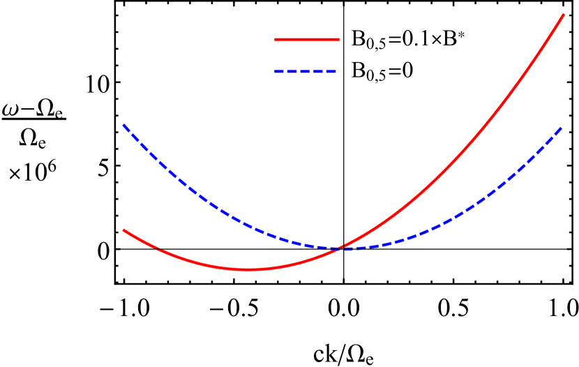
(a) $T=0$, $\mu_{5}=0$, $\mu=\sqrt{3\pi/(4\alpha)}\hbar\Omega_{e}$

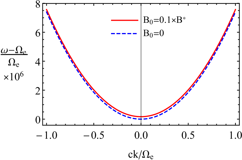
(b) $T=0$, $\mu_{5}=0$, $\mu=\sqrt{3\pi/(4\alpha)}\hbar\Omega_{e}$

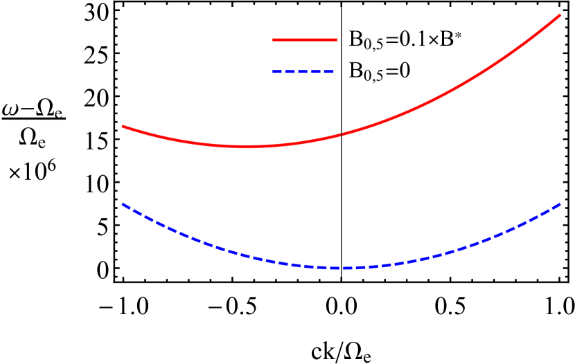
(c) $T=3\sqrt{1/(4\pi\alpha)}\hbar\Omega_{e}$, $\mu_{5}=0$, $\mu=0$

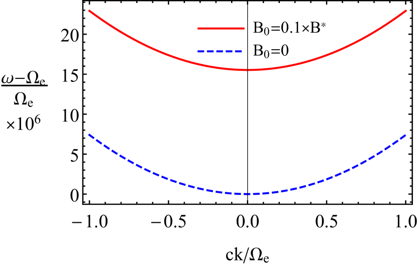
(d) $T=3\sqrt{1/(4\pi\alpha)}\hbar\Omega_{e}$, $\mu_{5}=0$, $\mu=0$

Figure 1: Left figures: The dispersion relation for the longitudinal mode propagating along the direction of background magnetic and pseudomagnetic fields with the wave vector $\mathbf{k}=k\hat{\mathbf{z}}$ at $B_{0,5}=0.1B^{*}$ (red solid line) and $B_{0,5}=0$ (blue dashed line). Right figures: The same dependence at $B_{0}=0.1B^{*}$ (red solid line) and $B_{0}=0$ (blue dashed line).

As we see from the left panel in Fig. 1, the dispersion relations for the CPMW have minima at nonzero values of the wave vectors. Their approximate locations are determined by $ck/\Omega_{e}\approx-5v_{F}\alpha eB_{0,5}/(3\pi\hbar\Omega_{e}^{2})$. We checked that interchanging the electric and chiral chemical potentials does not affect the properties of the CPMW.

Although the results in Fig. 1 show that the dispersion relations of the CMW and CPMW are indeed modified by the quadratic corrections in magnetic and pseudomagnetic fields, the corresponding effect is weak at small temperatures. The correction to the plasma gap is much larger at $T=3\sqrt{1/(4\pi\alpha)}\hbar\Omega_{e}$, $\mu_{5}=0$, and $\mu=0$, albeit it is still about five orders of magnitude smaller that the Langmuir frequency.

As we emphasized in Refs. Gorbar:2016ygi ; Gorbar:2016sey , the CMW and CPMW are chiral (pseudo)magnetic plasmons. Their chiral nature is evident from the fact that both electric $J_{z}$ and chiral $J_{z}^{5}$ current densities are oscillating in these waves. This can be seen from the explicit expressions for $J_{z}$ and $J_{z}^{5}$, given by Eqs. (100) and (101) in Appendix B, respectively. Leaving aside the technical details, we would like to emphasize only that the chiral current density oscillates in space and time, i.e., $J_{z}^{5}\propto E_{z}\sin{(\omega t-\mathbf{k}\cdot\mathbf{r})}$, which is similar to the electric current density, i.e., $J_{z}\propto E_{z}\sin{(\omega t-\mathbf{k}\cdot\mathbf{r})}$. Note, however, that the amplitudes of the currents are different and depend on the chiral chemical potential and the pseudomagnetic field.

IV Summary

By making use of the second-order corrections in (pseudo)electromagnetic fields to the quasiparticle energy, as well as the first-order corrections to the Berry curvature, we derived a consistent chiral kinetic theory valid to the second order in the electromagnetic and pseudoelectromagnetic fields for the simplest model of relativistic matter with two Weyl fermions. Such an extended theory allows one to study reliably various effects nonlinear in electromagnetic fields and is one of the main results of this paper.

While the semiclassical equations of motion preserve their form, the Berry curvature, as well as the quasiparticle dispersion relation receive nontrivial field-dependent corrections. However, we found that, even with the nontrivial corrections included, the Berry curvature $\mathbf{\Omega}_{\lambda}$ still defines a monopole-type vector field in the momentum space which corresponds to a unit of topological charge. Therefore, the chiral anomaly relation retains its canonical form in the second-order formulation of the chiral kinetic theory.

In order to illustrate the second-order consistent chiral kinetic theory, we analyzed the spectrum of longitudinal collective modes propagating along the direction of background magnetic and pseudomagnetic fields. We showed that, in the presence of a pseudomagnetic field, there is a different type of collective excitation similar to the chiral magnetic wave, which we call the chiral pseudomagnetic wave. The effects of dynamical electromagnetism play an important role and transform the chiral magnetic and chiral pseudomagnetic waves into plasmons with special properties. The latter manifest themselves in the oscillations of the chiral current density, which are absent in the case of ordinary electromagnetic plasmons.

We found that the plasmon gaps receive corrections quadratic in magnetic and pseudomagnetic fields, which cannot be reliably obtained within the conventional first-order chiral kinetic theory. Note, however, that these corrections are estimated to be rather weak compared to the effects of dynamical electromagnetism. In addition, the coefficients in front of odd powers of the wave vector in the dispersion relation of the chiral pseudomagnetic wave are nonzero and proportional to the background pseudomagnetic field. The coefficients in front of even powers depend on the square of both magnetic and pseudomagnetic fields. Nevertheless, the leading contributions to these coefficients are due to the effects of dynamical electromagnetism. It would be interesting to investigate how these conclusions about the CMW and CPMW change in the case of strong background magnetic and/or pseudomagnetic fields, and whether the effects of dynamical electromagnetism could be negligible. The corresponding problem requires a framework that goes beyond the expansion in powers of $\mathbf{B}_{0}$ and $\mathbf{B}_{0,5}$ and, therefore, will be considered elsewhere.

Appendix A Corrections to the Berry curvature, the quasiparticle energy, and the velocity

In this Appendix, we present the details of the derivation for the corrections to the Berry curvature, the quasiparticle energy, and the velocity, which are needed in the formulation of the chiral kinetic theory valid to the second order in (pseudo)electromagnetic fields.

Let us start from the derivation of the leading-order correction to the Berry curvature. By making use of the formalism of Refs. Gao:2014 ; Gao:2015 , the corresponding correction has the following standard form:

$$\mathbf{\Omega}_{\lambda}^{(1)}=(\bm{\nabla}_{\mathbf{p}}\times\mathbf{a}^{\prime}_{\lambda}),$$ (58)

where $\mathbf{a}^{\prime}_{\lambda}$ is a chirality ($\lambda=\pm$) and band-dependent ($\eta=\pm$) correction to the Berry connection or positional shift. This correction is given by

$$\mathbf{a}^{\prime}_{\lambda}=\sum_{\xi\neq\eta}\left\{\frac{G_{\eta,\xi}\mathbf{A}_{\xi,\eta}}{\epsilon^{(0)}_{\eta}-\epsilon^{(0)}_{\xi}}+\frac{e}{4c}\partial_{\mathbf{p}_{j}}\left([\mathbf{B}_{\lambda}\times\mathbf{A}_{\eta,\xi}]_{j}\mathbf{A}_{\xi,\eta}\right)\right\}+\frac{e\hbar^{2}}{v_{F}}\sum_{\xi\neq\eta}\frac{\mathbf{V}_{\eta\xi}(\mathbf{V}_{\xi\eta}\cdot\mathbf{E}_{\lambda})}{(\epsilon^{(0)}_{\eta}-\epsilon^{(0)}_{\xi})^{3}}+h.c.$$ (59)

Here, we used the interband matrix element associated with the magnetic dipole moment,

$$G_{\xi,\eta}=-\frac{e}{2c}\left\{\sum_{\gamma\neq\eta}\left(\mathbf{B}_{\lambda}\cdot[\mathbf{V}_{\xi,\gamma}\times\mathbf{A}_{\gamma,\eta}]\right)+\left(\mathbf{B}_{\lambda}\cdot[\mathbf{V}_{\eta,\eta}\times\mathbf{A}_{\xi,\eta}]\right)\right\},$$ (60)

which is defined in terms of the matrix elements of the velocity operator $\mathbf{V}=\lambda v_{F}\bm{\sigma}$ and the interband Berry connection, i.e.,

$$\mathbf{V}_{\xi,\eta} = \psi_{\xi}^{{\dagger}}\mathbf{V}\psi_{\eta},$$ (61)

$$\mathbf{A}_{\xi,\eta} = -i\hbar\psi_{\xi}^{{\dagger}}\bm{\partial}_{\mathbf{p}}\psi_{\eta},$$ (62)

respectively. Now, by making use of the normalized wave functions $\psi_{\eta}$ of the Weyl Hamiltonian (1)

$$\psi_{\eta} = \sqrt{\frac{p+\eta\lambda p_{z}}{2p}}\left(\begin{array}[]{c}1\\ \frac{p_{x}+ip_{y}}{p_{z}+\eta\lambda p}\\ \end{array}\right),$$ (65)

we obtain the following explicit expressions for the correction to the Berry connection:

$$\mathbf{a}^{\prime}_{\lambda}=\frac{e\hbar^{2}}{8p^{3}}\left\{\frac{1}{c}[\mathbf{B}_{\lambda}\times\hat{\mathbf{p}}]+\frac{2\eta}{v_{F}}\left[\mathbf{E}_{\lambda}-\hat{\mathbf{p}}(\hat{\mathbf{p}}\cdot\mathbf{E}_{\lambda})\right]\right\},$$ (66)

where $\hat{\mathbf{p}}=\mathbf{p}/p$. Finally, by making use of Eq. (58), we obtain the leading-order correction to the Berry curvature, i.e.,

$$\mathbf{\Omega}_{\lambda}^{(1)}=\frac{e\hbar^{2}}{4p^{4}}\left\{\frac{2}{c}\hat{\mathbf{p}}(\hat{\mathbf{p}}\cdot\mathbf{B}_{\lambda})-\frac{1}{c}\mathbf{B}_{\lambda}+\frac{2\eta}{v_{F}}[\mathbf{E}_{\lambda}\times\hat{\mathbf{p}}]\right\}.$$ (67)

It remains to determine the quasiparticle dispersion relation to the second order in (pseudo)electromagnetic fields for the model at hand. The corresponding general expression reads as follows Gao:2015 :

$$\epsilon_{\mathbf{p}}=\epsilon^{(0)}_{\eta}-\frac{e}{c}(\mathbf{B}_{\lambda}\cdot\mathbf{m})+\frac{e^{2}}{4c^{2}}(\mathbf{B}_{\lambda}\cdot\mathbf{\Omega}_{\lambda}^{(0)})(\mathbf{B}_{\lambda}\cdot\mathbf{m})-\frac{e}{c}(\mathbf{B}_{\lambda}\cdot[\mathbf{a}_{\lambda}^{\prime}\times\mathbf{V}_{\eta,\eta}])+(\bm{\nabla}_{\mathbf{p}}\cdot\mathbf{P}_{E})+\sum_{\xi\neq\eta}\frac{G_{\eta\xi}G_{\xi,\eta}}{\epsilon^{(0)}_{\eta}-\epsilon^{(0)}_{\xi}},$$ (68)

where the orbital magnetic moment equals

$$\mathbf{m}=\frac{1}{2}\mathrm{Im}\left[(\bm{\partial}_{\mathbf{p}}\psi_{\eta})^{{\dagger}}\times\left(\epsilon^{(0)}_{\eta}-\hat{H}\right)(\bm{\partial}_{\mathbf{p}}\psi_{\eta})\right]=\epsilon^{(0)}_{\eta}\mathbf{\Omega}_{\lambda}^{(0)}$$ (69)

and

$$\mathbf{P}_{E}=\frac{e^{2}\hbar^{2}}{4c^{2}}\left\{([\mathbf{B}_{\lambda}\times\bm{D}]\psi_{\eta})^{{\dagger}}(\mathbf{V}+\mathbf{V}_{\eta,\eta})([\mathbf{B}_{\lambda}\times\bm{D}]\psi_{\eta})+h.c.\right\}$$ (70)

is the energy polarization density. Here, $\mathbf{D}=\hbar\bm{\partial}_{\mathbf{p}}-i\mathbf{A}_{\eta,\eta}$ is the gauge covariant derivative. After lengthy but straightforward calculations, we found that $\mathbf{P}_{E}=\mathbf{0}$ for the Weyl Hamiltonian (1). Moreover, one can check that all off-diagonal interband mixing terms vanish, i.e., $G_{-\eta,\eta}=0$. The fourth term in Eq. (68) reads as

$$-\frac{e}{c}\left(\mathbf{B}_{\lambda}\cdot[\mathbf{a}_{\lambda}^{\prime}\times\mathbf{V}_{\eta,\eta}]\right) = \frac{e^{2}\hbar^{2}}{4cp^{4}}\left\{\frac{\eta v_{F}}{2pc}\left[B_{\lambda}^{2}p^{2}-(\mathbf{B}_{\lambda}\cdot\mathbf{p})^{2}\right]-\left(\mathbf{B}_{\lambda}\cdot[\mathbf{E}_{\lambda}\times\mathbf{p}]\right)\right\}.$$ (71)

Thus, one finds that the quasiparticle dispersion relation (68) to the second order in (pseudo)electromagnetic fields equals

$$\epsilon_{\mathbf{p}}\equiv\epsilon^{(0)}_{\eta}+\epsilon_{\eta}^{(1)}+\epsilon_{\eta}^{(2)}=\eta v_{F}p-\lambda\frac{e\hbar v_{F}}{2cp}(\mathbf{B}_{\lambda}\cdot\hat{\mathbf{p}})+\frac{e^{2}\hbar^{2}}{4cp^{3}}\left\{\frac{\eta v_{F}}{4c}\left[2B_{\lambda}^{2}-(\mathbf{B}_{\lambda}\cdot\hat{\mathbf{p}})^{2}\right]-(\mathbf{B}_{\lambda}\cdot[\mathbf{E}_{\lambda}\times\hat{\mathbf{p}}])\right\},$$ (72)

where

$$\epsilon_{\eta}^{(0)} = \eta v_{F}p,$$ (73)

$$\epsilon_{\eta}^{(1)} = -\eta\frac{ev_{F}p}{c}(\mathbf{B}_{\lambda}\cdot\mathbf{\Omega}_{\lambda}^{(0)})=-\lambda\frac{e\hbar v_{F}}{2cp}(\mathbf{B}_{\lambda}\cdot\hat{\mathbf{p}}),$$ (74)

$$\epsilon_{\eta}^{(2)} = \eta\frac{e^{2}v_{F}p}{4c^{2}}(\mathbf{B}_{\lambda}\cdot\mathbf{\Omega}_{\lambda}^{(0)})^{2}+\frac{e^{2}\hbar^{2}}{4cp^{4}}\left\{\frac{\eta v_{F}}{2pc}\left[B_{\lambda}^{2}p^{2}-(\mathbf{B}_{\lambda}\cdot\mathbf{p})^{2}\right]-\left(\mathbf{B}_{\lambda}\cdot[\mathbf{E}_{\lambda}\times\mathbf{p}]\right)\right\}$$ (75)

$$= \frac{e^{2}\hbar^{2}}{4cp^{3}}\left\{\frac{\eta v_{F}}{4c}\left[2B_{\lambda}^{2}-(\mathbf{B}_{\lambda}\cdot\hat{\mathbf{p}})^{2}\right]-(\mathbf{B}_{\lambda}\cdot[\mathbf{E}_{\lambda}\times\hat{\mathbf{p}}])\right\}.$$

The corresponding quasiparticle velocity is given by

$$\mathbf{v}=\frac{\partial\epsilon_{\mathbf{p}}}{\partial\mathbf{p}}=\mathbf{v}^{(0)}+\mathbf{v}^{(1)}+\mathbf{v}^{(2)},$$ (76)

where

$$\mathbf{v}^{(0)} = \eta v_{F}\hat{\mathbf{p}},$$ (77)

$$\mathbf{v}^{(1)} = \lambda\frac{ev_{F}\hbar}{c}\hat{\mathbf{p}}\frac{(\hat{\mathbf{p}}\cdot\mathbf{B}_{\lambda})}{p^{2}}-\lambda\frac{ev_{F}\hbar}{c}\frac{\mathbf{B}_{\lambda}}{2p^{2}},$$ (78)

$$\mathbf{v}^{(2)} = \frac{5\eta e^{2}v_{F}\hbar^{2}\hat{\mathbf{p}}(\mathbf{B}_{\lambda}\cdot\hat{\mathbf{p}})^{2}}{16c^{2}p^{4}}-\frac{\eta e^{2}v_{F}\hbar^{2}\mathbf{B}_{\lambda}(\mathbf{B}_{\lambda}\cdot\hat{\mathbf{p}})}{8c^{2}p^{4}}-\frac{3\eta e^{2}\hbar^{2}v_{F}}{8c^{2}p^{4}}\hat{\mathbf{p}}B_{\lambda}^{2}+\frac{e^{2}\hbar^{2}}{4cp^{4}}(\mathbf{E}_{\lambda}\times\mathbf{B}_{\lambda})+\frac{e^{2}\hbar^{2}}{cp^{4}}\hat{\mathbf{p}}(\mathbf{B}_{\lambda}\cdot[\mathbf{E}_{\lambda}\times\hat{\mathbf{p}}]).$$

Appendix B Polarization vector and currents

In this Appendix, we provide the details of the calculation of the polarization vector (32) and present an explicit form of the electric and chiral currents for the chiral magnetic and pseudomagnetic waves. Using Eqs. (33) through (35) from the main text and integrating over polar and azimuthal angles, one can show that $\mathbf{P}^{\prime(0)}=\mathbf{P}_{M}^{\prime(0)}=\mathbf{P}_{M}^{\prime(1)}=\mathbf{0}$ and $P_{x}^{\prime(1)}=P_{y}^{\prime(1)}=0$. Moreover, for $\mathbf{b}\parallel\hat{\mathbf{z}}$, the topological part of the polarization vector (33) is also absent, i.e., $\mathbf{P}_{T}=\mathbf{0}$. However, the component of the polarization vector along the direction of (pseudo)magnetic field $\hat{\mathbf{z}}$ is nonzero and equals

$$P_{z}^{\prime(1)}=\left(\chi_{0}^{33}+\chi_{1}^{33}+\chi_{2}^{33}\right)E_{z}^{\prime}.$$ (80)

Components of the susceptibility tensor $\chi^{33}$ equal

$$\chi_{0}^{33} = -\sum_{\lambda=\pm}\sum_{\eta=\pm}\eta\int dp\,p^{2}\frac{e^{2}}{2\pi^{2}\hbar^{3}k^{2}}\left[1-\eta\frac{\omega}{2v_{F}k}\ln{\left(\frac{\eta\omega+v_{F}k}{\eta\omega-v_{F}k}\right)}\right]f_{1},$$ (81)

$$\chi_{1}^{33} = -\sum_{\lambda=\pm}\sum_{\eta=\pm}\eta\int dp\frac{e^{3}\eta\lambda B_{0,\lambda}}{24\pi^{2}c\hbar^{2}v_{F}^{2}k^{4}(\omega^{2}-v_{F}^{2}k^{2})}\Big{\{}2\eta v_{F}k\left[-v_{F}^{4}k^{4}(2f_{1}-f_{2})+2\omega^{2}v_{F}^{2}k^{2}(f_{1}+f_{2})-3\omega^{4}(f_{1}+f_{2})\right]$$ (82)

$$+ 3\omega^{3}(\omega^{2}-v_{F}^{2}k^{2})(f_{1}+f_{2})\ln{\left(\frac{\eta\omega+v_{F}k}{\eta\omega-v_{F}k}\right)}\Big{\}},$$

$$\chi_{2}^{33} = \sum_{\lambda=\pm}\sum_{\eta=\pm}\eta\int\frac{dp}{p^{2}}\frac{\eta e^{4}B_{0,\lambda}^{2}}{192\pi^{2}c^{2}\hbar v_{F}^{3}k^{5}(\omega^{2}-v_{F}^{2}k^{2})^{2}}\Bigg{\{}2\eta v_{F}k\Big{[}v_{F}^{6}k^{6}(4f_{1}-f_{2}-2f_{3})-\omega^{2}v_{F}^{4}k^{4}(98f_{1}+7f_{2}+2f_{3})$$ (83)

$$+ \omega^{4}v_{F}^{2}k^{2}(229f_{1}+29f_{2}+10f_{3})-3\omega^{6}(41f_{1}+7f_{2}+2f_{3})\Big{]}$$

$$- 3\omega(\omega^{2}-v_{F}^{2}k^{2})^{2}\left[2v_{F}^{2}k^{2}(4f_{1}-f_{2})-\omega^{2}(41f_{1}+7f_{2}+2f_{3})\right]\ln{\left(\frac{\eta\omega+v_{F}k}{\eta\omega-v_{F}k}\right)}\Bigg{\}},$$

where

$$f_{1} = \frac{\partial f^{(0)}_{\lambda}}{\partial\epsilon_{\mathbf{p}}},$$ (84)

$$f_{2} = \eta v_{F}p\frac{\partial^{2}f^{(0)}_{\lambda}}{\partial\epsilon_{\mathbf{p}}^{2}},$$ (85)

$$f_{3} = (v_{F}p)^{2}\frac{\partial^{3}f^{(0)}_{\lambda}}{\partial\epsilon_{\mathbf{p}}^{3}},$$ (86)

and we used the following integrals:

$$\int dp\,p^{2}\frac{\partial f^{(0)}_{\lambda}}{\partial\epsilon_{\mathbf{p}}} = \eta\frac{2T^{2}}{v_{F}^{3}}\mbox{Li}_{2}\left(-e^{\eta\mu_{\lambda}/T}\right),$$ (87)

$$\int dp\,\frac{\partial f^{(0)}_{\lambda}}{\partial\epsilon_{\mathbf{p}}} = -\frac{\eta}{v_{F}}\frac{1}{1+e^{-\eta\mu_{\lambda}/T}},$$ (88)

$$\int dp\,p\frac{\partial^{2}f^{(0)}_{\lambda}}{\partial\epsilon_{\mathbf{p}}^{2}} = \frac{1}{v_{F}^{2}}\frac{1}{1+e^{-\eta\mu_{\lambda}/T}},$$ (89)

$$\int\frac{dp}{p^{2}}\frac{\partial f^{(0)}_{\lambda}}{\partial\epsilon_{\mathbf{p}}} = \eta v_{F}\Bigg{\{}-\frac{1}{\eta v_{F}p}\frac{\partial f^{(0)}_{\lambda}}{\partial\epsilon_{\mathbf{p}}}\Big{|}^{\infty}_{\Lambda_{\rm IR}}+\int_{\Lambda_{\rm IR}}^{\infty}\frac{dp}{p}\frac{\partial^{2}f^{(0)}_{\lambda}}{\partial\epsilon_{\mathbf{p}}^{2}}\Bigg{\}}=-\frac{\eta}{4T\Lambda_{\rm IR}\cosh^{2}{\left(\frac{\mu_{\lambda}}{2T}\right)}}+\eta v_{F}\int_{\Lambda_{\rm IR}}^{\infty}\frac{dp}{p}\frac{\partial^{2}f^{(0)}_{\lambda}}{\partial\epsilon_{\mathbf{p}}^{2}},$$ (90)

$$\int\frac{dp}{p}\frac{\partial^{2}f^{(0)}_{\lambda}}{\partial\epsilon_{\mathbf{p}}^{2}} = \int_{\Lambda_{\rm IR}}^{\infty}\frac{dp}{p}\frac{\partial^{2}f^{(0)}_{\lambda}}{\partial\epsilon_{\mathbf{p}}^{2}},$$ (91)

$$\int dp\frac{\partial^{3}f^{(0)}_{\lambda}}{\partial\epsilon_{\mathbf{p}}^{3}} = \frac{\eta}{4v_{F}T^{2}}\frac{\tanh{\left(\frac{\eta\mu_{\lambda}}{2T}\right)}}{\cosh^{2}{\left(\frac{\mu_{\lambda}}{2T}\right)}}.$$ (92)

Here, the equilibrium distribution function was expanded as

$$f_{\lambda}^{\rm(eq)}\simeq f_{\lambda}^{(0)}+\left(\epsilon^{(1)}_{\eta}+\epsilon^{(2)}_{\eta}\right)\frac{\partial f^{(0)}_{\lambda}}{\partial\epsilon_{\mathbf{p}}}+\frac{\left(\epsilon^{(1)}_{\eta}\right)^{2}}{2}\frac{\partial^{2}f^{(0)}_{\lambda}}{\partial\epsilon_{\mathbf{p}}^{2}}+O(B_{0,\lambda}^{3}),$$ (93)

where $f_{\lambda}^{(0)}$ is given by Eq. (23) with $\epsilon_{\mathbf{p}}=\epsilon^{(0)}_{\eta}$. While the quasiparticle energy without electromagnetic fields $\epsilon^{(0)}_{\eta}$ is given by Eq. (73), the field-dependent corrections $\epsilon^{(1)}_{\eta}$ and $\epsilon^{(2)}_{\eta}$ are given by Eqs. (74) and (75), respectively. Next, we introduced an infrared cutoff $\Lambda_{\rm IR}=C\sqrt{\hbar|eB_{0,\lambda}|/c}$ with a numerical constant $C$ of order unity. Such a cutoff has a transparent physical meaning: It separates the phase space of large momenta, where the semiclassical description is valid, from the infrared region $p\lesssim\Lambda_{\rm IR}$, where such a description fails (for details, see also Ref. Stephanov:2012ki ). In our numerical calculations, we will use $C=1$. After adding the contribution of antiparticles, one can set $\Lambda_{\rm IR}$ to zero in the last term of the fourth integral and in the fifth integral because the corresponding integrals are no longer divergent in the infrared region and can be expressed in terms of the derivative of the function

$$F\left(\nu_{\lambda}\right)\equiv-T\sum_{\eta=\pm}\int\frac{dp}{p}\frac{\partial f^{(0)}_{\lambda}}{\partial\epsilon_{\mathbf{p}}}$$ (94)

with respect to $\nu_{\lambda}\equiv\mu_{\lambda}/T$, i.e.,

$$\frac{1}{T^{2}}\frac{\partial F\left(\nu_{\lambda}\right)}{\partial\nu_{\lambda}}=\sum_{\eta=\pm}\eta\int_{0}^{\infty}\frac{dp}{p}\frac{\partial^{2}f^{(0)}_{\lambda}}{\partial\epsilon_{\mathbf{p}}^{2}}.$$ (95)

High- and low-temperature asymptotes of $F(\nu_{\lambda})$ equal $F\left(\nu_{\lambda}\right)\simeq 7\zeta(3)\nu_{\lambda}/(2\pi^{2})\approx 0.426\nu_{\lambda}$ for $T\to\infty$ and $F\left(\nu_{\lambda}\right)\simeq\nu_{\lambda}^{-1}$ for $T\to 0$, respectively. The function $F\left(\nu_{\lambda}\right)$ could be well approximated by the Padé approximant of order [5/6], i.e.,

$$F\left(\nu_{\lambda}\right)\simeq\frac{7\zeta(3)}{2\pi^{2}}\frac{\nu_{\lambda}+0.03533\nu_{\lambda}^{3}+0.0007432\nu_{\lambda}^{5}}{1+0.2290\nu_{\lambda}^{2}+0.01567\nu_{\lambda}^{4}+0.0003098\nu_{\lambda}^{6}}.$$ (96)

Using Eqs. (87)-(92), we obtain

$${\chi_{0}^{33}} = -\sum_{\eta=\pm}\sum_{\lambda=\pm}\frac{e^{2}}{2\pi^{2}\hbar^{3}k^{2}}\left[1-\eta\frac{\omega}{2v_{F}k}\ln{\left(\frac{\eta\omega+v_{F}k}{\eta\omega-v_{F}k}\right)}\right]\frac{T^{2}}{v_{F}^{3}}\mbox{Li}_{2}\left(-e^{\eta\mu_{\lambda}/T}\right),$$ (97)

$${\chi_{1}^{33}} = -\sum_{\eta=\pm}\sum_{\lambda=\pm}\frac{e^{3}\lambda B_{0,\lambda}v_{F}^{2}k}{4\pi^{2}c\hbar^{2}\omega(\omega^{2}-v_{F}^{2}k^{2})}\frac{1}{1+e^{-\eta\mu_{\lambda}}},$$ (98)

$${\chi_{2}^{33}} = -\sum_{\eta=\pm}\sum_{\lambda=\pm}\frac{1}{4T\Lambda_{\rm IR}\cosh^{2}{\left(\frac{\mu_{\lambda}}{2T}\right)}}\frac{e^{4}B_{0,\lambda}^{2}}{192c^{2}\pi^{2}\hbar v_{F}^{3}k^{5}(\omega^{2}-v_{F}^{2}k^{2})^{2}}\Bigg{[}2v_{F}k\left(4v_{F}^{6}k^{6}-98\omega^{2}v_{F}^{4}k^{4}+229\omega^{4}v_{F}^{2}k^{2}-123\omega^{6}\right)$$ (99)

$$+ 3\eta\omega\left(41\omega^{2}-8v_{F}^{2}k^{2}\right)(\omega^{2}-v_{F}^{2}k^{2})^{2}\ln{\left(\frac{\eta\omega+v_{F}k}{\eta\omega-v_{F}k}\right)}\Bigg{]}$$

$$+ \sum_{\eta=\pm}\sum_{\lambda=\pm}\frac{1}{T}\frac{\partial F\left(\frac{\mu_{\lambda}}{T}\right)}{\partial\mu_{\lambda}}\frac{e^{4}B_{0,\lambda}^{2}}{192c^{2}\pi^{2}\hbar v_{F}^{2}k^{5}(\omega^{2}-v_{F}^{2}k^{2})^{2}}\Bigg{[}6v_{F}k\left(v_{F}^{6}k^{6}-35\omega^{2}v_{F}^{4}k^{4}+86\omega^{4}v_{F}^{2}k^{2}-48\omega^{6}\right)$$

$$+ 6\eta\omega\left(24\omega^{2}-3v_{F}^{2}k^{2}\right)(\omega^{2}-v_{F}^{2}k^{2})\ln{\left(\frac{\eta\omega+v_{F}k}{\eta\omega-v_{F}k}\right)}\Bigg{]}$$

$$- \sum_{\eta=\pm}\sum_{\lambda=\pm}\frac{1}{4v_{F}T^{2}}\frac{\tanh{\left(\frac{\eta\mu_{\lambda}}{2T}\right)}}{\cosh^{2}{\left(\frac{\mu_{\lambda}}{2T}\right)}}\frac{e^{4}B_{0,\lambda}^{2}}{192c^{2}\pi^{2}\hbar v_{F}k^{5}}\Bigg{[}4v_{F}k(3\omega^{2}+v_{F}^{2}k^{2})-6\eta\omega^{3}\ln{\left(\frac{\eta\omega+v_{F}k}{\eta\omega-v_{F}k}\right)}\Bigg{]}.$$

Further, let us present explicit expressions for the nonzero components of the electric $J_{z}$ and chiral $J_{z}^{5}$ current densities, i.e.,

$$J_{z} = E_{z}\sin{(\omega t-\mathbf{k}\cdot\mathbf{r})}\frac{3\omega n_{0}^{2}\Omega_{e}^{2}}{4\pi v_{F}^{2}k^{2}}\left[1-\frac{\omega}{2v_{F}k}\ln{\left(\frac{\omega+v_{F}k}{\omega-v_{F}k}\right)}\right]$$ (100)

$$+ E_{z}\sin{(\omega t-\mathbf{k}\cdot\mathbf{r})}\frac{\alpha n_{0}^{2}e(\mathbf{B}_{0,5}\cdot\mathbf{k})v_{F}^{3}}{2\pi^{2}c\hbar(\omega^{2}-v_{F}^{2}k^{2})}$$

$$+ E_{z}\sin{(\omega t-\mathbf{k}\cdot\mathbf{r})}\sum_{\lambda=\pm}\frac{1}{T}F_{1}\left(\frac{\mu_{\lambda}}{T},B_{0,\lambda}\right)\frac{\alpha^{2}\hbar n_{0}^{4}B_{0,\lambda}^{2}\omega}{192c^{2}\pi^{2}v_{F}k^{5}(\omega^{2}-v_{F}^{2}k^{2})^{2}}\Bigg{[}2v_{F}k\left(4v_{F}^{6}k^{6}-98\omega^{2}v_{F}^{4}k^{4}+229v_{F}^{2}k^{2}\omega^{4}-123\omega^{6}\right)$$

$$+ 3\omega\left(41\omega^{2}-8v_{F}^{2}k^{2}\right)(\omega^{2}-v_{F}^{2}k^{2})^{2}\ln{\left(\frac{\omega+v_{F}k}{\omega-v_{F}k}\right)}\Bigg{]}$$

$$- E_{z}\sin{(\omega t-\mathbf{k}\cdot\mathbf{r})}\sum_{\lambda=\pm}\frac{1}{T^{2}}F_{2}\left(\frac{\mu_{\lambda}}{T}\right)\frac{\alpha^{2}\hbar n_{0}^{4}B_{0,\lambda}^{2}\omega}{192c^{2}\pi^{2}k^{5}(\omega^{2}-v_{F}^{2}k^{2})^{2}}\Bigg{[}6v_{F}k\left(v_{F}^{6}k^{6}-35\omega^{2}v_{F}^{4}k^{4}+86\omega^{4}v_{F}^{2}k^{2}-48\omega^{6}\right)$$

$$+ 6\omega\left(24\omega^{2}-3v_{F}^{2}k^{2}\right)(\omega^{2}-v_{F}^{2}k^{2})^{2}\ln{\left(\frac{\omega+v_{F}k}{\omega-v_{F}k}\right)}\Bigg{]}$$

and

$$J_{z}^{5} = E_{z}\sin{(\omega t-\mathbf{k}\cdot\mathbf{r})}\frac{2\alpha n_{0}^{2}\omega\mu\mu_{5}}{\pi^{2}\hbar^{2}v_{F}^{2}k^{2}}\left[1-\frac{\omega}{2v_{F}k}\ln{\left(\frac{\omega+v_{F}k}{\omega-v_{F}k}\right)}\right]$$ (101)

$$+ E_{z}\sin{(\omega t-\mathbf{k}\cdot\mathbf{r})}\frac{\alpha n_{0}^{2}e(\mathbf{B}_{0}\cdot\mathbf{k})v_{F}^{3}}{2\pi^{2}c\hbar(\omega^{2}-v_{F}^{2}k^{2})}$$

$$+ E_{z}\sin{(\omega t-\mathbf{k}\cdot\mathbf{r})}\sum_{\lambda=\pm}\frac{\lambda}{T}F_{1}\left(\frac{\mu_{\lambda}}{T},B_{0,\lambda}\right)\frac{\alpha^{2}\hbar n_{0}^{4}B_{0,\lambda}^{2}\omega}{192c^{2}\pi^{2}v_{F}k^{5}(\omega^{2}-v_{F}^{2}k^{2})^{2}}\Bigg{[}2v_{F}k\left(4v_{F}^{6}k^{6}-98\omega^{2}v_{F}^{4}k^{4}+229v_{F}^{2}k^{2}\omega^{4}-123\omega^{6}\right)$$

$$+ 3\omega\left(41\omega^{2}-8v_{F}^{2}k^{2}\right)(\omega^{2}-v_{F}^{2}k^{2})^{2}\ln{\left(\frac{\omega+v_{F}k}{\omega-v_{F}k}\right)}\Bigg{]}$$

$$- E_{z}\sin{(\omega t-\mathbf{k}\cdot\mathbf{r})}\sum_{\lambda=\pm}\frac{\lambda}{T^{2}}F_{2}\left(\frac{\mu_{\lambda}}{T}\right)\frac{\alpha^{2}\hbar n_{0}^{4}B_{0,\lambda}^{2}\omega}{192c^{2}\pi^{2}k^{5}(\omega^{2}-v_{F}^{2}k^{2})^{2}}\Bigg{[}6v_{F}k\left(v_{F}^{6}k^{6}-35\omega^{2}v_{F}^{4}k^{4}+86\omega^{4}v_{F}^{2}k^{2}-48\omega^{6}\right)$$

$$+ 6\omega\left(24\omega^{2}-3v_{F}^{2}k^{2}\right)(\omega^{2}-v_{F}^{2}k^{2})^{2}\ln{\left(\frac{\omega+v_{F}k}{\omega-v_{F}k}\right)}\Bigg{]},$$

respectively. Here, functions $F_{1}(x,y)$ and $F_{2}(x)$ are given by Eqs. (55) and (56) in the main text. As one can see from the above expressions, both electric and chiral current densities are oscillating in the chiral magnetic and pseudomagnetic waves, albeit with different amplitudes.

References

- (1) E. M. Lifshitz and L. P. Pitaevskii, Physical Kinetics (Pergamon, New York, 1981).
- (2) N. A. Krall and A. W. Trivelpiece, Principles of Plasma Physics (Mc-Graw Hill, New York, 1973).
- (3) J. P. Vallee, New Astron. Rev. 55, 91 (2011).
- (4) R. Durrer and A. Neronov, Astron. Astrophys. Rev. 21, 62 (2013).
- (5) D. E. Kharzeev, L. D. McLerran, and H. J. Warringa, Nucl. Phys. A 803, 227 (2008).
- (6) D. E. Kharzeev, J. Liao, S. A. Voloshin, and G. Wang, Prog. Part. Nucl. Phys. 88, 1 (2016).
- (7) C. Kouveliotou, T. Strohmayer, K. Hurley, J. van Paradijs, M. H. Finger, S. Dieters, P. Woods, C. Thompson, and R. S. Duncan, Astrophys. J. 510, L115 (1999).
- (8) Z. Wang, Y. Sun, X. Q. Chen, C. Franchini, G. Xu, H. Weng, X. Dai, and Z. Fang, Phys. Rev. B 85, 195320 (2012).
- (9) Z. Wang, H. Weng, Q. Wu, X. Dai, and Z. Fang, Phys. Rev. B 88, 125427 (2013).
- (10) H. Weng, X. Dai, and Z. Fang, Phys. Rev. X 4, 011002 (2014).
- (11) S. Borisenko, Q. Gibson, D. Evtushinsky, V. Zabolotnyy, B. Buchner, and R. J. Cava, Phys. Rev. Lett. 113, 027603 (2014).
- (12) M. Neupane, S.-Y. Xu, R. Sankar, N. Alidoust, G. Bian, C. Liu, I. Belopolski, T.-R. Chang, H.-T. Jeng, H. Lin, A. Bansil, F. Chou, and M. Z. Hasan, Nat. Commun. 5, 3786 (2014).
- (13) Z. K. Liu, B. Zhou, Y. Zhang, Z. J. Wang, H. M. Weng, D. Prabhakaran, S.-K. Mo, Z. X. Shen, Z. Fang, X. Dai, Z. Hussain, and Y. L. Chen, Science 343, 864 (2014).
- (14) J. Xiong, S. K. Kushwaha, T. Liang, J. W. Krizan, M. Hirschberger, W. Wang, R. J. Cava, N. P. Ong, Science 350, 413 (2015).
- (15) C.-Z. Li, L.-X. Wang, H. Liu, J. Wang, Z.-M. Liao, and D.-P. Yu, Nat. Commun. 6, 10137 (2015).
- (16) H. Li, H. He, H.-Z. Lu, H. Zhang, H. Liu, R. Ma, Z. Fan, S.-Q. Shen, and J. Wang, Nat. Commun. 7, 10301 (2016).
- (17) Q. Li, D. E. Kharzeev, C. Zhang, Y. Huang, I. Pletikosic, A. V. Fedorov, R. D. Zhong, J. A. Schneeloch, G. D. Gu, and T. Valla, Nat. Phys. 12, 550 (2016).
- (18) G. Zheng, J. Lu, X. Zhu, W. Ning, Y. Han, H. Zhang, J. Zhang, C. Xi, J. Yang, H. Du, K. Yang, Y. Zhang, and M. Tian, Phys. Rev. B 93, 115414 (2016).
- (19) X. Wan, A. M. Turner, A. Vishwanath, and S. Y. Savrasov, Phys. Rev. B 83, 205101 (2011).
- (20) H. M. Weng, C. Fang, Z. Fang, B. A. Bernevig, and X. Dai, Phys. Rev. X 5, 011029 (2015).
- (21) B. Q. Lv, H. M. Weng, B. B. Fu, X. P. Wang, H. Miao, J. Ma, P. Richard, X. C. Huang, L. X. Zhao, G. F. Chen, Z. Fang, X. Dai, T. Qian, and H. Ding, Phys. Rev. X 5, 031013 (2015).
- (22) X. Huang, L. Zhao, Y. Long, P. Wang, D. Chen, Z. Yang, H. Liang, M. Xue, H. Weng, Z. Fang, X. Dai, and G. Chen, Phys. Rev. X 5, 031023 (2015).
- (23) S.-Y. Xu, I. Belopolski, N. Alidoust, M. Neupane, G. Bian, C. Zhang, R. Sankar, G. Chang, Z. Yuan, C.-C. Lee, S.-M. Huang, H. Zheng, J. Ma, D. S. Sanchez, B. Wang, A. Bansil, F. Chou, P. P. Shibayev, H. Lin, S. Jia, and M. Z. Hasan, Science 349, 613 (2015).
- (24) S.-M. Huang, S.-Y. Xu, I. Belopolski, C.-C. Lee, G. Chang, B. Wang, N. Alidoust, G. Bian, M. Neupane, C. Zhang, S. Jia, A. Bansil, H. Lin, and M. Z. Hasan Nat. Commun. 6, 7373 (2015).
- (25) C.-L. Zhang, S.-Y. Xu, I. Belopolski, Z. Yuan, Z. Lin, B. Tong, G. Bian, N. Alidoust, C.-C. Lee, S.-M. Huang, T.-R. Chang, G. Chang, C.-H. Hsu, H.-T. Jeng, M. Neupane, D. S. Sanchez, H. Zheng, J. Wang, H. Lin, C. Zhang, H.-Z. Lu, S.-Q. Shen, T. Neupert, M. Z. Hasan, and S. Jia, Nat. Commun. 7, 10735 (2016).
- (26) S. Borisenko, D. Evtushinsky, Q. Gibson, A. Yaresko, T. Kim, M. N. Ali, B. Buechner, M. Hoesch, and R. J. Cava, arXiv:1507.04847.
- (27) I. Belopolski, S.-Y. Xu, Y. Ishida, X. Pan, P. Yu, D. S. Sanchez, M. Neupane, N. Alidoust, G. Chang, T.-R. Chang, Y. Wu, G. Bian, H. Zheng, S.-M. Huang, C.-C. Lee, D. Mou, L. Huang, Y. Song, B. Wang, G. Wang, Y.-W. Yeh, N. Yao, J. Rault, P. Lefevre, F. Bertran, H.-T. Jeng, T. Kondo, A. Kaminski, H. Lin, Z. Liu, F. Song, S. Shin, and M. Z. Hasan, arXiv:1512.09099.
- (28) S. L. Adler, Phys. Rev. 177, 2426 (1969); J. S. Bell and R. Jackiw, Nuovo Cimento A 60, 47 (1969).
- (29) D. T. Son and N. Yamamoto, Phys. Rev. Lett. 109, 181602 (2012); Phys. Rev. D 87, 085016 (2013).
- (30) M. A. Stephanov and Y. Yin, Phys. Rev. Lett. 109, 162001 (2012).
- (31) H. B. Nielsen and M. Ninomiya, Phys. Lett. B 130, 389 (1983).
- (32) D. T. Son and B. Z. Spivak, Phys. Rev. B 88, 104412 (2013).
- (33) V. Aji, Phys. Rev. B 85, 241101 (2012).
- (34) H.-J. Kim, K.-S. Kim, J. F. Wang, M. Sasaki, N. Satoh, A. Ohnishi, M. Kitaura, M. Yang, and L. Li, Phys. Rev. Lett. 111, 246603 (2013).
- (35) E. V. Gorbar, V. A. Miransky, and I. A. Shovkovy, Phys. Rev. B 89, 085126 (2014).
- (36) A. A. Burkov, Phys. Rev. B 91, 245157 (2015).
- (37) D. E. Kharzeev and H. U. Yee, Phys. Rev. D 83, 085007 (2011).
- (38) Y. Akamatsu and N. Yamamoto, Phys. Rev. Lett. 111, 052002 (2013).
- (39) M. Stephanov, H. U. Yee, and Y. Yin, Phys. Rev. D 91, 125014 (2015).
- (40) E. V. Gorbar, V. A. Miransky, I. A. Shovkovy, and P. O. Sukhachov, Phys. Rev. Lett. 118, 127601 (2017).
- (41) E. V. Gorbar, V. A. Miransky, I. A. Shovkovy, and P. O. Sukhachov, Phys. Rev. B 95, 115202 (2017).
- (42) M. A. Zubkov, Ann. Phys. 360, 655 (2015).
- (43) A. Cortijo, Y. Ferreiros, K. Landsteiner, and M. A. H. Vozmediano, Phys. Rev. Lett. 115, 177202 (2015).
- (44) D. I. Pikulin, A. Chen, and M. Franz, Phys. Rev. X 6, 041021 (2016).
- (45) A. Cortijo, D. Kharzeev, K. Landsteiner, and M. A. H. Vozmediano, Phys. Rev. B 94, 241405 (2016).
- (46) A. G. Grushin, J. W. F. Venderbos, A. Vishwanath, and R. Ilan, Phys. Rev. X 6, 041046 (2016).
- (47) T. Liu, D. I. Pikulin, and M. Franz, Phys. Rev. B 95, 041201 (2017).
- (48) H. B. Nielsen and M. Ninomiya, Nucl. Phys. B 185, 20 (1981); 195, 541 (1982).
- (49) F. M. D. Pellegrino, M. I. Katsnelson, and M. Polini, Phys. Rev. B 92, 201407(R) (2015).
- (50) E. V. Gorbar, V. A. Miransky, I. A. Shovkovy, and P. O. Sukhachov, Phys. Rev. B 95, 115422 (2017).
- (51) G. Sundaram and Q. Niu, Phys. Rev. B 59, 14915 (1999).
- (52) D. Xiao, M. C. Chang, and Q. Niu, Rev. Mod. Phys. 82, 1959 (2010).
- (53) Y. Gao, S. A. Yang, and Q. Niu, Phys. Rev. Lett. 112, 166601 (2014).
- (54) Y. Gao, S. A. Yang, and Q. Niu, Phys. Rev. B 91, 214405 (2015).
- (55) M. V. Berry, Proc. R. Soc. London, Ser. A 392, 45 (1984).
- (56) D. Xiao, J. Shi, and Q. Niu, Phys. Rev. Lett. 95, 137204 (2005); 95, 169903 (2005).
- (57) C. Duval, Z. Horvath, P. A. Horvathy, L. Martina, and P. Stichel, Mod. Phys. Lett. B 20, 373 (2006).
- (58) W. A. Bardeen, Phys. Rev. 184, 1848 (1969); W. A. Bardeen and B. Zumino, Nucl. Phys. B 244, 421 (1984).
- (59) K. Landsteiner, Phys. Rev. B 89, 075124 (2014).
- (60) K. Landsteiner, Acta Phys. Polonica B 47, 2617 (2016).
- (61) W. Freyland, A. Goltzene, P. Grosse, G. Harbeke, H. Lehmann, O. Madelung, W. Richter, C. Schwab, G. Weiser, H. Werheit, and W. Zdanowicz, Physics of Non-Tetrahedrally Bonded Elements and Binary Compounds I (Springer, Berlin, 1983).