Trapped imbalanced fermionic superfluids in one dimension: A variational approach

Abstract

We propose and analyze a variational wave function for a population-imbalanced one-dimensional Fermi gas that allows for Fulde-Ferrell-Larkin-Ovchinnikov (FFLO) type pairing correlations among the two fermion species, while also accounting for the harmonic confining potential. In the strongly interacting regime, we find large spatial oscillations of the order parameter, indicative of an FFLO state. The obtained density profiles versus imbalance are consistent with recent experimental results as well as with theoretical calculations based on combining Bethe ansatz with the local density approximation. Although we find no signature of the FFLO state in the densities of the two fermion species, we show that the oscillations of the order parameter appear in density-density correlations, both in-situ and after free expansion. Furthermore, above a critical polarization, the value of which depends on the interaction, we find the unpaired Fermi-gas state to be energetically more favorable.

I Introduction

After the tremendous success of the Bardeen-Cooper-Schrieffer (BCS) theory of superconductivity BCS interest quickly turned towards the possibility of other more exotic forms of superconductivity (or fermionic superfluidity). One of the first theoretical proposals for a novel superconductor was the Fulde-Ferrell-Larkin-Ovchinnikov (FFLO) FF ; LO state, predicted to occur in systems with mismatched Fermi energies, i.e., a spin-$\uparrow$ and spin-$\downarrow$ population imbalance. The FFLO state is predicted to occur, for a conventional three-dimensional $s$-wave superconductor, very close to the so-called Chandrasekhar-Clogston (CC) limit Clogston ; Chandrasekhar , which is the point where the energy penalty due to the Fermi energy mismatch is larger than the energy gained from pairing.

The resulting first order phase transition from the BCS phase to an imbalanced normal phase that occurs at the CC limit has been well established experimentally in both electronic superconductors in an externally applied magnetic field and also cold fermionic atomic gases under an imposed population imbalance. However, the FFLO state, which is theoretically predicted to occupy a region of the phase diagram close to the CC limit, has never been observed.

Unlike the BCS state, the Cooper pairs of the FFLO state exhibit a spatial variation in the local pair amplitude. In a homogeneous system the corresponding FFLO wavevector ${\bm{Q}}$ is approximately equal to the difference of the Fermi surface wave vectors $|{\bm{Q}}|\simeq k_{{\rm F}\uparrow}-k_{{\rm F}\downarrow}$ for the majority (denoted by spin-$\uparrow$) and minority (spin-$\downarrow$) fermion species. The pairing amplitude takes the form $\Delta({\bf r})\propto{\rm e}^{i{\bm{Q}}\cdot{\bf r}}$ in the FF phase and $\Delta({\bf r})\propto\cos{(\bm{Q}}\cdot{\bf r})$ in the LO phase, with the latter believed to be more stable than the former. Unfortunately, experimental verification has been lacking, and although some evidence of the FFLO state has been seen in cold atom LiaoNature2010 and condensed matter MayaffreNatPhys ; Prestigiacomo settings, no signature of the periodic modulation of the order parameter has been observed to date.

The regime of stability of the FFLO state, as a function of parameters such as interaction strength and population imbalance, is theoretically predicted to be strongly dependent on dimensionality, with the regime of stability smallest in three dimensions  RS2010 ; Parish2007 , becoming larger for two spatial dimensions Conduit ; HeZhuang ; RV ; Leo2011 ; Wolak2012 ; LevinsenBaur ; Caldas ; ParishLevinsen ; Yin ; SheehyFFLO ; Toniolo and largest in one dimension Orso2007 ; Hu2007 . Although many experiments on imbalanced Fermi gases have investigated the three-dimensional regime Zwierlein2006 ; Partridge2006 ; Shin2006 ; Partridge2006prl ; Navon2010 ; Olsen2015 (finding no evidence of the FFLO state), recent experiments have explored Fermi gases in one LiaoNature2010 ; Revelle2016 or two spatial dimensions Sommer2012 ; Zhang2012 ; Ries ; Murthy ; Boettcher ; Fenech ; Cheng2016 ; Mitra2016 using an appropriate trapping potential.

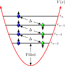
Figure 1: Schematic of the FFLO wave function for a trapped one-dimensional gas Eq. (1) with a population imbalance given by $q=N_{\uparrow}-N_{\downarrow}$. Spin-$\uparrow$ fermions at harmonic oscillator level $n$ are paired with spin-$\downarrow$ fermions at level $n-q$ (our illustration is for the case of $q=1$.) The excess spins-$\uparrow$ occupy low-energy levels with $0\leq n\leq q-1$.

Here, our major interest in the one-dimensional (1D) regime, which has been the subject of extensive recent theoretical work. The theoretical work investigating the FFLO state in 1D has ranged from applying Bethe ansatz Orso2007 ; Hu2007 ; Kakashvili2009 , density-matrix renormalization group Feiguin ; HM2010 ; MolinaPRLComment , quantum Monte Carlo Batrouni , tight binding models BakhtiariPRL2008 ; LuscherPRA2008 , and self-consistent mean-field solutions to the gap equation LiuPRA2007 ; LiuPRA2008 ; Sun2011 ; LuPRL2012 ; SunBolech . Many of these methods only strictly apply to infinite 1D systems, further relying on the uncontrolled local density approximation (LDA) to account for the effects of the trapping potential that is omnipresent in ultracold atomic experiments.

In Ref. SheehyPRA2015 it was shown that a simple variational BCS-type wave function that involved pairing of harmonic-oscillator states could account for pairing correlations in a balanced trapped 1D gas without the necessity of invoking the LDA. Here, we propose a similar wave function for the imbalanced case that incorporates FFLO pairing correlations in a natural way. The wave function is:

$$|\Psi\rangle=\prod_{m=0}^{q-1}\hat{c}^{\dagger}_{m\uparrow}\prod_{n=q}^{\infty}\left(u_{n}+v_{n}\hat{c}^{\dagger}_{n\uparrow}\hat{c}^{\dagger}_{n-q\downarrow}\right)|{\rm vac}\rangle,$$ (1)

where the quantum numbers $(m,n)$ label the discrete energy levels of the trapped gas and the arrow ($\uparrow,\downarrow$) represents the atomic hyperfine state. In the following, the trapping potential will be taken to be harmonic.

This wave function consists of two product factors acting on the vacuum, with the rightmost factor corresponding, physically, to the presence of imbalanced pairing correlations (characterized by the variational parameters $u_{n}$ and $v_{n}$) between a spin-$\uparrow$ fermion at level $n$ and a spin-$\downarrow$ fermion at level $n-q$, as illustrated in Fig. 1. The left most factor corresponds to a central filled core of unpaired spin-$\uparrow$ fermions. This variational wave function has a fixed total population imbalance (or magnetization) equal to $q=N_{\uparrow}-N_{\downarrow}$. In addition, as we shall show below, the real-space local pairing amplitude associated with $|\Psi\rangle$ exhibits the oscillatory real-space pairing correlations expected for an FFLO state. For these reasons, we propose that this is a natural variational wave function to study the FFLO state of a 1D trapped Fermi system.

This paper is organized as follows: In Sec. II, we derive the variational energy equation using Eq. (1) in the harmonic oscillator basis of the trapping potential. Note that we work only in the zero-temperature limit, studying ground-state properties. We further discuss the necessity of allowing the oscillator length scales associated with the single-particle basis to differ from that of the harmonic potential. The energy is then directly minimized numerically, without resorting to explicitly finding the Euler-Lagrange equations. The results of this minimization are presented and analyzed in Sec. 4, in which the density profiles and pairing amplitude are shown, as well as density-density correlations. In Sec. IV we make brief concluding remarks.

Before proceeding to our calculations, we conclude this section by describing our main results. We find that an FFLO state of imbalanced Fermi gases, described by Eq. (1), is stable for sufficiently small magnetization ($q$), with a spatially modulated local pairing amplitude that is analogous to the LO phase of an infinite imbalanced gas, possessing nodes at which $|\Delta(x)|$ vanishes. However, we find that the oscillatory pairing amplitude does not leave any appreciable signature in the local density or local magnetization (density difference, $m(x)=n_{\uparrow}(x)-n_{\downarrow}(x)$), such as a local increase in $m(x)$ near the nodes of $|\Delta(x)|$. Our results for these densities agree qualitatively with experiment and theory based on combining the Bethe ansatz with the LDA LiaoNature2010 , showing an imbalanced central region and a paired (balanced) outer region at the edges of the cloud. With increasing $q$, the FFLO phase becomes unstable (as in three-dimensional imbalanced Fermi gases) to an unpaired Fermi gas phase.

II Variational Energy

We study a one-dimensional imbalanced Fermi gas, a system that has been achieved experimentally using an optical lattice potential to create an array of weakly-coupled tubes LiaoNature2010 ; Revelle2016 . In the limit of large optical lattice depth, it is approximately valid to neglect any intertube coupling and we therefore study a single tube with Hamiltonian

$$H= \sum_{\sigma}\int_{-\infty}^{\infty}{\rm d}x\,\hat{\Psi}^{\dagger}_{\sigma}(x)\left[-\frac{\hbar^{2}}{2m}\frac{d^{2}}{dx^{2}}+V(x)\right]\hat{\Psi}_{\sigma}(x)$$

$$+\lambda\int_{-\infty}^{\infty}{\rm d}x\,\hat{\Psi}^{\dagger}_{\uparrow}(x)\hat{\Psi}^{\dagger}_{\downarrow}(x)\hat{\Psi}_{\downarrow}(x)\hat{\Psi}_{\uparrow}(x),$$ (2)

where $V(x)=\frac{1}{2}m\omega^{2}x^{2}$ is the harmonic trapping potential characterized by the trap frequency $\omega$, and $\lambda=-2\hbar^{2}/(ma_{1{\rm D}})$ with $a_{1{\rm D}}$ being the one-dimensional scattering length OlshaniiPRL1998 . The field operators can be expanded in terms of mode operators $\hat{c}_{n\sigma}$ as

$$\hat{\Psi}_{\sigma}(x)=\sum_{n=0}^{\infty}\psi_{n\sigma}(x)\hat{c}_{n\sigma}$$ (3)

and similarly for $\hat{\Psi}_{\sigma}^{\dagger}(x)$. The single-particle states are taken to be harmonic oscillator wave functions:

$$\psi_{n\sigma}(x)=\frac{1}{\sqrt{2^{n}n!a_{\sigma}\sqrt{\pi}}}e^{-x^{2}/(2a^{2}_{\sigma})}H_{n}(x/a_{\sigma}),$$ (4)

where $H_{n}(x)$ are the Hermite polynomials and $a_{\sigma}$ are effective oscillator length scales.

Crucially, we include $a_{\sigma}$ in the set of variational parameters. Thus, in the presence of interactions, they are in general different from the natural oscillator length $a=\sqrt{\hbar/(m\omega)}$, which is determined by the trapping potential. In Ref. SheehyPRA2015 the balanced case was studied using a similar variational wave function. It was found that including this additional variational parameter was necessary to allow the cloud size to decrease with increasing strength of attraction (which is what is expected on physical grounds and is observed experimentally).

Similarly, in the imbalanced case, we allow the oscillator lengths to be variational parameters to obtain realistic density profiles. As discussed below, we find, in the imbalanced regime, that the optimal (minimal energy) values of the spin-$\uparrow$ and spin-$\downarrow$ oscillator lengths generally satisfy (for attractive interactions) $a_{\sigma}<a$ and $a_{\uparrow}<a_{\downarrow}$. This imples that interaction effects cause the two fermion species to each feel an effective trapping potential with a frequency that is larger than the actual trap frequency, with the majority species trap frequency slightly larger than that of the minority species.

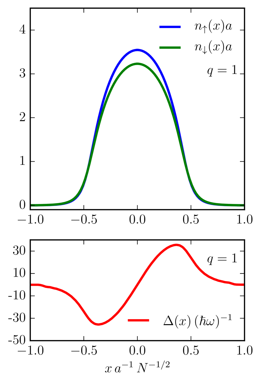
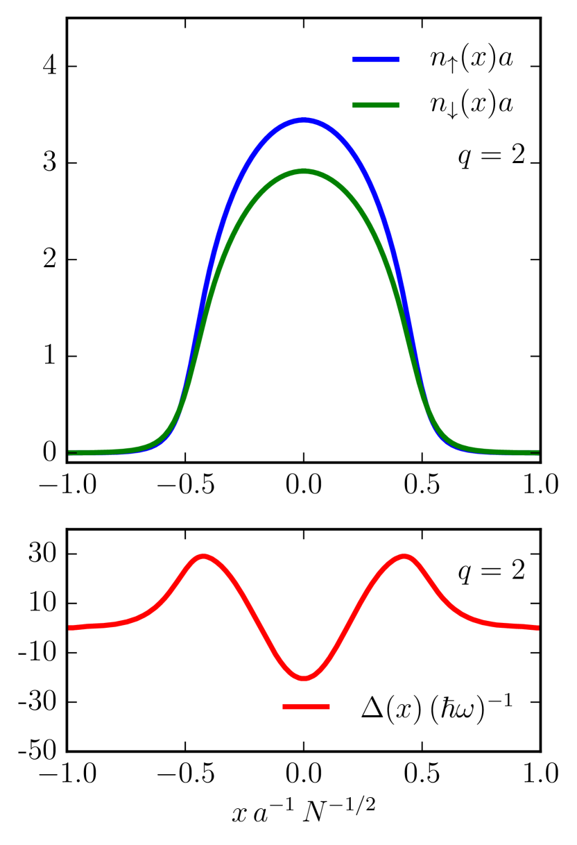
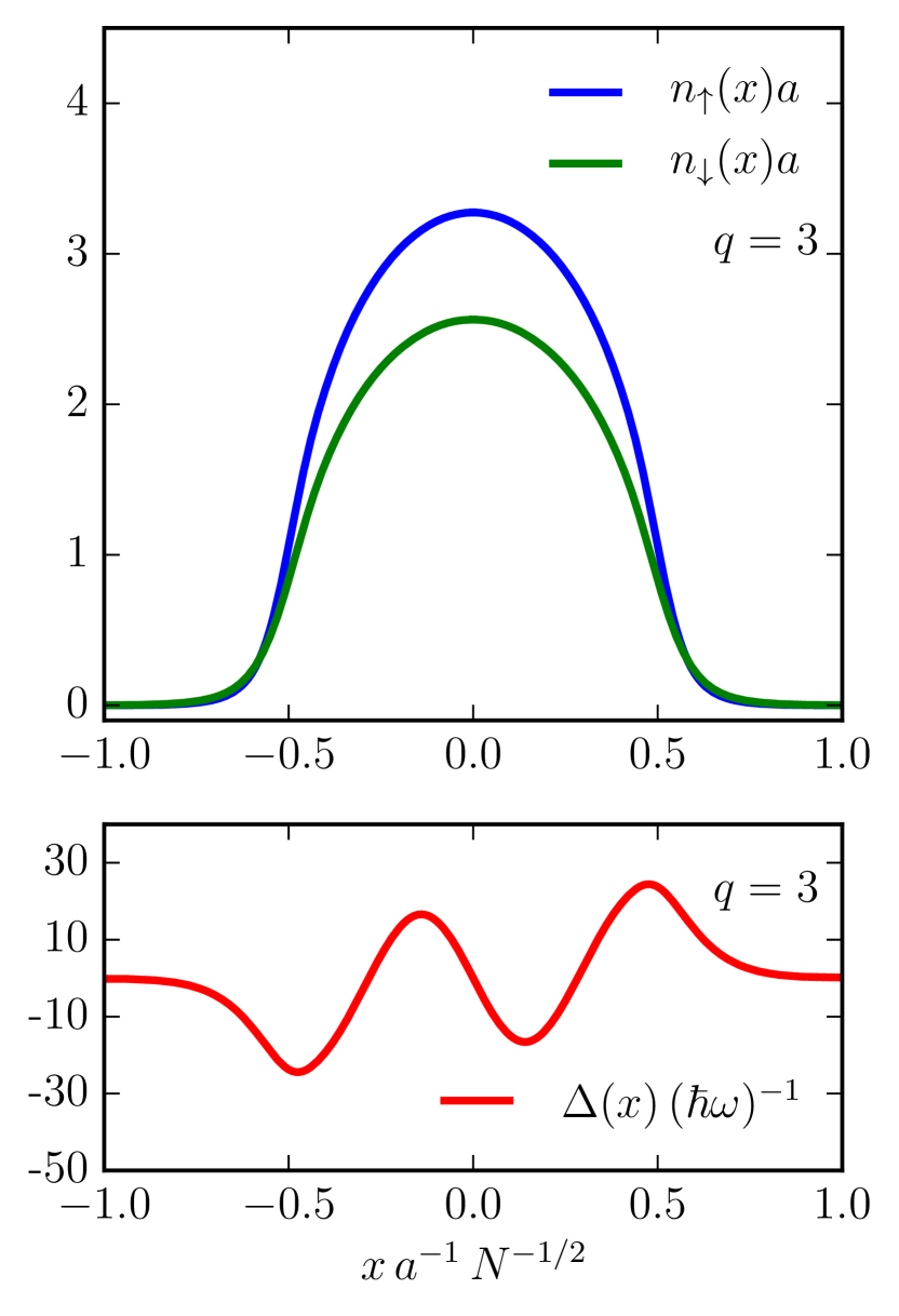
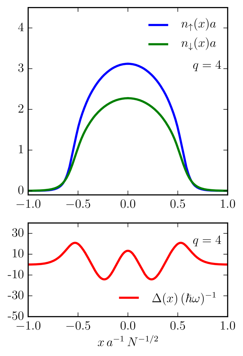
Figure 2: (Color Online) The top row shows the spin-resolved densities, given by Eqs. (12), of a trapped strongly interacting imbalanced fermion gas for various magnetizations $q=M=N_{\uparrow}-N_{\downarrow}$. Note that $n_{\uparrow}(x)\geq n_{\downarrow}(x)$ always. Here, $a=\sqrt{\hbar/(m\omega)}$ is the harmonic oscillator length scale of the trapping potential. The total particle number $N=N_{\uparrow}+N_{\downarrow}\approx 25$. As the polarization $P=q/N$ increases from about $P=0.02$ for $q=1$ to $P=0.08$ for $q=4$ the size of the central locally magnetized region of the could increases. The bottom row shows the local pairing amplitude Eq. (13) for the respective values of $q$. For each additional unpaired spin a node appears in $\Delta(x)$. This oscillatory structure is a signature of the FFLO state.

With $a_{\sigma}\neq a$ the single-particle states, Eq. (4), are no longer eigenstates of the kinetic energy term of the Hamiltonian, Eq. (II). However, it is still straightforward to use the properties of the harmonic oscillator wavefunctions to express the Hamiltonian in terms of the mode operators $\hat{c}_{n\sigma}$. In performing this step, it is convenient to express the trapping potential as $V(x)=\frac{1}{2}m\omega^{2}_{\sigma}x^{2}+\frac{1}{2}m(\omega^{2}-\omega^{2}_{\sigma})x^{2}$ with $\omega_{\sigma}=\hbar/(ma_{\sigma}^{2})$ the effective trap associated with the variational oscillator lengths. In terms of mode operators the Hamiltonian can then be expressed as

$$H= \sum_{n,\sigma}\epsilon_{n\sigma}\hat{c}^{\dagger}_{n\sigma}\hat{c}_{n\sigma}+\sum_{\{n_{i}\}}\lambda^{\uparrow,\downarrow}_{n_{1},n_{2},n_{3},n_{4}}\hat{c}^{\dagger}_{n_{1}\uparrow}\hat{c}^{\dagger}_{n_{2}\downarrow}\hat{c}_{n_{3}\downarrow}\hat{c}_{n_{4}\uparrow},$$ (5)

where $\epsilon_{n\sigma}=\frac{\hbar\omega}{2}(n+1/2)(\ell^{2}_{\sigma}+\ell^{-2}_{\sigma})$ with $\ell_{\sigma}=a_{\sigma}/a$, and

$$\lambda^{\uparrow,\downarrow}_{n_{1},n_{2},n_{3},n_{4}}=\lambda\int_{-\infty}^{\infty}{\rm d}x\,\psi^{*}_{n_{1}\uparrow}(x)\psi^{*}_{n_{2}\downarrow}(x)\psi_{n_{3}\downarrow}(x)\psi_{n_{4}\uparrow}(x).$$ (6)

In Eq. (5), the summations over the integers $n$ and $n_{i}$ are from $0$ to $\infty$. A convenient expression for Eq. (6), expressed in terms of a sum over integers, is given in the Appendix. Note, in Eq. (5) we have dropped off-diagonal terms in the kinetic energy, as our variational wave function, Eq. (1), does not connect states having different principal quantum numbers, i.e., $\langle\Psi|\hat{c}^{\dagger}_{n\sigma}\hat{c}_{n^{\prime}\sigma}|\Psi\rangle=0$ for $n\neq n^{\prime}$.

Our variational wave function, Eq. (1), has a definite value of the magnetization $q=M=N_{\uparrow}-N_{\downarrow}$ but an uncertain value of the total particle number (as does the usual BCS wave function). Therefore, we proceed by minimizing the grand-canonical energy

$${\cal E}=\langle H\rangle-\mu\langle\hat{N}\rangle,$$ (7)

with the chemical potential $\mu$, a Lagrange multiplier, that fixes the average total particle number. Upon evaluating the expectation value and dropping irrelevant constant terms we find for the grand-canonical energy:

$${\cal E}(\{v_{n},u_{n}\},\ell_{\sigma})=\frac{\hbar\omega}{4}(\ell^{2}_{\uparrow}+\ell^{-2}_{\uparrow})q^{2}$$ (8)

$$+\sum_{n=q}^{\infty}\big{[}\epsilon_{n\uparrow}+\epsilon_{n-q\downarrow}-2\mu+\bar{\bar{\lambda}}^{\uparrow,\downarrow}_{n}(q)\big{]}|v_{n}|^{2}$$

$$+\sum_{n=q}^{\infty}\sum_{n^{\prime}=0}^{\infty}\lambda^{\uparrow,\downarrow}_{n,n^{\prime}}|v_{n}|^{2}|v_{n^{\prime}+q}|^{2}+\sum_{n,n^{\prime}=q}^{\infty}\bar{\lambda}^{\uparrow,\downarrow}_{n,n^{\prime}}(q)u^{*}_{n}v_{n}u_{n^{\prime}}v^{*}_{n^{\prime}},$$

where for notational convenience we have defined

$$\lambda^{\uparrow,\downarrow}_{n,n^{\prime}} \equiv \lambda^{\uparrow,\downarrow}_{n,n^{\prime},n^{\prime},n},$$ (9a)

$$\bar{\lambda}^{\uparrow,\downarrow}_{n,n^{\prime}}(q) \equiv \lambda^{\uparrow,\downarrow}_{n,n-q,n^{\prime}-q,n^{\prime}},$$ (9b)

$$\bar{\bar{\lambda}}^{\uparrow,\downarrow}_{n}(q) \equiv \sum_{m=0}^{q-1}\sum_{m^{\prime}=0}^{q-1}\lambda^{\uparrow,\downarrow}_{m,n-q,n-q,m^{\prime}}.$$ (9c)

We see that the coupling function appears in three places in the grand-canonical energy function. The term containing $\bar{\bar{\lambda}}^{\uparrow,\downarrow}_{n}$ in the second line of Eq. (8) describes a Hartree interaction between the paired and unpaired atoms. In the third line of Eq. (8), the term containing $\lambda^{\uparrow,\downarrow}_{n,n^{\prime}}$ describes the pairing interaction, and the term containing $\bar{\lambda}^{\uparrow,\downarrow}_{n,n^{\prime}}(q)$ describes the Hartree interaction among the paired atoms.

Instead of further proceeding to obtain the Euler-Lagrange equations from Eq. (8) we will seek to numerically minimize the ground state energy directly with respect to the parameters $v_{n}$, $u_{n}$, and $a_{\sigma}$ (or $\ell_{\sigma}$), with the chemical potential adjusted to yield the correct particle number via

$$N=\langle\hat{N}\rangle=-\frac{\partial{\cal E}}{\partial\mu}.$$ (10)

Once the optimum values of the parameters are known, all other ground state properties can be obtained, e.g., densities, pairing amplitude, etc. To this end, with the constraint $|v_{n}|^{2}+|u_{n}|^{2}=1$, it will be useful to parameterize $v_{n}=\cos(\theta_{n})$ and $u_{n}=\sin(\theta_{n})$. The ground state energy can then be written as

$${\cal E}(\{\theta_{n}\},\ell_{\sigma})=\frac{\hbar\omega}{4}(\ell^{2}_{\uparrow}+\ell^{-2}_{\uparrow})q^{2}$$

$$+\sum_{n=q}^{\infty}\big{[}\epsilon_{n\uparrow}+\epsilon_{n-q\downarrow}-2\mu+\bar{\bar{\lambda}}^{\uparrow,\downarrow}_{n}(q)\big{]}\cos^{2}(\theta_{n})$$

$$+\sum_{n=q}^{\infty}\sum_{n^{\prime}=0}^{\infty}\lambda^{\uparrow,\downarrow}_{n,n^{\prime}}\cos^{2}(\theta_{n})\cos^{2}(\theta_{n^{\prime}+q})$$

$$+\sum_{n,n^{\prime}=q}^{\infty}\bar{\lambda}^{\uparrow,\downarrow}_{n,n^{\prime}}(q)\sin(\theta_{n})\cos(\theta_{n})\sin(\theta_{n^{\prime}})\cos(\theta_{n^{\prime}}).$$ (11)

To numerically minimize Eq. (II) with respect to the set of angles $\theta_{n}$ and normalized oscillator lengths $\ell_{\sigma}$ an upper cutoff to the number of oscillators levels included has to be set. For each coupling strength and particle number we choose a large enough cutoff such that the final results are insensitive to this value. In the next section, we describe our results.

III Results

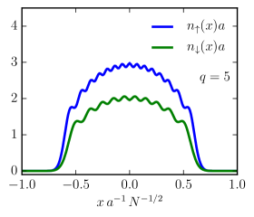
Figure 3: (Color Online) Density profiles for spin-$\uparrow$ and spin-$\downarrow$ for $q=5$ and $N=25$, in the regime of $P>P_{c}$ where the unpaired state has lower energy than the paired state, so that $\Delta(x)=0$. Note that $n_{\uparrow}(x)>n_{\downarrow}(x)$ for all $x$.

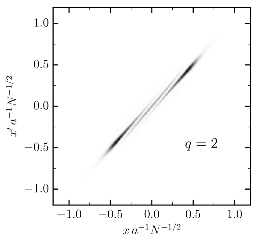
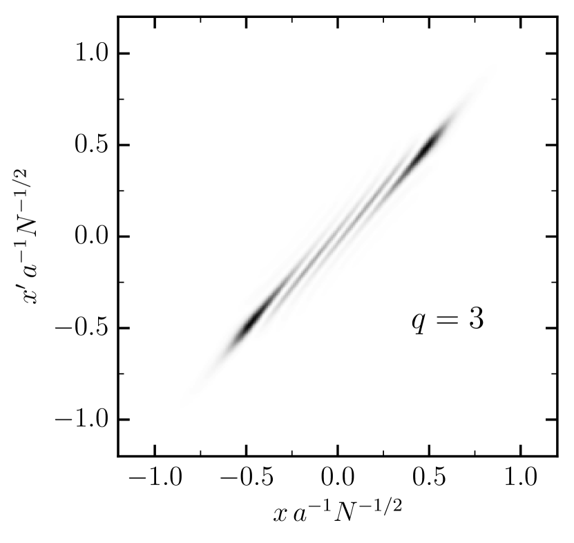
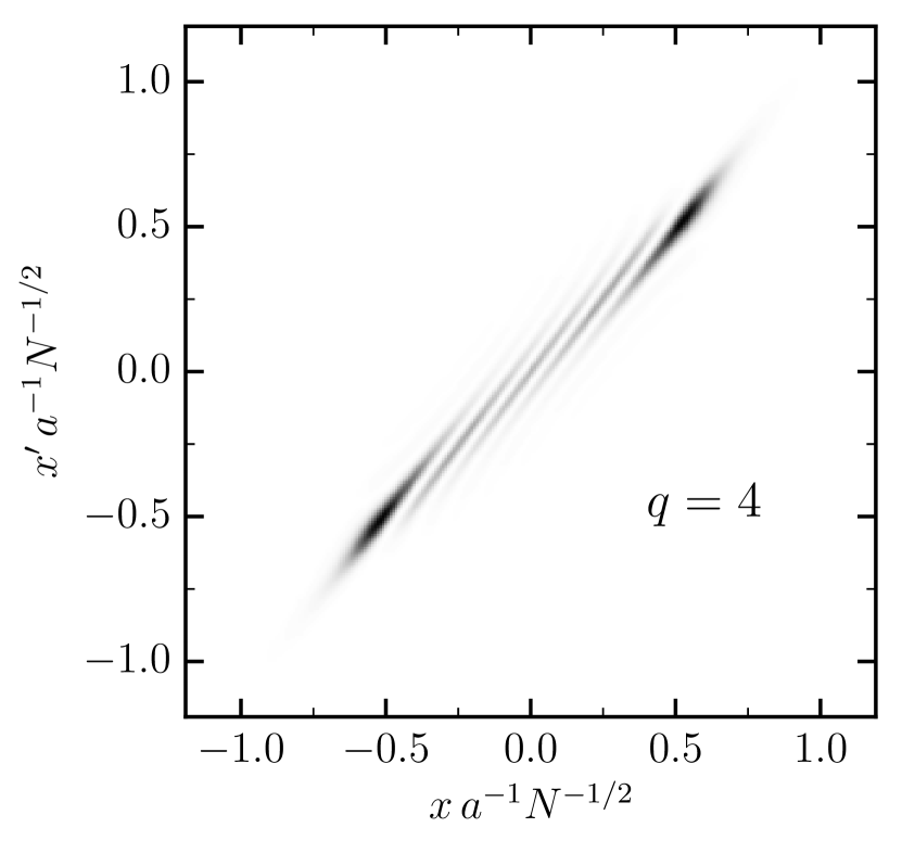
Figure 4: Real space (in situ) density-density correlations Eq. (III) for various values of the imbalance $q$. The two large “peaks” in each correspond to the regions shown in Fig. 2 where the spin-$\uparrow$ and spin-$\downarrow$ densities are approximately equal. The oscillations between these regions are related to FFLO correlations. Cross-sections along the diagonal of each of these plots are shown in Fig. 5

The spin-resolved local densities $n_{\sigma}(x)=\langle\hat{\Psi}^{\dagger}_{\sigma}(x)\hat{\Psi}_{\sigma}(x)\rangle$ are typical observables in ultracold atomic systems, where the expectation value is with respect to Eq. (1). The local densities are:

$$n_{\uparrow}(x) =\sum_{n=0}^{q-1}|\psi_{n\uparrow}(x)|^{2}+\sum_{n=q}^{\infty}|\psi_{n\uparrow}(x)|^{2}|v_{n}|^{2},$$ (12a)

$$n_{\downarrow}(x) =\sum_{n=q}^{\infty}|\psi_{n-q\downarrow}(x)|^{2}|v_{n}|^{2},$$ (12b)

with the first (second) term of Eq. (12a) being the density of unpaired (paired) majority species (i.e., spin-$\uparrow$) fermions. Within our variational ansatz, all spins-$\downarrow$ are pairied, as seen in Eq. (12b). Note that $n_{\uparrow}(x)$ and $n_{\downarrow}(x)$ depend on the variational parameters $v_{n}$ but also on $a_{\uparrow}$ and $a_{\downarrow}$ via the oscillator wavefunctions. Similarly, the local pairing amplitude $\Delta(x)=-\lambda\langle\hat{\Psi}_{\downarrow}(x)\hat{\Psi}_{\uparrow}(x)\rangle$ is

$$\Delta(x)=-\lambda\sum_{n=q}^{\infty}\psi_{n-q\downarrow}(x)\psi_{n\uparrow}(x)u_{n}v_{n}.$$ (13)

Although it is not directly measurable, the magnitude of $\Delta(x)$ measures the strength of the local pairing (and the local single-particle gap).

The top row of Fig. 2 shows the obtained local density profiles for various values of the total magnetization $q$, while the bottom row shows the local pairing amplitude that, as expected for an FFLO state, is oscillatory in real space. The other system parameters are $\lambda=-20\,\hbar\omega a$ and $N\approx 25$, so that the dimensionless interaction parameter $Na^{2}_{\rm 1D}/a^{2}\approx 0.25$, which corresponds to the strongly interacting regime Orso2007 and the approximate value in recent experiments LiaoNature2010 . As can be seen, the central region of the cloud is magnetized, while at the edges of the cloud the two densities remain approximately equal. The size of this imbalanced region increases with increasing polarization $P=q/N$.

The same behavior for the density profiles, i.e., an imbalanced central region and balanced outer region, was seen in the experimental results of Ref.LiaoNature2010 and found to be consistent with a theoretical analysis based on combining Bethe ansatz with the LDA. Within such a theoretical description, the observed density profiles are interpreted in terms of the cloud being in a locally imbalanced phase in the center and in a locally paired phase at the edges.

$q$	$a_{\uparrow}/a$	$a_{\downarrow}/a$
1	0.45	0.47
2	0.47	0.51
3	0.51	0.57
4	0.55	0.64

Table 1: Spin-dependent oscillator lengths normalized to the oscillator length set by the trapping potential $a$ for various values of the total magnetization $q$.

Since our calculations do not make use of the LDA, we instead interpret our density profiles as arising from the system being in the FFLO state described by Eq. (1). To understand why the edges are locally paired, we note that the result of minimizing Eq. (II) yields the variational parameters $u_{n}$ and $v_{n}$ but also the oscillator length variational parameters, which we display in Table 1. These results show that the effective oscillator lengths ($a_{\uparrow}$ and $a_{\downarrow}$) are significantly smaller than the real system oscillator length, representing the expected contraction of the cloud due to the attractive interactions. In addition, $a_{\uparrow}<a_{\downarrow}$, so that the spins-$\downarrow$ contract somewhat less than the spins-$\uparrow$ (with a difference that increases with increasing imbalance). By entering a ground state with $a_{\uparrow}<a_{\downarrow}$, our system is effectively allowing the minority spin-cloud to expand relative to the majority spin-cloud, so that the system is locally balanced (which favors pairing) at the edges of the cloud, as seen in Fig. 2.

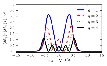
Figure 5: (Color Online) Cross sections of Fig. 4 along the diagonal $x=x^{\prime}$ of the in situ density-density correlation function Eq. (III). Note that the $q=1$ case possesses the largest magnitude, and the $q=4$ case the smallest. This observable measures the square of the pairing amplitude shown in Fig. 2, directly revealing the FFLO pairing oscillations.

Although the pairing amplitude shows oscillatory behavior in real space, with nodes reminiscent of the LO phase (with the number of nodes equal to $q$), no discernable signature of the pairing oscillations is reflected in the spin resolved densities. We also find that the FFLO state is only stable for sufficiently small $q$, reflecting a critical polarization $P_{\rm c}$ above which the unpaired Fermi-gas state becomes energetically favored. For $\lambda=-20\,\hbar\omega a$ this occurs for $q>4$ ($P_{\rm c}=0.16$) with $N=25$ and $q>2$ ($P_{\rm c}=0.04$) with $N=50$. Figure 3 shows the densities of the two spin states for the case of $q=5$, above the critical polarization. The small wiggles in the curves are due to the harmonic oscillator wavefunctions comprising the imbalanced Fermi gas ground state (since, within our theory, this phase is essentially an imbalanced Fermi gas state). Henceforth we concentrate on the FFLO phase and leave mapping the phase diagram for future work.

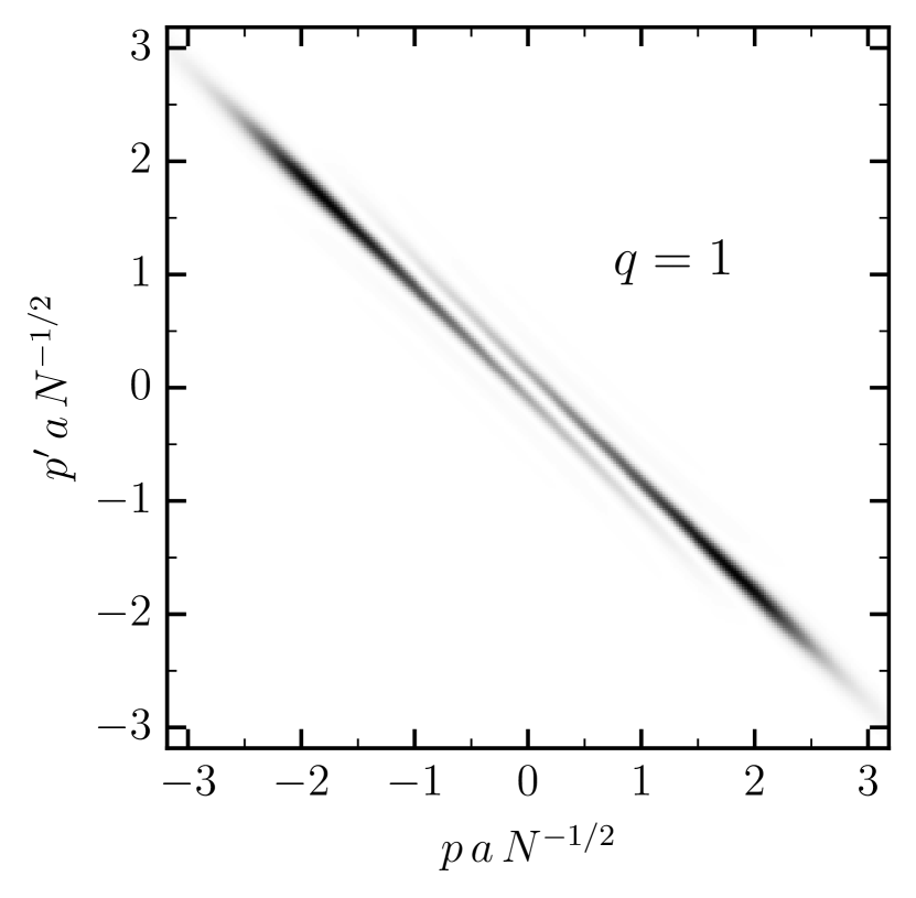
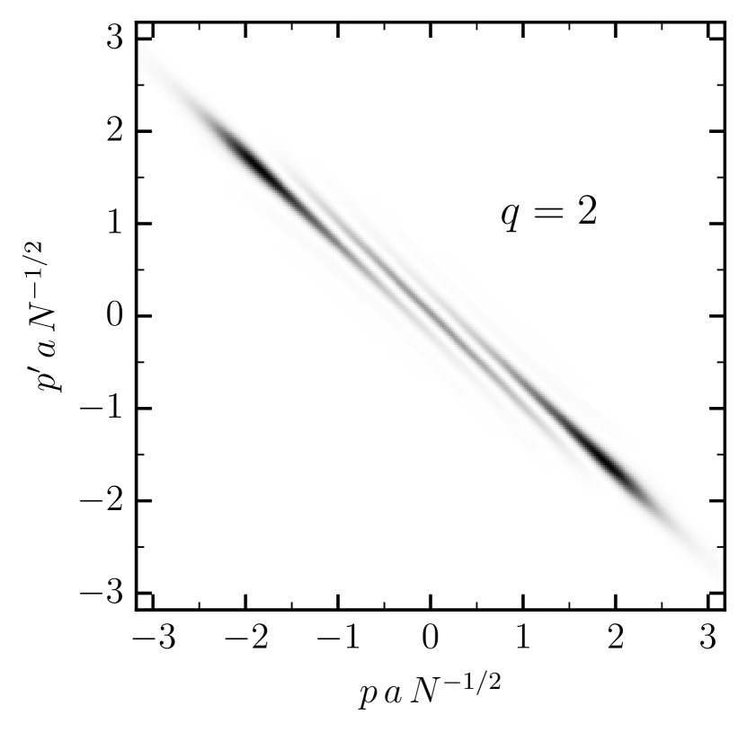
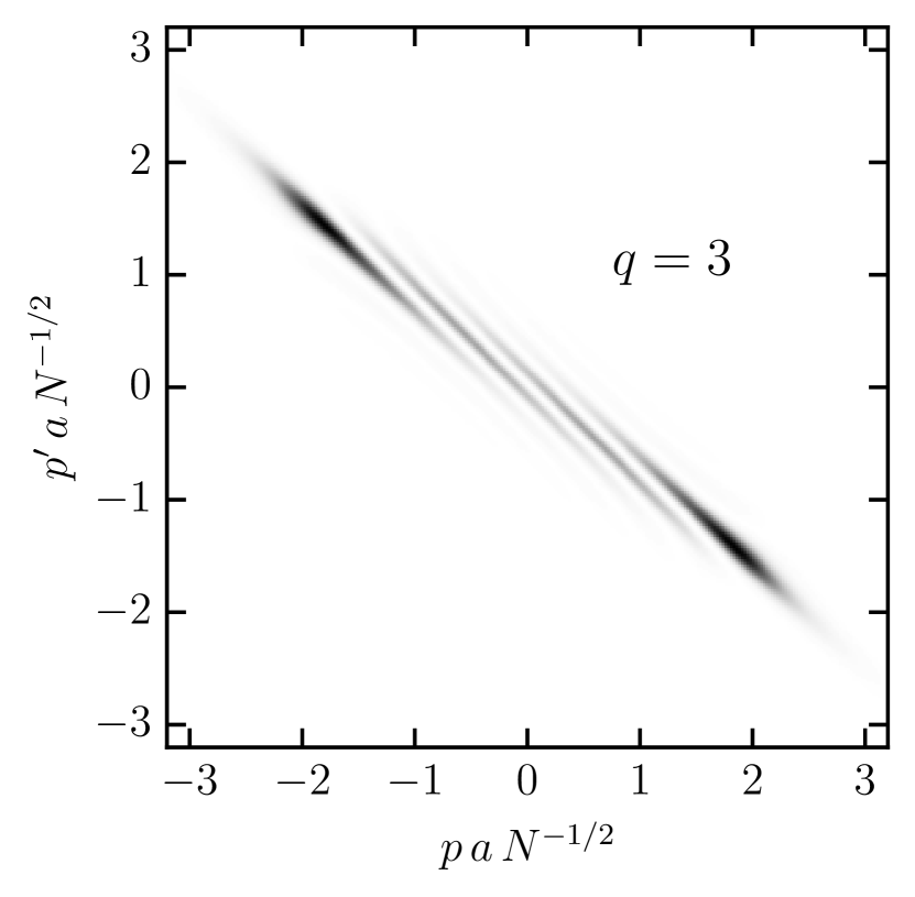
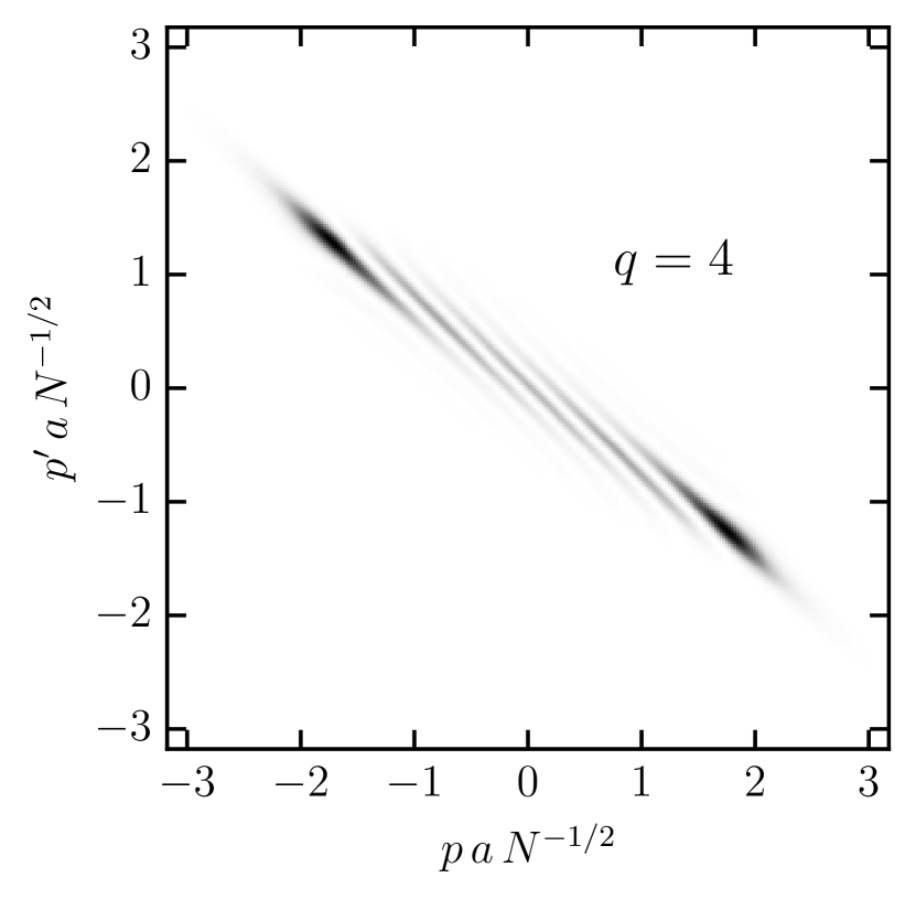
Figure 6: Density-density correlations in momentum space (probed by measuring the real-space density correlations after free expansion Altman04 ; Greiner05 ), Eq. (III), for various imbalances. The two peaks correspond to Cooper-paired states $(k_{{\rm F}\uparrow},-k_{{\rm F}\downarrow})$ and $(-k_{{\rm F}\uparrow},k_{{\rm F}\downarrow})$ or $(k_{{\rm F}\uparrow},Q-k_{{\rm F}\uparrow})$ and $(-k_{{\rm F}\uparrow},k_{{\rm F}\uparrow}-Q)$, where $Q$ is the momentum of the FFLO pair.

We now turn to the question of how to directly probe the 1D FFLO state in an experiment via density-density correlations. Density-density correlations can be performed after free expansion Altman04 ; Greiner05 and in situ HungNJP . We first investigate the latter for our system. Figure 4 shows the equal-time in situ density correlations defined as

$$\Pi(x,x^{\prime}) =\langle\delta\hat{n}_{\uparrow}(x)\delta\hat{n}_{\downarrow}(x)\rangle,$$

$$=\left|\sum_{n=q}^{\infty}\psi_{n-q\downarrow}(x)\psi_{n\uparrow}(x^{\prime})u_{n}v_{n}\right|^{2},$$ (14)

where $\delta\hat{n}_{\sigma}(x)=\hat{n}_{\sigma}(x)-\langle\hat{n}_{\sigma}(x)\rangle$, for various imbalances and the same parameters as Fig. 2.

The two highly correlated regions seen in each plot of Fig. 4 correspond to the edges of the cloud where the spin-$\uparrow$ and spin-$\downarrow$ densities are approximately equal, seen in Fig. 2. In between these regions the correlations show an oscillatory behavior. In fact, along the diagonal $\Pi(x,x)\propto|\Delta(x)|^{2}$. Thus, the square of the pairing amplitude can be directly probed, explicitly revealing the FFLO oscillations. Figure 5 shows cross-sections of the density-density correlations along $x=x^{\prime}$ for each plot of Fig. 4, unambiguously showing the modulated pairing amplitude that is characteristic of the FFLO state.

Next we turn to momentum correlations in the trapped FFLO state, which has a similar experimental signature. Assuming inter-particle interactions can be neglected during the expansion LuPRL2012 , measuring the density after releasing the trapping potential and allowing the gas to freely expand probes the momentum distribution $\langle\hat{n}_{\sigma}(k)\rangle$, where $\hat{n}_{\sigma}(k)=\hat{c}^{\dagger}_{k\sigma}\hat{c}_{k\sigma}$ and $\hat{c}^{(\dagger)}_{k\sigma}$ annihilates (creates) single-particle plane wave states having momentum $k$. The noise correlations of such a measurement are proportional to the momentum-space density correlations Altman04 ; Greiner05 . Figure 6 shows the equal-time momentum-space density correlation function

$$C(k,k^{\prime}) =\langle\delta\hat{n}_{\uparrow}(k)\delta\hat{n}_{\downarrow}(k^{\prime})\rangle$$

$$\propto\left|\sum_{n=q}^{\infty}\psi_{n-q\downarrow}(k)\psi_{n\uparrow}(k^{\prime})u_{n}v_{n}\right|^{2},$$ (15)

where $\delta\hat{n}_{\sigma}(k)=\hat{n}_{\sigma}(k)-\langle\hat{n}_{\sigma}(k)\rangle$ and $\psi_{n\sigma}(k)$ is the Fourier transform of the harmonic oscillator states, Eq. (4), for various imbalances and the same parameters as Fig. 2.

As one might expect, the largest correlations are along the anti-diagonal $k=-k^{\prime}$. The two regions of each graph showing the highest correlations correspond to momentum states near the Fermi surfaces (points in one-dimension): $(k_{{\rm F}\uparrow},-k_{{\rm F}\downarrow})$ and $(-k_{{\rm F}\uparrow},k_{{\rm F}\downarrow})$ or in terms of the momentum of the FFLO Cooper-pair $Q$ $(k_{{\rm F}\uparrow},Q-k_{{\rm F}\uparrow})$ and $(-k_{{\rm F}\uparrow},k_{{\rm F}\uparrow}-Q)$. Therefore because of the Fermi surface mismatch in an imbalanced system the two regions of highest correlations are off-set from the anti-diagonal by amount approximately given by the momentum of the Cooper pairs. Unlike the in situ density correlations that can give information about the local pairing amplitude, the momentum correlations gives information about the momentum of the Cooper pairs. Taking together they provide unambiguous signatures of two related predictions of the FFLO state.

IV Conclusion

Superconductivity, or fermionic superfluidity in the presence of a population imbalance existing beyond the Chandrasekhar-Clogston limit has been a topic of interest for many decades. A long-sought-after candidate, the FFLO state, has been very elusive. Ultracold atomic gases provide an almost ideal system to produce such exotic superfluid states because the particle number, interactions, dimensionally can all be externally controlled. In these systems the inhomogeneity caused by the trapping potential can have nontrivial effects. To this end, here we have proposed a ground-state variational BCS-like wave function for an imbalanced system that explicitly takes into account the effects of the trapping potential without relying on the local density approximation.

We find that FFLO type pairing is only stable for relatively small values of the polarization $P=q/N$, with an imbalanced unpaired phase stable at larger $P$. In the small $P$ regime where the FFLO is stable, we find density profiles that, while qualitatively consistent with experiments LiaoNature2010 , do not show any signature of FFLO pairing correlations in the density. However, we find that two-particle correlations (such as the in situ and free expansion density-density correlations) show clear experimental signatures of the local pairing oscillations and finite Cooper pair momentum of an FFLO superfluid.

*

Appendix A Interaction matrix elements

In this section we provide simplified expressions for the various interaction matrix elements required for our calculations. Our starting point is the interfermion interaction Eq. (6):

$$\lambda^{\uparrow,\downarrow}_{n_{1},n_{2},n_{3},n_{4}}=\lambda\int_{-\infty}^{\infty}{\rm d}x\,\psi^{*}_{n_{1}\uparrow}(x)\psi^{*}_{n_{2}\downarrow}(x)\psi_{n_{3}\downarrow}(x)\psi_{n_{4}\uparrow}(x),$$ (16)

where

$$\psi_{n\sigma}(x)=\frac{1}{\sqrt{2^{n}n!a_{\sigma}\sqrt{\pi}}}e^{-z^{2}/(2a^{2}_{\sigma})}H_{n}(x/a_{\sigma}),$$ (17)

are harmonic oscillator states (or Hermite functions) with spin dependent oscillator lengths $a_{\sigma}$. Henceforth, we shall drop the integration limits, with the understanding that they are always from $-\infty$ to $\infty$. Plugging in $\psi_{n\sigma}(x)$ leads to:

$$\lambda^{\uparrow,\downarrow}_{n_{1},n_{2},n_{3},n_{4}}=\frac{\lambda}{\pi a_{\uparrow}a_{\downarrow}}\frac{1}{\sqrt{2^{n_{1}+n_{2}+n_{3}+n_{4}}n_{1}!n_{2}!n_{3}!n_{4}!}}$$

$$\times\int{\rm d}x\,e^{-2x^{2}/\bar{a}^{2}}H_{n_{1}}(x/a_{\uparrow})H_{n_{2}}(x/a_{\downarrow})H_{n_{3}}(x/a_{\downarrow})$$

$$\hskip 71.13188pt\times H_{n_{4}}(x/a_{\uparrow}),$$ (18)

where

$$\bar{a}^{2}=\frac{2}{\frac{1}{a^{2}_{\uparrow}}+\frac{1}{a^{2}_{\downarrow}}},$$ (19)

is the harmonic mean of the square of the oscillator lengths. Recasting the integral into dimensionless form by defining $u=x/\bar{a}$ we have

$$\lambda^{\uparrow,\downarrow}_{n_{1},n_{2},n_{3},n_{4}}=\frac{\lambda\bar{a}}{\pi a_{\uparrow}a_{\downarrow}}\frac{1}{\sqrt{2^{n_{1}+n_{2}+n_{3}+n_{4}}n_{1}!n_{2}!n_{3}!n_{4}!}}$$

$$\times\int{\rm d}u\,e^{-2u^{2}}H_{n_{1}}(u\bar{a}/a_{\uparrow})H_{n_{2}}(u\bar{a}/a_{\downarrow})H_{n_{3}}(u\bar{a}/a_{\downarrow})$$

$$\hskip 56.9055pt\times H_{n_{4}}(u\bar{a}/a_{\uparrow}).$$ (20)

Thus we need to evaluate the following integral:

$$I=\int{\rm d}u\,e^{-2u^{2}}H_{n_{1}}(u\bar{a}/a_{\uparrow})H_{n_{2}}(u\bar{a}/a_{\downarrow})H_{n_{3}}(u\bar{a}/a_{\downarrow})$$

$$\hskip 64.01869pt\times H_{n_{4}}(u\bar{a}/a_{\uparrow}).$$ (21)

In principle this integral can be express in terms of a Lauricella function of the second kind Lord1948 , but this is still computationally inefficient to evaluate. Thus, we use the Feldheim relation for the product of two Hermite polynomials

$$H_{m}(z)H_{n}(z)=m!n!\sum_{\nu=0}^{{\rm min}(m,n)}\frac{2^{\nu}H_{m+n-2\nu}(z)}{\nu!(m-\nu)!(n-\nu)!},$$ (22)

to arrive at

$$I= n_{1}!n_{2}!n_{3}!n_{4}!\sum_{\nu_{1}=0}^{{\rm min}(n_{1},n_{4})}\sum_{\nu_{2}=0}^{{\rm min}(n_{2},n_{3})}\frac{2^{\nu_{1}}}{\nu_{1}!(n_{1}-\nu_{1})!(n_{4}-\nu_{1})!}$$

$$\times\frac{2^{\nu_{2}}}{\nu_{2}!(n_{2}-\nu_{2})!(n_{3}-\nu_{2})!}$$

$$\times\int{\rm d}u\,e^{-2u^{2}}H_{n_{1}+n_{4}-2\nu_{1}}(u\bar{a}/a_{\uparrow})H_{n_{2}+n_{3}-2\nu_{2}}(u\bar{a}/a_{\downarrow}).$$ (23)

Next we use the following integral identity Lord1948

$$2^{-1/2}\int{\rm d}ue^{-u^{2}}H_{m}(u\alpha)H_{n}(u\beta)=$$

$$\begin{cases}(-1)^{\frac{1}{2}(m-n)}2^{m+n-\frac{1}{2}}\alpha^{n}\beta^{m}\Gamma\left(\frac{m+n+1}{2}\right)&\text{if }m+n\text{ is even}\\ 0&\text{otherwise},\end{cases}$$ (24)

which holds if $\alpha^{2}+\beta^{2}=1$. With this, we have

$$\lambda^{\uparrow,\downarrow}_{n_{1},n_{2},n_{3},n_{4}}= \frac{\lambda\bar{a}}{\pi a_{\uparrow}a_{\downarrow}}\sqrt{\frac{n_{1}!n_{2}!n_{3}!n_{4}!}{2^{n_{1}+n_{2}+n_{3}+n_{4}}}}\sum_{\nu_{1}=0}^{\min(n_{1},n_{4})}\sum_{\nu_{2}=0}^{\min(n_{2},n_{3})}\frac{2^{\nu_{1}}}{\nu_{1}!(n_{1}-\nu_{1})!(n_{4}-\nu_{1})!}\frac{2^{\nu_{2}}}{\nu_{2}!(n_{2}-\nu_{2})!(n_{3}-\nu_{2})!}$$

$$\times J^{\uparrow,\downarrow}_{n_{1}+n_{4}-2\nu_{1},n_{2}+n_{3}-2\nu_{2}},$$ (25)

where

$$J^{\uparrow,\downarrow}_{m,n}=\begin{cases}\displaystyle(-1)^{\frac{1}{2}(m-n)}2^{m/2+n/2-1/2}\left(\frac{\bar{a}}{a_{\uparrow}}\right)^{n}\left(\frac{\bar{a}}{a_{\downarrow}}\right)^{m}\Gamma\left(\frac{m+n+1}{2}\right)&\text{if }m+n\text{ is even}\\ 0&\text{otherwise}.\end{cases}$$ (26)

Thus, we have expressed the integration of a product of four Hermite functions (with distinct oscillator lengths), Eq. (6), as a double sum over integers.

From this general result, further simplification can be achieved for the three special cases that are needed in Eq. (9) $\lambda^{\uparrow,\downarrow}_{n,n^{\prime}}$, $\bar{\lambda}^{\uparrow,\downarrow}_{n,n^{\prime}}(q)$, and $\bar{\bar{\lambda}}^{\uparrow,\downarrow}_{n}(q)$, corresponding to pairing interactions, Hartree interactions among pairs, and Hartree interactions between the pairs and excess spins-$\uparrow$, respectively.

A.1 Pairing interaction: $\lambda^{\uparrow,\downarrow}_{n,n^{\prime}}\equiv\lambda^{\uparrow,\downarrow}_{n,n^{\prime},n^{\prime},n}$

In this limit Eq. (A) simplifies to

$$\lambda^{\uparrow,\downarrow}_{n,n^{\prime}}= \frac{\lambda}{\sqrt{2}\pi\bar{a}}\frac{n!}{n^{\prime}!}(-1)^{n-n^{\prime}}\left(\frac{\bar{a}}{a_{\uparrow}}\right)^{2n^{\prime}+1}\left(\frac{\bar{a}}{a_{\downarrow}}\right)^{2n+1}\sum_{\nu_{1}=0}^{n}\frac{(-1)^{-\nu_{1}}\Gamma\left(n+n^{\prime}-\nu_{1}+\tfrac{1}{2}\right)}{\nu_{1}![(n-\nu_{1})!]^{2}}\left(\frac{a_{\downarrow}}{\bar{a}}\right)^{2\nu_{1}}$$

$$\times{}_{2}F_{1}\left(-n^{\prime},-n^{\prime};\tfrac{1}{2}-n-n^{\prime}+\nu_{1};a^{2}_{\uparrow}/\bar{a}^{2}\right),$$ (27)

where ${}_{2}F_{1}(a,b;c;x)$ is a hypergeometric function.

A.2 Hartree interaction among pairs: $\bar{\lambda}^{\uparrow,\downarrow}_{n,n^{\prime}}(q)\equiv\lambda^{\uparrow,\downarrow}_{n,n-q,n^{\prime}-q,n^{\prime}}$

In this limit Eq. (A) simplifies to

$$\bar{\lambda}^{\uparrow,\downarrow}_{n,n^{\prime}}(q)= \frac{\lambda(-1)^{q}}{\sqrt{2}\pi\bar{a}}\sqrt{\frac{n!n^{\prime}!}{(n-q)!(n^{\prime}-q)!}}\left(\frac{\bar{a}}{a_{\uparrow}}\right)^{n+n^{\prime}-2q+1}\left(\frac{\bar{a}}{a_{\downarrow}}\right)^{n+n^{\prime}+1}\sum_{\nu_{1}=0}^{\min(n,n^{\prime})}\frac{(-1)^{-\nu_{1}}\Gamma\left(n+n^{\prime}-q-\nu_{1}+\tfrac{1}{2}\right)}{\nu_{1}!(n-\nu_{1})!(n^{\prime}-\nu_{1})!}\left(\frac{a_{\downarrow}}{\bar{a}}\right)^{2\nu_{1}}$$

$$\times{}_{2}F_{1}\left(-n+q,-n^{\prime}+q;\tfrac{1}{2}-n-n^{\prime}+q+\nu_{1};a^{2}_{\uparrow}/\bar{a}^{2}\right).$$ (28)

A.3 Hartree interaction between pairs and excess spins-$\uparrow$ : $\bar{\bar{\lambda}}^{\uparrow,\downarrow}_{n}(q)\equiv\sum_{m=0}^{q-1}\sum_{m^{\prime}=0}^{q-1}\lambda^{\uparrow,\downarrow}_{m,n-q,n-q,m^{\prime}}$

If $m+m^{\prime}$ is even then the summand is

$$\lambda^{\uparrow,\downarrow}_{m,n-q,n-q,m^{\prime}}= \frac{\lambda(-1)^{\frac{m+m^{\prime}}{2}+q-n}}{\sqrt{2}\pi\bar{a}}\frac{\sqrt{m!m^{\prime}!}}{(n-q)!}\left(\frac{\bar{a}}{a_{\uparrow}}\right)^{2(n-q)+1}\left(\frac{\bar{a}}{a_{\downarrow}}\right)^{m+m^{\prime}+1}\sum_{\nu_{1}=0}^{\min(m,m^{\prime})}\frac{(-1)^{-\nu_{1}}\Gamma\left(\tfrac{m+m^{\prime}}{2}+n-q-\nu_{1}+\tfrac{1}{2}\right)}{\nu_{1}!(m-\nu_{1})!(m^{\prime}-\nu_{1})!}$$

$$\times\left(\frac{a_{\downarrow}}{\bar{a}}\right)^{2\nu_{1}}{}_{2}F_{1}\left(-n+q,-n+q;\tfrac{1}{2}-\tfrac{m+m^{\prime}}{2}-n+q+\nu_{1};a^{2}_{\uparrow}/\bar{a}^{2}\right)$$ (29)

and zero otherwise. For small $q$, the summation required to obtain $\bar{\bar{\lambda}}^{\uparrow,\downarrow}_{n}(q)$ is straightforward to evaluate numerically. The numerical evaluation of these terms is still very challenging, as each of these three cases involve an alternating series whose terms grow exponentially large. Thus the final result amounts to taking the difference of two very large and very close numbers. High precision libraries had to be used in their numeric evaluation ARB .

References

- (1) J. Bardeen, L. N. Cooper, and J. R. Schrieffer, Phys. Rev. 108, 1175 (1957).
- (2) P. Fulde and R. A. Ferrell, Phys. Rev. 135, A550 (1964).
- (3) A. I. Larkin and Y. N. Ovchinnikov, Zh. Eksp. Teor. Fiz. 47, 1136 (1964).
- (4) A. M. Clogston, Phys. Rev. Lett. 9, 266 (1962).
- (5) B. S. Chandrasekhar, Appl. Phys. Lett. 1, 7 (1962).
- (6) Y. Liao, A. S. Rittner, T. Paprotta, W. Li, G. B. Partidge, R. G. Hulet, S. K. Baur, and E. J. Mueller, Nature 467, 567 (2010).
- (7) H. Mayaffre, S. Krämer, M. Horvatić, C. Berthier, K. Miyagawa, K. Kanoda, and V.F. Mitrović, Nature Phys. 10, 928 (2014).
- (8) J.C. Prestigiacomo, T.J. Liu, and P.W. Adams, Phys. Rev. B 90, 184519 (2014).
- (9) L. Radzihovsky and D. E. Sheehy, Rep. Prog. Phys. 73, 076501 (2010).
- (10) M.M. Parish, F.M. Marchetti, A. Lamacraft, and B.D. Simons, Nat. Phys. 3, 124 (2007).
- (11) G.J. Conduit, P.H. Conlon, and B.D. Simons, Phys. Rev. A 77, 053617 (2008).
- (12) L. He and P. Zhuang, Phys. Rev. A 78, 033613 (2008).
- (13) L. Radzihovsky and A. Vishwanath, Phys. Rev. Lett. 103, 010404 (2009).
- (14) L. Radzihovsky, Phys. Rev. A 84, 023611 (2011).
- (15) M.J. Wolak, B. Grémaud, R.T. Scalettar, and G.G. Batrouni, Phys. Rev. A 86, 023630 (2012).
- (16) J. Levinsen and S.K. Baur, Phys. Rev. A 86, 041602 (2012).
- (17) H. Caldas, A.L. Mota, R.L.S. Farias, and L.A. Souza, J. Stat. Mech.: Theory and Experiment, P10019 (2012).
- (18) M.M. Parish and J. Levinsen, Phys. Rev. A 87, 033616 (2013).
- (19) S. Yin, J.-P. Martikainen, and P. Törmä, Phys. Rev. B 89, 014507 (2014).
- (20) D.E. Sheehy, Phys. Rev. A 92, 053631 (2015).
- (21) U. Toniolo, B. Mulkerin, X.-J. Liu, and H. Hu, Phys. Rev. A 95, 013603 (2017).
- (22) G. Orso, Phys. Rev. Lett. 98, 070402 (2007).
- (23) H. Hu, X.-J. Liu, and P. D. Drummond, Phys. Rev. Lett. 98, 070403 (2007).
- (24) M.W. Zwierlein, A. Schirotzek, C.H. Schunck, and W. Ketterle, Science 311, 492 (2006).
- (25) G.B. Partridge, W. Li, R.I. Kamar, Y.-A. Liao, R.G. Hulet, Science 311, 503 (2006).
- (26) Y. Shin, M. W. Zwierlein, C. H. Schunck, A. Schirotzek, W. Ketterle, Phys. Rev. Lett. 97, 030401 (2006).
- (27) G.B. Partridge, W. Li, Y. A. Liao, R. G. Hulet, M. Haque, and H.T.C. Stoof, Phys. Rev. Lett. 97, 190407 (2006).
- (28) N. Navon, S. Nascimbéne, F. Chevy, and C. Salomon, Science 328, 729 (2010).
- (29) B.A. Olsen, M.C. Revelle, J.A. Fry, D.E. Sheehy, and R.G. Hulet, Phys. Rev. A 92, 053631 (2015).
- (30) M.C. Revelle, J.A. Fry, B.A. Olsen, and R.G. Hulet, Phys. Rev. Lett. 117, 235301 (2016).
- (31) A.T. Sommer, L.W. Cheuk, M.J.H. Ku, W.S. Bakr, and M.W. Zwierlein, Phys. Rev. Lett. 108, 045302 (2012).
- (32) Y. Zhang, W. Ong, I. Arakelyan, and J.E. Thomas, Phys. Rev. Lett. 108, 235302 (2012).
- (33) M.G. Ries, A.N. Wenz, G. Zürn, L. Bayha, I. Boettcher, D. Kedar, P.A. Murthy, M. Neidig, T. Lompe, and S. Jochim, Phys. Rev. Lett. 114, 230401 (2015).
- (34) P.A. Murthy, I. Boettcher, L. Bayha, M. Holzmann, D. Kedar, M. Neidig, M.G. Ries, A.N. Wenz, G. Zürn, and S. Jochim, Phys. Rev. Lett. 115, 010401 (2015).
- (35) I. Boettcher, L. Bayha, D. Kedar, P.A. Murthy, M. Neidig, M.G. Ries, A.N. Wenz, G. Zürn, S. Jochim, and T. Enss, Phys. Rev. Lett. 116, 045303 (2016).
- (36) K. Fenech, P. Dyke, T. Peppler, M.G. Lingham, S. Hoinka, H. Hu, and C.J. Vale, Phys. Rev. Lett. 116, 045302 (2016).
- (37) C. Cheng, J. Kangara, I. Arakelyan, and J.E. Thomas, Phys. Rev. A 94, 031606(R) (2016).
- (38) D. Mitra, P.T. Brown, P. Schauß, S.S. Kondov, and W.S. Bakr, Phys. Rev. Lett. 117, 093601 (2016).
- (39) P. Kakashvili and C.J. Bolech, Phys. Rev. A 79, 041603 (2009).
- (40) A. E. Feiguin and F. Heidrich-Meisner, Phys. Rev. B 76, 220508 (2007).
- (41) F. Heidrich-Meisner, A.E. Feiguin, U. Schollwöck, and W. Zwerger, Phys. Rev. A 81, 023629 (2010).
- (42) R. A. Molina, J. Dukelsky, and P. Schmitteckert, Phys. Rev. Lett. 102, 168901 (2009).
- (43) G. G. Batrouni, M.H. Huntley, V.G. Rousseau, and R.T. Scalettar, Phys. Rev. Lett. 100, 116405 (2008).
- (44) M. Reza Bakhtiari, M. J. Leskinen, and P. Törmä, Phys. Rev. Lett. 101, 120404 (2008).
- (45) A. Lüscher, R. M. Noack, and A. M. Läuchli, Phys. Rev. A 78, 013637 (2008).
- (46) X.-J. Liu, H. Hu, and P. D. Drummond, Phys. Rev. A 76, 043605 (2007).
- (47) X.-J. Liu, H. Hu, and P. D. Drummond, Phys. Rev. A 78, 023601 (2008).
- (48) K. Sun, J.S. Meyer, D.E. Sheehy, and S. Vishveshwara, Phys. Rev. A 83, 033608 (2011).
- (49) H. Lu, L. O. Baksmaty, C. J. Bolech, and H. Pu, Phys. Rev. Lett. 108, 225302 (2012).
- (50) K. Sun and C.J. Bolech, Phys. Rev. A 85, 051607 (2012).
- (51) S. Kudla, D. M. Gautreau, and D. E. Sheehy, Phys. Rev. A 91, 043612 (2015).
- (52) M. Olshanni, Phys. Rev. Lett. 81, 938 (1998).
- (53) E. Altman, E. Demler, and M.D. Lukin, Phys. Rev. A 70, 013603 (2004).
- (54) M. Greiner, C.A. Regal, J.T. Stewart, D.S. Jin, Phys. Rev. Lett. 94, 110401 (2005).
- (55) C-L. Hung, X. Zhang, L-C. Ha, S-K. Tung, N. Gemelke, and C. Chin, New J. Phys. 13, 075019 (2011).
- (56) R. D. Lord, J. London Math. Soc. 24, 101 (1948).
- (57) F. Johansson, ACM Communications in Computer Algebra 47, 166 (2013).