Microscopic origin of ideal conductivity in integrable quantum models

Abstract

Non-ergodic dynamical systems display anomalous transport properties. A prominent example are integrable quantum systems, whose exceptional property are diverging DC conductivities. In this Letter, we explain the microscopic origin of ideal conductivity by resorting to the thermodynamic particle content of a system. Using group-theoretic arguments we rigorously resolve the long-standing controversy regarding the nature of spin and charge Drude weights in the absence of chemical potentials. In addition, by employing a hydrodynamic description, we devise an efficient computational method to calculate exact Drude weights from the stationary currents generated in an inhomogeneous quench from bi-partitioned initial states. We exemplify the method on the anisotropic Heisenberg model at finite temperatures for the entire range of anisotropies, accessing regimes which are out of reach with other approaches. Quite remarkably, spin Drude weight and asymptotic spin current rates reveal a completely discontinuous (fractal) dependence on the anisotropy parameter.

Introduction.–

Obtaining a complete and systematic understanding of how macroscopic laws of thermodynamics emerge from concrete microscopical models has always been one of the greatest challenges of theoretical physics. Non-ergodic dynamical systems, displaying a whole range of exceptional physical properties, have a special place in this context. One of their prominent features is unconventional transport behaviour which attracted a great amount of interest after the authors of Castella et al. (1995); Zotos et al. (1997) conjectured that integrable quantum systems behave as ideal conductors. Although this has been shown to hold almost universally Zotos et al. (1997), spin and charge transport in system with unbroken particle-hole symmetries instead show normal (or even anomalous) diffusion Sologubenko et al. (2001); Hess et al. (2001); Hlubek et al. (2010); Maeter et al. (2013); Hild et al. (2014). Despite long efforts, the question whether the spin Drude weight in the isotropic Heisenberg spin chain at finite temperature and at half filling is precisely zero is still vividly debated Carmelo et al. (2015); Karrasch (2017); Carmelo and Prosen (2017), with a number of conflicting statements spread in the literature: while the prevailing opinion is that the spin Drude weight vanishes Peres et al. (1999); Zotos (1999); Sirker et al. (2011); Herbrych et al. (2011); Žnidarič (2011); Karrasch (2017); Carmelo and Prosen (2017), other studies reach the opposite conclusion Narozhny et al. (1998); Alvarez and Gros (2002); Heidrich-Meisner et al. (2003); Fujimoto and Kawakami (2003); Benz et al. (2005); Karrasch et al. (2012). As the question is inherently related to asymptotic timescales in thermodynamically large systems, numerical approaches – ranging from exact diagonalization to DMRG Alvarez and Gros (2002); Heidrich-Meisner et al. (2003); Herbrych et al. (2011); Žnidarič (2011); Steinigeweg et al. (2014); Karrasch et al. (2012); Karrasch (2017) – are insufficient to offer the conclusive and unambiguous answer.

In this Letter, we rigorously settle the issue by closely examining the underlying particle content which emerges in thermodynamically large systems, and combine it with symmetry-based arguments to lay down the complete microscopic background of ideal (dissipationless) conductivity. Moreover, we present an efficient exact computational scheme for computing Drude weights with respect to general equilibrium states by employing a nonequilibrium protocol based on hydrodynamic description developed in Castro-Alvaredo et al. (2016); Bertini et al. (2016). Applying our method to the anisotropic Heisenberg model, we find that while the thermal Drude weight shows continuous (smooth) dependence on anisotropy parameter, the spin Drude weight is a discontinuous function which exhibit a striking fractal-like profile.

Drude weights.–

Transport behavior in the linear response regime is given by conductivity $\sigma^{(q)}(\omega)$ associated to charge density $q$. The real part reads

$${\rm Re}\,\sigma^{(q)}(\omega)=2\pi\,{\mathcal{D}}^{(q)}\delta(\omega)+\sigma_{\rm reg}^{(q)}(\omega),$$ (1)

where $\sigma_{\rm reg}^{(q)}$ denotes the regular frequency-dependent part, whereas the magnitude of the singular part – the so-called Drude weight ${\mathcal{D}}^{(q)}$ – signals dissipationless (ballistic) contribution. The standard route to express ${\mathcal{D}}^{(q)}$ is via Kubo formula, using the time-averaged current autocorrelation function Kubo (1957); Mahan (2000)

$${\mathcal{D}}^{(q)}=\lim_{\tau\to\infty}\lim_{L\to\infty}\frac{\beta}{2\tau L}\int_{t=0}^{\tau}{\rm d}t\,\langle{\hat{\mathcal{J}}}^{(q)}(t){\hat{\mathcal{J}}}^{(q)}(0)\rangle_{\beta,h},$$ (2)

where $\langle\bullet\rangle_{\beta,h}={\rm Tr}(\bullet\,\hat{\varrho}_{\beta,h})$, $\hat{\varrho}_{\beta,h}\propto\exp{(-\beta\hat{H}+h\hat{N})}$, denotes the grand canonical average at inverse temperature $\beta$ and chemical potential $h$  in a system of length $L$, while ${\hat{\mathcal{J}}}^{(q)}=\sum_{i}\hat{j}^{(q)}_{i}$, where current densities $\hat{j}^{(q)}$ are determined from local continuity equations, $\partial_{t}\hat{q}_{i}=\hat{j}^{(q)}_{i}-\hat{j}^{(q)}_{i+1}$. While linear response formula (2) is suitable for efficient numerical simulations with DMRG techniques Karrasch et al. (2013, 2014); Vasseur et al. (2015); Karrasch (2017), it poses a formidable task for analytical approaches. Spin Drude weight is commonly expressed via Kohn formula Kohn (1964) (see also Shastry and Sutherland (1990); Castella et al. (1995); Zotos et al. (1997)) as the thermally averaged energy level curvatures under the application of a small twist $\phi$ (representing magnetic flux piercing the ring), ${\mathcal{D}}^{(s)}=\frac{1}{2L}\sum_{n}w_{n}\partial^{2}_{\phi}E_{n}(\phi)|_{\phi=0}$, with $w_{n}\propto\exp{(-\beta E_{n})}$ denoting the Boltzmann weights. Although Kohn formula proves convenient for analytic considerations, it necessitates to properly resolve second-order system-size corrections Fujimoto and Kawakami (1998); Zotos (1999); Fujimoto (1999); Benz et al. (2005). Alternatively, Drude weights may be conveniently defined as the time-asymptotic rates of the total current growth in the zero-bias limit $\delta\mu_{q}\to 0$ (with $\mu_{e}=\beta$ and $\mu_{s}=h$, cf. Fig. 2),

$${\mathcal{D}}^{(q)}=\lim_{\delta\mu_{q}\to 0}\lim_{t\to\infty}\lim_{L\to\infty}\frac{\beta}{2t}\frac{\langle{\hat{\mathcal{J}}}^{(q)}(t;\delta\mu_{q})\rangle_{\beta,h}}{\delta\mu_{q}}.$$ (3)

This formulation was previously employed in Vasseur et al. (2015) to study thermal transport in XXZ spin chain, and recently in a DMRG study Karrasch (2017) of spin and thermal Drude weights in Hubbard and Heisenberg model. A related definition, with the bias appearing as a Hamiltonian perturbation, was defined in Ilievski and Prosen (2012), and shown to be equivalent (under some mild assumptions) to Kubo formula (2).

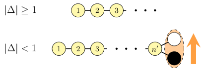
Figure 1: Particle content of the XXZ Heisenberg model for $|\Delta|\geq 1$ (top) and $|\Delta|<1$ (bottom). While the former consist of infinitely many bound magnons with densities $\rho_{a}(u)$, $a\in\mathbb{Z}_{\geq 1}$, the latter reduces to $N_{\rm p}$ particles ($n^{\prime}=N_{\rm p}-2$) whose number depends discontinuously on $\Delta$. Morphology of the graphs reflects how the particles effectively scatter among each other. Black and white end nodes label a distinguished pair which forms a doublet with an effective magnetic moment (orange arrow), being the only particles in the spectrum which transform non-trivially under the spin-reversal operation.

In ergodic dynamical systems, ${\mathcal{D}}^{(q)}=0$ is a consequence of the decay of dynamical correlations in Eq. (2). Integrable systems on the other hand feature stable interacting particles, representing collective thermodynamic excitations which undergo completely elastic (non-diffractive) scattering Zamolodchikov and Zamolodchikov (1979), see Supplemental Material (SM) for further details SM . Such dynamical constraints result in a macroscopic number of conserved quantities ${\hat{\mathcal{Q}}}_{k}$ which prevent generic current-current correlations from completely decaying. This yields Mazur bounds Mazur (1969); Suzuki (1971), ${\mathcal{D}}^{(q)}\geq\frac{1}{2L}\sum_{k}\langle{\hat{\mathcal{J}}}^{(q)}{\hat{\mathcal{Q}}}_{k}\rangle^{2}_{\beta,h}/\langle{\hat{\mathcal{Q}}}^{2}_{k}\rangle_{\beta,h}$, which formally give exact results if all extensive conserved quantities, satisfying $\langle{\hat{\mathcal{Q}}}^{2}_{k}\rangle_{\beta,h}\sim\mathcal{O}(L)$, are included. When ${\hat{\mathcal{J}}}^{(q)}$ belongs to a conserved current, $[{\hat{\mathcal{J}}}^{(q)},\hat{H}]=0$ (e.g. energy current ${\hat{\mathcal{J}}}^{(e)}$ in the Heisenberg model Zotos et al. (1997); Klümper and Sakai (2002)), the Drude weight is trivially finite and reads ${\mathcal{D}}^{(q)}=\lim_{L\to\infty}\tfrac{1}{2L}\langle({\hat{\mathcal{J}}}^{(q)})^{2}\rangle_{\beta,h}$. Conversely, when ${\hat{\mathcal{J}}}^{(q)}$ is not fully conserved, ${\mathcal{D}}^{(q)}>0$ if and only if there exist at least one extensive conserved quantity ${\hat{\mathcal{Q}}}$ with a non-trivial overlap $\langle{\hat{\mathcal{J}}}^{(q)}{\hat{\mathcal{Q}}}\rangle_{\beta,h}>0$.

Spin transport in the XXZ model.–

We proceed by concentrating on the anisotropic Heisenberg model

$$\hat{H}=\sum_{i=1}^{L}\hat{S}^{x}_{i}\hat{S}^{x}_{i+1}+\hat{S}^{y}_{i}\hat{S}^{y}_{i+1}+\Delta(\hat{S}^{z}_{i}\hat{S}^{z}_{i+1}-\tfrac{1}{4}),$$ (4)

in the entire range of anisotropy parameter $\Delta\in\mathbb{R}$. For $|\Delta|>1$ ($|\Delta|\leq 1$) the thermodynamic spectrum is gapped (gapless). We focus here on the elusive case of spin current ${\hat{\mathcal{J}}}^{(s)}$. The presence of chemical potential $h\neq 0$ which couples to $\hat{N}=\sum_{i}\hat{S}^{z}_{i}$ breaks particle-hole symmetry, and renders ${\mathcal{D}}^{(s)}>0$ for all $\Delta\in\mathbb{R}$ by virtue of a non-trivial Mazur bound Zotos et al. (1997). At half filling $h=0$, however, the situation becomes more subtle. Since ${\hat{\mathcal{J}}}^{(s)}$ is odd under the spin-reversal transformation $\hat{R}=\prod_{i}\hat{S}^{x}_{i}$, namely $\hat{R}\,{\hat{\mathcal{J}}}^{(s)}\,\hat{R}=-{\hat{\mathcal{J}}}^{(s)}$, ${\mathcal{D}}^{(s)}$ can only be finite if there exists an extensive conserved quantity ${\hat{\mathcal{Q}}}$ of odd parity and finite overlap $\langle{\hat{\mathcal{J}}}^{(s)}{\hat{\mathcal{Q}}}\rangle_{\beta,h}\neq 0$ Zotos et al. (1997). In spite of substantial numerical evidence, clearly pointing towards ${\mathcal{D}}^{(s)}>0$ for $|\Delta|<1$, the long search for appropriate conservation laws only ended recently with a non-trivial bound obtained in Prosen (2011), followed by a further improved bound derived in Prosen and Ilievski (2013) using a family of odd-parity charges stemming from non-compact representations of the quantized symmetry algebra $\mathcal{U}_{{\mathfrak{q}}}(\mathfrak{sl}_{2})$. Specifically, for commensurate values of anisotropy $\Delta=({\mathfrak{q}}+{\mathfrak{q}}^{-1})/2$, where ${\mathfrak{q}}=\exp{({\rm i}\pi m/\ell)}$ with $m<\ell$ ($\ell>2$) being two co-prime integers, the high-temperature bound (i.e. in the vicinity of $\beta\to 0$) of Prosen and Ilievski (2013) reads explicitly

$${\mathcal{D}}^{(s)}\geq\frac{\beta}{16}\frac{\sin^{2}{(\pi m/\ell)}}{\sin^{2}{(\pi/\ell)}}\left(1-\frac{\ell}{2\pi}\sin{(2\pi/\ell)}\right),$$ (5)

showing an unexpected ‘fractal’ (nowhere-continuous) dependence on the anisotropy parameter $\Delta$. At this stage, a few obvious questions come to mind: (i) is the bound (5) tight, or does it eventually smear out with the inclusion of extra (yet unknown) conservation laws? (ii) What is its value precisely at the isotropic point $\Delta=1$ where the bound (5) becomes trivial? (iii) What is the physical origin of the charges found in Prosen (2011); Prosen and Ilievski (2013). We subsequently provide natural and definite answers to these questions by expressing the Drude weight in terms of balistically propagating particle excitations on the model.

Particle content of the XXZ model.–

Thermodynamic ensembles in integrable models are completely characterized by their particle content Yang and Yang (1969); Takahashi (1971); Gaudin (1971). Local statistical properties are encoded in macrostates, corresponding to a complete set of mode density distributions $\rho_{a}(u)$, where index $a$ labels distinct particle types, and $u$ is the rapidity variable which parametrizes particle momenta $p_{a}(u)$. Distinct types of particles in the spectrum are intimately linked to representation theory of the underlying symmetry group. When $|\Delta|>1$, the thermodynamic spectrum of particles with respect to ferromagnetic vacuum consists of magnons ($a=1$) and bound states thereof ($a\geq 2$) Takahashi (1971); Gaudin (1971). As explained in Ilievski et al. (2016a), these particle species are in a one-to-one correspondence with quantum transfer matrices composed of (auxiliary) finite-dimensional unitary irreducible representations of quantum group $\mathcal{U}_{{\mathfrak{q}}}(\mathfrak{sl}_{2})$, see SM , and also Ilievski et al. (2015a, b, 2016b, 2017). Spin-reversal invariance of macrostates is a simple corollary of unitarity, in turn implying that ${\mathcal{D}}^{(s)}=0$ at $h=0$, in the entire range of anisotropies $|\Delta|\geq 1$. We note that non-unitary highest-weight representations are of infinite dimension and do not enter into the description of magnonic excitations. In the critical regime $|\Delta|<1$ however, one finds an intricate situation where the particle content becomes unstable and changes discontinuously upon varying $\Delta$ Takahashi and Suzuki (1972). When ${\mathfrak{q}}$ is a root of unity, representing a dense set of points in the interval $|\Delta|<1$, the number of independent unitary transfer matrices and magnonic particles both become finite. The latter represent $N_{\rm p}=\sum_{i=1}^{l}\nu_{i}$ bound excitations classified in Takahashi and Suzuki (1972) with aid of continued fraction representation, $m/\ell=1/(\nu_{1}+(1/\nu_{2}+\ldots))\equiv(\nu_{1},\nu_{2},\ldots,\nu_{l})$ (see SM for details SM ), which bijectively correspond to the finite-dimensional irreducible representations of $\mathcal{U}_{{\mathfrak{q}}}(\mathfrak{sl}_{2})$ Ilievski et al. (2016a); Luca et al. (2017). It is shown in Luca et al. (2017) that the densities of a distinguished pair of particles $\rho_{\bullet,\circ}$ (see Fig. 1) map to the spectrum of the odd-parity charges from Prosen and Ilievski (2013); Prosen (2014); Pereira et al. (2014), providing a link to finite-dimensional non-unitary representations of $\mathcal{U}_{{\mathfrak{q}}}(\mathfrak{sl}_{2})$. The lack of unitary implies that $\rho_{\bullet,\circ}(u)$ transform non-trivially under the spin-reversal transformation, meaning that a change in the chemical potential $h$ only explicitly influences macrostates via the distributions $\rho_{\bullet,\circ}(u)$, while other densities get affected indirectly via interparticle interactions. The absence of exceptional particles in the $|\Delta|\geq 1$ regime on the other hand signifies that a macrostate is locally equivalent to its spin-reversed counterpart, and therefore no balistic spin transport between two regions with opposite magnetization density takes place.

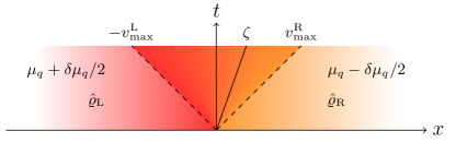
Figure 2: Partitioning protocol: the initial state is prepared in two nearly identical grand canonical equilibria $\hat{\varrho}_{\rm L,R}\propto\exp{(-\beta_{\rm L,R}\hat{H}+h_{\rm L,R}\hat{S}^{z})}$, representing a $q$-charged ($q=s,e$) domain wall of size $\delta q$, with the corresponding chemical potential drop $\delta\mu_{q}=\mu_{q,\rm L}-\mu_{q,\rm R}$ (where $\mu_{e}=\beta$, $\mu_{s}=h$). The initial defect expands in an inhomogeneous state localized within the ‘lightcone’ $v^{\rm L}_{\rm max}<\zeta<v^{\rm R}_{\rm max}$. In the $t\to\infty$ limit, the state along each ray $\zeta=x/t$ relaxes in a quasi-stationary state which is uniquely characterized by particle distributions $\rho_{a}(u,\zeta)$, for $a=1,\ldots,N_{p}$. Drude weight ${\mathcal{D}}^{(q)}$ is proportional to the increment of the total current rate $\lim_{t\to\infty}\mathcal{J}^{(q)}(t;\delta\mu_{q})/t$ in the limit $\delta\mu_{q}\to 0$.

Drude weights from hydrodynamics.–

We now describe a procedure for computing Drude weights using a nonequilibrium ‘partitioning protocol’ developed in Castro-Alvaredo et al. (2016); Bertini et al. (2016), drawing on the earlier ideas of Rubin and Greer (1971); Spohn and Lebowitz (1977) and recent studies of CFTs Bernard and Doyon (2014); Bhaseen et al. (2015); Bernard and Doyon (2016). A simple way to implement a thermodynamic gradient is to consider two partitions representing macroscopically distinct semi-infinite equilibrium states joined together at the point contact, see Fig. 2. The imbalance at the junction induces particle flows between the two subsystems, with a local quasi-stationary state emerging at late times along each ray $\zeta=x/t$. The latter is uniquely specified by the set of distributions $\rho_{a}(u,\zeta)$, pertaining to all types of particles in the spectrum (labelled by $a=1,\ldots,N_{p}$), each obeying a local continuity equation Castro-Alvaredo et al. (2016); Bertini et al. (2016)

$$\partial_{t}\rho_{a}(u,\zeta)+\partial_{x}\left[(v_{a}(u,\zeta)\rho_{a}(u,\zeta)\right]=0.$$ (6)

Notice that, in distinction to non-interacting systems, particles’ velocities $v_{a}(u)$ are dressed due to interactions with a non-trivial background (macrostate) Yang and Yang (1969); Fabian H. L. Essler and Holger Frahm and Frank Göhmann and Andreas Klümper and Vladimir E. Korepin (2005); Quinn and Frolov (2013), $v_{a}(u)=\partial\omega_{a}(u)/\partial p_{a}(u)$, where $\omega_{a}(u)$ and $p_{a}(u)$ are their dressed energy and momenta, respectively (see SM SM ). The solution of Eqs. (6) for each ray $\zeta$ gives a family of densities $\rho_{a}(u,\zeta)$, see Fig. 2.

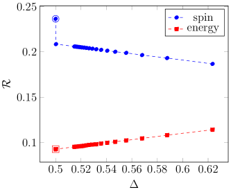
Figure 3: Asymptotic spin (blue) and energy (red) current rates ${\mathcal{R}}^{(q)}=\lim_{t\to\infty}\mathcal{J}^{(q)}(t)/t=\int_{-v^{\rm L}_{\rm max}}^{v^{\rm R}_{\rm max}}{\rm d}\zeta\,j^{(q)}(\zeta;\delta\beta,\delta h)$, emerging by joining two equilibrium states with chemical potentials $h_{\rm L,R}=\pm 1$ and inverse temperatures $\beta_{L,R}=1,3$. Considering the sequence $\Delta=\cos{(\pi/(3+1/\nu_{2}))}$ for $\nu_{2}=2,3,\ldots,20,10^{3}$ (the points at $\nu_{2}=10^{3}$ are obtained by linearly extrapolation of other $\nu_{2}$-points), we demonstrate that $\lim_{\nu_{2}\to\infty}{\mathcal{D}}^{(s)}\neq{\mathcal{D}}^{(s)}(\gamma=\tfrac{\pi}{3})$ (open circle). The same holds in general when approaching a value of $\gamma$ parametrized by $l-1$ integers $\nu_{i}$ as the $\nu_{l}\to\infty$ limit of the order-$l$ sequence of $\nu_{i}$. This indicates that spin current is a nowhere-continuous function of $\Delta$ within $|\Delta|<1$ (cf. Eq. (5) for the exact analytic high-temperature results). Unlike ${\mathcal{R}}^{(s)}$, the thermal current rate ${\mathcal{R}}^{(e)}$ depends continuously on $\Delta$, as shown for $\nu_{1}=3$ (open square).

Computing the Drude weights requires infinitesimal gradients. We thus consider two thermodynamic subsystems prepared in almost identical equilibrium states which differ by a slight amount $\delta q$ in the charge density $q$ and experience a chemical potential jump $\delta\mu_{q}$ at the contact. Transforming (3) to the lightcone frame, we find

$${\mathcal{D}}^{(q)}=\lim_{\delta\mu_{q}\to 0}\frac{\beta}{2\,\delta\mu_{q}}\int_{-v^{\rm L}_{\rm max}}^{v^{\rm R}_{\rm max}}{\rm d}\zeta\,j^{(q)}(\zeta;\delta\mu_{q}),$$ (7)

where $j^{(q)}(\zeta;\delta\mu_{q})$ designates the quasi-stationary expectation value of the current density in the direction of $\zeta$ emanating from the contact. Using the hydrodynamical approach, we first verified the infinite-temperature results of Eq. (5), and found perfect numerical agreement (with absolute precision $<10^{-4}$), at $\Delta=\cos{(\pi m/\ell)}$ for different values of $\nu_{1},\nu_{2},\nu_{3}$. We subsequently confirmed the discontinuous nature of the spin Drude weight as function of $\Delta$ not only at infinite temperature Prosen and Ilievski (2013), but also at finite temperatures $\beta^{-1}$. As temperature is lowered, the discontinuities of ${\mathcal{D}}^{(s)}$ become less pronounced (see Fig. 4), while as $T\to 0$ we find a power-law behavior ${\mathcal{D}}^{(s)}-{\mathcal{D}}^{(s)}(T=0)\sim T^{2/(\ell/m-1)}$ (see Fig. 3 in SM ). Moreover, the hydrodynamic description remains applicable at finite bias $\delta\mu_{q}$, hence allowing to probe quantum transport properties even in the non-linear regime Bertini and Fagotti (2016); Castro-Alvaredo et al. (2016); Bertini et al. (2016); Luca et al. (2017) and revealing that the asymptotic spin-current rate ${\mathcal{R}}^{(s)}=\lim_{t\to\infty}\mathcal{J}^{(s)}(t)/t$ is (unlike e.g. energy current rate ${\mathcal{R}}^{(e)}$) an everywhere discontinuous function of anisotropy $\Delta$, see Fig. 3. Additional figures, showing low-temperature behaviour of ${\mathcal{D}}^{(s)}$ and its dependence on chemical potential $h$, are given in SM SM .

Hubbard model.–

A situation analogous to that of the isotropic Heisenberg model occurs in the (fermionic) Hubbard model Takahashi (1972); Fabian H. L. Essler and Holger Frahm and Frank Göhmann and Andreas Klümper and Vladimir E. Korepin (2005), where in spite of solid evidence in favor of the vanishing finite-temperature spin and charge Drude weights ${\mathcal{D}}^{(c,s)}=0$ in the absence of the respective chemical potentials (see Peres et al. (1999); Kirchner et al. (1999); Carmelo et al. (2013); Karrasch et al. (2014)), the definite conclusion is still lacking Karrasch (2017); Karrasch et al. (2017). A possibility of having additional (unknown) odd-parity conservation laws can however now be quickly ruled out by invoking group-theoretic arguments along the same lines of the isotropic Heinsenberg model. In Hubbard model, the entire space macrostates is in a one-to-one correspondence with particle-hole invariant commuting (fused) transfer matrices, pertaining to a discrete family of unitary irreducible representations of the underlying quantum symmetry Cavaglià et al. (2015). This readily implies vanishing finite-temperature charge/spin Drude weights ${\mathcal{D}}^{(c,s)}=0$ when the corresponding chemical potentials vanish, irrespective of the interaction strength. In the presence of external potentials the Drude weights are known to take finite values by virtue of Mazur bounds, cf. Zotos et al. (1997). As the particle content of Hubbard model is robust against varying the coupling strength, the Drude weights exhibit a continuous dependence on it.

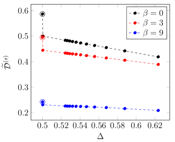
Figure 4: Rescaled spin Drude weight $\widetilde{{\mathcal{D}}}^{(s)}=(16/\beta){\mathcal{D}}^{(s)}$ obtained from Eq. (7) for various temperatures at $\Delta=\cos{(\pi/(3+1/\nu_{2}))}$, for $\nu_{2}=\{2,3,\ldots,12,10^{3}\}$ ($\nu_{2}=10^{3}$ are obtained by linear extrapolation of other $\nu_{2}$-points), and for $\Delta=\cos(\pi/3)=0.5$ (open circles). For a dense set of commensurate anisotropies $\Delta=\cos{(\pi m/\ell)}$, ${\mathcal{D}}^{(s)}$ is found to be a discontinuous function of $\Delta$ at arbitrary finite temperature (see explanation in the caption of Fig. 3).

Conclusions.–

We presented a rigorous and intuitive picture for understanding the phenomenon of ideal conductivity in generic integrable quantum models. Dissipationless transport of generic local charges is shown to be directly linked to the interacting particles of a theory. Nonetheless, spin (or charge) Drude weights in particle-hole symmetric models in the half-filled regimes show exceptional behavior and require a careful analysis by examining the particle content of the model.

While our framework is applicable in general, we focused on the interesting case of the anisotropic Heisenberg model. In the gapped phase, $|\Delta|\geq 1$, particles correspond to an infinite hierarchy of magnonic bound states which are robust under varying the anisotropy parameter Takahashi (1971); Gaudin (1971). The fact that the corresponding particle density operators are insensitive to flipping the spins implies that two thermodynamic states which are characterized terms of mode occupation distributions are (locally) identical, and no ballistic flow of particles across the magnetic domain wall at zero magnetization density can occur. Within the interval $|\Delta|<1$ however, the particle content for commensurate values of $\Delta$ consists of finitely many particles whose number depends discontinuously on $\Delta$ Takahashi and Suzuki (1972). In this case, ballistic spin transport is enabled by the appearance of a distinguished pair of particles which are not invariant under the spin reversal and hence allow for chiral (i.e. spin-carrying) states. It should be stressed that the above qualitative picture can be established independently from any quantitative analysis.

By employing a nonequilibrium partitioning protocol, we presented an exact numerical computation of Drude weights and applied it on the anisotropic Heisenberg spin chain. Our results rigorously prove that the formal infinite-temperature bound derived in Prosen and Ilievski (2013) is the exact Drude weight at infinite temperature, and moreover that the time-asymptotic spin current rate in the XXZ chain is a nowhere-continuous function of $\Delta$ for any finite temperature and even in the non-linear regime. These observations indicate that the physics in the gapless regime $|\Delta|<1$ depends abruptly on the ‘commensurability effect’, resembling the pattern found in famous Hofstadter butterfly Hofstadter (1976); Wiegmann and Zabrodin (1994); Faddeev and Kashaev (1995) multifractal spectrum. As a future task, it would be valuable to perform high-precision finite-time numerical analysis to determine whether the ‘fractality’ can be detected via anomalously large relaxation times.

A number of intriguing open problems remain. Most notably, understanding the microscopic mechanism underlying normal or anomalous diffusion which typically coexists with the ballistic channel, see e.g. Fabricius and McCoy (1998); Sirker et al. (2009); Langer et al. (2009); Žnidarič (2011); Jesenko and Žnidarič (2011)), and recent work Medenjak et al. (2017); Ljubotina et al. (2017). Another open question is to explain diffusive behavior in the semi-classical regime of the Heisenberg ferromagent Prosen and Žunkovič (2013), governed by Landau–Lifshitz action Faddeev and Takhtajan (1987) whose solitons are identified as long-wavelength macroscopic bound states Sutherland (1995).

Note added.

After this work appeared online, an independent work Bulchandani et al. (2017) which partially overlaps with this Letter also shows that the spin Drude weight could be obtained from hydrodynamics.

Acknowledgements.

The authors are grateful to E. Quinn for fruitful discussions and comments on the manuscript, and T. Prosen for valuable feedback. E.I. acknowledges support by VENI grant number 680-47-454 by the Netherlands Organisation for Scientific Research (NWO). J.D.N. acknowledges support by LabEx ENS-ICFP:ANR-10-LABX-0010/ANR-10-IDEX-0001-02 PSL*.

Supplemental Material for
“Microscopic origin of ideal conductivity in integrable quantum models”

This Supplemental Material contains a short review of the particle content in the anisotropic Heisenberg model, along with the description of their dressed energies and momenta, and explicit construction of the corresponding density operators. A few additional figures, showing temperature and chemical potential dependence of the spin Drude weight, are provided as well.

Appendix A Particle content of the anisotropic Heisenberg model

The anisotropic (XXZ) Heisenberg Hamiltonian,

$$\hat{H}=\sum_{i=1}^{L}\hat{S}^{x}_{i}\hat{S}^{x}_{i+1}+\hat{S}^{y}_{i}\hat{S}^{y}_{i+1}+\Delta(\hat{S}^{z}_{i}\hat{S}^{z}_{i+1}-\tfrac{1}{4}),$$ (8)

is diagonalized by Bethe Ansatz. We first assume $|\Delta|>1$ and parametrizing $\Delta=\cosh{(\eta)}$. Any eigenstate in a finite system of size $L$ is assigned a unique set of rapidities $\{u_{k}\}^{M}_{k=1}$ (equiv. a set of quantum numbers), defined from solutions of Bethe equations

$$e^{{\rm i}p(u)L}\prod_{k=1}^{M}S_{11}(u-u_{k})=-1\qquad{\rm for}\quad u\in\{u_{k}\}^{M}_{k=1},$$ (9)

where $M$ is the number of down-turned spins which relates to magnetization $S^{z}=L/2-M$. The (complex) solutions given by $\{u_{k}\}^{M}_{k=1}$ referred to as the Bethe roots. In the thermodynamic limit, defined by taking $L\to\infty$ and $M\to\infty$ limits (keeping ratio $M/L$ finite), the solutions to Bethe equations organize into regular patters which indicate the presence of well-defined particle excitations. Presently, these correspond to magnons and their bound states, known also in the literature as the Bethe strings Takahashi (1971). A ‘$k$-string’ solution reads

$$\{u^{k,m}_{\alpha}\}=\left\{u^{k}_{\alpha}+(k+1-2m)\tfrac{{\rm i}\eta}{2}\right\},\qquad m=1,2,\ldots,k,$$ (10)

where label $\alpha$ enumerates distinct $k$-strings and $m$ runs over their internal rapidities. Scattering amplitudes associated to magnonic particles are

$$S_{j}(u)=\frac{\sin{(u-j\tfrac{{\rm i}\eta}{2})}}{\sin{(u+j\tfrac{{\rm i}\eta}{2})}},\qquad S_{jk}(u)=\prod_{m=-\tfrac{k-1}{2}}^{\tfrac{k-1}{2}}\prod_{n=-\tfrac{j-1}{2}}^{\tfrac{j-1}{2}}S_{2m+2n+2}=S_{|j-k|}S_{j+k}\prod_{m=1}^{{\rm min}(j,k)-1}S^{2}_{|j-k|+2m},$$ (11)

using convention $S_{0}\equiv 0$. In the $L\to\infty$ limit, particle rapidities become densely distributed along the real axis in the rapidity plane. This permits to introduce distributions $\rho_{k}(u)$ of $k$-string particles, along with the dual hole distributions $\bar{\rho}_{k}(u)$ (holes are by definition solutions to Eq. (9) which differ from Bethe roots $u_{k}$). The quantization condition (9) gets accordingly replaced with the integral Bethe–Yang equations Yang and Yang (1969)

$$\rho_{j}+\bar{\rho}_{j}=a_{j}-a_{jk}\star\rho_{k},$$ (12)

where the kernels are given by the derivatives of the scattering phases,

$$a_{j}(u)=\frac{1}{2\pi{\rm i}}\partial_{u}\log S_{j}(u),\qquad a_{jk}(u)=\frac{1}{2\pi{\rm i}}\partial_{u}\log S_{jk}(u).$$ (13)

Here and below we use a compact notation for the convolution integral, $(f\star g)(u)=\int_{\mathbb{R}}f(u-t)g(t){\rm d}v$, and repeated indices are summed over. On each rapidity interval $[u,u+{\rm d}u]$ there is a macroscopic number of microstates, for which a combinatorial entropy density per mode reads Yang and Yang (1969)

$$s_{j}(u)=\rho_{j}\log\left(1+\frac{\bar{\rho}_{j}(u)}{\rho_{j}(u)}\right)+\bar{\rho}_{j}\log\left(1+\frac{\rho_{j}(u)}{\bar{\rho}_{j}(u)}\right).$$ (14)

Isotropic point.

The above results are extended to the isotropic point $\Delta=1$ after taking a scaling limit $u\to u\eta$, and subsequently sending $\eta\to 0$.

A.1 Gapless regime

Classification of particle types in the gapless regime $|\Delta|<1$ can be found in Takahashi and Suzuki (1972). Here, in addition to the magnon type label $k$, an extra parity label $v\in\pm$ is required. Importantly, integers $k$ now no longer coincide with the length of a string, i.e. a number of magnons forming a bound state. Instead, the $k$-th particle consists of $n_{k}$ Bethe roots and carries parity $v_{k}$ (see Takahashi and Suzuki (1972) for further details). Setting $\Delta=\cos{(\gamma)}$, where $\gamma/\pi=m/\ell$ (with $m,\ell$ co-prime integers) is a root of unity, the number of distinct particles in the spectrum is finite. Changing the parametrization $u\to{\rm i}u$, $\eta\to{\rm i}\gamma$ and incorporating the additional parity label, the elementary scattering amplitudes and kernels read

$$S_{k}(u)\to S_{(n_{j},v_{j})}(u)=\frac{\sinh{(u-n_{j}\tfrac{{\rm i}\gamma}{2}+(1-v_{j})\tfrac{{\rm i}\pi}{4})}}{\sinh{(u+n_{j}\tfrac{{\rm i}\gamma}{2}+(1-v_{j})\tfrac{{\rm i}\pi}{4})}},$$ (15)

whereas the full set of scattering kernels are (likewise for the $|\Delta|>1$ case) obtained by fusion (cf. Eqs. (11) and (13)). The Bethe–Yang equations for string get slightly modified, reading

$$\sigma_{j}(\rho_{j}+\bar{\rho}_{j})=a_{j}-a_{jk}\star\rho_{k},$$ (16)

the summation is over all $N_{\rm p}$ types of particles, and $\sigma_{j}={\rm sign}(q_{j})$ depend on $n_{j}$ and $v_{j}$, seeTakahashi and Suzuki (1972).

A.2 Dressing of excitations

Besides the particle content, the hydrodynamic approach requires to extract energies and momenta of individual particles. These are dressed by the interaction with a non-trivial vacuum (a reference macrostate). The dressed energies $\omega_{j}(u)$ and momenta $p_{j}(u)$ of excitations on top of a given macrostate are determined from

$$\omega_{j} =e_{j}+F_{kj}\star\sigma_{k}e_{k}\vartheta_{k},$$ (17)

$$p_{j} =\theta_{j}+F_{kj}\star\sigma_{k}a_{k}\vartheta_{k},$$ (18)

where $e_{j}\simeq a_{j}$ and $\theta_{j}={\rm i}\log S_{j}$ are the bare single particle energy and momenta, respectively, whereas $\vartheta_{k}=\rho_{k}/(\rho_{k}+\bar{\rho}_{k})$ are the filling functions pertaining to the reference macrostate. Shift functions $F_{kj}(u,t)$ encode the $\mathcal{O}(1/L)$ shift of a rapidity $u$ for a particle of type $k$ caused by the injection of a particle of type $j$ carrying rapidity $t$,

$$u\to u-\frac{1}{L}\frac{\sigma_{k}F_{kj}(u,t)}{\rho_{k}(u)+\bar{\rho}_{k}(u)},$$ (19)

and obeys the following integral equation

$$F_{jm}(u,v)=\frac{1}{2\pi{\rm i}}\log S_{jm}(u-v)-\sum_{k=1}^{N_{\rm p}}\int_{\mathbb{R}}{\rm d}t\,\sigma_{k}a_{jk}(u-t)\vartheta_{k}(t)F_{km}(t,v).$$ (20)

A.3 Particle density operators

Every particle in the spectrum is assigned a particle density operator $\hat{\rho}_{j}(u)$, representing (by definition) conserved operators whose action on thermodynamic eigenstates return Bethe root distributions $\rho_{j}(u)$. Particle density operators can thus be perceived as interacting counterparts of the (momentum) mode occupation numbers in non-interacting theories Ilievski et al. (2017).

In the $|\Delta|\geq 1$ regime we put $\Delta=\cosh{(\eta)}=\tfrac{1}{2}({\mathfrak{q}}+{\mathfrak{q}}^{-1})$. The complete set of $\hat{\rho}_{j}(u)$ ($j\in\mathbb{N}$, $u\in\mathbb{R}$) is constructed from commuting fused transfer operators $\hat{T}_{j}(u)$, $[\hat{T}_{j}(u),\hat{T}_{j^{\prime}}(u^{\prime})]=0$, constructed in the standard way,

$$\hat{T}_{j}(u)={\rm Tr}_{\mathcal{V}_{j}}\hat{L}^{(1)}_{j}(u)\hat{L}^{(2)}_{j}(u)\cdots\hat{L}^{(L)}_{j}(u),$$ (21)

where the Lax operators read

$$\hat{L}_{j}(u)=\frac{1}{\sinh{(\eta)}}\begin{pmatrix}\sin{(u+{\rm i}\eta\hat{S}^{z}_{j})}&{\rm i}\sinh{(\eta)}\hat{S}^{-}_{j}\\ {\rm i}\sinh{(\eta)}\hat{S}^{+}_{j}&\sin{(u-{\rm i}\eta\hat{S}^{z}_{j})}\end{pmatrix},$$ (22)

with the ${\mathfrak{q}}$-deformed spin-$j/2$ generators $\hat{S}^{\pm}_{j},\hat{S}^{z}_{j}$ fulfilling the deformed algebraic relations (writing $\hat{K}_{j}={\mathfrak{q}}^{\hat{S}^{z}_{j}}$),

$$\hat{K}_{j}\hat{S}^{\pm}_{j}={\mathfrak{q}}^{\pm 1}\hat{S}^{\pm}_{j}\hat{K}_{j},\quad[\hat{S}^{+}_{j},\hat{S}^{-}_{j}]=\frac{\hat{K}^{2}_{j}-\hat{K}^{-2}_{j}}{{\mathfrak{q}}-{\mathfrak{q}}^{-1}},$$ (23)

acting on (higher-spin) unitary irreducible $(j+1)$-dimensional $\mathcal{U}_{{\mathfrak{q}}}(\mathfrak{sl}_{2})$ modules $\mathcal{V}_{j}$ as

$$\hat{S}^{z}_{j} =(j/2-m)\mathinner{|{m}\rangle}\mathinner{\langle{m}|},$$ (24)

$$\hat{S}^{+}_{j} =\sqrt{[j-m]_{{\mathfrak{q}}}[m+1]_{{\mathfrak{q}}}}\mathinner{|{m+1}\rangle}\mathinner{\langle{m}|},$$ (25)

$$\hat{S}^{-} =\sqrt{[j-m]_{{\mathfrak{q}}}[m+1]_{{\mathfrak{q}}}}\mathinner{|{m}\rangle}\mathinner{\langle{m+1}|},$$ (26)

for $m=0,1,\ldots,j$, and where the ${\mathfrak{q}}$-numbers $[x]_{{\mathfrak{q}}}=({\mathfrak{q}}^{x}-{\mathfrak{q}}^{-x})/({\mathfrak{q}}-{\mathfrak{q}}^{-1})$ have been introduced.

Introducing a set of extensive (local) conserved operators (see Ilievski et al. (2015a, b, 2016a, 2016b)),

$$\hat{X}_{j}(u)=\frac{1}{2\pi{\rm i}}\partial_{u}\log\frac{\hat{T}_{j}(u+\tfrac{{\rm i}\eta}{2})}{T_{0}(u+j\tfrac{{\rm i}\eta}{2})},$$ (27)

defined for spectral parameter $u$ within the ‘physical strip’ $u\in\mathcal{P}$,

$$\mathcal{P}=\left\{u\in\mathbb{C};|{\rm Im}(u)|<\tfrac{\eta}{2}\right\},$$ (28)

the particle density operators $\hat{\rho}_{j}(u)$ ($j\in\mathbb{N}$) are given by Ilievski et al. (2016a)

$$\hat{\rho}_{j}=\hat{X}^{+}_{j}+\hat{X}^{-}_{j}-\hat{X}_{j-1}-\hat{X}_{j+1}\equiv\square\hat{X}_{j},$$ (29)

where $\hat{X}_{0}\equiv 0$ and we have used the compact notation for imaginary shifts, $f^{\pm}(u)\equiv f(u\pm\tfrac{{\rm i}\eta}{2}\mp{\rm i}0)$. Notice that (auxiliary) higher-spin irreducible representations of $\mathcal{U}_{{\mathfrak{q}}}(\mathfrak{sl}_{2})$ (${\mathfrak{q}}\in\mathbb{R}$) are in one-to-one correspondence with the particle types. Moreover, by virtue of unitarity or $\mathcal{V}_{j}$, the particle operators $\hat{\rho}_{j}(u)$ commute with the spin-reversal transformation $\hat{R}=\prod_{i}\hat{S}^{x}_{i}$, $[\hat{R},\hat{\rho}_{j}(u)]=0$.

A.3.1 Interval $|\Delta|<1$.

The critical interval is parametrized by $\Delta=\tfrac{1}{2}({\mathfrak{q}}+{\mathfrak{q}}^{-1})=\cos{(\gamma)}$. For $\gamma/\pi=m/\ell$ being a root of unity, the particle spectrum truncates to a finite set. Writing the (truncated) continued fraction expansion,

$$\frac{\gamma}{\pi}=\frac{1}{\nu_{1}+\frac{1}{\nu_{2}+\frac{1}{\nu_{3}+\ldots}}}\equiv(\nu_{1},\nu_{2},\ldots,\nu_{l}),$$ (30)

the total number of distinct particle types is $N_{\rm p}=\sum_{i=1}^{l}\nu_{i}$. The complete classification can be found in Takahashi and Suzuki (1972), see also Ilievski et al. (2016a). In contrast to the $|\Delta|\geq 1$ case, the number of linearly independent unitary transfer operators $\hat{T}_{j}(u)$ is now finite, with $j=1,2,\ldots,N_{\rm p}-1$. Moreover, labels $j$ do no longer directly correspond to the sizes of auxiliary spins, but are instead non-trivially related to the string lengths and parities (cf. Ilievski et al. (2016a)). The mapping between the particle density operators $\hat{\rho}_{j}(u)$ and a family of (extensive) conserved operators $\hat{X}_{j}(u)$ for arbitrary $\gamma$ has been derived in Ilievski et al. (2016a). Denoting $\hat{\rho}_{N_{\rm p}-1}\equiv\hat{\rho}_{\circ}$ and $\hat{\rho}_{N_{\rm p}}\equiv\hat{\rho}_{\bullet}$, the density operators can be given in a covariant form

$$\hat{\rho}_{j} =\square_{\gamma}\hat{X}_{j},\qquad j=1,2,\ldots N_{\rm p}-2,$$ (31)

$$\hat{\rho}_{\circ}-\hat{\rho}_{\bullet} =\square_{\gamma}\hat{X}_{\ell-1},$$ (32)

with $X_{N_{\rm p}}\equiv 0$, and where $\square_{\gamma}$ is a $\gamma$-dependent discrete wave operator modified introduced in Ilievski et al. (2016a). It is crucial to stress that the spectra of $\hat{X}_{j}(u)$, for $j=1,2,\ldots,N_{\rm p}-1$ only allow to determine the densities for $\rho_{j}(u)$ with $j=1,2,\ldots N_{\rm p}-2$, and the difference of the ‘boundary particles’ $\rho_{\circ}-\rho_{\bullet}$. Therefore, in distinction to $|\Delta|\geq 1$, the particle content in the interval $|\Delta|<1$ (at ${\mathfrak{q}}$ root of unity) is no longer in bijection with unitary (i.e. spin-reversal invariant) irreducible representations of the corresponding quantum symmetry $\mathcal{U}_{{\mathfrak{q}}}(\mathfrak{sl}_{2})$. In order retrieve the missing information and obtain $\hat{\rho}_{\circ}$ and $\hat{\rho}_{\bullet}$ separately, the set $\hat{X}_{j}(u)$ has to be supplemented with an extra conserved operator $\hat{Z}(u)$ (cf. Eq. (36) below) built from non-unitary auxiliary irreducible representations of $\mathcal{U}_{{\mathfrak{q}}}(\mathfrak{sl}_{2})$ (with ${\mathfrak{q}}$ being a root of unity), constructed first in Prosen (2011); Prosen and Ilievski (2013) (see also Prosen (2014); Pereira et al. (2014)). The distinguished property of $\hat{Z}(u)$ is that it flips the sign under spin-reversal transformation, $\hat{R}\hat{Z}(u)\hat{R}=-\hat{Z}(u)$.

For instance, in the simplest case of $\gamma/\pi=1/\nu_{1}=1/\ell$, the lengths and parties of particles are

$$n_{j} =j,\quad v_{j}=1,\qquad j=1,2,\ldots,\nu_{1}-1,$$ (33)

$$n_{\nu_{1}} =1,\quad v_{\nu_{1}}=-1.$$ (34)

Here $\square_{\gamma}$ coincides with the gapped counterpart $\square$, with the imaginary shifts given now by ${\rm i}\gamma/2$. At the boundary nodes we have Luca et al. (2017)

$$\hat{\rho}_{\bullet}=-\frac{1}{2}\left(\hat{X}^{+}_{\ell-1}+\hat{X}^{-}_{\ell-1}\right)-\frac{1}{2\gamma}\int_{-\gamma/2}^{\gamma/2}{\rm d}z\,\hat{X}^{\prime}(u+{\rm i}z),$$ (35)

where

$$\hat{X}^{\prime}(u)=\partial_{\alpha}\hat{X}_{\ell-1,\alpha}(u)|_{\alpha=0}=\hat{Z}(u)-\frac{\gamma}{2\pi\cosh^{2}{(u)}}.$$ (36)

Here $\hat{X}_{\ell-1,\alpha}(u)$ is defined as a conserved operator built from the (finite-dimensional) non-unitary irreducible representation $\mathcal{V}_{\ell-1,\alpha}$, with the action of ${\mathfrak{q}}$-deformed spin operators reading Luca et al. (2017)

$$\hat{K}_{\ell-1,\alpha}\mathinner{|{m}\rangle} ={\mathfrak{q}}^{m+\alpha}\mathinner{|{m}\rangle},$$ (37)

$$\hat{S}^{+}_{\ell-1,\alpha}\mathinner{|{m}\rangle} =-[m-\ell+1+2\alpha]_{{\mathfrak{q}}}\mathinner{|{m+1}\rangle},$$ (38)

$$\hat{S}^{-}_{\ell-1,\alpha}\mathinner{|{m}\rangle} =[m+\ell-1]_{{\mathfrak{q}}}\mathinner{|{m-1}\rangle},$$ (39)

where $m=-\tfrac{1}{2}(\ell-1),\ldots,\tfrac{1}{2}(\ell-1)$. The upshot of this is that macrostates for which $\rho_{\circ}(u)\neq\bar{\rho}_{\bullet}(u)$ carry non-vanishing amount of $Z$-charge, implying that the spin reversal operation yields a (locally) distinguishable macrostate (i.e. a state with distinct particle densities). In the context of our application, this enables a ballistic drift of particles across a magnetic domain wall.

Appendix B Additional plots

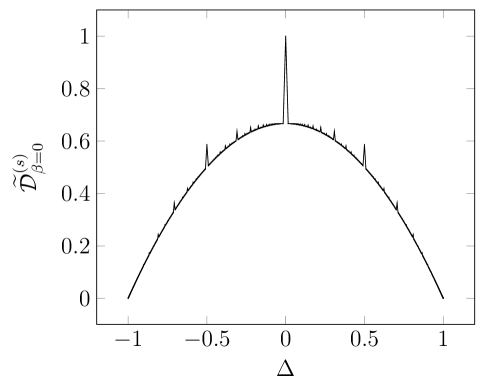
Figure 5: Rescaled spin Drude weight $\widetilde{{\mathcal{D}}}^{(s)}=(16/\beta){\mathcal{D}}^{(s)}$ in the high-temperature $\beta\to 0$ limit as function of anisotropy $\Delta$, given by analytic expression, equation (5) in the main text. The result was obtained in Prosen and Ilievski (2013) as a lower bound for the spin Drude weight. In the Letter we rigorously prove that the bound is optimal and coincides with the exact value of ${\mathcal{D}}^{(s)}$ at infinite temperature.

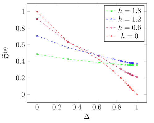
Figure 6: Rescaled spin Drude weight $\widetilde{{\mathcal{D}}}^{(s)}=(16/\beta){\mathcal{D}}^{(s)}$ at $\beta\to 0$ as function of anisotropy $\Delta$ for $\Delta=0$ and $\Delta=\cos{(\frac{\pi}{\nu_{1}+1/2})}$ with $\nu_{1}=\{2,3,\ldots,12\}$ and $\nu_{2}\to\infty$ (obtained from the previous $\nu_{2}$-points by linear fitting), shown for various chemical potentials $\mu_{s}=h$.

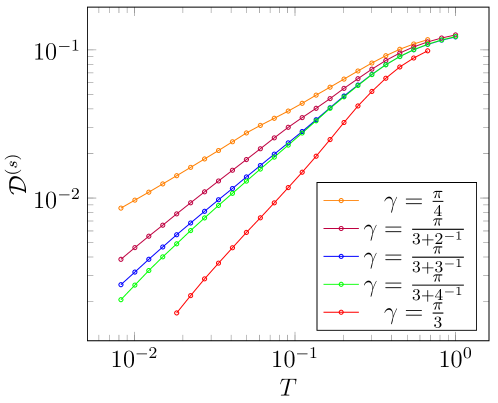
Figure 7: Log-log scale: Spin Drude weight ${\mathcal{D}}^{(s)}-{\mathcal{D}}^{(s)}(T=0)$ as function of temperature $T=\beta^{-1}$ at $\Delta=\cos{(\gamma)}$. For $\gamma=\pi/\nu_{1}$ we confirm the scaling ${\mathcal{D}}^{(s)}-{\mathcal{D}}^{(s)}(T=0)\sim T^{2/(\nu_{1}-1)}$ found earlier in Zotos (1999), while at $\gamma/\pi=1/(\nu_{1}+1/(\nu_{2}+1/\nu_{3}))$ we observe the power law ${\mathcal{D}}^{(s)}-{\mathcal{D}}^{(s)}(T=0)\sim T^{2/(\gamma/\pi-1)}$.

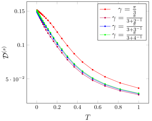
Figure 8: Spin Drude weight ${\mathcal{D}}^{(s)}$ as function of temperature $T=\beta^{-1}$, shown for $\Delta=\cos{(\gamma)}$ at $\gamma/\pi=1/(3+1/\nu_{2})$ for $\nu_{2}=\{2,3,4,\ldots\}$. While in the low-$T$ regime ${\mathcal{D}}^{(s)}$ for $\Delta=\cos{(\pi/(3+4^{-1}))}\approx 0.568$ and $\Delta=0.5$ are comparable to each other, they significantly differ at higher temperatures.

References

- Castella et al. (1995) H. Castella, X. Zotos, and P. Prelovšek, Physical Review Letters 74, 972 (1995).
- Zotos et al. (1997) X. Zotos, F. Naef, and P. Prelovšek, Physical Review B 55, 11029 (1997).
- Sologubenko et al. (2001) A. V. Sologubenko, K. Giannò, H. R. Ott, A. Vietkine, and A. Revcolevschi, 64 (2001), 10.1103/physrevb.64.054412.
- Hess et al. (2001) C. Hess, C. Baumann, U. Ammerahl, B. Büchner, F. Heidrich-Meisner, W. Brenig, and A. Revcolevschi, Physical Review B 64 (2001), 10.1103/physrevb.64.184305.
- Hlubek et al. (2010) N. Hlubek, P. Ribeiro, R. Saint-Martin, A. Revcolevschi, G. Roth, G. Behr, B. Büchner, and C. Hess, 81 (2010), 10.1103/physrevb.81.020405.
- Maeter et al. (2013) H. Maeter, A. A. Zvyagin, H. Luetkens, G. Pascua, Z. Shermadini, R. Saint-Martin, A. Revcolevschi, C. Hess, B. Büchner, and H.-H. Klauss, Journal of Physics: Condensed Matter 25, 365601 (2013).
- Hild et al. (2014) S. Hild, T. Fukuhara, P. Schauß, J. Zeiher, M. Knap, E. Demler, I. Bloch, and C. Gross, Physical Review Letters 113 (2014), 10.1103/physrevlett.113.147205.
- Carmelo et al. (2015) J. M. P. Carmelo, T. Prosen, and D. K. Campbell, Physical Review B 92 (2015), 10.1103/physrevb.92.165133.
- Karrasch (2017) C. Karrasch, New Journal of Physics 19, 033027 (2017).
- Carmelo and Prosen (2017) J. Carmelo and T. Prosen, Nuclear Physics B 914, 62 (2017).
- Peres et al. (1999) N. M. R. Peres, P. D. Sacramento, D. K. Campbell, and J. M. P. Carmelo, Physical Review B 59, 7382 (1999).
- Zotos (1999) X. Zotos, Physical Review Letters 82, 1764 (1999).
- Sirker et al. (2011) J. Sirker, R. G. Pereira, and I. Affleck, Physical Review B 83 (2011), 10.1103/physrevb.83.035115.
- Herbrych et al. (2011) J. Herbrych, P. Prelovšek, and X. Zotos, Physical Review B 84 (2011), 10.1103/physrevb.84.155125.
- Žnidarič (2011) M. Žnidarič, Physical Review Letters 106 (2011), 10.1103/physrevlett.106.220601.
- Narozhny et al. (1998) B. N. Narozhny, A. J. Millis, and N. Andrei, Physical Review B 58, R2921 (1998).
- Alvarez and Gros (2002) J. V. Alvarez and C. Gros, Physical Review Letters 88 (2002), 10.1103/physrevlett.88.077203.
- Heidrich-Meisner et al. (2003) F. Heidrich-Meisner, A. Honecker, D. C. Cabra, and W. Brenig, Physical Review B 68 (2003), 10.1103/physrevb.68.189901.
- Fujimoto and Kawakami (2003) S. Fujimoto and N. Kawakami, Physical Review Letters 90 (2003), 10.1103/physrevlett.90.197202.
- Benz et al. (2005) J. Benz, T. Fukui, A. Klümper, and C. Scheeren, Journal of the Physical Society of Japan 74, 181 (2005).
- Karrasch et al. (2012) C. Karrasch, J. H. Bardarson, and J. E. Moore, Physical Review Letters 108 (2012), 10.1103/physrevlett.108.227206.
- Steinigeweg et al. (2014) R. Steinigeweg, J. Gemmer, and W. Brenig, Physical Review Letters 112 (2014), 10.1103/physrevlett.112.120601.
- Castro-Alvaredo et al. (2016) O. A. Castro-Alvaredo, B. Doyon, and T. Yoshimura, Physical Review X 6 (2016), 10.1103/physrevx.6.041065.
- Bertini et al. (2016) B. Bertini, M. Collura, J. D. Nardis, and M. Fagotti, Physical Review Letters 117 (2016), 10.1103/physrevlett.117.207201.
- Kubo (1957) R. Kubo, Journal of the Physical Society of Japan 12, 570 (1957).
- Mahan (2000) G. D. Mahan, Many-Particle Physics (Springer Nature, 2000).
- Note (1) While the restriction to grand canonical ensembles adopted in this work is suitable for studying (spin,energy) transport, our framework permits to consider completely general equilibrium states in a system.
- Karrasch et al. (2013) C. Karrasch, J. H. Bardarson, and J. E. Moore, New Journal of Physics 15, 083031 (2013).
- Karrasch et al. (2014) C. Karrasch, D. M. Kennes, and J. E. Moore, Physical Review B 90 (2014), 10.1103/physrevb.90.155104.
- Vasseur et al. (2015) R. Vasseur, C. Karrasch, and J. E. Moore, Physical Review Letters 115 (2015), 10.1103/PhysRevLett.115.267201.
- Kohn (1964) W. Kohn, Physical Review 133, A171 (1964).
- Shastry and Sutherland (1990) B. S. Shastry and B. Sutherland, Physical Review Letters 65, 243 (1990).
- Fujimoto and Kawakami (1998) S. Fujimoto and N. Kawakami, Journal of Physics A: Mathematical and General 31, 465 (1998).
- Fujimoto (1999) S. Fujimoto, Journal of the Physical Society of Japan 68, 2810 (1999).
- Ilievski and Prosen (2012) E. Ilievski and T. Prosen, Communications in Mathematical Physics 318, 809 (2012).
- Zamolodchikov and Zamolodchikov (1979) A. B. Zamolodchikov and A. B. Zamolodchikov, Annals of physics 120, 253 (1979).
- (37) Supplemental Material associated with this manuscript.
- Mazur (1969) P. Mazur, Physica 43, 533 (1969).
- Suzuki (1971) M. Suzuki, Physica 51, 277 (1971).
- Klümper and Sakai (2002) A. Klümper and K. Sakai, Journal of Physics A: Mathematical and General 35, 2173 (2002).
- Prosen (2011) T. Prosen, Physical Review Letters 106 (2011), 10.1103/physrevlett.106.217206.
- Prosen and Ilievski (2013) T. Prosen and E. Ilievski, Physical Review Letters 111 (2013), 10.1103/physrevlett.111.057203.
- Yang and Yang (1969) C.-N. Yang and C. Yang, Journal of Mathematical Physics 10, 1115 (1969).
- Takahashi (1971) M. Takahashi, Progress of Theoretical Physics 46, 401 (1971).
- Gaudin (1971) M. Gaudin, Physical Review Letters 26, 1301 (1971).
- Ilievski et al. (2016a) E. Ilievski, E. Quinn, J. De Nardis, and M. Brockmann, Journal of Statistical Mechanics: Theory and Experiment 2016, 063101 (2016a).
- Ilievski et al. (2015a) E. Ilievski, M. Medenjak, and T. Prosen, Physical Review Letters 115, 120601 (2015a).
- Ilievski et al. (2015b) E. Ilievski, J. De Nardis, B. Wouters, J.-S. Caux, F. H. Essler, and T. Prosen, Physical Review Letters 115, 157201 (2015b).
- Ilievski et al. (2016b) E. Ilievski, M. Medenjak, T. Prosen, and L. Zadnik, J. Stat. Mech. 2016, 064008 (2016b).
- Ilievski et al. (2017) E. Ilievski, E. Quinn, and J.-S. Caux, Physical Review B 95 (2017), 10.1103/physrevb.95.115128.
- Takahashi and Suzuki (1972) M. Takahashi and M. Suzuki, Progress of theoretical physics 48, 2187 (1972).
- Luca et al. (2017) A. D. Luca, M. Collura, and J. D. Nardis, Physical Review B 96 (2017), 10.1103/physrevb.96.020403.
- Prosen (2014) T. Prosen, Nuclear Physics B 886, 1177 (2014).
- Pereira et al. (2014) R. G. Pereira, V. Pasquier, J. Sirker, and I. Affleck, Journal of Statistical Mechanics: Theory and Experiment 2014, P09037 (2014).
- Rubin and Greer (1971) R. J. Rubin and W. L. Greer, Journal of Mathematical Physics 12, 1686 (1971).
- Spohn and Lebowitz (1977) H. Spohn and J. L. Lebowitz, Communications in Mathematical Physics 54, 97 (1977).
- Bernard and Doyon (2014) D. Bernard and B. Doyon, Annales Henri Poincaré 16, 113 (2014).
- Bhaseen et al. (2015) M. J. Bhaseen, B. Doyon, A. Lucas, and K. Schalm, Nature Physics 11, 509 (2015).
- Bernard and Doyon (2016) D. Bernard and B. Doyon, J. Stat. Mech. 2016, 064005 (2016).
- Fabian H. L. Essler and Holger Frahm and Frank Göhmann and Andreas Klümper and Vladimir E. Korepin (2005) Fabian H. L. Essler and Holger Frahm and Frank Göhmann and Andreas Klümper and Vladimir E. Korepin, The One-Dimensional Hubbard Model (Cambridge University Press (CUP), 2005).
- Quinn and Frolov (2013) E. Quinn and S. Frolov, Journal of Physics A: Mathematical and Theoretical 46, 205001 (2013).
- Bertini and Fagotti (2016) B. Bertini and M. Fagotti, Physical Review Letters 117 (2016), 10.1103/physrevlett.117.130402.
- Takahashi (1972) M. Takahashi, Progress of Theoretical Physics 47, 69 (1972).
- Kirchner et al. (1999) S. Kirchner, H. G. Evertz, and W. Hanke, 59, 1825 (1999).
- Carmelo et al. (2013) J. Carmelo, S.-J. Gu, and P. Sacramento, Annals of Physics 339, 484 (2013).
- Karrasch et al. (2017) C. Karrasch, T. Prosen, and F. Heidrich-Meisner, Physical Review B 95 (2017), 10.1103/physrevb.95.060406.
- Cavaglià et al. (2015) A. Cavaglià, M. Cornagliotto, M. Mattelliano, and R. Tateo, Journal of High Energy Physics 2015 (2015), 10.1007/jhep06(2015)015.
- Hofstadter (1976) D. R. Hofstadter, Physical Review B 14, 2239 (1976).
- Wiegmann and Zabrodin (1994) P. Wiegmann and A. Zabrodin, Nuclear Physics B 422, 495 (1994).
- Faddeev and Kashaev (1995) L. D. Faddeev and R. M. Kashaev, Communications in Mathematical Physics 169, 181 (1995).
- Fabricius and McCoy (1998) K. Fabricius and B. M. McCoy, Physical Review B 57, 8340 (1998).
- Sirker et al. (2009) J. Sirker, R. G. Pereira, and I. Affleck, Physical Review Letters 103 (2009), 10.1103/physrevlett.103.216602.
- Langer et al. (2009) S. Langer, F. Heidrich-Meisner, J. Gemmer, I. P. McCulloch, and U. Schollwöck, Physical Review B 79 (2009), 10.1103/physrevb.79.214409.
- Jesenko and Žnidarič (2011) S. Jesenko and M. Žnidarič, Physical Review B 84 (2011), 10.1103/physrevb.84.174438.
- Medenjak et al. (2017) M. Medenjak, C. Karrasch, and T. Prosen, arXiv preprint arXiv:1702.04677 (2017).
- Ljubotina et al. (2017) M. Ljubotina, M. Žnidarič, and T. Prosen, Nature Communications 8, 16117 (2017).
- Prosen and Žunkovič (2013) T. Prosen and B. Žunkovič, Physical Review Letters 111 (2013), 10.1103/physrevlett.111.040602.
- Faddeev and Takhtajan (1987) L. D. Faddeev and L. A. Takhtajan, Hamiltonian Methods in the Theory of Solitons (Springer Nature, 1987).
- Sutherland (1995) B. Sutherland, Physical Review Letters 74, 816 (1995).
- Bulchandani et al. (2017) V. B. Bulchandani, R. Vasseur, C. Karrasch, and J. E. Moore, arXiv preprint arXiv:1702.06146 (2017).