Topological first-order vortices in a gauged $CP\left(2\right)$ model

Abstract

We study time-independent radially symmetric first-order solitons in a $CP(2)$ model interacting with an Abelian gauge field whose dynamics is controlled by the usual Maxwell term. In this sense, we develop a consistent first-order framework verifying the existence of a well-defined lower bound for the corresponding energy. We saturate such a lower bound by focusing on those solutions satisfying a particular set of coupled first-order differential equations. We solve these equations numerically using appropriate boundary conditions giving rise to regular structures possessing finite-energy. We also comment the main features these configurations exhibit. Moreover, we highlight that, despite the different solutions we consider for an auxiliary function $\beta\left(r\right)$ labeling the model (therefore splitting our investigation in two a priori distinct branches), all resulting scenarios engender the very same phenomenology, being physically equivalent.

I Introduction

Topological objects are frequently described as the time-independent regular solutions possessing finite-energy arising from highly nonlinear Euler-Lagrange equations in the presence of appropriated boundary conditions n5 . In some particular cases, the Bogomol’nyi-Prasad-Sommerfield (BPS) formalism allows to show that these solutions can also satisfy a set of coupled first-order differential equations, the BPS ones n4 .

In this sense, vortices are radially symmetric solitonic configurations appearing in a planar scalar scenario endowed by a gauge field, their energies being commonly proportional to the magnetic flux, both ones being quantized, i.e. proportional to an integer winding number. In the context of the classical field theory, these structures were firstly studied within the Maxwell-Higgs system, the self-interacting potential possessing no symmetric vacuum engendering topological first-order vortex solutions only n1 . Similar objects were also encountered in a Chern-Simons-Higgs scenario, the corresponding theory giving rise to both topological and nontopological first-order vortices cshv .

Furthermore, during the last years, many additional progress have been made regarding first-order vortices arising within different theoretical scenarios, including generalizations of the Abelian-Higgs theories gaht , Lorentz-violating systems lvs and gauged models with noncanonical kinetic terms gmnckt , many of them being applied as an attempt to explain different cosmological and gravitational phenomena ames .

In particular, in view of the developments introduced in cp1 , the question on whether a gauged $CP(N-1)$ model with $N>2$ supports topological vortices arises in a rather natural way, mainly due to the straight relation between the $CP(N-1)$ theory and the four-dimensional Yang-Mills-Higgs one, the first mapping some interesting properties of the second cpn-1 .

In a very recent contribution loginov , the author have investigated topological vortices arising within a gauged $CP(N-1)$ model, the electromagnetic and the $CP(N-1)$ scalar fields interacting minimally, the dynamics of the gauge sector being controlled by the usual Maxwell term. In that work, the author have considered only non-BPS profiles, the corresponding solutions being obtained via the second-order Euler-Lagrange equations, from which the author have also studied interesting properties of the resulting structures, such as the way the energy and magnetic flux depend on the parameters of the overall model.

We now go a little bit further into such theme by considering the very same theoretical scenario, but now looking for a general first-order framework engendering radially symmetric vortices, whilst studying how these structures differ from their non-BPS counterparts.

In order to present our results, this manuscript is organized as follows: firstly, in the next Section II, we introduce the gauged $CP(N-1)$ model we study, presenting some basic definitions and conventions. We particularize our investigation by focusing on the time-independent fields giving rise to radially symmetric configurations. In such a scenario, we look for a consistent first-order framework by manipulating the expression for the effective energy functional in order to establish a well-defined lower bound for the corresponding total energy (here, it is important to point out that such construction is only possible when a particular constraint involving the potential is fulfilled). We verify that this bound is saturated (the energy being minimized) when the profile functions describing the original fields satisfy a particular set of coupled first-order equations. We also calculate general results for the energy bound and the magnetic flux inherent to the BPS configurations. In the Section III, we investigate in detail the way the first-order expressions introduced previously generate legitimate solutions, whilst using the aforecited constraint to determine the potential term defining the vacuum manifold of the corresponding model. Then, we solve the first-order equations numerically via convenient boundary conditions, from which we obtain regular configurations possessing finite energy, also identifying and commenting the main features these solitons engender. Finally, in the Sec. IV, we present our conclusions and general perspectives regarding future contributions.

We highlight that, throughout all this manuscript, we use the natural units system together with $\eta^{\mu\nu}=\left(+--\right)$ for the planar metric signature.

II The overall model

We begin our investigation by considering the planar gauged $CP(N-1)$ model introduced in loginov , its Lagrange density reading

$$\mathcal{L}=-\frac{1}{4}F_{\mu\nu}F^{\mu\nu}+\left(P_{ab}D_{\mu}\phi_{b}\right)^{\ast}P_{ac}D^{\mu}\phi_{c}-V\left(\left|\phi\right|\right)\text{,}$$ (1)

with $F_{\mu\nu}=\partial_{\mu}A_{\nu}-\partial_{\nu}A_{\mu}$ being the usual electromagnetic field strength tensor, $P_{ab}=\delta_{ab}-h^{-1}\phi_{a}\phi_{b}^{\ast}$ standing for a projection operator defined conveniently and $D_{\mu}\phi_{a}=\partial_{\mu}\phi_{a}-igA_{\mu}Q_{ab}\phi_{b}$ representing the corresponding covariant derivative (here, $Q_{ab}$ is a charge matrix, diagonal and real). Additionally, the $CP(N-1)$ field $\phi$ is constrained to satisfy $\phi_{a}^{\ast}\phi_{a}=h$. In our notation, Greek indexes run over time-space coordinates, the Latin ones counting the complex components of the $CP(N-1)$ field themselves.

It is instructive to write down the static Gauss law coming from (1), i.e. (here, $j$ runs over spatial coordinates only)

$$\partial_{j}\partial^{j}A^{0}=J^{0}\text{,}$$ (2)

the charge density being

$$J^{0}=ig\left[\left(P_{ab}D^{0}\phi_{b}\right)^{\ast}P_{ac}Q_{cd}\phi_{d}-P_{ab}D^{0}\phi_{b}\left(P_{ac}Q_{cd}\phi_{d}\right)^{\ast}\right]\text{,}$$ (3)

where $D^{0}\phi_{b}=-igQ_{bc}\phi_{c}A^{0}$. In this sense, according the Gauss law (2), one concludes that the static configurations that the model (1) engenders have null electric charge, being then compatible with the gauge condition $A^{0}=0$ which satisfies (2) identically.

In this work, for the sake of simplicity, we consider the $N=3$ case, this way reducing our study to the $CP(2)$ scenario. In such a context, we look for time-independent solutions with radial symmetry. In this sense, we guide our calculations using the standard map (with winding numbers $m_{1}$, $m_{2}$ and $m_{3}\in\mathbb{Z}$)

$$A_{i}=-\frac{1}{gr}\epsilon^{ij}n^{j}A\left(r\right)\text{,}$$ (4)

$$\left(\begin{array}[]{c}\phi_{1}\\ \phi_{2}\\ \phi_{3}\end{array}\right)=h^{\frac{1}{2}}\left(\begin{array}[]{c}e^{im_{1}\theta}\sin\left(\alpha\left(r\right)\right)\cos\left(\beta\left(r\right)\right)\\ e^{im_{2}\theta}\sin\left(\alpha\left(r\right)\right)\sin\left(\beta\left(r\right)\right)\\ e^{im_{3}\theta}\cos\left(\alpha\left(r\right)\right)\end{array}\right)\text{,}$$ (5)

with $\epsilon^{ij}$ and $n^{j}=\left(\cos\theta,\sin\theta\right)$ being the bidimensional Levi-Civita tensor ($\epsilon^{12}=+1$) and the position unit vector, respectively, the magnetic field being expressed as

$$B\left(r\right)=-\frac{1}{gr}\frac{dA}{dr}\text{.}$$ (6)

It is worthwhile to note that, once we are interested in regular solutions presenting no divergences, the profile functions $\alpha\left(r\right)$ and $A\left(r\right)$ must obey

$$\alpha(r\rightarrow 0)\rightarrow 0\text{ \ \ and \ \ }A(r\rightarrow 0)\rightarrow 0\text{.}$$ (7)

As we demonstrate below, we use these conditions to obtain well-behaved field solutions related to (1).

We highlight that, regarding the combination between the charge matrix $Q_{ab}$ and the winding numbers in (5), there are two possibilities engendering topological solitons: (i) $Q=\lambda_{3}/2$ and $m_{1}=-m_{2}=m$, and (ii) $Q=\lambda_{8}/2$ and $m_{1}=m_{2}=m$ (both ones with $m_{3}=0$, $\lambda_{3}$ and $\lambda_{8}$ being the diagonal Gell-Mann matrices, i.e. $\lambda_{3}=$diag$\left(1,-1,0\right)$ and $\sqrt{3}\lambda_{8}=$diag$\left(1,1,-2\right)$). Nevertheless, in loginov , the author have demonstrated that these two combinations simply mimic each other, this way existing only one effective scenario. Therefore, in this work, we investigate only the case defined by $m_{1}=-m_{2}=m$, $m_{3}=0$ and

$$Q_{ab}=\frac{1}{2}\lambda_{3}=\frac{1}{2}\text{diag}\left(1,-1,0\right)\text{,}$$ (8)

for convenience.

The differential equation for the profile function $\beta\left(r\right)$ reads

$$\frac{d^{2}\beta}{dr^{2}}+\left(\frac{1}{r}+2\frac{d\alpha}{dr}\cot\alpha\right)\frac{d\beta}{dr}=\frac{\sin^{2}\alpha\sin\left(4\beta\right)}{r^{2}}\left(m-\frac{A}{2}\right)^{2}\text{,}$$ (9)

giving rise to two constant solutions, i.e.

$$\beta\left(r\right)=\beta_{1}=\frac{\pi}{4}+\frac{\pi}{2}k\text{ \ \ or \ \ }\beta\left(r\right)=\beta_{2}=\frac{\pi}{2}k\text{,}$$ (10)

with $k\in\mathbb{Z}$. A priori, these solutions define two different cases. However, as we demonstrate later below, these cases engender the very same phenomenology, at least when concerning the first-order results at the classical level.

It is important to say that, from this point on, our expressions effectively describe the scenario defined by the choices we have introduced above.

We focus our attention on those solutions satisfying a particular set of coupled first-order equations. In this work, we obtain these equations by following the canonical approach, i.e. by requiring the minimization of the total energy of the system, the starting-point being the expression for the energy-momentum tensor related to the model (1), i.e.

$$\mathcal{T}_{\lambda\rho}=-F_{\lambda\mu}F_{\rho}{}^{\mu}+2\left(P_{ab}D_{\lambda}\phi_{b}\right)^{\ast}P_{ac}D_{\rho}\phi_{c}-\eta_{\lambda\rho}\mathcal{L}\text{,}$$ (11)

from which one gets the radially symmetric energy density ($\varepsilon\equiv\mathcal{T}_{00}=-\mathcal{L}$)

$$\varepsilon=\frac{B^{2}}{2}+h\left[\left(\frac{d\alpha}{dr}\right)^{2}+\frac{W}{r^{2}}\left(\frac{A}{2}-m\right)^{2}\sin^{2}\alpha\right]+V\text{,}$$ (12)

the corresponding total energy reading

$$\frac{E}{2\pi} = \int\left(\frac{B^{2}}{2}+V\right)rdr$$

$$+h\int\left[\left(\frac{d\alpha}{dr}\right)^{2}+\frac{W}{r^{2}}\left(\frac{A}{2}-m\right)^{2}\sin^{2}\alpha\right]rdr\text{,}$$

where we have introduced the auxiliary function

$$W=W\left(\alpha,\beta\right)=1-\sin^{2}\alpha\cos^{2}\left(2\beta\right)\text{,}$$ (14)

the solution for $\beta\left(r\right)$ being necessarily one of those stated in (10).

In order to find the correspondent first-order equations, we write the expression (II) in the convenient form

$$\frac{E}{2\pi}=\frac{1}{2}\int\left(B\mp\sqrt{2V}\right)^{2}rdr$$ (15)

$$+h\int\left[\frac{d\alpha}{dr}\mp\frac{\sqrt{W}}{r}\left(\frac{A}{2}-m\right)\sin\alpha\right]^{2}rdr$$

$$\mp\int\left[\frac{d\left(A-2m\right)}{dr}\frac{\sqrt{2V}}{g}+\left(A-2m\right)h\sqrt{W}\frac{d\left(\cos\alpha\right)}{dr}\right]dr\text{.}$$

The expression in the third row above can be converted in a total derivative whether we consider the fundamental constraint

$$\frac{1}{g}\frac{d}{dr}\left(\sqrt{2V}\right)=h\sqrt{W}\frac{d\left(\cos\alpha\right)}{dr}\text{.}$$ (16)

This way, the energy (15) can be rewritten as

$$E=E_{bps}+\pi\int\left(B\mp\sqrt{2V}\right)^{2}rdr$$ (17)

$$\text{ \ \ \ \ \ }+2\pi h\int\left[\frac{d\alpha}{dr}\mp\frac{\sqrt{W}}{r}\left(\frac{A}{2}-m\right)\sin\alpha\right]^{2}rdr\text{,}$$

where we have defined $E_{bps}$ as

$$E_{bps}=2\pi\int r\varepsilon_{bps}dr\text{,}$$ (18)

with $\varepsilon_{bps}$ being given by

$$\varepsilon_{bps}=\mp\frac{1}{gr}\frac{d}{dr}\left[\left(A-2m\right)\sqrt{2V}\right]\text{.}$$ (19)

The quantity $E_{bps}$ is finite and positive when the potential fulfills $V(r\rightarrow\infty)=0$, with $V_{0}\equiv V\left(r\rightarrow 0\right)$ being finite and positive also.

Equation (17) shows that the corresponding energy exhibits a well-defined lower bound (a property inherent to such a first-order construction), this bound being saturated when the profile functions $\alpha\left(r\right)$ and $A\left(r\right)$ obey

$$B=\pm\sqrt{2V}\text{,}$$ (20)

$$\frac{d\alpha}{dr}=\pm\frac{\sin\alpha}{r}\left(\frac{A}{2}-m\right)\sqrt{1-\sin^{2}\alpha\cos^{2}\left(2\beta\right)}\text{,}$$ (21)

which are the effective first-order equations the model (1) engenders. In this sense, when (20) and (21) are satisfied, the total energy of the resulting configurations can be evaluated directly, reading (the upper (lower) sign holding for negative (positive) values of $m$)

$$E=E_{bps}=\mp\frac{4\pi}{g}m\sqrt{2V_{0}}\text{,}$$ (22)

being quantized in terms of $m$ itself.

Another quantity commonly referred when investigating first-order vortices is the magnetic flux $\Phi_{B}$ they exhibit. In the present case, the resulting flux reads

$$\Phi_{B}=2\pi\int rB\left(r\right)dr=-\frac{2\pi}{g}A_{\infty}\text{,}$$ (23)

where $A_{\infty}\equiv A\left(r\rightarrow\infty\right)$ must be chosen in order to fulfill the finite-energy requirement $\varepsilon\left(r\rightarrow\infty\right)\rightarrow 0$. Moreover, as we demonstrate below, once $A_{\infty}$ is specified, the energy bound $E_{bps}$ (22) can be proven to be proportional to the magnetic flux $\Phi_{B}$ (23), such relation being expected to occur during the study of Abelian gauged first-order vortices.

In the next Section, we use the first-order expressions we have introduced above to generate regular solutions with finite-energy. It is important to say that the first-order equations (20) and (21), together with the fundamental constraint (16), solve the second-order Euler-Lagrange ones coming from (1), therefore providing genuine solutions of the model.

III The first-order solutions

Now, we investigate the solutions the first-order framework we have developed provides. Here, we proceed as follows: firstly, we choose one particular solution for $\beta\left(r\right)$ coming from (10). In the sequel, we use such a solution to solve the differential constraint (16), from which we obtain the corresponding potential $V\left(\alpha\right)$ related to that particular case. A posteriori, we implement these both solutions (i.e. for $\beta\left(r\right)$ and $V\left(\alpha\right)$) into the general expression for the energy density (12), this way getting the asymptotic boundary conditions the profile functions $\alpha\left(r\right)$ and $A\left(r\right)$ must satisfy in order to generate finite-energy structures. Then, using these conditions and the ones in (7), we solve the resulting first-order equations (20) and (21) numerically, obtaining the corresponding solutions for $\alpha\left(r\right)$ and $A\left(r\right)$. Finally, we depict these solutions and the physical profiles they engender (energy density and magnetic field), also calculating their total energies and magnetic fluxes explicitly, from which we compare the final scenarios.

Then, let us consider the cases $\beta\left(r\right)=\beta_{1}$ and $\beta\left(r\right)=\beta_{2}$ separately.

III.1 The $\beta\left(r\right)=\beta_{1}$ case

This case was partially considered in loginov , the respective author suggesting that such construction was possible. Here, we go a little bit further in such a investigation, showing that the general first-order framework we have introduced recovers the expressions proposed in that work (additionally reinforcing the coherence of our construction).

We start by choosing

$$\beta\left(r\right)=\beta_{1}=\frac{\pi}{4}+\frac{\pi}{2}k\text{,}$$ (24)

from which one gets that $\cos^{2}\left(2\beta_{1}\right)=0$, the constraint (16) reducing to

$$\frac{d}{dr}\left(\sqrt{2V}\right)=\frac{d}{dr}\left(gh\cos\alpha\right)\text{,}$$ (25)

whose solution is (we have used $C=0$ for the integration constant)

$$V\left(\alpha\right)=\frac{g^{2}h^{2}}{2}\cos^{2}\alpha\text{,}$$ (26)

i.e. the potential related to the $\beta\left(r\right)=\beta_{1}$ case, the resulting first-order equations (20) and (21) standing for

$$\frac{1}{r}\frac{dA}{dr}=\mp g^{2}h\cos\alpha\text{,}$$ (27)

$$\frac{d\alpha}{dr}=\pm\frac{\sin\alpha}{r}\left(\frac{A}{2}-m\right)\text{.}$$ (28)

Now, in order to solve the equations (27) and (28), beyond the behavior in (7), we need to specify the conditions the profile functions $\alpha\left(r\right)$ and $A\left(r\right)$ obey in the asymptotic limit (these conditions ensuring that the total energy of the final configurations is finite). In this sense, we implement (24) and (26) into the basic expression (12), from which we get

$$\varepsilon=\frac{B^{2}}{2}+h\left[\left(\frac{d\alpha}{dr}\right)^{2}+\frac{W_{1}}{r^{2}}\left(\frac{A}{2}-m\right)^{2}\right]+\frac{g^{2}h^{2}}{2}\cos^{2}\alpha\text{,}$$ (29)

with

$$W_{1}\equiv W\left(\alpha,\beta=\beta_{1}\right)=\sin^{2}\alpha\text{,}$$ (30)

the corresponding energy being finite for $\varepsilon\left(r\rightarrow\infty\right)\rightarrow 0$, $\alpha\left(r\right)$ and $A\left(r\right)$ being then constrained to satisfy

$$\alpha\left(r\rightarrow\infty\right)\rightarrow\frac{\pi}{2}\text{ \ \ and \ \ }A\left(r\rightarrow\infty\right)\rightarrow 2m\text{,}$$ (31)

with $m\in\mathbb{Z}$.

At this time, one can easily calculate the total energy $E_{bps}$ (22) and the magnetic flux $\Phi_{B}$ (23) of the resulting solitons, i.e.

$$E_{bps}=\mp 4\pi hm\text{ \ \ and \ \ }\Phi_{B}=-\frac{4\pi}{g}m\text{,}$$ (32)

(with $E_{bps}=\pm gh\Phi_{B}$) both ones being quantized in terms of the winding number $m$, as expected.

It is also interesting to investigate the way the fields $\alpha\left(r\right)$ and $A\left(r\right)$ approximate the boundary values in (7) and (31). In order to perform such calculation, in what follows, we consider $m>0$ only (i.e. the lower signs in the first-order expressions), for simplicity. Then, following the usual algorithm, we linearize the equations (27) and (28) in order to get the approximate solutions near the origin (with $\lambda=g^{2}h/2$)

$$\alpha\left(r\right)\approx C_{1}r^{m}\text{ \ \ and \ \ }A\left(r\right)\approx\lambda r^{2}\text{,}$$ (33)

and in the asymptotic regime

$$\alpha\left(r\right)\approx\frac{\pi}{2}-C_{2}e^{-M_{\alpha}r}\text{ \ \ and \ \ }A\left(r\right)\approx 2m-2C_{2}\sqrt{\lambda}re^{-M_{A}r}\text{,}$$ (34)

$M_{\alpha}=M_{A}=\sqrt{\lambda}$ being the masses of the corresponding bosons (the relation $M_{\alpha}/M_{A}=1$ typically defining the Bogomol’nyi limit), $C_{1}$ and $C_{2}$ standing for positive constants to be fixed by requiring the correct behavior near the origin and asymptotically.

We summarize the scenario as follows: given the profile functions $\alpha\left(r\right)$ and $A\left(r\right)$ satisfying the equations (27) and (28), and obeying the boundary conditions (7) and (31), the resulting radially symmetric first-order vortices exhibit quantized energy and magnetic flux given by $E_{bps}=\mp 4\pi hm$ and $\Phi_{B}=-4\pi m/g$, respectively, whilst approaching the boundaries according the approximate solutions in (33) and (34).

It is interesting to note that, whether we implement $\lambda=g^{2}h/2$, the potential in (26) can be written as $V\left(\left|\phi_{3}\right|\right)=\lambda\left|\phi_{3}\right|^{2}$, mimicking exactly the Eq. (15) in loginov . Moreover, in that same work, the author suggested that the choice $\beta\left(r\right)=\beta_{2}$ does not support first-order solutions. Nevertheless, as we will demonstrate below, once we choose the potential conveniently, the case with $\beta\left(r\right)=\beta_{2}$ indeed admits coherent first-order solitons.

III.2 The $\beta\left(r\right)=\beta_{2}$ case

Now, we go further in our investigation by choosing

$$\beta\left(r\right)=\beta_{2}=\frac{\pi}{2}k\text{,}$$ (35)

whilst giving rise to $\cos^{2}\left(2\beta_{2}\right)=1$, the corresponding constraint being

$$\frac{d}{dr}\left(\sqrt{2V}\right)=\frac{d}{dr}\left(\frac{gh}{2}\cos^{2}\alpha\right)\text{,}$$ (36)

engendering the solution

$$V\left(\alpha\right)=\frac{g^{2}h^{2}}{32}\cos^{2}\left(2\alpha\right)\text{,}$$ (37)

which stands for the potential related to $\beta\left(r\right)=\beta_{2}$. Here, we have used $\mathcal{C}=-gh/4$ for the integration constant.

In this case, the first-order equations read

$$\frac{1}{r}\frac{dA}{dr}=\mp\frac{g^{2}h}{4}\cos\left(2\alpha\right)\text{,}$$ (38)

$$\frac{d\alpha}{dr}=\pm\frac{\sin\left(2\alpha\right)}{2r}\left(\frac{A}{2}-m\right)\text{.}$$ (39)

In order to determine the conditions the fields $\alpha\left(r\right)$ and $A\left(r\right)$ satisfy in the asymptotic limit, we proceed as before, i.e. given (35) and (37), the expression (12) for the energy density reduces to

$$\varepsilon=\frac{B^{2}}{2}+h\left[\left(\frac{d\alpha}{dr}\right)^{2}+\frac{W_{2}}{r^{2}}\left(\frac{A}{2}-m\right)^{2}\right]+\frac{g^{2}h^{2}}{32}\cos^{2}\left(2\alpha\right)\text{,}$$ (40)

where

$$W_{2}\equiv W\left(\alpha,\beta=\beta_{2}\right)=\sin^{2}\alpha\cos^{2}\alpha\text{.}$$ (41)

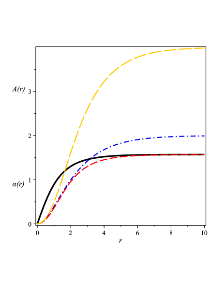
Figure 1: Numerical solutions to $\alpha\left(r\right)$ (solid black line for $m=1$ and dashed red line for $m=2$) and $A\left(r\right)$ (dot-dashed blue line for $m=1$ and long-dashed orange line for $m=2$) obtained via the first-order equations (27) and (28) in the presence of the boundary conditions (7) and (31), for $g=h=1$.

Then, in order to fulfill the finite-energy requirement $\varepsilon\left(r\rightarrow\infty\right)\rightarrow 0$, $\alpha\left(r\right)$ and $A\left(r\right)$ must behave as

$$\alpha\left(r\rightarrow\infty\right)\rightarrow\frac{\pi}{4}\text{ \ \ and \ \ }A\left(r\rightarrow\infty\right)\rightarrow 2m\text{,}$$ (42)

from which we can also calculate the energy $E_{bps}$ and the magnetic flux $\Phi_{B}$ inherent to the resulting structures, i.e.

$$E_{bps}=\mp\pi hm\text{ \ \ and \ \ }\Phi_{B}=-\frac{4\pi}{g}m\text{,}$$ (43)

($E_{bps}=\pm gh\Phi_{B}/4$) which are again quantized in terms of $m$.

Furthermore, we look for the way $\alpha\left(r\right)$ and $A\left(r\right)$ behave near the boundaries by linearizing the first-order equations (38) and (39) around the contours values in (7) and (42) (again, for simplicity, we use $m>0$), from which one gets the approximate profiles near the origin

$$\alpha\left(r\right)\approx\mathcal{C}_{1}r^{m}\text{ \ \ and \ \ }A\left(r\right)\approx\frac{\lambda}{4}r^{2}\text{,}$$ (44)

and in the limit $r\rightarrow\infty$, i.e.

$$\alpha\left(r\right)\approx\frac{\pi}{4}-\mathcal{C}_{2}e^{-\mathcal{M}_{\alpha}r}\text{ \ \ and \ \ }A\left(r\right)\approx 2m-2\mathcal{C}_{2}\sqrt{\lambda}re^{-\mathcal{M}_{A}r}\text{,}$$ (45)

with $\mathcal{M}_{\alpha}=\mathcal{M}_{A}=\sqrt{\lambda}/2$ standing for the masses of the related particles ($\mathcal{M}_{\alpha}/\mathcal{M}_{A}=1$ still holding), $\mathcal{C}_{1}$ and $\mathcal{C}_{2}$ being positive constants to be fixed via the same manner as before.

In such a scenario, given the conditions (7) and (42), the solutions $\alpha\left(r\right)$ and $A\left(r\right)$ that the equations (38) and (39) provide generate first-order vortices possessing total energy $E_{bps}=\mp\pi hm$ and magnetic flux $\Phi_{B}=-4\pi m/g$, behaving as the approximate profiles (44) and (45) in the appropriate limit.

It is interesting to note that the potential in (26) can be written as the one in (37) whether we implement the redefinitions $\alpha\rightarrow 2\alpha$, $\lambda\rightarrow\lambda/4$ and $h\rightarrow h/4$. Notwithstanding, also the first-order equations (27) and (28) reduce to those in (38) and (39) following the very same way (the corresponding energies behaving in a similar manner, the magnetic fluxes being automatically the same). We highlight that such redefinitions are completely compatible also at level of the second-order Euler-Lagrange equations.

In this sense, we argue that the $\beta\left(r\right)=\beta_{2}$ case mimics those results obtained via $\beta\left(r\right)=\beta_{1}$, both scenarios effectively describing the same phenomenology, at least concerning the first-order solitons at the classical level.

Figure 2: Numerical solutions to the magnetic field $B\left(r\right)$ for $m=1$ (solid black line), $m=3$ (dot-dashed blue line) and $m=7$ (dashed red line). The profiles are lumps centered at the origin.

We end this Section by presenting the numerical solutions we have found for $\alpha\left(r\right)$, $A\left(r\right)$, $B\left(r\right)$ and $\varepsilon_{bps}\left(r\right)$ via the first-order equations (27) and (28) in the presence of the boundary conditions (7) and (31). We have used $g=h=1$, for simplicity.

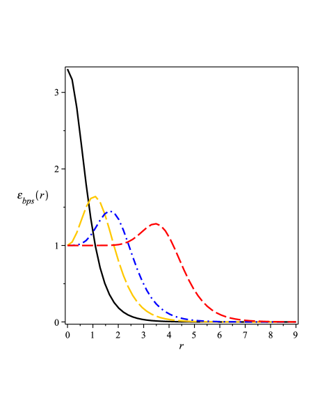
Figure 3: Numerical solutions to the energy density $\varepsilon_{bps}\left(r\right)$, conventions being the same as in the previous Figure 2 (with the long-dashed orange line for $m=2$): for $m=1$, the solution is a lump; for $m\neq 1$, the profiles are rings.

In the Figure 1, we depict the numerical solutions to the profile functions $\alpha\left(r\right)$ (solid black line for $m=1$ and dashed red line for $m=2$) and $A\left(r\right)$ (dot-dashed blue line for $m=1$ and long-dashed orange line for $m=2$). In general, these profiles reach the boundary values in a monotonic manner, behaving according the approximate solutions we have calculated previously via the linearization of the first-order equations. We also point out the way the gauge field coherently fulfills the condition $A\left(r\rightarrow\infty\right)\rightarrow 2m$, as expected.

We plot the solutions to the magnetic field $B\left(r\right)$ in the Fig. 2, for $m=1$ (solid black line), $m=3$ (dot-dashed blue line) and $m=7$ (dashed red line), all these profiles being lumps centered at the origin (the absolute value does not depending on the winding number $m$, being equal to the unity). Also, as the vorticity increases, the solutions spread over greater distances, the corresponding bosons mediating large-range interactions.

Finally, the Fig. 3 shows the profiles to the energy density $\varepsilon_{bps}\left(r\right)$, the conventions being the same ones used in the Figure 2. Here, for $m=1$, the resulting solution is a lump centered at the origin. On the other hand, for $m\neq 1$, the corresponding profiles are rings, their absolute values (amplitudes) lying on a finite distance $R$ from the origin (this way defining the ”radius” of the ring). In particular, these amplitudes (radii) decrease (increase) as the vorticity increases.

IV Conclusions and perspectives

In this work, we have considered the gauged $CP(2)$ model proposed in loginov , whilst obtaining in a coherent way the first-order vortices such model supports.

Firstly, we have detailed the planar Lagrange density defining the overall model, from which we have verified that such a system supports static solutions presenting no electric field ($A^{0}=0$ satisfying the corresponding Gauss Law identically). In the sequel, focusing our attention on those configurations presenting radial symmetry, we have implemented the well-known ansatz (4) and (5) together with convenient choices for the charges and winding numbers inherent to such maps. We have verified the constant solutions the profile function $\beta\left(r\right)$ supports, this way splitting our investigation in a priori two different branches. In addition, whilst using a very fundamental constraint, we have rewritten the radially symmetric expression for the effective energy functional in such a way highlighting the existence of a lower bound for the corresponding total energy. We have checked that the aforementioned bound is saturated when the functions $\alpha\left(r\right)$ and $A\left(r\right)$ satisfy a particular set of coupled first-order equations, also calculating the symbolic values for the total energy and the magnetic flux the final structures exhibit.

We have divided our study according the two solutions $\beta\left(r\right)$ admits. Then, whilst considering these two cases separately, we have used the fundamental constraint introduced before to obtain the particular potentials such scenarios engender, also getting the corresponding first-order equations and the appropriate boundary conditions. In view of such conditions, we have calculated explicitly the values for the energy and the magnetic flux inherent to the resulting structures. Moreover, we have concluded that the two solutions $\beta\left(r\right)$ supports in fact engender the very same phenomenology, being physically equivalent. Finally, we have plotted the numerical solutions we found for the relevant profiles, from which we have commented the general aspects they present.

It is important to emphasize that the results we have introduced in this letter hold a priori only for those radially symmetric time-independent configurations defined by the map (4) and (5). Therefore, it is not possible to assure that the gauged model (1) coherently supports a first-order framework outside that map, such question lying beyond the scope of this manuscript.

In this sense, rather natural ideas regarding new works include the search for the nontopological first-order vortices the theoretical model we have studied here possibly engenders. Furthermore, it is also interesting to consider the gauged $CP(2)$ theory when endowed by the Chern-Simons term (instead of the Maxwell one). These two possibilities are now under investigation, and we hope positive results for a future contribution.

- (1) N. Manton and P. Sutcliffe, Topological Solitons (Cambridge University Press, Cambridge, England, 2004).
- (2) E. Bogomol’nyi, Sov. J. Nucl. Phys. 24, 449 (1976). M. Prasad and C. Sommerfield, Phys. Rev. Lett. 35, 760 (1975).
- (3) H. B. Nielsen and P. Olesen, Nucl. Phys. B 61, 45 (1973).
- (4) R. Jackiw and E. J. Weinberg, Phys. Rev. Lett. 64, 2234 (1990). R. Jackiw, K. Lee and E. J. Weinberg, Phys. Rev. D 42, 3488 (1990).
- (5) D. Bazeia, E. da Hora, C. dos Santos and R. Menezes, Phys. Rev. D 81, 125014 (2010); Eur. Phys. J. C 71, 1833 (2011). D. Bazeia, R. Casana, M. M. Ferreira Jr. and E. da Hora, Europhys. Lett. 109, 21001 (2015). R. Casana, E. da Hora, D. Rubiera-Garcia and C. dos Santos, Eur. Phys. J. C 75, 380 (2015).
- (6) R. Casana, M. M. Ferreira Jr., E. da Hora and C. Miller, Phys. Lett. B 718, 620 (2012). R. Casana, M. M. Ferreira Jr., E. da Hora and A. B. F. Neves, Eur. Phys. J. C 74, 3064 (2014). R. Casana and G. Lazar, Phys. Rev. D 90, 065007 (2014). R. Casana, C. F. Farias and M. M. Ferreira Jr., Phys. Rev. D 92, 125024 (2015). R. Casana, C. F. Farias, M. M. Ferreira Jr. and G. Lazar, Phys. Rev. D 94, 065036 (2016).
- (7) L. Sourrouille, Phys. Rev. D 87, 067701 (2013). R. Casana and L. Sourrouille, Mod. Phys. Lett. A 29, 1450124 (2014).
- (8) C. Armendariz-Picon, T. Damour and V. Mukhanov, Phys. Lett. B 458, 209 (1999). V. Mukhanov and A. Vikman, J. Cosmol. Astropart. Phys. 02, 004 (2005). A. Sen, J. High Energy Phys. 07, 065 (2002). C. Armendariz-Picon and E. A. Lim, J. Cosmol. Astropart. Phys. 08, 007 (2005). J. Garriga and V. Mukhanov, Phys. Lett. B 458, 219 (1999). R. J. Scherrer, Phys. Rev. Lett. 93, 011301 (2004). A. D. Rendall, Class. Quantum Grav. 23, 1557 (2006).
- (9) M. A. Mehta, J. A. Davis and I. J. R. Aitchison, Phys. Lett. B 281, 86 (1992). B. M. A. G. Piette, D. H. Tchrakian and W. J. Zakrzewski, Phys. Lett. B 339, 95 (1994). D. H. Tchrakian and K. Arthur, Phys. Lett. B 352, 327 (1995). L. Sourrouille, A. Caso and G. S. Lozano, Mod. Phys. Lett. A 26, 637 (2011). L. Sourrouille, Mod. Phys. Lett. A 26, 2523 (2011); Mod. Phys. Lett. A 27, 1250094 (2012).
- (10) A. D’Adda, M. Luscher and P. D. Vecchia, Nucl. Phys. B 146, 63 (1978). E. Witten, Nucl. Phys. B 149, 285 (1979). A. M. Polyakov, Phys. Lett. B 59, 79 (1975). M. Shifman and A. Yung, Rev. Mod. Phys. 79, 1139 (2007).
- (11) A. Yu. Loginov, Phys. Rev. D 93, 065009 (2016).