Searching for chemical signatures of brown dwarf formation ^,

Abstract

Context. Recent studies have shown that close-in brown dwarfs in the mass range 35-55 M_Jup are almost depleted as companions to stars, suggesting that objects with masses above and below this gap might have different formation mechanisms.

Aims. We aim to test whether stars harbouring “massive” brown dwarfs and stars with “low-mass” brown dwarfs show any chemical peculiarity that could be related to different formation processes.

Methods. Our methodology is based on the analysis of high-resolution échelle spectra (R $\sim$ 57000) from 2-3 m class telescopes. We determine the fundamental stellar parameters, as well as individual abundances of C, O, Na, Mg, Al, Si, S, Ca, Sc, Ti, V, Cr, Mn, Co, Ni, and Zn for a large sample of stars known to have a substellar companion in the brown dwarf regime. The sample is divided into stars hosting massive and low-mass brown dwarfs. Following previous works a threshold of 42.5 M_Jup was considered. The metallicity and abundance trends of both subsamples are compared and set in the context of current models of planetary and brown dwarf formation.

Results. Our results confirm that stars with brown dwarf companions do not follow the well-established gas-giant planet metallicity correlation seen in main-sequence planet hosts. Stars harbouring “massive” brown dwarfs show similar metallicity and abundance distribution as stars without known planets or with low-mass planets. We find a tendency of stars harbouring “less-massive” brown dwarfs of having slightly larger metallicity, [X_Fe/Fe] values, and abundances of Sc ii, Mn i, and Ni i in comparison with the stars having the massive brown dwarfs. The data suggest, as previously reported, that massive and low-mass brown dwarfs might present differences in period and eccentricity.

Conclusions. We find evidence of a non-metallicity dependent mechanism for the formation of massive brown dwarfs. Our results agree with a scenario in which massive brown dwarfs are formed as stars. At high-metallicities, the core-accretion mechanism might become efficient in the formation of low-mass brown dwarfs while at lower metallicities low-mass brown dwarfs could form by gravitational instability in turbulent protostellar discs.

1 Introduction

Understanding whether brown dwarfs and giant planets share similar formation mechanisms is the subject of intensive studies (e.g. Luhman et al., 2007; Whitworth et al., 2007; Burgasser, 2011; Luhman, 2012; Chabrier et al., 2014).

The standard definition of a brown dwarf includes objects in a wide range of masses, from 13 to 80 Jupiter masses, with sufficient mass to ignite deuterium but below the hydrogen-burning minimum mass (Burrows et al., 1997, 2001; Chabrier & Baraffe, 2000; Spiegel et al., 2011). It is now well-established that there is a paucity of close brown dwarfs companions in comparison with gas-giant planets or binaries around main-sequence stars (Campbell et al., 1988; Murdoch et al., 1993; Marcy & Butler, 2000; Grether & Lineweaver, 2006; Sahlmann et al., 2011), usually known as the brown dwarf desert.

There have been several studies with the goal of understanding whether the properties of the brown dwarf population could be related to the formation mechanism of these objects. In a recent work, Ma & Ge (2014) compare the orbital properties (period and eccentricities) of a sample of brown dwarf companions around 65 stars. They found that while brown dwarfs with minimum masses greater than $\sim$ 42.5 M_Jup follow a similar period-eccentricity distribution to that of stellar binaries, brown dwarfs with masses below 42.5 M_Jup have an eccentricity distribution consistent with that of massive planets. This suggests that the standard definition of brown dwarf might mix two kind of objects with different formation mechanisms. The formation of high-mass brown dwarfs might be a scaled-down version of star formation through fragmentation of molecular clumps. On the other hand, less-massive brown dwarfs might form like giant-planets.

Current models of giant-planet formation can be divided into two broad categories: i) core-accretion models (e.g. Pollack et al., 1996; Rice & Armitage, 2003; Alibert et al., 2004; Mordasini et al., 2012) which are able to explain the observed gas-giant planet metallicity correlation (e.g. Gonzalez, 1997; Santos et al., 2004; Fischer & Valenti, 2005) as well as the lack of a metallicity correlation in low-mass planet hosts (e.g. Mayor et al., 2011; Cassan et al., 2012; Howard et al., 2013); and ii) disc instability models which do no depend on the metallicity of the primordial disc (Boss, 1997, 2002, 2006). If brown dwarfs form like giant-planets and those are mainly formed by core-accretion, stars hosting brown dwarfs should show the metal-enrichment seen in gas-giant planet hosts.

Several attempts to understand the metallicity distribution of stars with brown dwarfs companions have been performed. Sahlmann et al. (2011) notice that while some stars with brown dwarf companions are metal rich, others show sub-solar metallicities. Ma & Ge (2014) do not find significant metallicity differences between brown dwarf host stars with (minimum) masses below and above 42.5 M_Jup. Mata Sánchez et al. (2014) analyse in a homogeneous way the abundances of 15 stars hosting brown dwarfs (7 “candidates” and 8 “discarded” based on their Hipparcos astrometry) showing that they differ from those of stars hosting gas-giant planets. Also, they suggest higher abundances for the stars hosting brown dwarfs with masses below 42.5 M_Jup.

Given that previous works are based on small or inhomogeneous samples a detailed chemical analysis of a homogeneous and large sample of stars hosting brown dwarfs is needed before formation mechanisms of brown dwarfs are invoked. This is the goal of this paper, in which we present a homogeneous analysis of a large sample of brown dwarf hosts that is based on high resolution and high signal-to-noise ratio (S/N) échelle spectra.

This paper is organised as follows. Section 2 describes the stellar samples analysed in this work, the spectroscopic observations, and how stellar parameters and abundances are obtained. The comparison of the properties and abundances of stars with brown dwarf companions with masses larger and below 42.5 M_Jup is presented in Sect. 3, where we also include a search for correlations between the stellar and brown dwarf properties. The results are discussed at length in Sect. 4. Our conclusions follow in Sect. 5.

2 Observations

2.1 The stellar sample

A sample of stars with known brown dwarfs companions (SWBDs) with (projected) masses between 10 and 70 M_Jup was built using as reference the 65 stars listed in the recent compilation by Ma & Ge (2014) plus the 61 stars with brown dwarfs candidates listed by Wilson et al. (2016). Although different authors might have different criteria to classify an object as a brown dwarf, we note that $\sim$ 64% of the stars listed in Wilson et al. (2016) were already given in the compilation by Ma & Ge (2014). Fifteen brown dwarf companions listed in Wilson et al. (2016) were published after Ma & Ge (2014). Only seven stars listed in Wilson et al. (2016) and known before Ma & Ge (2014) were not included in this compilation, five of them have projected masses $\sim$ 10-11 M_Jup, while the other two are in the range 62-65 M_Jup. Although we do not know the reason why these seven stars were not included in Ma & Ge (2014) we we have decided to keep them in our analysis. Thus, from the above compilations, we selected all stars with spectral type between F6 and K2 (independently of its luminosity class) with high-resolution spectra available in public archives or already observed by our team in our previous programmes (see below). Several stars having a very low signal-to-noise (S/N) ratio or showing indications of high rotation were also discarded.

Our final sample consists of 53 stars with brown dwarfs, including 10 F stars, 31 G stars, and 12 K stars. Regarding their evolutionary stage, 8 stars are red giants, 19 are classified as subgiants, while 26 stars are on the main-sequence. The stars are listed in Table LABEL:parameters_table_full.

2.2 Spectroscopic data

High-resolution spectra of the stars were mainly collected from public archives: data for six stars were taken from the ELODIE (Baranne et al., 1996) archive, twenty stars from the SOPHIE (Bouchy & Sophie Team, 2006) archive, HARPS (Mayor et al., 2003) spectra from the ESO archive was used for sixteen stars, while for three stars FEROS spectra were used (Kaufer et al., 1999). For the star 11 Com a UVES (Dekker et al., 2000) spectra was taken from the ESO archive, HARPS-N spectra (Cosentino et al., 2012) were taken from the Telescopio Nazionale Galileo archive for the star KOI-415. Additional data for six stars were taken from our own observations (Maldonado et al., 2013; Maldonado & Villaver, 2016) four of them using the Nordic Optical Telescope (2.56 m) with the FIES instrument (Frandsen & Lindberg, 1999), and two stars using the MERCATOR telescope (1.2 m) with the HERMES spectrograph (Raskin et al., 2011). Table 1 summarises the properties of the different spectra.

Table 1: Properties of the different spectrographs used in this work.

Spectrograph	Spectral range (Å)	Resolving power	$N$ stars
SOPHIE	3872-6943	75000	20
HARPS	3780-6910	115000	16
ELODIE	3850-6800	42000	6
FIES	3640-7360	67000	4
FEROS	3500-9200	48000	3
HERMES	3800-9000	85000	2
HARPS-N	3830-6930	115000	1
UVES	4780-6800	110000	1

All the spectra were reduced by the corresponding pipelines which implement the typical corrections involved in échelle spectra reduction. When needed several spectra of the same star were properly combined in order to obtain a higher signal-to-noise ratio (S/N) spectra. Typical values of the S/N (measured around 605 nm) are between 70 and 200. The spectra were corrected from radial velocity shifts by using the precise radial velocities provided by the ELODIE, SOPHIE and HARPS data reduction pipelines. For the rest of the targets radial velocities were measured by cross-correlating their spectra with spectra of radial velocity standard stars of similar spectral types obtained during the same observations.

2.3 Analysis

Basic stellar parameters (T_eff, $\log g$, microturbulent velocity $\xi_{\rm t}$, and [Fe/H]) were determined by applying the iron ionisation and excitation equilibrium conditions to a set of well defined 302 Fe i and 28 Fe ii lines. The computations were done with the TGVIT (Takeda et al., 2005) code. The line list and details on the adopted parameters (excitation potential, $\log(gf)$ values) are available on Y. Takeda’s web page. ATLAS9, plane-parallel, LTE atmosphere models (Kurucz, 1993) were used in the computations. Uncertainties in the stellar parameters are obtained by changing each stellar parameter from the converged solution until the excitation equilibrium, the ionisation equilibrium or the match of the curve of growth is no longer fulfilled. We are aware that this procedure only evaluates “statistical” errors and that other systematic sources of uncertainties (i.e., the list lines used, the adopted atomic parameters, or the choice of the atmosphere model) are not taken into account (see, for details Takeda et al., 2002a, b). Zieliński et al. (2012) estimated that more realistic uncertainties might be of the order of two-three times the ones provided by TGVIT.

In order to avoid weak lines as well as errors due to uncertainties in the damping parameters only lines with measured equivalent widths (EWs) between 8 and 120 mÅ were used (e.g. Takeda et al., 2008). Stellar EWs were measured using the automatic code ARES2 (Sousa et al., 2015) adjusting the reject parameter according to the S/N ratio of the spectra as described in Sousa et al. (2008).

2.4 Photometric parameters and comparison with previous works

In order to test the reliability of our derived parameters, photometric effective temperatures were derived from the Hipparcos $(B-V)$ colours (Perryman & ESA, 1997) by using the calibration provided by Casagrande et al. (2010, Table 4). Before computation, colours were de-reddened by using the stellar galactic coordinates and the tables given by Arenou et al. (1992). Distances were obtained from the revised parallaxes provided by van Leeuwen (2007) from a new reduction of the Hipparcos’s raw data. In the few cases in which colours or parallaxes were not available we took the values provided by the Simbad database (Wenger et al., 2000). The comparison between the temperature values obtained by both procedures, spectroscopic and photometric, is shown in the left panel of Figure 1. It is clear from the figure that there is no sound systematic difference between them. Both temperatures differ in median by 21 K, with a standard deviation of 153 K.

Stellar evolutionary parameters, namely surface gravity, age, mass, and radius were computed from Hipparcos V magnitudes and parallaxes using the code PARAM (da Silva et al., 2006), which is based on the use of Bayesian methods, and the PARSEC set of isochrones by Bressan et al. (2012). The comparison between the spectroscopic and evolutionary $\log g$ values is shown in the middle panel of Figure 1. The figure reveals the known trend of spectroscopic surface gravities to be systematically larger than the evolutionary estimates (e.g. da Silva et al., 2006; Maldonado et al., 2013). Besides that, the distribution of $\log g$_spec - $\log g$_evol shows a median value of only 0.05, and a standard deviation of 0.13 consistent with previous works (da Silva et al., 2006; Maldonado et al., 2013, 2015). The outlier in upper left corner is BD+20 2457, which has a largely undetermined parallax, $\pi$ = 5.0 $\pm$ 26.0 mas (Niedzielski et al., 2009).

We finally compare our metallicities with those already reported in the literature. Values for the comparison are taken from i) the SWEETCat catalogue (Santos et al., 2013, SA13), whose parameters are mainly derived from the same authors using the iron ionisation and equilibrium conditions; ii) Valenti & Fischer (2005, VF05), where metallicities are computed by using spectral synthesis; iii) Nordström et al. (2004, NO04), which provide photometric metallicities; iv) the compilations by Ma & Ge (2014, MG14) and Wilson et al. (2016); and from v) Maldonado & Villaver (2016, MA16) as a consistency double check. The comparison is shown in the right panel of Figure 1. The agreement is overall good and no systematic differences are found with the literature estimates.

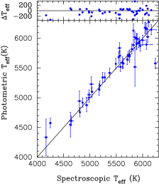
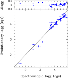
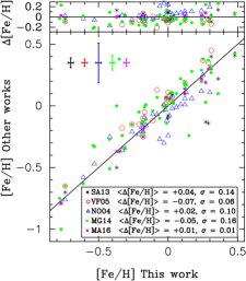
Figure 1: Spectroscopic stellar parameters derived in this work versus estimates based on photometry or values from the literature. Left: effective temperature; Middle: surface gravity $\log g$; Right: stellar metallicity [Fe/H]. The upper panels show the differences between the parameters derived in this work and the values obtained from photometry or given in the literature.

landscape

Table 2: Spectroscopic parameters with uncertainties for the stars measured in this work.

Star	MC$\sin i$⋆	Teff	$\log g$	$\xi_{t}$	[Fe/H]	Sp.†	Age	M⋆	R⋆	LC♯	Kin‡
	(MJup)	(K)	(${\rm cms^{-2}}$)	(${\rm kms^{-1}}$)	(dex)		(Gyr)	(M⊙)	(R⊙)
(1)	(2)	(3)	(4)	(5)	(6)	(7)	(8)	(9)	(10)	(11)	(12)
HD 4747	46.1 $\pm$ 2.3 a	5373 $\pm$ 20	4.66 $\pm$ 0.05	0.84 $\pm$ 0.19	-0.18 $\pm$ 0.02	5	1.53 $\pm$ 1.39	0.85 $\pm$ 0.01	0.76 $\pm$ 0.01	5	D
HD 5388	69.2 $\pm$ 19.9 a,tm	6116 $\pm$ 18	3.75 $\pm$ 0.03	1.55 $\pm$ 0.08	-0.42 $\pm$ 0.01	2	5.29 $\pm$ 0.34	1.10 $\pm$ 0.02	1.93 $\pm$ 0.07	4	D
HIP 5158	15.04 $\pm$ 10.55 a	4750 $\pm$ 35	4.71 $\pm$ 0.08	0.35 $\pm$ 0.39	0.36 $\pm$ 0.04	2	3.04 $\pm$ 3.17	0.80 $\pm$ 0.02	0.73 $\pm$ 0.02	5	D
HD 10697	38 $\pm$ 13 a,tm	5634 $\pm$ 18	4.03 $\pm$ 0.04	1.14 $\pm$ 0.16	0.12 $\pm$ 0.03	4	7.40 $\pm$ 0.22	1.11 $\pm$ 0.02	1.74 $\pm$ 0.03	4	D
HD 13189	20 a	4168 $\pm$ 25	1.63 $\pm$ 0.10	1.57 $\pm$ 0.15	-0.37 $\pm$ 0.05	4	4.50 $\pm$ 2.88	1.23 $\pm$ 0.25	33.69 $\pm$ 5.93	3	D
HD 13507	67${}^{\rm+8}_{\rm-9}$ b	5726 $\pm$ 18	4.61 $\pm$ 0.04	0.94 $\pm$ 0.10	-0.03 $\pm$ 0.02	1	1.57 $\pm$ 1.19	0.99 $\pm$ 0.02	0.91 $\pm$ 0.01	5	D
HD 14348	48.9 $\pm$ 1.6 b	6095 $\pm$ 23	4.09 $\pm$ 0.05	1.26 $\pm$ 0.09	0.17 $\pm$ 0.02	1	3.19 $\pm$ 0.10	1.31 $\pm$ 0.02	1.63 $\pm$ 0.05	4	D
HD 14651	47 $\pm$ 3.4 a	5490 $\pm$ 8	4.57 $\pm$ 0.02	0.83 $\pm$ 0.06	-0.03 $\pm$ 0.01	2	8.36 $\pm$ 2.80	0.89 $\pm$ 0.02	0.91 $\pm$ 0.03	5	TR
HD 16760	13.13 $\pm$ 0.56 a	5614 $\pm$ 15	4.61 $\pm$ 0.04	0.69 $\pm$ 0.09	-0.02 $\pm$ 0.01	1	2.78 $\pm$ 2.72	0.95 $\pm$ 0.02	0.91 $\pm$ 0.04	5	D
HD 22781	13.65 $\pm$ 0.97 a	5175 $\pm$ 15	4.57 $\pm$ 0.04	0.15 $\pm$ 0.35	-0.35 $\pm$ 0.02	1	4.14 $\pm$ 3.63	0.75 $\pm$ 0.02	0.70 $\pm$ 0.02	5	D
HD 283668	53 $\pm$ 4 b	4860 $\pm$ 25	4.65 $\pm$ 0.06	0.03 $\pm$ 0.25	-0.78 $\pm$ 0.01	1	5.90 $\pm$ 4.22	0.62 $\pm$ 0.01	0.57 $\pm$ 0.01	5	TR
HIP 21832	40.9 $\pm$ 26.2 a,tm	5570 $\pm$ 15	4.37 $\pm$ 0.04	0.87 $\pm$ 0.11	-0.61 $\pm$ 0.01	1	11.33 $\pm$ 0.30	0.74 $\pm$ 0.00	0.76 $\pm$ 0.00	5	TR
HD 30246	55.1${}^{\rm+20.3}_{\rm-8.2}$ a	5795 $\pm$ 15	4.58 $\pm$ 0.03	1.10 $\pm$ 0.07	0.12 $\pm$ 0.01	2	0.95 $\pm$ 0.81	1.07 $\pm$ 0.01	0.98 $\pm$ 0.03	5	D
HD 39091	10.27 $\pm$ 0.84 b	5941 $\pm$ 10	4.33 $\pm$ 0.02	1.15 $\pm$ 0.04	0.03 $\pm$ 0.01	2	4.96 $\pm$ 0.26	1.07 $\pm$ 0.01	1.15 $\pm$ 0.00	5	D
HD 38529	13.99 $\pm$ 0.59 a	5578 $\pm$ 43	3.78 $\pm$ 0.12	1.18 $\pm$ 0.14	0.31 $\pm$ 0.04	6	3.88 $\pm$ 0.11	1.38 $\pm$ 0.02	2.47 $\pm$ 0.07	4	D
HD 39392	13.2 $\pm$ 0.8 b	5824 $\pm$ 15	3.71 $\pm$ 0.03	1.14 $\pm$ 0.06	-0.54 $\pm$ 0.01	1	9.06 $\pm$ 1.40	0.94 $\pm$ 0.04	1.72 $\pm$ 0.14	4	TR
NGC 2423-3	10.64 $\pm$ 0.93 a	4630 $\pm$ 20	2.44 $\pm$ 0.08	1.35 $\pm$ 0.09	0.00 $\pm$ 0.04	2				3	D
HD 65430	67.8 a	5188 $\pm$ 18	4.68 $\pm$ 0.05	0.50 $\pm$ 0.28	-0.11 $\pm$ 0.02	1	10.13 $\pm$ 1.51	0.80 $\pm$ 0.01	0.79 $\pm$ 0.01	5	D
HD 72946	60.4 $\pm$ 2.2 b	6240 $\pm$ 20	4.29 $\pm$ 0.05	1.35 $\pm$ 0.12	0.03 $\pm$ 0.02	3				5	D
HAT-P-13	14.28 $\pm$ 0.28 a	5853 $\pm$ 28	4.41 $\pm$ 0.06	0.91 $\pm$ 0.15	0.48 $\pm$ 0.03	1	3.02 $\pm$ 0.35	1.22 $\pm$ 0.03	1.38 $\pm$ 0.08	4	D
HD 77065	41 $\pm$ 2 b	5039 $\pm$ 18	4.74 $\pm$ 0.05	0.07 $\pm$ 0.38	-0.42 $\pm$ 0.02	1	7.59 $\pm$ 3.69	0.71 $\pm$ 0.01	0.67 $\pm$ 0.02	5	TR
BD+26 1888	26 $\pm$ 2 b	4798 $\pm$ 40	4.54 $\pm$ 0.09	0.56 $\pm$ 0.35	0.04 $\pm$ 0.04	1	2.90 $\pm$ 3.13	0.77 $\pm$ 0.02	0.70 $\pm$ 0.02	5	D
BD+20 2457	22.7 $\pm$ 8.1 a	4249 $\pm$ 18	1.62 $\pm$ 0.08	1.58 $\pm$ 0.09	-0.77 $\pm$ 0.03	4	4.54 $\pm$ 4.06	0.40 $\pm$ 0.02	0.34 $\pm$ 0.04	3	TD
BD+20 2457	13.2 $\pm$ 4.7 a
HD 89707	53.6${}^{\rm+7.8}_{\rm-6.9}$ a	5894 $\pm$ 35	4.23 $\pm$ 0.08	1.18 $\pm$ 0.22	-0.53 $\pm$ 0.03	3	11.13 $\pm$ 0.49	0.84 $\pm$ 0.01	1.02 $\pm$ 0.02	5	TD
HD 92320	59.4 $\pm$ 4.1 a	5706 $\pm$ 10	4.64 $\pm$ 0.03	0.64 $\pm$ 0.10	-0.06 $\pm$ 0.01	1	0.78 $\pm$ 0.70	0.98 $\pm$ 0.01	0.88 $\pm$ 0.02	5	D
11 Com	19.4 $\pm$ 1.5 a	4810 $\pm$ 8	2.52 $\pm$ 0.03	1.38 $\pm$ 0.07	-0.31 $\pm$ 0.02	8	1.17 $\pm$ 0.28	2.02 $\pm$ 0.11	14.88 $\pm$ 0.36	3	TR
NGC 4349-127	20 $\pm$ 1.73 a	4439 $\pm$ 28	1.85 $\pm$ 0.11	1.58 $\pm$ 0.13	-0.18 $\pm$ 0.05	2				3	TD
HD 114762	10.99 $\pm$ 0.09 a	5851 $\pm$ 28	4.15 $\pm$ 0.05	1.25 $\pm$ 0.18	-0.74 $\pm$ 0.02	3	11.48 $\pm$ 0.01	0.85 $\pm$ 0.00	1.52 $\pm$ 0.04	5	TD
HD 122562	24 $\pm$ 2 b	4983 $\pm$ 28	3.86 $\pm$ 0.09	0.78 $\pm$ 0.16	0.31 $\pm$ 0.04	1	7.97 $\pm$ 0.97	1.12 $\pm$ 0.04	2.06 $\pm$ 0.09	4	D
HD 132032	70 $\pm$ 4 b	5954 $\pm$ 13	4.41 $\pm$ 0.03	0.98 $\pm$ 0.08	0.09 $\pm$ 0.01	1	2.87 $\pm$ 1.54	1.10 $\pm$ 0.01	1.12 $\pm$ 0.06	5	D
HD 131664	23${}^{\rm+26.0}_{\rm-5.0}$ a,tm	5882 $\pm$ 8	4.49 $\pm$ 0.02	1.09 $\pm$ 0.06	0.30 $\pm$ 0.01	2	2.12 $\pm$ 1.06	1.15 $\pm$ 0.01	1.14 $\pm$ 0.05	5	D
HD 134113	47${}^{\rm+2}_{\rm-3}$ b	5561 $\pm$ 23	3.76 $\pm$ 0.05	1.03 $\pm$ 0.10	-0.92 $\pm$ 0.02	1	10.98 $\pm$ 0.66	0.85 $\pm$ 0.02	2.01 $\pm$ 0.07	4	TD
HD 136118	12 $\pm$ 0.47 a	6163 $\pm$ 98	3.81 $\pm$ 0.19	1.32 $\pm$ 0.23	-0.17 $\pm$ 0.06	1	4.94 $\pm$ 1.05	1.12 $\pm$ 0.04	1.48 $\pm$ 0.06	4	D
HD 137759	12.7 $\pm$ 1.08 a	4647 $\pm$ 38	2.89 $\pm$ 0.14	1.16 $\pm$ 0.21	0.27 $\pm$ 0.07	6	2.07 $\pm$ 0.74	1.78 $\pm$ 0.23	11.14 $\pm$ 0.34	3	D
HD 137510	27.3 $\pm$ 1.9 a	5999 $\pm$ 43	4.13 $\pm$ 0.09	1.31 $\pm$ 0.12	0.25 $\pm$ 0.03	1	3.15 $\pm$ 0.31	1.39 $\pm$ 0.03	1.89 $\pm$ 0.06	4	D
HD 140913	43.2 a	6071 $\pm$ 115	4.80 $\pm$ 0.24	1.68 $\pm$ 0.50	-0.08 $\pm$ 0.07	1	1.62 $\pm$ 1.58	1.02 $\pm$ 0.04	0.96 $\pm$ 0.03	5	D
HD 156846	10.57 $\pm$ 0.29 b	6051 $\pm$ 13	4.00 $\pm$ 0.03	1.39 $\pm$ 0.05	0.13 $\pm$ 0.01	2	3.38 $\pm$ 0.41	1.36 $\pm$ 0.04	1.91 $\pm$ 0.05	4	D
HD 160508	48 $\pm$ 3 b	6045 $\pm$ 20	3.77 $\pm$ 0.04	1.33 $\pm$ 0.08	-0.16 $\pm$ 0.02	1	5.55 $\pm$ 0.57	1.14 $\pm$ 0.04	1.76 $\pm$ 0.13	4	D
HD 162020	14.4 $\pm$ 0.04 a	4801 $\pm$ 30	4.60 $\pm$ 0.08	0.62 $\pm$ 0.34	0.00 $\pm$ 0.04	2	3.32 $\pm$ 3.35	0.76 $\pm$ 0.02	0.70 $\pm$ 0.02	5	D
HD 167665	50.6 $\pm$ 1.7 a	6080 $\pm$ 15	4.13 $\pm$ 0.03	1.29 $\pm$ 0.08	-0.21 $\pm$ 0.01	5	6.72 $\pm$ 0.23	1.03 $\pm$ 0.01	1.32 $\pm$ 0.02	5	D
HD 168443	34.3 $\pm$ 9 a,tm	5544 $\pm$ 5	4.11 $\pm$ 0.02	1.04 $\pm$ 0.04	0.01 $\pm$ 0.01	2	10.70 $\pm$ 0.46	1.00 $\pm$ 0.01	1.54 $\pm$ 0.04	4	D
HD 174457	65.8 b	5825 $\pm$ 20	4.08 $\pm$ 0.05	1.22 $\pm$ 0.12	-0.26 $\pm$ 0.02	3	9.80 $\pm$ 0.55	0.96 $\pm$ 0.02	1.48 $\pm$ 0.07	4	D
HD 175679	37.3 $\pm$ 2.8 a	5028 $\pm$ 33	2.57 $\pm$ 0.10	1.43 $\pm$ 0.17	-0.01 $\pm$ 0.05	5	0.66 $\pm$ 0.11	2.53 $\pm$ 0.12	11.79 $\pm$ 0.80	3	D
HD 180314	22 a	4983 $\pm$ 53	3.17 $\pm$ 0.17	1.27 $\pm$ 0.21	0.24 $\pm$ 0.07	4	1.14 $\pm$ 0.24	2.13 $\pm$ 0.13	8.88 $\pm$ 0.47	3	TR
KOI-415	62.14 $\pm$ 2.69 b	5513 $\pm$ 78	4.36 $\pm$ 0.20	0.80 $\pm$ 0.31	0.15 $\pm$ 0.07	7				4
HD 190228	49.4 $\pm$ 14.8 a,tm	5241 $\pm$ 20	3.66 $\pm$ 0.05	0.96 $\pm$ 0.09	-0.33 $\pm$ 0.02	3	5.70 $\pm$ 0.69	1.12 $\pm$ 0.04	2.48 $\pm$ 0.11	4	D
HR 7672	68.7 $\pm$ 3 a,tm	5923 $\pm$ 18	4.45 $\pm$ 0.05	1.14 $\pm$ 0.12	-0.01 $\pm$ 0.02	3	3.68 $\pm$ 0.71	1.05 $\pm$ 0.02	1.05 $\pm$ 0.01	5	D
HD 191760	38.17 $\pm$ 1.02 a	5887 $\pm$ 10	4.13 $\pm$ 0.02	1.22 $\pm$ 0.05	0.24 $\pm$ 0.01	2	4.33 $\pm$ 0.57	1.23 $\pm$ 0.04	1.55 $\pm$ 0.11	4	D
HD 202206	17.5 a	5754 $\pm$ 8	4.56 $\pm$ 0.02	1.03 $\pm$ 0.05	0.29 $\pm$ 0.01	2	1.02 $\pm$ 0.83	1.10 $\pm$ 0.01	1.02 $\pm$ 0.03	5	D
HD 209262	32.3${}^{\rm+1.6}_{\rm-1.5}$ b	5753 $\pm$ 8	4.38 $\pm$ 0.02	1.02 $\pm$ 0.04	0.06 $\pm$ 0.01	2	7.48 $\pm$ 0.75	1.00 $\pm$ 0.01	1.13 $\pm$ 0.05	5	D
BD+24 4697	53 $\pm$ 3 b	4937 $\pm$ 25	4.74 $\pm$ 0.07	0.12 $\pm$ 0.46	-0.16 $\pm$ 0.03	1	5.207 $\pm$ 4.15	0.754 $\pm$ 0.016	0.705 $\pm$ 0.017	5	TR
HD 217786	13 $\pm$ 0.8 a	5882 $\pm$ 8	4.13 $\pm$ 0.02	1.18 $\pm$ 0.05	-0.19 $\pm$ 0.01	2	9.40 $\pm$ 0.22	0.96 $\pm$ 0.01	1.32 $\pm$ 0.06	4	D
HD 219077	10.39 $\pm$ 0.09 b	5284 $\pm$ 5	3.91 $\pm$ 0.02	0.94 $\pm$ 0.04	-0.18 $\pm$ 0.01	2	8.55 $\pm$ 0.25	1.03 $\pm$ 0.01	1.99 $\pm$ 0.02	4	TR

Table 2: Continued.

2.5 Abundance computation

Chemical abundance of individual elements C, O, Na, Mg, Al, Si, S, Ca, Sc, Ti, V, Cr, Mn, Co, Ni, and Zn were obtained using the 2014 version of the code MOOG (Sneden, 1973). The selected lines are taken from the list provided by Maldonado et al. (2015), with the only exception of carbon, for which we use the lines at 505.2 and 538.0 nm. For Zn abundances, the lines at 481.05 and 636.23 nm were considered.

Hyperfine structure (HFS) was taken into account for V i, and Co i abundances. HFS corrections for Mn i were not taken into account as Maldonado et al. (2015) found slightly different abundances when considering different lines. Finally, the oxygen abundance was determined from the forbidden [O i] line at 6300Å . Since this line is blended with a closer Ni i line (e.g. Allende Prieto et al., 2001), we first used the MOOG task ewfind to determine the EW of the Ni line. This EW was subtracted from the Ni i plus [O i] feature’s EW. The remaining EW was used for determining the oxygen abundance (e.g. Delgado Mena et al., 2010).

We have used three representative stars, namely HD 180314 (T_eff = 4983 K), HD 38529 (5578 K), and HD 191760 (5887 K) in order to provide an estimate on how the uncertainties in the atmospheric parameters propagate into the abundance calculation. Abundances for each of these three stars were recomputed using T_eff = T_eff + $\Delta$T_eff, T_eff - $\Delta$T_eff, and similarly for $\log g$, $\xi_{\rm t}$, and [Fe/H]. Results are given in Table 3.

Table 3: Abundance sensitivities.

	HD 180314				HD 38529				HD 191760
Ion
	$\Delta$Teff	$\Delta$$\log g$	$\Delta$[Fe/H]	$\Delta$$\xi_{t}$	$\Delta$Teff	$\Delta$$\log g$	$\Delta$[Fe/H]	$\Delta$$\xi_{t}$	$\Delta$Teff	$\Delta$$\log g$	$\Delta$[Fe/H]	$\Delta$$\xi_{t}$
	$\pm$53	$\pm$0.17	$\pm$0.07	$\pm$0.21	$\pm$43	$\pm$0.12	$\pm$0.04	$\pm$0.14	$\pm$10	$\pm$0.02	$\pm$0.01	$\pm$0.05
	(K)	(cms-2)	(dex)	(kms-1)	(K)	(cms-2)	(dex)	(kms-1)	(K)	(cms-2)	(dex)	(kms-1)
C i	0.06	0.07	$<$ 0.01	0.01	0.03	0.04	$<$ 0.01	0.01	0.01	0.01	$<$ 0.01	$<$ 0.01
O i	0.01	0.07	0.03	0.02	$<$ 0.01	0.06	0.01	0.02	$<$ 0.01	0.01	$<$ 0.01	$<$ 0.01
Na i	0.04	0.02	$<$ 0.01	0.08	0.02	0.01	$<$ 0.01	0.02	0.01	$<$ 0.01	$<$ 0.01	0.01
Mg i	0.03	0.02	0.01	0.08	0.03	0.02	$<$ 0.01	0.04	0.01	$<$ 0.01	$<$ 0.01	0.01
Al i	0.03	0.01	$<$ 0.01	0.05	0.02	0.01	$<$ 0.01	0.02	0.01	$<$ 0.01	$<$ 0.01	$<$ 0.01
Si i	0.02	0.03	0.01	0.04	$<$ 0.01	0.01	$<$ 0.01	0.02	$<$ 0.01	$<$ 0.01	$<$ 0.01	0.01
S i	0.06	0.06	$<$ 0.01	0.02	0.03	0.03	$<$ 0.01	0.01	0.01	$<$ 0.01	$<$ 0.01	$<$ 0.01
Ca i	0.05	0.03	$<$ 0.01	0.10	0.03	0.02	$<$ 0.01	0.05	0.01	$<$ 0.01	$<$ 0.01	0.01
Sc i	0.07	$<$ 0.01	$<$ 0.01	0.06	0.04	$<$ 0.01	$<$ 0.01	0.01	0.01	$<$ 0.01	$<$ 0.01	$<$ 0.01
Sc ii	$<$ 0.01	0.07	0.02	0.10	$<$ 0.01	0.05	0.01	0.05	$<$ 0.01	0.01	$<$ 0.01	0.02
Ti i	0.07	0.01	$<$ 0.01	0.11	0.05	0.01	$<$ 0.01	0.04	0.01	$<$ 0.01	$<$ 0.01	0.01
Ti ii	0.01	0.07	0.02	0.11	$<$ 0.01	0.05	0.01	0.06	$<$ 0.01	0.01	$<$ 0.01	0.02
V i	0.09	$<$ 0.01	0.01	0.03	0.05	$<$ 0.01	$<$ 0.01	$<$ 0.01	0.02	$<$ 0.01	$<$ 0.01	$<$ 0.01
Cr i	0.05	0.01	$<$ 0.01	0.09	0.03	0.01	$<$ 0.01	0.04	0.01	$<$ 0.01	$<$ 0.01	0.01
Cr ii	0.03	0.07	0.02	0.08	0.01	0.04	0.01	0.06	$<$ 0.01	0.01	$<$ 0.01	0.02
Mn i	0.04	0.02	0.01	0.14	0.03	0.01	$<$ 0.01	0.07	0.01	$<$ 0.01	$<$ 0.01	0.02
Co i	0.03	0.04	0.02	0.01	0.03	0.01	$<$ 0.01	$<$ 0.01	0.01	$<$ 0.01	$<$ 0.01	$<$ 0.01
Ni i	0.01	0.03	0.01	0.08	0.02	$<$ 0.01	$<$ 0.01	0.04	0.01	$<$ 0.01	$<$ 0.01	0.01
Zn i	0.03	0.05	0.02	0.11	0.01	0.02	0.01	0.06	$<$ 0.01	$<$ 0.01	$<$ 0.01	0.02

As final uncertainties for the derived abundances, we give the quadratic sum of the uncertainties due to the propagation of the errors in the stellar parameters, plus the line-to-line scatter errors. For abundances derived from one single line a line-to-line scatter error of 0.03 dex (the median value of all the scatter errors) was assumed. Abundances with large line-to-line scatter errors were discarded. We should caution that these uncertainties should be regarded as lower limits given that abundance estimates are affected by systematics (i.e. atmosphere models or atomic data) that are difficult to account for. Our abundances are given in Table LABEL:abundance_table_full. They are expressed relative to the solar values derived in Maldonado et al. (2015) and Maldonado & Villaver (2016) which were obtained by using similar spectra and the same methodology to the one used in this work.

A comparison of our derived abundances with those previously reported in the literature is shown in Figure 2. Whilst individual comparisons among this work and those in the literature are difficult to perform given the small number of stars in common and the different species analysed, there seems to be an overall good agreement between our estimates and previously reported values for the refractory elements. In the case of volatile elements (C, O, S, and Zn) we found few previous estimates to compare with, most likely due to the inherent difficulties in obtaining accurate abundances for these elements.

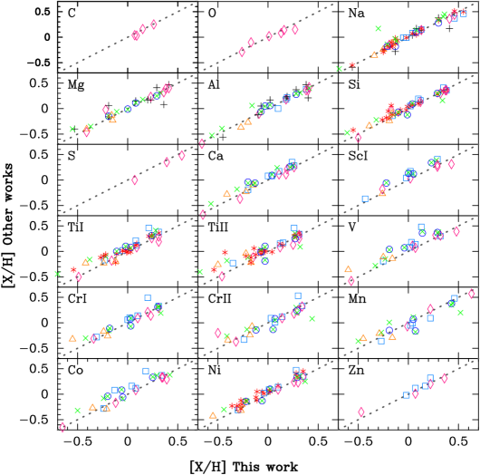
Figure 2: Comparison of our abundances to those of Beirão et al. (2005) (black $+$), Valenti & Fischer (2005) (red $\ast$), Takeda (2007) (cyan open squares), Neves et al. (2009) (blue open circles), Adibekyan et al. (2012) (green $\times$), Mata Sánchez et al. (2014) (orange open triangles) and Maldonado & Villaver (2016) (purple open diamonds).

landscape

Table 4: Derived abundances [X/H]

Star	C i	O i	Na i	Mg i	Al i	Si i	S i	Ca i	Sc i	Sc ii	Ti i	Ti ii	V i	Cr i	Cr ii	Mn i	Co i	Ni i	Zn i
HD 4747			-0.25	-0.15	-0.20	-0.19	-0.07	-0.22	-0.26	-0.27	-0.12	-0.17	-0.16	-0.20	-0.18	-0.16	-0.21	-0.27	-0.20
			0.04	0.06	0.04	0.02	0.05	0.06	0.05	0.07	0.06	0.07	0.05	0.05	0.07	0.08	0.06	0.04	0.16
HD 5388	-0.31	-0.42	-0.30	-0.37	-0.46	-0.32		-0.31		-0.51	-0.38	-0.41	-0.33	-0.42	-0.41	-0.50	-0.50	-0.44	-0.53
	0.03	0.04	0.06	0.07	0.03	0.02		0.04		0.04	0.03	0.04	0.06	0.03	0.06	0.06	0.04	0.02	0.05
HIP 5158	1.09	-0.05	0.36	0.15	0.41	0.34		0.09		0.39	0.28	0.32	0.64	0.33	0.44	0.52	0.42	0.37
	0.07	0.07	0.12	0.07	0.06	0.04		0.13		0.10	0.10	0.10	0.07	0.07	0.12	0.13	0.06	0.06
HD 10697	0.07	0.01	0.13	0.23	0.18	0.12	0.07	0.11	0.02	0.11	0.09	0.12	0.07	0.10	0.14	0.22	0.08	0.10	0.07
	0.04	0.06	0.04	0.05	0.04	0.02	0.15	0.06	0.06	0.06	0.05	0.07	0.05	0.05	0.08	0.07	0.06	0.04	0.08
HD 13189	0.15	-0.17	-0.19	-0.22	-0.09	-0.17		-0.28		-0.31	-0.16	-0.15	0.04	-0.34	-0.32	-0.01	-0.12	-0.29
	0.08	0.07	0.11	0.08	0.06	0.06		0.09		0.10	0.11	0.14	0.17	0.09	0.14	0.13	0.10	0.07
HD 13507	-0.13	-0.07	-0.17	-0.09	-0.14	-0.08	0.01	-0.04	-0.07	-0.15	-0.05	-0.08	-0.05	-0.02	-0.02	-0.13	-0.14	-0.12	-0.28
	0.07	0.04	0.03	0.03	0.05	0.02	0.04	0.04	0.03	0.05	0.03	0.05	0.06	0.03	0.05	0.06	0.05	0.03	0.04
HD 14348	0.14	0.09	0.29	0.16	0.14	0.20	0.05	0.18	0.16	0.14	0.13	0.12	0.16	0.13	0.20	0.22	0.06	0.17	0.07
	0.03	0.04	0.06	0.05	0.02	0.02	0.03	0.04	0.03	0.04	0.02	0.04	0.04	0.02	0.07	0.04	0.04	0.02	0.06
HD 14651	-0.06	0.08	-0.08	0.04	0.03	-0.03	0.02	-0.08	-0.07	-0.06	-0.02	-0.01	-0.02	-0.02	-0.02	0.04	-0.03	-0.05	-0.06
	0.07	0.05	0.05	0.06	0.03	0.02	0.05	0.06	0.05	0.06	0.05	0.07	0.05	0.05	0.08	0.07	0.06	0.04	0.08
HD 16760			-0.18	-0.14	-0.08	-0.08	-0.19	-0.06	-0.14	-0.15	-0.06	-0.05	-0.07	0.00	0.04	-0.02	-0.17	-0.09	-0.05
			0.04	0.05	0.04	0.02	0.05	0.06	0.03	0.05	0.04	0.06	0.04	0.04	0.06	0.06	0.07	0.03	0.14
HD 22781	-0.05		-0.24	-0.26	0.11	-0.28		-0.21	-0.07	-0.12	-0.05	-0.15	-0.06	-0.27	-0.25	-0.42	-0.25	-0.36	-0.18
	0.18		0.10	0.06	0.15	0.03		0.08	0.10	0.16	0.08	0.09	0.07	0.06	0.08	0.09	0.05	0.05	0.16
HD 283668	0.45		-0.75	-0.56	-0.40	-0.57		-0.53	-0.44	-0.79	-0.41	-0.51	-0.43	-0.66	-0.67	-0.95	-0.63	-0.75	-0.68
	0.07		0.10	0.07	0.06	0.04		0.08	0.07	0.09	0.09	0.10	0.08	0.08	0.09	0.11	0.05	0.06	0.09
HIP 21832	-0.48		-0.64	-0.34	-0.44	-0.46		-0.48		-0.58	-0.43	-0.43	-0.44	-0.62	-0.52	-0.79	-0.54	-0.62	-0.61
	0.05		0.05	0.09	0.04	0.02		0.06		0.06	0.05	0.07	0.09	0.05	0.07	0.08	0.04	0.04	0.07
HD 30246	0.01		0.08	0.09	0.09	0.08		0.10	0.11	0.03	0.07	0.09	0.05	0.13	0.18	0.19	-0.02	0.08	0.02
	0.05		0.03	0.03	0.03	0.02		0.04	0.04	0.04	0.03	0.04	0.04	0.03	0.04	0.06	0.09	0.02	0.11
HD 39091	-0.03	-0.01	0.08	0.08	0.02	0.04	0.05	0.04	0.00	-0.04	-0.02	-0.03	-0.04	0.03	0.07	0.05	-0.06	0.02	-0.04
	0.06	0.03	0.02	0.03	0.02	0.02	0.16	0.03	0.03	0.03	0.02	0.03	0.03	0.02	0.03	0.03	0.02	0.02	0.07
HD 38529	0.26	0.16	0.46	0.41	0.38	0.38	0.39	0.26	0.29	0.34	0.31	0.31	0.32	0.31	0.34	0.63	0.34	0.35	0.22
	0.05	0.07	0.06	0.09	0.05	0.03	0.09	0.06	0.04	0.08	0.06	0.09	0.06	0.06	0.08	0.09	0.06	0.04	0.11
HD 39392	-0.38		-0.36	-0.45	-0.48	-0.44	-0.28	-0.41		-0.64	-0.52	-0.54	-0.55	-0.56	-0.49	-0.62	-0.41	-0.56	-0.60
	0.04		0.11	0.06	0.04	0.02	0.04	0.05		0.05	0.04	0.05	0.10	0.05	0.06	0.07	0.12	0.03	0.04
NGC 2423-3	-0.10	0.03	0.10	0.26	0.10	0.09		-0.04	-0.01	-0.02	0.05	-0.17	0.07	0.01	0.02	0.32	0.04	-0.02	-0.43
	0.05	0.06	0.09	0.06	0.04	0.04		0.08	0.21	0.08	0.08	0.14	0.06	0.06	0.08	0.10	0.05	0.05	0.08
HD 65430	-0.02	-0.05	-0.11	-0.01	0.05	-0.02		-0.16	-0.05	-0.05	0.00	0.04	-0.01	-0.13	-0.05	-0.09	-0.05	-0.11	0.26
	0.06	0.06	0.05	0.07	0.04	0.03		0.07	0.08	0.08	0.07	0.09	0.06	0.07	0.09	0.09	0.05	0.05	0.08
HD 72946	0.03		0.07	-0.06	0.10	0.04	-0.05	0.01		-0.13	0.00	-0.07	0.02	0.04	0.14	0.01	-0.25	-0.01	-0.18
	0.03		0.06	0.06	0.04	0.02	0.17	0.04		0.04	0.03	0.05	0.07	0.03	0.06	0.06	0.04	0.03	0.06
HAT-P-13			0.58	0.38	0.25	0.45		0.41	0.53	0.56	0.50	0.64	0.48	0.45	0.43	0.67	0.48	0.53	0.29
			0.02	0.03	0.03	0.05		0.07	0.02	0.07	0.03	0.08	0.06	0.02	0.07	0.06	0.08	0.02	0.04
HD 77065			-0.35	-0.28	-0.16	-0.27		-0.41	-0.23	-0.33	-0.15	-0.22	-0.21	-0.40	-0.30	-0.53	-0.30	-0.41	-0.21
			0.06	0.08	0.04	0.03		0.08	0.10	0.09	0.08	0.09	0.07	0.07	0.09	0.10	0.06	0.05	0.08
BD+26 1888	0.86	0.05	0.07	-0.16	0.25	0.01		-0.06	0.26	-0.02	0.12	0.09	0.20	0.03	0.05	0.13	0.10	0.04	0.09
	0.07	0.07	0.08	0.07	0.15	0.04		0.08	0.18	0.10	0.09	0.14	0.07	0.07	0.11	0.11	0.05	0.06	0.15
BD+20 2457		-0.26	-0.81	-0.41	-0.66	-0.50		-0.65	-0.74	-0.70	-0.49	-0.46	-0.57	-0.75	-0.50	-1.00	-0.65	-0.82	-0.73
		0.07	0.11	0.11	0.05	0.06		0.10	0.16	0.10	0.10	0.13	0.08	0.08	0.21	0.14	0.06	0.06	0.10
HD 89707	-0.62		-0.34	-0.41		-0.39		-0.41		-0.61	-0.42	-0.50	-0.60	-0.55	-0.40	-0.45		-0.55	-0.49
	0.03		0.07	0.12		0.03		0.05		0.03	0.06	0.05	0.04	0.05	0.04	0.09		0.03	0.04
HD 92320	-0.17		-0.16	-0.07		-0.13		-0.09	-0.13	-0.12	-0.09	-0.06	-0.15	-0.07	-0.02	-0.06	-0.23	-0.14	-0.16
	0.04		0.04	0.05		0.02		0.06	0.04	0.05	0.04	0.05	0.05	0.03	0.06	0.09	0.03	0.03	0.06
11 Com	-0.45	-0.12	-0.05	-0.19	-0.12	-0.16	-0.01	-0.20	-0.43	-0.25	-0.23	-0.35	-0.25	-0.31	-0.24	-0.27	-0.24	-0.30	-0.37
	0.08	0.08	0.08	0.09	0.06	0.05	0.09	0.11	0.21	0.12	0.12	0.19	0.10	0.10	0.11	0.15	0.08	0.07	0.15
NGC 4349-127	-0.20	-0.21	0.23	0.05	-0.12	0.07	0.69	-0.14		-0.23	-0.19	-0.07	-0.06	-0.17	-0.19	0.03	-0.13	-0.20
	0.08	0.07	0.18	0.08	0.05	0.06	0.08	0.10		0.12	0.10	0.16	0.10	0.09	0.11	0.15	0.07	0.07
HD 114762	-0.51		-0.56	-0.53	-0.45	-0.55		-0.52		-0.72	-0.54	-0.54	-0.64	-0.72	-0.57	-0.92		-0.75	-0.66
	0.01		0.05	0.10	0.03	0.03		0.05		0.05	0.04	0.05	0.09	0.03	0.06	0.14		0.03	0.02
HD 122562	0.40	-0.05	0.54	0.43	0.49	0.49		0.22		0.37	0.32	0.33	0.43	0.31	0.34	0.73	0.52	0.39	0.49
	0.09	0.08	0.10	0.09	0.08	0.05		0.10		0.13	0.12	0.18	0.09	0.10	0.14	0.17	0.14	0.07	0.20
	0.07		0.13	0.07	0.05	0.04		0.09	0.13	0.09	0.09	0.10	0.07	0.07	0.09	0.12	0.10	0.06	0.09
HD 132032	0.10	0.44	0.21	0.11	0.09	0.09	0.21	0.05	0.02	0.02	0.03	0.06	0.02	0.09	0.05	0.16	0.03	0.09	0.08
	0.02	0.03	0.08	0.02	0.03	0.02	0.03	0.04	0.03	0.04	0.02	0.03	0.04	0.02	0.07	0.03	0.07	0.02	0.11
HD 131664	0.24	0.10	0.35	0.33	0.32	0.32	0.27	0.25	0.28	0.28	0.26	0.27	0.30	0.31	0.28	0.44	0.29	0.32
	0.02	0.03	0.02	0.02	0.02	0.02	0.03	0.04	0.02	0.03	0.02	0.03	0.03	0.02	0.05	0.03	0.05	0.02
HD 134113	-0.53		-0.69	-0.55	-0.56	-0.61		-0.57		-0.92	-0.70	-0.68	-0.82	-0.93	-0.83	-1.17	-0.83	-0.90	-0.79
	0.06		0.08	0.09	0.04	0.02		0.08		0.08	0.06	0.08	0.10	0.07	0.09	0.11	0.05	0.04	0.07
HD 136118	-0.58					-0.20	-0.78	-0.13		-0.39	-0.01	-0.43	-0.27	-0.10		-0.11	-0.08	-0.27	-0.81
	0.04					0.09	0.04	0.06		0.06	0.09	0.10	0.11	0.09		0.07	0.10	0.05	0.05
HD 137759		0.27	0.41	0.36	0.40	0.37		0.18		0.36	0.31	0.25	0.48	0.23	0.26	0.81	0.39	0.30
		0.08	0.09	0.09	0.05	0.06		0.11		0.12	0.12	0.16	0.10	0.10	0.12	0.17	0.08	0.07
HD 137510	0.28		0.55	0.21		0.35	0.20	0.24		0.32	0.21	0.26	0.13	0.20	0.30	0.46	0.18	0.28
	0.03		0.03	0.09		0.02	0.03	0.06		0.05	0.03	0.05	0.07	0.02	0.03	0.05	0.07	0.02
HD 140913		0.56	-0.13	-0.35	-0.16	-0.17	-0.07	-0.55		-0.23	0.02	-0.14	0.05	-0.04	0.04	0.21	0.05	-0.11	-0.47
		0.04	0.06	0.04	0.04	0.10	0.04	0.18		0.05	0.08	0.11	0.08	0.14	0.10	0.06	0.15	0.06	0.05
HD 156846	0.09		0.24	0.15		0.16		0.14		0.12	0.10	0.12	0.07	0.11	0.17	0.16	0.08	0.13	0.04
	0.03		0.06	0.03		0.02		0.04		0.03	0.02	0.03	0.04	0.02	0.04	0.04	0.03	0.02	0.05
HD 160508	-0.09		-0.08	-0.15	-0.30	-0.12		-0.06		-0.27	-0.21	-0.21	-0.14	-0.17	-0.13	-0.23	-0.23	-0.19	-0.28
	0.02		0.06	0.05	0.03	0.06		0.04		0.05	0.03	0.04	0.06	0.03	0.06	0.05	0.10	0.02	0.04
HD 162020	0.69		-0.13	-0.19	-0.07	-0.01		-0.20	0.05	-0.13	0.03	-0.03	0.14	0.03	0.05	0.07	-0.05	-0.06	-0.04
	0.06		0.06	0.06	0.05	0.03		0.12	0.14	0.08	0.07	0.09	0.07	0.06	0.09	0.09	0.04	0.05	0.09
HD 167665	-0.09		-0.16	-0.16	-0.27	-0.16	-0.21	-0.15		-0.28	-0.24	-0.22	-0.25	-0.24	-0.16	-0.29	-0.35	-0.26	-0.32
	0.02		0.07	0.08	0.06	0.02	0.18	0.04		0.03	0.02	0.03	0.06	0.03	0.05	0.05	0.06	0.02	0.09
HD 168443	0.14	0.12	0.04	0.20	0.19	0.10	0.01	0.04	0.02	0.08	0.08	0.15	0.03	0.02	0.03	0.04	0.04	0.01	0.17
	0.05	0.06	0.04	0.05	0.03	0.02	0.05	0.06	0.05	0.07	0.06	0.08	0.05	0.05	0.08	0.08	0.05	0.04	0.20
HD 174457	-0.06		-0.18	-0.21	-0.09	-0.22	-0.27	-0.18		-0.29	-0.22	-0.12	-0.16	-0.17	-0.18	-0.28	-0.23	-0.31	-0.42
	0.02		0.06	0.06	0.08	0.01	0.11	0.04		0.06	0.02	0.13	0.05	0.06	0.08	0.07	0.02	0.02	0.06
HD 175679	-0.26	-0.09	0.19	0.09	0.01	0.07	0.20	0.02	-0.24	-0.10	-0.08	0.01	-0.10	-0.06	0.07	0.20	-0.09	-0.08
	0.06	0.07	0.08	0.07	0.07	0.04	0.08	0.08	0.13	0.10	0.09	0.13	0.08	0.07	0.17	0.11	0.06	0.06
HD 180314	0.09	0.13		0.38	0.41	0.32	0.54	0.19	0.29	0.31	0.24	0.31	0.27	0.20	0.30	0.79	0.35	0.26	0.36
	0.09	0.09		0.09	0.13	0.06	0.13	0.12	0.20	0.13	0.13	0.17	0.10	0.10	0.13	0.16	0.08	0.08	0.19
KOI-415	0.24		0.17		0.61	0.06		0.16	0.30	0.24	0.36		0.60	0.19		-0.31	0.48	0.08	0.34
	0.19		0.15		0.10	0.06		0.09	0.05	0.07	0.07		0.08	0.07		0.10	0.13	0.05	0.06
HD 190228	-0.38		-0.24	-0.19	-0.10	-0.26	-0.12	-0.28	-0.38	-0.31	-0.27	-0.17	-0.31	-0.36	-0.38	-0.25	-0.29	-0.36	-0.12
	0.07		0.10	0.06	0.11	0.04	0.07	0.08	0.06	0.12	0.09	0.17	0.08	0.07	0.09	0.12	0.05	0.06	0.10
HR 7672	0.11		-0.02	-0.02	0.10	0.02	0.00	0.00	-0.02	-0.10	-0.05	-0.07	0.01	0.00	0.07	0.02	-0.13	-0.04	-0.02
	0.04		0.04	0.05	0.16	0.02	0.14	0.05	0.04	0.05	0.04	0.05	0.05	0.04	0.09	0.06	0.05	0.03	0.11
HD 191760	0.24	0.44	0.35	0.30	0.28	0.28	0.18	0.23	0.22	0.27	0.20	0.23	0.22	0.25	0.21	0.36	0.23	0.27	0.22
	0.01	0.03	0.01	0.01	0.02	0.01	0.05	0.04	0.01	0.02	0.01	0.03	0.02	0.01	0.04	0.03	0.04	0.01	0.08
HD 202206	0.16	0.14	0.30	0.29	0.28	0.29	0.18	0.22	0.23	0.25	0.24	0.27	0.29	0.30	0.29	0.43	0.25	0.29	0.17
	0.04	0.04	0.02	0.03	0.02	0.02	0.07	0.04	0.03	0.04	0.03	0.04	0.04	0.03	0.04	0.05	0.04	0.02	0.12
HD 209262	0.04	-0.17	0.08	0.17	0.12	0.07	0.14	0.04	0.00	0.04	0.03	0.06	0.04	0.07	0.08	0.13	0.04	0.05	0.02
	0.05	0.04	0.02	0.06	0.02	0.02	0.04	0.04	0.04	0.04	0.03	0.04	0.03	0.03	0.04	0.04	0.04	0.02	0.10
BD+24 4697	0.42		-0.38	-0.26	-0.16	-0.18		-0.23	-0.14	-0.30	-0.10	-0.15	-0.07	-0.17	-0.10	-0.19	-0.06	-0.20	-0.27
HD 217786	-0.08	-0.25	-0.12	-0.11	-0.16	-0.15		-0.15		-0.25	-0.22	-0.20	-0.23	-0.19	-0.21	-0.27	-0.24	-0.21	-0.23
	0.01	0.03	0.02	0.05	0.03	0.01		0.04		0.03	0.01	0.02	0.03	0.01	0.08	0.03	0.04	0.01	0.05
HD 219077	-0.13	-0.06	-0.21	0.00	-0.03	-0.10	0.03	-0.13	-0.22	-0.14	-0.11	-0.07	-0.19	-0.18	-0.12	-0.19	-0.20	-0.22
	0.06	0.07	0.06	0.06	0.05	0.03	0.07	0.08	0.07	0.09	0.08	0.09	0.07	0.07	0.09	0.10	0.06	0.05

Table 4: continued.

3 Results

3.1 Abundance patterns of stars with brown dwarfs

Recent studies (Sahlmann et al., 2011; Ma & Ge, 2014; Mata Sánchez et al., 2014) have suggested that the formation mechanisms of BDs companions with masses above and below $\sim$ 42.5 M_Jup may be different. Therefore, we have divided the sample of stars with brown dwarfs in stars with BDs candidates in the mass range M_C$\sin i$ $<$ 42.5 M_Jup and stars with BDs candidates with masses M_C$\sin i$ $>$ 42.5 M_Jup .

The SWBDs with candidates in the mass range M_C$\sin i$ $<$ 42.5 M_Jup is composed of 32 stars, including 4 F stars, 19 G stars and 9 K stars. Regarding its evolutionary state 8 are giants, 12 are classified as subgiants, and 12 stars are on the main-sequence. The total number of stars in the SWBDs with M_C$\sin i$ $>$ 42.5 M_Jup is 21, including 6 F stars, 12 G stars and 3 K stars. The sample is composed of 14 main-sequence stars as well as 7 stars in the subgiant branch. In the following we compare the metallicities and abundances of these two subsamples.

3.1.1 Stellar biases

Before a comparison of the metallicities and individual abundances between the two defined samples of stars with brown dwarfs candidates is done, a comparison of the stellar properties of both samples was performed, in particular in terms of age, distance, and kinematics, since these parameters are most likely to reflect the original metal content of the molecular cloud where the stars were born. The comparison is shown in Table 5. A series of two-sided Kolmogorov-Smirnov (K-S) tests (e.g. Peacock, 1983) were performed to check whether the samples are likely or not drawn from the same parent population. The comparison shows that both samples show similar distributions in brightness and age. The sample of SWBDs with M_C$\sin i$ $<$ 42.5 M_Jup contains stars out to larger distances and slightly larger stellar masses than the SWBDs with M_C$\sin i$ $>$ 42.5 M_Jup. Nevertheless, we note that the median distance for both samples are quite similar and most of the stars, $\sim$ 75% with M_C$\sin i$ $<$ 42.5 M_Jup are within 92 pc (the volume covered by the SWBDs with companions above 42.5 M_Jup). As a further check, the metallicity-distance plane was explored finding no metallicity difference between the SWBDs with M_C$\sin i$ $<$ 42.5 M_Jup located closer and farther than 92 pc. This potential bias is discussed with more detail in Sec. 3.1.6. Regarding the stellar mass, only four SWBDs with M_C$\sin i$ $<$ 42.5 M_Jup show stellar masses larger than 1.4 M_⊙ (SWBDs with companions above 42.5 M_Jup cover up to 1.31 M_⊙) showing a large range of metallicities (two stars have [Fe/H] $\sim$ +0.25, one shows solar metallicity, and the other one is metal-poor with [Fe/H] $\sim$ -0.30). We note that in the sample of SWBDs with M_C$\sin i$ $>$ 42.5 M_Jup there are no giant stars, indeed nearly all stars ($\sim$ 67%) are in the main-sequence. However, in its less massive counterpart sample, most of the stars are evolved, with about 62.5% of the stars in the giant and subgiant phase. This fact should be analysed carefully, since it has been shown that unlike their main-sequence counterparts, it is still unclear whether giant stars with planets show or not metal-enrichment (Sadakane et al., 2005; Schuler et al., 2005; Hekker & Meléndez, 2007; Pasquini et al., 2007; Takeda et al., 2008; Ghezzi et al., 2010; Maldonado et al., 2013; Mortier et al., 2013; Jofré et al., 2015; Reffert et al., 2015; Maldonado & Villaver, 2016). Further, the abundance of some elements might be influenced by 3D or nLTE effects (e.g. Bergemann et al., 2011; Mashonkina et al., 2011). The metallicity distribution of SWBDs with M_C$\sin i$ $<$ 42.5 M_Jup is shown in Figure 3 where the stars are classified according to their luminosity class. The figure does not reveal any clear difference in metallicity between giants, subgiants, and main-sequence stars. We will discuss this issue in more detail in Sec. 3.1.5.

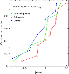
Figure 3: Histogram of cumulative frequencies for SWBDs with companions in the mass range M_C$\sin i$ $<$ 42.5 M_Jup according to their luminosity class.

3.1.2 Kinematic biases

Regarding kinematics, stars were classified as belonging to the thin/thick disc applying the methodology described in Bensby et al. (2003, 2005). For this purpose, we first computed the stellar spatial Galactic velocity components $(U,V,W)$ using the methodology described in Montes et al. (2001) and Maldonado et al. (2010), using the Hipparcos parallaxes (van Leeuwen, 2007) and Tycho-2 proper motions (Høg et al., 2000). Radial velocities were taken from the compilation of Kharchenko et al. (2007). The results show that most of the stars in both subsamples ($\sim$ 72%, and $\sim$ 75%, respectively) should, according to their kinematics, belong to the thin disc.

Another potential bias comes from the fact that several stars might harbour additional companions in the planetary range. Five SWBDs in the mass domain M_C$\sin i$ $<$ 42.5 M_Jup are known to host, in addition to a brown dwarf, at least one companion in the gas-giant planetary mass domain. These stars are HD 38529, HD 168443, HIP 5158, and HAT-P-13 (all with the planet closer to the star than the brown dwarf), and HD 2022206, where the brown dwarf occupies the innermost orbit. We note that all these stars, except one (HD 168443), show significant positive metallicities. In order to test whether this fact could affect our results we compared the metallicity distribution of SWBDs with M_C$\sin i$ $<$ 42.5 M_Jup when all the 32 stars with companions in this mass range are considered and when the four stars with possible additional planets are excluded. The results from the K-S test show that both distributions are virtually equal with a probability of $\sim$ 99%. Further analysis of this potential bias will be provided in Sec. 3.1.5. Finally, we note that only one star (BD+20 2457) harbours two companions in the brown dwarf regime.

Table 5: Comparison between the properties of SWBDs with M_C$\sin i$ $<$ 42.5 M_Jup and SWBDs with M_C$\sin i$ $>$ 42.5 M_Jup.

	MC$\sin i$ $<$ 42.5 MJup			MC$\sin i$ $>$ 42.5 MJup			K-S test
	Range	Mean	Median	Range	Mean	Median	$D$	$p$
V (mag)	3.29/10.82	7.70	7.78	5.80/9.77	7.70	7.68	0.24	0.40
Distance (pc)	18.3/2174	166.9	46.58	17.8/92.3	44.4	44.9	0.26	0.31
Age (Gyr)	0.66/11.48	5.07	4.33	0.78/11.13	5.31	5.29	0.25	0.43
Mass (M${}_{\odot})$	0.40/2.53	1.15	1.10	0.62/1.31	0.97	0.99	0.31	0.16
Teff (K)	4168/6163	5330	5570	4860/6240	5697	5795	0.34	0.08
SpType(%)	13 (F); 59 (G); 28 (K)			29 (F); 57 (G); 14 (K)
LC(%)†	25 (G); 37.5 (S); 37.5 (MS)			33 (S); 67 (MS)
D/TD(%)‡	72 (D); 9 (TD); 19 (R)			75 (D); 10 (TD); 15 (R)
† MS: Main-sequence, S: Subgiant, G: Giant
‡ D: Thin disc, TD: Thick disc, R: Transition

3.1.3 Metallicity distributions

As mentioned before 32 SWBDs are in the mass range M_C$\sin i$ $<$ 42.5 M_Jup whilst 21 stars host BDs candidates with masses M_C$\sin i$ $>$ 42.5 M_Jup. Some statistical diagnostics for both samples are summarised in Table 6, while their metallicity cumulative distribution functions are shown in Figure 4. We also show the metallicity distribution of the whole sample of stars with brown dwarfs (i.e., all the 53 stars with brown dwarf companions, SWBDs). In addition, several samples are overplotted for comparison: i) a sample of stars without known planetary companions (180 stars, SWOPs), ii) a sample of stars with known gas-giant planets (44 stars, SWGPs), and iii) a sample of stars with known low-mass planets ( M${}_{\rm p}\sin i$ $<$ 30 M_⊕, 17 stars, SWLMPs). In order to be as homogeneous as possible, these comparison samples were taken from Maldonado et al. (2015) so their stellar parameters are determined with the same technique used in this work and using similar spectra.

Table 6: [Fe/H] statistics of the stellar samples.

Sample	$Mean$	$Median$	$\sigma$	$Min$	$Max$	$N$
SWBDs	-0.10	-0.03	0.32	-0.92	0.48	53
BDs MC$\sin i$ $<$ 42.5 MJup	-0.04	0.01	0.33	-0.77	0.48	32
BDs MC$\sin i$ $>$ 42.5 MJup	-0.18	-0.11	0.28	-0.92	0.17	21
SWOPs	-0.10	-0.07	0.24	-0.87	0.37	180
SWGPs	0.12	0.10	0.18	-0.25	0.50	44
SWLMPs	-0.03	-0.01	0.23	-0.38	0.42	17

There are a few interesting facts to be taken from the distributions shown in Figure 4: i) SWBDs as a whole (magenta line) do not follow the well trend of SWGPs (light-blue line) of showing metal-enrichment; ii) considering the global metallicity distribution of SWBDs, there is a trend of SWBDs in the mass domain M_C$\sin i$ $<$ 42.5 M_Jup (dark-blue line) of having larger metallicities than SWBDs with M_C$\sin i$ $>$ 42.5 M_Jup (red line); iii) for metallicities below approximately -0.20 the metallicity distributions of SWBDs with masses above and below 42.5 M_Jup seem to follow a similar trend; iv) for larger metallicities the distribution of SWBDs with companions in the mass range M_C$\sin i$ $<$ 42.5 M_Jup clearly shifts towards higher metallicities when compared with the distribution of SWBDs in the mass range M_C$\sin i$ $>$ 42.5 M_Jup. We also note that at high-metallicities, (larger than +0.20), the metallicity distribution of of SWBDs in the mass domain M_C$\sin i$ $<$ 42.5 M_Jup is similar to that of SWGPs.

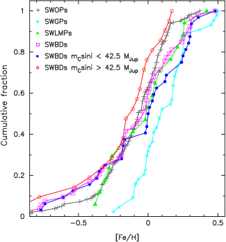
Figure 4: Histogram of cumulative frequencies for the different samples studied in this work.

These results can be compared with previous studies. Ma & Ge (2014) and Mata Sánchez et al. (2014) found that the stars with brown dwarfs companions do not show the metal-rich signature seen in stars hosting gas-giant planets. Further, Ma & Ge (2014) did not report metallicity differences between stars with BDs with minimum masses lower and larger than 42.5 M_Jup. We also note that Figure 6 in Ma & Ge (2014) shows results similar to ours: Around metallicities $\sim$ +0.00 stars with BDs with M_C$\sin i$ $<$ 42.5 M_Jup tend to show larger metallicities “reaching” the metallicity distribution of stars with gas-giant planets at [Fe/H] $\sim$ +0.25.

3.1.4 Other chemical signatures

In order to try to disclose differences in the abundances of other elements besides iron, Figure 5 compares the cumulative distribution of [X/Fe] between SWBDs with M_C$\sin i$ below and above 42.5 M_Jup. Table 7 gives some statistic diagnostics, the results of a K-S test for each ion and also for [X_α/Fe], [X_Fe/Fe], and [X_vol/Fe] (see definitions below). For Ca i, Sc i, Ti i, Cr i, and Cr ii the distributions of both samples seem to be quite similar. Indeed the the probabilities of both samples coming from the same distribution returned by the K-S tests for these ions are high ($>$ 80%). On the other hand, for the abundances of Sc ii, Mn i, Ni i, and X_Fe the tests conclude that both samples might be different.

Table 7: Comparison between the elemental abundances of stars with BDs with minimum masses M_C$\sin i$ $<$ 42.5 M_Jup and M_C$\sin i$ $>$ 42.5 M_Jup.

[X/Fe]	MC$\sin i$ $<$ 42.5 MJup		MC$\sin i$ $>$ 42.5 MJup		K-S test
	Median	$\sigma$	Median	$\sigma$	$D$	$p$-value	neff
C i	0.00	0.29	0.07	0.32	0.19	0.80	11.15
O i	-0.04	0.21	0.06	0.26	0.38	0.34	5.25
Na i	0.10	0.12	0.03	0.11	0.26	0.32	12.35
Mg i	0.10	0.14	0.03	0.13	0.40	0.03	12.16
Al i	0.07	0.13	0.00	0.17	0.35	0.09	11.48
Si i	0.08	0.08	0.03	0.10	0.29	0.19	12.68
S i	0.02	0.30	0.01	0.09	0.29	0.53	6.68
Ca i	0.01	0.10	0.01	0.15	0.13	0.97	12.68
Sc i	-0.02	0.12	-0.01	0.12	0.20	0.87	7.88
Sc ii	0.03	0.09	-0.07	0.07	0.45	0.01	12.68
Ti i	0.02	0.11	0.04	0.11	0.12	0.99	12.68
Ti ii	0.00	0.12	0.01	0.10	0.21	0.62	12.31
V i	0.02	0.13	0.02	0.13	0.20	0.63	12.68
Cr i	0.00	0.03	0.00	0.04	0.17	0.85	12.68
Cr ii	0.04	0.06	0.06	0.05	0.15	0.94	12.16
Mn i	0.09	0.19	0.00	0.15	0.45	0.01	12.68
Co i	0.03	0.09	-0.03	0.14	0.37	0.05	12.16
Ni i	0.00	0.04	-0.03	0.03	0.48	$<$0.01	12.68
Zn i	-0.04	0.19	-0.10	0.17	0.36	0.09	11.20
$X_{\alpha}$	0.04	0.09	0.01	0.10	0.23	0.45	12.68
$X_{\rm Fe}$	0.03	0.06	-0.03	0.04	0.47	$<$0.01	12.68
$X_{\rm vol}$	0.05	0.15	0.03	0.12	0.19	0.73	12.68

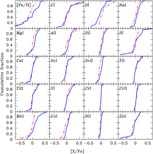
Figure 5: [X/Fe] cumulative fraction of SWBDs with M_C$\sin i$ $<$ 42.5 M_Jup (blue continuous line) and M_C$\sin i$ $>$ 42.5 M_Jup (red dash-to-dot line).

In order to compare with the SWOP, SWGP, and SWLMP samples defined in Sec. 3.1.3, we grouped the ions into three categories: alpha elements, iron-peak elements, and volatile elements. For alpha and iron-peak elements we follow Mata Sánchez et al. (2014) and define [X_α/Fe] as the mean of the [X/Fe] abundances of Mg i, Si i, Ca i, and Ti i, while [X_Fe/Fe] is defined as the mean of the Cr i, Mn i, Co i, and Ni i abundances. We define the mean volatile abundance, [X_vol/Fe] as the mean of the [X/Fe] values of the elements with a condensation temperature, T_C, lower than 900 K namely, C i, O i, S i, and Zn i. Although Na i has a T_C slightly above 900 K we include it in the group of volatiles to account for the fact that for some stars the abundances of some volatiles were not obtained. It is important to mention at this point that the abundances in the comparison samples for this work were derived in a similar way by Maldonado et al. (2015); Maldonado & Villaver (2016).

The different cumulative functions are shown in Figure 6. Interestingly, the figure reveals a tendency of SWBDs in the low-mass domain to have slightly larger abundances than the rest of the samples in all categories. In order to test this tendency the SWBDs with companions in the mass range M_C$\sin i$ $<$ 42.5 M_Jup was compared (by means of a K-S test) with the rest of the samples. The results are provided in Table 8.

Regarding $\alpha$ elements, the sample of stars with low-mass BDs companions does not seem to be different from the SWOP and SWLMP samples, although we note the low $p$-value of 0.05 when comparing with the SWOP sample. The K-S test suggests, however, that the sample differs from the one of stars harbouring gas-giant planets ($p$-value $<$ 0.01). Since this is somehow a surprising result, we have checked if our SWGP sample occupies the same place in the [X_α/Fe] vs. [Fe/H] plot as other samples in the literature. For this check we have taken the data from Adibekyan et al. (2012) finding consistent results, i.e, both our SWGP and the stars with giant planets from Adibekyan et al. (2012) tend to show high metallicity values and rather low [X_α/Fe] values. The most significant differences appear when considering the iron-peak elements. In this case the sample of SWBDs in the low-mass companion range seems to be shifted towards higher metallicities when compared with the SWOPs. No statistically significant differences are found when considering the volatile elements, although we note that in the comparison with the SWGPs the $p$-value is relatively low (of only 0.04).

We therefore conclude that the SWBD sample with companions in the mass range M_C$\sin i$ $<$ 42.5 M_Jup may differ from the SWOPs in iron-peak elements, but also from the GWPs when considering $\alpha$ elements.

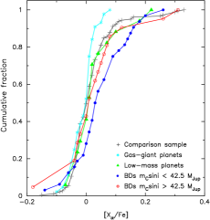
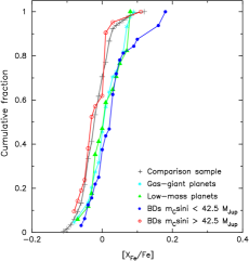
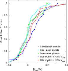
Figure 6: Histogram of cumulative frequencies of [X_α/Fe] (left), [X_Fe/Fe] (middle), and [X_vol/Fe] (right) for the different samples studied in this work.

Table 8: Comparison between the abundances of stars with BDs with minimum masses M_C$\sin i$ $<$ 42.5 M_Jup and the stars without planets, stars with low-mass planets, and stars with gas-giant planets samples.

	Stars without		Stars with low-		Stars with gas-
	planets		mass planets		giant planets
$[X/Fe]$	$D$	$p$-value	$D$	$p$-value	$D$	$p$-value
$X_{\alpha}$	0.25	0.05	0.30	0.23	0.43	$<$ 0.01
$X_{\rm Fe}$	0.40	$<$ 0.01	0.19	0.78	0.17	0.63
$X_{\rm vol}$	0.21	0.16	0.30	0.21	0.31	0.04

3.1.5 Presence of red giants and additional planetary companions

As already pointed out, 25% of the stars in the sample with low-mass brown dwarfs companions are red giants. To check for possible biases we have repeated the comparison of the abundance properties ([Fe/H], [X_α/Fe], [X_Fe/Fe], [X_vol/Fe]) of the SWBD with companions with masses above and below 42.5 M_Jup, excluding from the analysis all stars classified as giants. The results are shown in Table 9 where the new analysis is compared with the previous one. It can be seen that the results do not change in a significant way. For example, for [Fe/H] the $p$-value changes from 0.08 to 0.05, while when considering [X_Fe/Fe] it moves from less than 0.01 to 0.04. Although the threshold of 0.02 on the $p$-value is usually assumed to consider statistical significance when interpreting the results from the K-S tests, we note that a $p$-value of 0.04 is still very low. We conclude that the presence of giant stars in the SWBDs with companions below 42.5 M_Jup does not introduce any significant bias in the comparisons performed in this work.

However, the results might change if in addition to the giant stars we also exclude the subgiant stars (from both SWBDs subsamples). In this case, the $p$-value for [Fe/H] increases from 0.08 up to 0.24, while for [X_Fe/Fe] it rises from less than 0.01 up to a value of 0.64. This is in contrast to what we found when excluding only the giant stars from the analysis and may, at least partially, be due to the significant reduction of the sample size. Note that by excluding both giant and subgiant stars from the analysis we are reducing the sample to approximately half the original size.

Finally, we analyse the results when the stars with additional companions in the planetary mass are excluded (all of them in the sample of stars with low-mass brown dwarfs), see Table 9. In this case the significance of a possible metallicity difference between SWBDs with companions above and below 42.5 M_Jup diminishes (the $p$-value changes from 0.08 to 0.31). The $p$-value for [X_Fe/Fe] also rises a bit from less than 0.01 to 0.03. We again conclude that no significant bias is introduced by the five SWBDs with companions below 42.5 M_Jup that, in addition to a brown dwarf companion, also harbours a companion in the gas-giant planetary mass domain.

Table 9: Comparison between the abundances of stars with BDs with minimum masses M_C$\sin i$ $>$ 42.5 M_Jup and stars with BDs companions with minimum masses in the range M_C$\sin i$ $<$ 42.5 M_Jup when: i) all stars are included, ii) giant stars are excluded, iii) giant and subgiant stars are excluded, and iv) stars with additional planetary companions are excluded.

	All		Without		Without		Without stars with
	stars		giant stars		subgiant stars		gas-giant planets
	$D$	$p$-value	$D$	$p$-value	$D$	$p$-value	$D$	$p$-value
$[Fe/H]$	0.34	0.08	0.39	0.05	0.38	0.24	0.27	0.31
$X_{\alpha}$	0.23	0.45	0.15	0.95	0.26	0.70	0.26	0.33
$X_{\rm Fe}$	0.47	$<$ 0.01	0.40	0.04	0.27	0.64	0.40	0.03
$X_{\rm vol}$	0.19	0.73	0.18	0.83	0.35	0.35	0.24	0.46

3.1.6 Stellar distance bias

As shown in Sec. 3.1.1 our sample contains several stars far from the solar neighbourhood including objects up to distances of 2174 pc. However, most of the studies of the solar neighbourhood are volume limited. In particular it should be noticed that at the distance increases astrometry becomes difficult and therefore only minimum masses are available.

In order to check whether our results are affected or not by having stars at relatively large distances we have repeated the statistical analysis performed before by considering only the stars with distances lower than 50 pc and the stars located within 75 pc. Approximately 60% of our stars are within 50 pc, while this percentage increases up to $\sim$ 77% for a distance of 75 pc. The results are shown in Table 10, and can be compared with the first column of Table 9. We find that the values of the KS statistic ($D$) do not change in a significant way. Regarding the $p$-values, only the ones corresponding to $X_{\alpha}$ and $X_{\rm vol}$ seem to increase when the SWBD sample is limited to stars within 75 pc. The interpretation, however, does not change: differences in metallicity and iron-peak elements seem to be present (note the very low $p$-values) between SWBDs with companions with minimum masses above and below 42.5 M_Jup irrespectively of whether all stars or a volume-limited sample is considered.

Table 10: Comparison between the abundances of stars with BDs with minimum masses M_C$\sin i$ $>$ 42.5 M_Jup and stars with BDs companions with minimum masses in the range M_C$\sin i$ $<$ 42.5 M_Jup when: i) only stars up to 50 pc are considered, and ii) only stars up to 75 pc are considered.

	d $<$ 50 pc		d $<$ 75 pc
	$D$	$p$-value	$D$	$p$-value
$[Fe/H]$	0.48	0.04	0.43	0.03
$X_{\alpha}$	0.27	0.55	0.17	0.90
$X_{\rm Fe}$	0.38	0.16	0.39	0.06
$X_{\rm vol}$	0.32	0.34	0.15	0.97

3.1.7 Minimum and true masses

Another source of bias that might be influencing this study comes from the fact that from most of our SWBDs only the minimum mass of the mass brown candidate companion is known. This is an important effect as the distribution of minimum masses given by radial velocity surveys of brown dwarfs might be less indicative of a true substellar mass than for objects in the planetary mass regime (see e.g. Stevens & Gaudi, 2013).

Given that we do not have information regarding the inclination angle of the BD stellar systems we have tried to account for this effect by considering a series of scenarios: i) a “pessimistic” scenario in which all our stars are seeing at very low inclinations (15 degrees); ii) a “favourable” case in which all our stars are seeing at high inclinations (85 degrees); iii) a random distribution $P(i)$ for the orientation of the inclination expressed as $P(i)di=\sin(i)di$. The average value of $\sin i$ assuming a random inclination, $\langle\sin(i)\rangle=0.785$, is then used to estimate the mass of the brown dwarfs. Although more complex algorithms exist to compute the probability distribution for $\sin(i)$, it has been shown that the use of the average value produces similar results for small number statistics (see Grether & Lineweaver, 2006, and references therein);

and iv) performing a series of 10⁴ simulations with random inclinations for each star. In all cases we keep the “true” brown-dwarf masses when available.

Table 11 shows the results from the KS test for all these scenarios. The conclusion is that unless we are in the unlikely case that most of the stars are seen at very low inclinations angles (case i) the results do not change in a significant way (compare with first column in Table 9). In particular, we note that the results from the scenario iii) are very similar to the results without assuming any inclination. The results from the simulations performed in case iv) are somehow inconclusive given the large spread found for the $p$-values.

Table 11: Comparison between the abundances of stars with BDs with masses above and below 42.5 M_Jup assuming when only M_C$\sin i$ measurements (i.e. without a determined true mass) are available: i) an inclination angle of 15 degrees, ii) an inclination angle of 85 degrees, iii) the average value of $\sin i$ assuming a random inclination, $\langle\sin(i)\rangle=0.785$, iv) random inclinations (the mean values of 10⁴ simulations are shown with their corresponding standard deviations).

	$i$ = 15o		$i$ = 85o		$\langle\sin(i)\rangle$		$i$ random
	$D$	$p$-value	$D$	$p$-value	$D$	$p$-value	$D$	$p$-value
$[Fe/H]$	0.31	0.52	0.34	0.08	0.34	0.11	0.32 $\pm$ 0.09	0.32 $\pm$ 0.27
$X_{\alpha}$	0.29	0.61	0.23	0.45	0.18	0.80	0.23 $\pm$ 0.07	0.62 $\pm$ 0.29
$X_{\rm Fe}$	0.37	0.31	0.47	$<$ 0.01	0.44	$<$ 0.01	0.37 $\pm$ 0.10	0.22 $\pm$ 0.24
$X_{\rm vol}$	0.36	0.35	0.19	0.73	0.20	0.69	0.24 $\pm$ 0.07	0.58 $\pm$ 0.27

3.2 Abundances and brown dwarfs properties

A study of the possible relationships between stellar metallicity and the properties of the BD companions was also performed. Figure 7 shows the stellar metallicity as a function of the BD minimum mass, period, and eccentricity. The figure does not reveal any clear correlation between the metallicity and the BDs properties.

The figure clearly shows the brown dwarf desert, as nearly 81.5% of the BDs have periods larger than 200 days. This is in sharp contrast with the presence of a significant number of gas-giant and low-mass planets at short periods. Among the stars with periods shorter than 200 days, we note that only three BDs are in the mass range M_C$\sin i$ $<$ 42.5 M_Jup. Regarding the eccentricities, we note that BDs in the mass range M_C$\sin i$ $<$ 42.5 M_Jup tend to show low values, with $\sim$ 70% of the BDs in this mass range having eccentricities lower than 0.5.

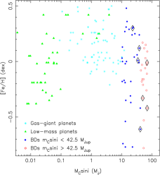
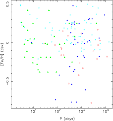
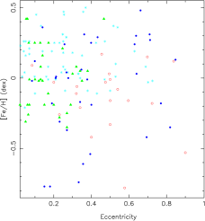
Figure 7: Stellar metallicity as a function of the brown dwarf or planetary companion properties. Colours and symbols are like in previous figures. Diamonds indicate brown dwarfs with “true” masses determinations. Left: minimum mass; Middle: period; Right: eccentricity.

Figure 8 shows the cumulative distribution function of periods (left) and eccentricities (right) for SWBDs according to the mass of the companion. The analysis of the periods reveals that for periods shorter than $\sim$ 1000 days, the sample of SWBDs with M_C$\sin i$ $>$ 42.5 M_Jup shows shorter values than SWBDs with less massive companions. A K-S test gives a probability of both samples showing the same period distribution of $\sim$ 6%. The sample of SWBDs with companions more massive than 42.5 M_Jup clearly shows higher eccentricities than the SWBDs with companions below 42.5 M_Jup, at least up to a value of $\sim$ 0.6. The K-S test on the eccentricity values suggets that both samples are statistically different ($p$-value $\sim$ 10^-16). These results are consistent with the findings of Ma & Ge (2014).

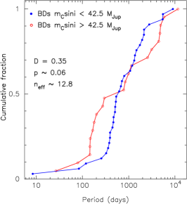
Figure 8: Cumulative distribution function of periods (left) and eccentricities (right) for SWBDs with M_C$\sin i$ $<$ 42.5 M_Jup and M_C$\sin i$ $>$ 42.5 M_Jup.

4 Discussion

The existence of the brown dwarf desert has lead to numerous theories about whether brown dwarfs form like low-mass stars, like giant-planets or by entirely different mechanisms (see e.g. Chabrier et al., 2014, for a recent review). The first observational results of this work suggests that BDs should form in a different way from gas-giant planets (if metallicity as often assumed traces the formation mechanism), as it is clear from Figure 4 that SWBDs do not follow the well-known gas-giant planet metallicity correlation. This can also be seen in the left panel of Figure 7.

In a recent work, Ma & Ge (2014) show that massive and low-mass brown dwarfs have significantly different eccentricity distributions. This difference is also seen in our sample. In particular, the authors note that BD with masses above 42.5 M_Jup have an eccentricity distribution consistent with that of binaries. This result alone could be interesting in revealing clues regarding the formation mechanism of brown dwarfs. However, based alone on the eccentricity distribution we cannot directly infer that BDs and low mass stars are formed from the same process, i.e fragmentation of a molecular cloud. Different formation mechanisms can lead to similar eccentricity distributions when subject to particular dynamical histories. What adds support to the hypothesis of a similar formation process is the fact that in our analysis we do not find any hint of metal enrichment in the stars with brown dwarf companions with masses above 42.5 M_Jup. Moreover, in all the analysis performed in this work SWBDs with masses above 42.5 M_Jup follow similar distributions to those of SWOPs or SWLMPs (see Figures 4, and  6), suggesting a non-metallicity/abundance dependent formation.

It has been shown (Stamatellos & Whitworth, 2009) that BDs can be formed via gravitational instability in the outer parts ($>$ 100 au) of massive circumstellar discs (with stellar/disc mass ratios of the order of unity). The eccentricies were found to be very high as a result of this formation process but noted that just might be an artifact of the simulations that do not include tidal interactions with the gas disc. BDs in the so-called ejection scenario are formed by gravoturbulent fragmentation of collapsing pre-stellar cores that due to dynamical interactions end-up being ejected from the cloud, terminating the accretion process (see i.e. Bate, 2009a, b). In this later scenario eccentries are not expected to populate the high end of the eccentricity distribution.

Support for a different formation mechanism for low-mass and massive brown dwarfs came from the chemical analysis performed in this work. Our results show a tendency of SWBDs with masses below 42.5 M_Jup of having slightly larger metallicities and abundances (especially X_Fe) when compared with SWBDs with masses above 42.5 M_Jup (see Figures 4,  5, and  6) although with “low” statistical significance (Table 7) We should note, however, that the results for X_Fe are statistically significant. These results can be compared with the recent work by Mata Sánchez et al. (2014), where the authors already noticed the possible higher $\alpha$-element and Fe-peak abundances in the stars hosting brown dwarfs with masses below 42.5M _Jup (in comparison with those hosting more massive brown dwarfs), however these authors do not directly test the significance of these possible trends. Furthermore, their sample of SWBDs is significantly smaller than the one analysed in this work.

If low-mass brown dwarfs were formed by core-accretion rather by the gravitational instability mechanism, stars hosting low-mass brown dwarfs should show the metal-rich signature seen in gas-giant planetary hosts (e.g. Gonzalez, 1997; Santos et al., 2004; Fischer & Valenti, 2005). It is clear from Figure 4, that SWBDs with masses below 42.5 M_Jup show lower metallicities than SWGPs. A K-S test confirms that both samples are different ($D$ $\sim$ 0.33, $p$-value $\sim$ 0.03, n_eff $\sim$ 18.5). Only for metallicities above $\sim$ +0.20 dex, the metallicity distribution of SWBDs with masses below 42.5 M_Jup approaches the distribution of the SWGP sample. As already discussed, this might be affected by the presence of additional planetary companions in some SWBDs. Indeed, when the stars with additional planets are removed from the SWBD sample, the higher metallicities of SWGPs becomes more significant ($D$ $\sim$ 0.40, $p$-value $\sim$ 0.007, n_eff $\sim$ 16.7).

Low-mass brown dwarfs might form in self-gravitating protostellar discs (Rice et al., 2003b), a fast mechanism that does not requiere the previous formation of a rocky core and therefore it is independent of the stellar metallicity (Boss, 2002, 2006). The simulations by Rice et al. (2003b) shows that the fragmentation of an unstable protostellar disc produce a large number of substellar objects, although most of them are ejected from the system. The remaining objects are typically either a very massive planet or a low-mass brown dwarf, having large periods and eccentricities. It is possible, that four of the systems discussed in Section 3.1.1 (namely HD 38529, HD 168443, HIP 5158, and HAT-P-13) with a planet in an inner orbit and a brown dwarf at a larger distance formed in this way, as well as the two brown dwarf system around the metal-poor star BD+20 2457 ([Fe/H]=-0.77 dex). The case of the system around HD 202206 (also mentioned in Section 3.1.1) might need further discussion as the brown dwarf has an inner orbit to the planet one.

Rice et al. (2003a) also shows that as the disc masses increases various effects might act to make the disc more unstable. A relationship between the disc mass and the stellar mass of the form M_disc $\propto$ M${}_{\star}^{1.2}$ were suggested (Alibert et al., 2011) to explain the observed correlation between mass-accretion rate scales and stellar mass in young low-mass objects (Muzerolle et al., 2003; Natta et al., 2004; Mendigutía et al., 2011, 2012). The fact that more massive stars might have more massive and more unstable discs might explain the presence of a relatively large number of low-mass BDs around evolved (subgiant and red giant) stars as shown that those are indeed more massive stars (e.g. Maldonado et al., 2013).

So our results on the chemical analysis of BDs suggest that at low metallicities the dominant mechanism of BD formation is compatible with gravitational instability in massive discs or gravoturbulent fragmentation of collapsing pre-stellar cores (i.e. physical mechanisms that are not depend on the metal content of the cloud). The fact that we observed differences in the metal content for low and high mass BDs at high metallicities could indicate different mechanisms operating at different efficiencies. Core accretion might favor the formation of low-mass BDs at high metallicities even at low disc masses while inhibiting the formation of massive BDs as not enough mass reservoir is available in the disc. For low-mass BDs orbiting high-metallicity host stars the core acretion model might become efficient and favor the formation of BDs even at lower disc masses and inhibit the formation of BDs with larger masses (not enough mass in the disc). It is important to note that different BD/planet formation mechanisms can operate together and do not have to be exclusive of each other.

5 Conclusions

In this work, a detailed chemical analysis of a large sample of stars with brown dwarfs has been presented. The sample has been analysed taking into account the presence of massive (M_C$\sin i$ $>$ 42.5 M_Jup) and low-mass brown dwarfs (M_C$\sin i$ $<$ 42.5 M_Jup) companions. Before comparing both subsamples, a detailed analysis of their stellar properties was performed to control any possible bias affecting our results. The chemical abundances of the SWBDs have also been compared to those of stars with known planetary companions as well as with a sample of stars without planets.

Our results show that SWBDs do not follow the well-known gas-giant metallicity correlation seen in main-sequence stars with planets. A tendency of SWBDs with substellar companions in the mass range M_C$\sin i$ $>$ 42.5 M_Jup of having slightly larger metallicities and abundances than those of SWBDs with substellar companions in the mass range M_C$\sin i$ $<$ 42.5 M_Jup seems to be present in the data. However its statistical significancy is rather low. We also confirm possible differences between SWBDs with substellar companions with masses above and below 42.5 M_Jup in terms of periods and eccentricities. All this observational evidence suggests that the efficiencies of the different formation mechanisms may differ for low-mass and high-mass brown dwarfs.

Our results are well described in a scenario in which high-mass brown dwarfs are mainly formed like low-mass stars (by the fragmention of a molecular cloud). Our analysis shows that at high metallicities the core-accretion model might be the mechanism for the formation of low-mass BDs. On the other hand, it seems reasonable that the most suitable scenario for the formation of low-metallicity, low-mass BDs is gravitational instability in turbulent protostellar discs since this mechanism is known to be independent of the stellar metallicity.