Neutron star crusts from mean field models constrained
by chiral effective field theory

Abstract

We investigate the structure of neutron star crusts, including the crust-core boundary, based on new Skyrme mean field models constrained by the bulk-matter equation of state from chiral effective field theory and the ground-state energies of doubly-magic nuclei. Nuclear pasta phases are studied using both the liquid drop model as well as the Thomas-Fermi approximation. We compare the energy per nucleon for each geometry (spherical nuclei, cylindrical nuclei, nuclear slabs, cylindrical holes, and spherical holes) to obtain the ground state phase as a function of density. We find that the size of the Wigner-Seitz cell depends strongly on the model parameters, especially the coefficients of the density gradient interaction terms. We employ also the thermodynamic instability method to check the validity of the numerical solutions based on energy comparisons.

I Introduction

Neutron stars offer the possibility to study matter under extreme conditions (in density and neutron-to-proton ratio) inaccessible to laboratory experiments on Earth. The inner core of a neutron star may reach densities as high as five to ten times nuclear saturation density, a regime for which no well-converged theoretical expansions are presently available. The structure and composition of the inner core is consequently highly uncertain and may contain deconfined quark matter Weber (2005); Alford et al. (2005); Weissenborn et al. (2011), hyperonic matter Schaffner-Bielich et al. (2002); Weissenborn et al. (2012a, b); Lim et al. (2015); Chatterjee and Vidaña (2016), or meson condensates Baym (1973); Thorsson et al. (1994); Glendenning and Schaffner-Bielich (1998); Lim et al. (2014). In contrast, the inner crust and outer core span densities from $n\simeq 4\times 10^{11}-5\times 10^{14}$ g/cm³, corresponding to nucleon Fermi momenta of $k_{F}\lesssim 400$ MeV, which is much less than the chiral symmetry breaking scale of $\Lambda_{\chi}=4\pi f_{\pi}\simeq 1$ GeV. Chiral effective field theory (EFT) Weinberg (1979) may therefore provide a suitable theoretical framework for exploring neutron star matter at these densities.

In recent years there has been significant progress in the development of realistic chiral nucleon-nucleon (NN) forces Epelbaum et al. (2009a); Machleidt and Entem (2011); Epelbaum et al. (2015); Entem et al. (2015) at and beyond next-to-next-to-next-to-leading order (N3LO) in the chiral power counting. Nuclear many-body forces become relevant in homogeneous matter at densities larger than $n\gtrsim 0.25n_{0}$ (where $n_{0}=2.4\times 10^{14}$ g/cm³ is the saturation density of nuclear matter) and have been included in numerous studies of the cold nuclear and neutron matter equations of state (EOS) Epelbaum et al. (2009b); Hebeler and Schwenk (2010); Hebeler et al. (2011); Coraggio et al. (2013); Gezerlis et al. (2013); Tews et al. (2013); Coraggio et al. (2014); Roggero et al. (2014); Wlazłowski et al. (2014); Carbone et al. (2014); Tews et al. (2016). Neutron star structure and evolution requires in addition the equation of state at arbitrary isospin-asymmetry Drischler et al. (2014); Wellenhofer et al. (2016) and finite temperature Tolos et al. (2008); Wellenhofer et al. (2014, 2015), which has been computed consistently with the same chiral nuclear force models and many-body methods. The inhomogeneous phase of nuclear matter encountered in neutron star crusts depends also on gradient contributions to the energy density. Previous work has focused on the leading-order Hartree-Fock contribution to the isoscalar and isovector gradient couplings from the density matrix expansion Bogner et al. (2009); Holt et al. (2011); Kaiser (2012), ab initio studies of the isovector gradient coupling strength from quantum Monte Carlo simulations of pure neutron matter Gandolfi et al. (2011); Buraczynski and Gezerlis (2016a), and nuclear response functions in Fermi liquid theory Lykasov et al. (2008); Davesne et al. (2015); Holt et al. (2012, 2013a).

Neutron star crusts have been studied using phenomenological liquid drop models Ravenhall et al. (1983a); Douchin and Haensel (2001); Newton et al. (2013) and the Thomas-Fermi approximation Oyamatsu (1993); Okamoto et al. (2013). Nuclear pasta phases resulting from the competition between the Coulomb interaction and nuclear surface tension were also treated in the liquid drop and Thomas-Fermi methods. More sophisticated approaches to the nuclear pasta phase have been investigated using the Skyrme-Hartree Fock approximation Newton and Stone (2009); Pais and Stone (2012); Schuetrumpf and Nazarewicz (2015) and molecular dynamic simulations Horowitz et al. (2005); Sonoda et al. (2008); Schneider et al. (2013).

In the present work we utilize recent results for the homogeneous nuclear matter equation of state from chiral EFT to develop new Skyrme mean field parametrizations that enable the study of finite nuclei, inhomogeneous nuclear matter in neutron star crusts, and the mass-radius relation of neutron stars. Recent works Brown and Schwenk (2014); Bulgac et al. (2015); Rrapaj et al. (2016) have used the low-density equation of state of neutron matter from chiral EFT to constrain nonrelativistic and relativistic mean field models, while the present study includes the full isospin-asymmetric matter equation of state at second order in perturbation theory up to $n=2n_{0}$ as a fitting constraint. Several chiral nuclear force models are considered in order to estimate the theoretical uncertainty.

We find that the traditional Skyrme model cannot accommodate the density dependence of the nuclear equations of state derived from chiral effective field theory. We therefore introduce additional interaction terms in the Skyrme Hamiltonian that go as the next higher power of the Fermi momentum. This enables an accurate reproduction of the bulk-matter equation of state from chiral EFT. Using the new models, we investigate the phase of sub-saturation nuclear matter, which is expected to be present at the boundary between the outer core and inner crust of neutron stars, an environment that is highly neutron rich. Indeed the proton fraction of nuclear matter in beta equilibrium at the crust-core boundary is roughly $\sim 3\%$. In the boundary region, nuclear matter experiences a shape change caused by the competition between the repulsive Coulomb interaction and surface tension. We adopt the analytic solution of the Coulomb interaction in discrete dimensions to study the phase of nuclear matter in the liquid drop model (LDM) formalism. The energy per nucleon of nuclear matter determines the lowest energy state and therefore the discrete shape in the pasta phase. We also study inhomogeneous nuclear matter by employing the Thomas-Fermi (TF) approximation employing a parameterized density profile (PDP) for neutrons and protons.

The paper is organized as follows. In Section II we describe the Skyrme force model used to investigate the neutron star inner crust and outer core. The traditional Skyrme model is extended in order to reproduce the homogeneous matter equation of state of isospin-asymmetric nuclear matter from chiral effective field theory as well as the ground state energies of doubly magic nuclei. In Section III, we present the numerical method to determine the transition density for the core-crust boundary. The liquid drop model, Thomas-Fermi approximation, and thermodynamic instability methods are then employed to find the transition densities. We summarize our results in Section IV.

II Nuclear Model

We begin by describing the microscopic chiral nuclear force models Entem and Machleidt (2003); Coraggio et al. (2014) employed in the present study. The two-body force is treated at N3LO in the chiral expansion, and the 24 low-energy constants associated with NN contact terms are fitted to elastic nucleon-nucleon scattering phase shifts and deuteron properties. The three-body force is treated at N2LO, and the $c_{E}$ and $c_{D}$ low-energy constants associated with the contact three-body force and one-pion exchange three-body force, respectively, are fitted to reproduce the ground-state energies of ³H and ³He as well as the beta-decay lifetime of ³H. The resolution scale is set by the momentum-space cutoff $\Lambda$, which is varied over the range $414\,{\rm MeV}<\Lambda<500$ MeV. At this resolution scale many-body perturbation theory is well converged, and the resulting neutron matter equation of state below saturation density is strongly constrained Holt and Kaiser (2016). Cutoff variation provides only one means to study the theoretical uncertainties in chiral effective field theory, and future work will be devoted understanding better the errors due to neglected higher-order terms in the chiral expansion.

To be specific we use three different values of the momentum-space cutoff $\Lambda=414$, $450$, $500$ MeV and denote the corresponding nuclear potentials as n3lo414, n3lo450, and n3lo500. The strategy is then to identify what approximations are needed in each case to provide an accurate description of the bulk matter equation of state in the vicinity of nuclear matter saturation. As shown in previous work Coraggio et al. (2014), the chiral potentials with the two lowest cutoff values give reasonable nuclear matter properties at second-order in many-body perturbation theory with Hartree-Fock intermediate-state propagators. In particular, the saturation energy lies in the range $E/A=-(15.7-16.2)$ MeV while the saturation density lies in the range $n_{0}=(0.165-0.174)$ fm^-3. At the same approximation in many-body perturbation theory, the $\Lambda=500$ MeV chiral potential exhibits too little attraction, and the binding energy per nucleon at saturation density is only $E/A\simeq-11.5$ MeV. We therefore employ for this potential second-order perturbation theory with free-particle intermediate-state energies, which on the one hand accounts for theory uncertainties associated with the choice of the single-particle energy spectrum and on the other hand leads to an improved description of nuclear matter saturation. The latter results from a larger density of states near the Fermi surface that enhances the overall attraction from the second-order perturbative contribution. In this case the saturation energy and density are $E/A=-15.9$ MeV and $n_{0}=0.171$ fm^-3, respectively.

The calculations outlined above have been extended in the present work to describe cold nuclear matter at arbitrary isospin asymmetry. The resulting equations of state are then used as data in fitting new Skyrme model parametrizations. In addition, the density-gradient contributions to the nuclear energy density, which have important effects on the structure of the neutron star inner crust, are constrained by including the ground-state energies of doubly-magic nuclei in the $\chi^{2}$ minimization function for the Skyrme model parameters.

The same two- and three-body chiral potentials have also been used in numerous studies of nuclear dynamics and thermodynamics (for recent reviews, see Refs. Holt et al. (2013b, 2016). In particular, the critical endpoint of the first-order liquid-gas phase transition line was found Wellenhofer et al. (2014) to be consistent with recent empirical determinations Elliott et al. (2013), and the low-density–high-temperature equation of state of pure neutron matter was found Wellenhofer et al. (2015) to be in very good agreement with the model-independent virial expansion. The applications described below focus on the cold neutron star composition and equation of state, but we may anticipate future extensions to finite temperature matter employing a strategy similar to that described above.

The energy density in dense nuclear matter can be expanded in powers of the proton and neutron Fermi momenta, $k_{f}^{p}=(3\pi^{2}n_{p})^{1/3}$ and $k_{f}^{n}=(3\pi^{2}n_{n})^{1/3}$, as follows

$$\varepsilon= \frac{\hbar^{2}}{2m}(\tau_{n}+\tau_{p})+\alpha_{L}(n_{n}^{2}+n_{p}^{2})+2\alpha_{U}n_{n}n_{p}$$ (1)

$$+\left[\eta_{L}(n_{n}^{2}+n_{p}^{2})+2\eta_{U}n_{n}n_{p}\right]n^{\gamma}\,,$$

where

$$\tau_{n}= \frac{3}{5}(3\pi^{2})^{2/3}n^{5/3}(1-x)^{5/3},$$ (2)

$$\tau_{p}= \frac{3}{5}(3\pi^{2})^{2/3}n^{5/3}(1-x)^{5/3},$$

$n_{n}=n(1-x)$, and $n_{p}=nx$. The above approximation can explain $\chi$EFT asymmetric matter results quite well with small deviation ($<1\%$), at least for $T=0$ MeV. However, it cannot be used to calculate the properties of finite nuclei directly unless we find the surface tension in the liquid drop model or the gradient terms in the Thomas-Fermi approximation

The polynomial expansion in Eq. (1) can be derived from the phenomenological Skyrme nucleon-nucleon interaction, given by

$$v_{i,j} ({\mathbf{r}}_{i},{\mathbf{r}}_{j})=t_{0}(1+x_{0}P_{\mathbf{\sigma}})\delta(\mathbf{r}_{i}-\mathbf{r}_{j})$$ (3)

$$+\frac{t_{1}}{2}(1+x_{1}P_{\mathbf{\sigma}})\Bigl{[}\delta(\mathbf{r}_{i}-\mathbf{r}_{j})\mathbf{k}^{2}+\mathbf{k}^{\prime 2}\delta(\mathbf{r}_{i}-\mathbf{r}_{j})\Bigr{]}$$

$$+t_{2}(1+x_{2}P_{\mathbf{\sigma}})\mathbf{k}^{\prime}\cdot\delta(\mathbf{r}_{i}-\mathbf{r}_{j})\mathbf{k}$$

$$+\frac{1}{6}t_{3}(1+x_{3}P_{\mathbf{\sigma}})\rho^{\alpha}\delta(\mathbf{r}_{i}-\mathbf{r}_{j})$$

$$+iW_{0}\mathbf{k}^{\prime}\delta(\mathbf{r}_{i}-\mathbf{r}_{j})\times\mathbf{k}\cdot(\bm{\sigma}_{i}+\bm{\sigma}_{j})\,,$$

where $P_{\sigma}$ is the spin exchange operator, the local density $\rho$ is evaluated at $(\mathbf{r}_{i}+\mathbf{r}_{j})/2$, $\mathbf{k}=\frac{1}{2i}(\nabla_{i}-\nabla_{j})$, and $\mathbf{k}^{\prime}=-\frac{1}{2i}(\nabla^{\prime}_{i}-\nabla^{\prime}_{j})$.

Table 1: Skyrme force parameters fitted to the chiral N3LO asymmetric matter equation of state and finite nuclei binding energies. The parameters have units such that the energy density is given in MeV fm^-3.

	Sk$\chi$414	Sk$\chi$450	Sk$\chi$500
$t_{0}$	$-1734.0261$	$-1803.2928$	$-1747.48258$
$t_{1}$	$255.6550$	$301.8208$	$241.31968$
$t_{2}$	$-264.0678$	$-273.2827$	$-331.04118$
$t_{3}$	$12219.5884$	$12783.8619$	$12491.50533$
$t_{4}$	$556.1320$	$564.1049$	$405.03174$
$x_{0}$	$0.4679$	$0.4430$	$0.59530$
$x_{1}$	$-0.5756$	$-0.3622$	$-1.15893$
$x_{2}$	$-0.3955$	$-0.4105$	$-0.58432$
$x_{3}$	$0.7687$	$0.6545$	$1.20050$
$x_{4}$	$-15.8761$	$-11.3160$	$-25.49381$
$\gamma_{1}$	$1/3$	$1/3$	$1/3$
$\gamma_{2}$	$1$	$1$	$1$
$W_{0}$	$93.7236$	$106.4288$	$98.08897$

Traditional Skyrme force models have 10 parameters which can be fitted to the binding energies of finite nuclei, neutron skin thicknesses, bulk matter properties, and neutron matter calculations. However, we find that this number of parameters is insufficient to reflect both the equation of state of asymmetric nuclear matter from chiral EFT as well as the properties of finite nuclei. We therefore extend the traditional Skyrme force model by adding extra density dependent terms of the form

$$v_{ij}\rightarrow v_{ij}+\frac{1}{6}t_{4}(1+x_{4}P_{\sigma})\rho^{\gamma_{2}}\delta(\mathbf{r}_{i}-\mathbf{r}_{j})\,.$$ (4)

We determine the Skyrme Hartree-Fock parameters from fitting to the recent $\chi$EFT asymmetric nuclear matter calculations outlined in Ref. Wellenhofer et al. (2016) together with the binding energies of doubly closed shell nuclei. We define the $\chi^{2}$ minimization function:

$$\chi^{2}(x_{0},\dots,x_{4},t_{0},\dots,t_{4},W_{0})$$ (5)

$$\quad=w_{b}\left[\frac{1}{N_{i}N_{j}}\sum\left\{\frac{\mathcal{E}^{\mathrm{EFT}}(n_{i},x_{j})-\mathcal{E}^{\mathrm{Sk}}(n_{i},x_{j})}{\mathrm{MeV}}\right\}^{2}\right]$$

$$\quad+w_{n_{0}}(0.16-\rho_{0}~{}\mathrm{fm}^{3})^{2}+w_{B}(-16+B^{\mathrm{Sk}}~{}\mathrm{MeV}^{-1})^{2}$$

$$\quad+w_{F}\left[\frac{1}{N_{k}}\sum\left(\frac{B_{k}^{\mathrm{Exp.}}-B_{k}^{\mathrm{Sk}}}{\mathrm{MeV}}\right)^{2}\right]\,$$

with weighting factors {$w_{b}$, $w_{n_{0}}$, $w_{B}$, $w_{F}$}.

Since Hartree-Fock theory is the lowest order approximation in a systematic many-body perturbation theory expansion, there is no clean one-to-one correspondence between the Skyrme parameters and the chiral expansion coefficients. It is, however, possible to reproduce properties of the chiral EFT equation of state from a simplified Skyrme mean field model. The desirable aspect of the Skyrme parametrization is that it enable us to then calculate also the properties of finite nuclei, such as their density profiles and binding energies, as well as the composition and structure of neutron star inner crusts.

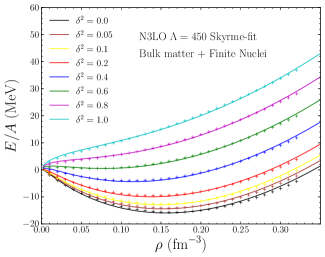
Figure 1: (Color online) Comparison of the energy per baryon in asymmetric nuclear matter from chiral EFT ($\Lambda=450$ MeV) and its Skyrme fitting model. The isospin asymmetry is denoted by $\delta=(n_{n}-n_{p})/(n_{n}+n_{p})$.

We present the new Skyrme parametrizations in Table 1. We set $\gamma_{1}=1/3$ and $\gamma_{2}=1$ in all cases. This can be justified when we consider that the energy density of bulk nuclear matter can be expanded as a function of the Fermi momentum $k_{f}$. Note that $x_{4}$ is much larger than the other $x$’s in the parametrization. This indicates that spin exchange interactions give very large attraction in dense matter within the extended Skyrme formalism. Figure 1 shows the energy per baryon in asymmetric nuclear matter from both chiral effective field theory and Skyrme phenomenology. The ‘$+$’ denotes the energy per baryon from $\chi$EFT with $\Lambda=450$ MeV, while the solid lines are results from the new Skyrme models derived in our work. The deviations get larger as the total baryon number density increases, but overall the agreement is quite satisfactory given the simplicity of the Skyrme mean field model. We have performed the same fitting procedure also for the $\Lambda=414$ MeV and $\Lambda=500$ MeV chiral nuclear potentials, and in these cases the fit is of the same quality as that shown in Fig. 1 for the case $\Lambda=450$ MeV. We include as well the total binding energy of doubly magic nuclei in the $\chi^{2}$ minimization function for the Skyrme parametrizations. Table 2 shows the results of the Skyrme Hartree-Fock calculations compared to the experimental values Audi et al. (2015).

Table 2: Skyrme Hartree-Fock results for the binding energies (in units of MeV) of doubly closed shell nuclei together with bulk nuclear matter properties Dutra et al. (2012).

	Exp.	Sk$\chi$414	Sk$\chi$450	Sk$\chi$500
16O	127.62	126.73	126.93	127.07
40Ca	342.05	342.63	341.93	341.43
48Ca	415.99	416.66	416.69	417.24
56Ni	483.99	482.29	482.32	482.38
100Sn	825.78	826.20	825.69	822.55
132Sn	1102.90	1103.05	1103.22	1106.91
208Pb	1636.44	1635.88	1636.21	1635.30
$\rho_{0}$ ($\mathrm{fm}^{-3}$)	$0.160\pm 0.005$	0.1697	0.1562	0.1679
$B$ (MeV)	$16.0\pm 0.5$	16.1987	15.9262	15.9895
$K$ (MeV)	$230\pm 30$	243.19	239.53	238.16
$S_{v}$ (MeV)	$32.5\pm 2.5$	32.3456	30.6346	29.1167
$L$ (MeV)	$58\pm 18$	51.9307	42.0518	40.7415

Having determined all Skyrme model parameters from the $\chi^{2}$ fitting function in Eq. (5), we now check theoretical predictions for bulk matter and finite nuclei. Also in Table 2 we show the properties of nuclear matter around the saturation density, including the saturation energy per particle $B$, the nuclear incompressibility $K$, the isospin-asymmetry energy $S_{v}$, and the isospin-asymmetry slope parameter $L$. Overall the microscopic predictions agree very favorably with experimental constraints Dutra et al. (2012).

As an example of the Skyrme Hartree-Fock calculations for finite nuclei, we present the density profile of ²⁰⁸Pb in Fig. 2. The experimental charge density De Vries et al. (1987) is included for comparison.

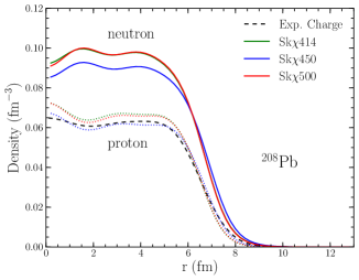
Figure 2: (Color online) Density profile of neutron and proton in ²⁰⁸Pb using Skyrme Hartree Fock. Experimental charge density is also added for comparison.

The central density of ²⁰⁸Pb from the $\Lambda=414$ MeV and $\Lambda=500$ MeV chiral potentials is greater than that from the $\Lambda=450$ MeV potential model. This can be understood by noting that the saturation density of the $\Lambda=450$ MeV model is close to the empirical value of $n_{0}=0.16$ fm^-3, while the other two potentials give saturation densities closer to $n_{0}=0.17$ fm^-3.

To check the behavior of the Skyrme mean field models in the high-density region ($\rho>0.4\mathrm{\,fm}^{-3}$), we solve Tolman-Oppenheimer-Volkov (TOV) equations for a static cold neutron star:

$$\frac{dp}{dr} =-\frac{G(M(r)+4\pi r^{3}p)(\varepsilon+p)}{r(r-2GM(r))},$$ (6)

$$\frac{dM}{dr} =4\pi\varepsilon r^{2},$$

where $r$ is the radial distance from the center, $M(r)$ is the enclosed mass of a neutron star within $r$, $\varepsilon$ represents the energy density and $p$ the pressure. Figure 3 shows the mass and radius curves for the three different Skyrme parameter sets. The central shaded area is a comprehensive estimate of neutron star radii from observations of X-ray bursters Steiner et al. (2010). The rectangular bars around $2.0M_{\odot}$ represent observational constraints on the maximum neutron star mass Demorest et al. (2010); Antoniadis et al. (2013). For all three Skyrme parametrizations we see that the maximum neutron star mass is equal to $2.1M_{\odot}$. Therefore, all of the parameter sets satisfy the maximum mass constraint and moreover are also consistent with the radius constraint.

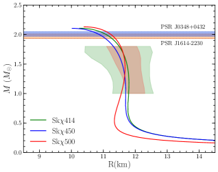
Figure 3: (Color online) Mass-radius curves from the Skyrme mean field models constructed in the present work.

III Core-Crust Boundary

III.1 Asymmetric matter equation of state and nuclear mass tables

To orient the discussion of the neutron star crust-core transition, we begin with a simple model of the crust derived from the BBP Baym et al. (1971) formalism. Here the nuclear mass table is used to determine the energy per nucleon in the crust. When combined with the beta-equilibrium equation of state for homogeneous nuclear matter, it is possible to estimate the crust-core transition density. In the BBP formalism, a single nucleus stays at the center of a spherical unit cell called the “Wigner-Seitz Cell” along with a gas of unbound electrons and neutrons. The total energy density is then given by

$$\varepsilon=n_{N}M(A,Z)+n_{N}W_{L}+\varepsilon_{n}(n_{n})(1-V_{N}n_{N})+\varepsilon_{e}(n_{e})\,,$$ (7)

where $n_{N}$ is the number density of heavy nuclei with $A$ nucleons ($Z$ protons), $V_{N}$ is the volume of a nucleus so that $(1-V_{N}n_{N})$ is the volume fraction given to neutrons in the Wigner-Seitz cell, $W_{L}$ is the lattice energy arising from the interaction between electrons and protons in the unit cell, and $n_{n}$ and $n_{e}$ are the number densities of unbound neutrons and electrons in the cell. The energy density of neutrons $\varepsilon_{n}$ is taken from the zero-temperature neutron matter equation of state from chiral EFT, while the electron energy density $\varepsilon_{e}$ is given by

$$\varepsilon_{e}=\frac{m_{e}^{4}}{8\pi^{2}}\left[x\sqrt{1+x^{2}}(1+2x^{2})-\ln(x+\sqrt{1+x^{2}})\right]\,,$$ (8)

where $x=k_{F}^{e}/m_{e}$ is the electron Fermi momentum divided by its mass.

Since the Skyrme Hartree-Fock nuclear masses contain the Coulomb energy for proton-proton interactions, it is necessary to subtract the Coulomb energy when computing the lattice energy. In this work, we consider the exchange Coulomb energy from electrons. Thus the total Coulomb lattice energy from electrons and protons is given by

$$W_{L+C}^{\prime}= \frac{3}{5}\frac{Z^{2}e^{2}}{r_{N}}\left[\left(1-\frac{r_{N}}{r_{c}}\right)^{2}\left(1+\frac{r_{N}}{2r_{c}}\right)-1\right]$$ (9)

$$-\frac{3e^{2}}{4}\left(\frac{3}{\pi}\right)^{1/3}\frac{n_{e}^{4/3}}{n_{N}}$$

$$= \frac{3}{10}\frac{Z^{2}e^{2}}{r_{o}A^{1/3}}(u-3u^{1/3})-\frac{3}{4}\frac{Z^{4/3}e^{2}}{r_{o}A^{1/3}}\left(\frac{3}{2\pi}\right)^{2/3}u^{1/3},$$

where $u$ is the volume fraction of the nucleus in the Wigner-Seitz cell, i.e., $V_{c}=\frac{4\pi}{3}r_{c}^{3}=1/n_{N}$ and $u=V_{N}/V_{c}$. The radius of a heavy nucleus in the unit cell is given by $r_{N}=r_{o}A^{1/3}$, where $n_{0}=(\frac{4\pi}{3}r_{o}^{3})^{-1}=0.16~{}\mathrm{fm}^{-3}$. Heavy nuclei are therefore assumed to be of uniform density $n_{0}$.

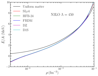
Figure 4: (Color online) Energy per nucleon in the neutron star crust for each mass model together with the n3lo450 beta-equilibrium bulk matter calculation.

The approach outlined above gives us a first estimate for the transition density between inhomogeneous nuclear matter in the neutron star crust and uniform neutron matter in the core. The transition to homogeneous matter occurs when the energy density of the Wigner-Seitz cell containing a heavy nucleus becomes larger than that of homogeneous nuclear matter in beta-equilibrium. In Fig. 4 we show the energy per baryon in the neutron star crust using various nuclear mass models together with the bulk matter equation of state (we take as a representative example that from the n3lo450 chiral nuclear potential). All of the nuclear mass models give very similar finite nuclei binding energies, but slight differences give rise to crust-core transition densities in the range $0.035<\rho_{t}<0.052$ fm^-3.

In Table 3 we show the transition densities using various nuclear mass models together with the three neutron matter equations of state described in Section II. Note that the Gogny D1S mass model consistently gives the lowest transition density, which is related to the relatively fast approach to neutron drip in the model. We observe that the uncertainty in the transition density coming from the choice of nuclear mass model is much larger than that from the choice of the bulk matter equation of state. This is due to the fact that at these relatively low values for the transition density, the chiral effective field theory expansion of the nuclear equation of state is well converged Holt and Kaiser (2016).

Overall, the use of a nuclear mass table together with the bulk matter equation of state is a rather crude method to obtain the neutron star crust-core phase boundary. We will show in more detail below that the model predicts a transition density that is too small, since each mass table only accounts for the possibility of neutron-rich nuclei in the Wigner-Seitz cell for which the neutron chemical potential is less than zero. In the inner crust of neutron stars, the neutron chemical potential is greater than zero as neutrons drip out of heavy nuclei to form the free gas of neutrons. Thus, the mass information of finite nuclei is only useful to describe the neutron star outer crust Ruester et al. (2006).

Table 3: The core-crust transition densities in units of fm^-3 from various nuclear model combinations. References are for the finite nuclei calculations.

Model	Sk$\chi$414	Sk$\chi$450	Sk$\chi$500	Ref.
SLy4	0.03562	0.03556	0.03481	Stoitsov et al. (2003)
HFB-24	0.04256	0.04291	0.04025	Goriely et al. (2013)
FRDM	0.05140	0.05196	0.04612	Moller et al. (2016)
DZ	0.04471	0.04512	0.04172	Duflo and Zuker (1995)
D1S	0.03505	0.03524	0.03436	Hilaire and Girod (2007)

III.2 Compressible Liquid Drop Model

A more realistic approach to study the neutron star inner crust equation of state is to utilize the liquid drop model (LDM) in the Wigner-Seitz cell approximation. The energy density used to obtain the ground state of inhomogeneous nuclear matter in the crust of a neutron star can be written as

$$\varepsilon =un_{i}f_{i}+\frac{\sigma(x_{i})ud}{r_{N}}+2\pi(n_{i}x_{i}er_{N})^{2}uf_{d}(u)$$ (10)

$$+(1-u)n_{no}f_{no}\,,$$

where $u$ is the filling factor (the fraction of space taken up by a heavy nucleus in the Wigner-Seitz cell), $n_{i}$ is the number density of heavy nuclei, $x_{i}$ is the proton fraction, $f_{i}$ represents the volume contribution to the energy per baryon in the heavy nucleus obtained from the new Skyrme parametrizations, $\sigma(x_{i})$ is the surface tension as a function of the proton fraction, $r_{N}$ is the heavy nucleus radius, $n_{no}$ is the density of the unbound neutron gas, $f_{no}$ is the energy density of the neutron gas, and $f_{d}$ is a geometric function describing the Coulomb interaction Ravenhall et al. (1983a) for different dimensions $d$. The surface tension is given explicitly by

$$\sigma(x)=\sigma_{0}\frac{2^{\alpha+1}+q}{(1-x)^{-\alpha}+q+x^{-\alpha}},$$ (11)

where $q$ parametrizes how quickly the surface tension decreases as a function of the proton fraction $x$. Larger values of $q$ correspond to more gradual decreases in the surface tension for neutron-rich nuclei. The parameterization of the surface tension in Eq. (11) avoids the problem of negative values that can occur for highly neutron-rich nuclei when a simple quadratic formula for the surface tension is used Ravenhall et al. (1983b). The numerical values of $\sigma_{0}$ and $q$ are fitted to give the lowest root-mean-square deviation to known nuclear masses. For the three chiral interactions n3lo414, n3lo450 and n3lo500, we find $\sigma_{0}=\{1.311,\,1.186,\,1.233\}$ MeV-fm^-2 and $q=\{40.362,\,46.748,\,69.413\}$, respectively. In all cases $\alpha=3.4$ is used since it is adequate in describing both isolated nuclei and nuclei in dense matter.

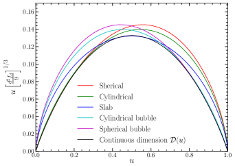
Figure 5: (Color online) Shape function $\mathcal{D}(u)$ for discrete dimension and continuous dimension. The continuous dimension curve always lies below those of the discrete geometries.

The Coulomb energies for different nuclear geometries (e.g., cylindrical or planar) are encoded in the function

$$f_{d}(u)=\frac{1}{d+2}\left[\frac{2}{d-2}\left(1-\frac{1}{2}du^{1-2/d}\right)+u\right].$$ (12)

The case $d=3$ corresponds to spherical shape, $d=2$ to cylindrical shape, and $d=1$ to slab shape. The equation for spherical bubble geometry can be obtained with the replacement $u\sigma\rightarrow(1-u)\sigma$ and $uf_{d}(u)\rightarrow(1-u)f_{d}(1-u)$. For a given baryon number density $n$ and proton fraction $Y_{p}$, we solve the following equations for the four unknowns {$u$, $n_{i}$, $x_{i}$, $n_{no}$}:

$$\mu_{ni}-\frac{x_{i}\sigma^{\prime}(x_{i})d}{r_{N}n_{i}}=\mu_{no}\,,$$ (13a)

$$P_{i}-2\pi(n_{i}x_{i}er_{N})^{2}\frac{\partial(uf_{d})}{\partial u}=P_{no}\,,$$ (13b)

$$n-un_{i}-(1-u)n_{no}=0\,,$$ (13c)

$$nY_{p}-un_{i}x_{i}=0\,,$$ (13d)

where $n$ is the total baryon number density in the Wigner-Seitz cell. From the nuclear virial theorem the surface energy $E_{S}=\sigma(x_{i})ud/r_{N}$ is related to the Coulomb energy $E_{C}=2\pi(n_{i}x_{i}er_{N})^{2}uf_{d}(u)$ by $E_{S}=2E_{C}$, which is obtained by setting $\partial\varepsilon/\partial r_{N}=0$. This gives Lattimer and Swesty (1991) the relation $E_{S}+E_{C}=\beta\mathcal{D}$, where $\beta=\left(\frac{243\pi}{2}\right)^{1/3}(n_{i}x_{i}e\sigma)^{2/3}$ and $\mathcal{D}(u)=u\left[\frac{d^{2}f_{d}}{9}\right]^{1/3}$. If we allow $d$ to be continuous, we can find the shape function $\mathcal{D}$ that describes all pasta phases with a single formula.

We adopt the function $\mathcal{D}$ used in the Lattimer-Swesty EOS Lattimer and Swesty (1991):

$$\mathcal{D}(u)=u(1-u)\frac{(1-u)f_{3}^{1/3}+uf_{3}^{1/3}(1-u)}{u^{2}+(1-u)^{2}+0.6u^{2}(1-u)^{2}}\,.$$ (14)

The combined pasta phase model can be implemented if a continuous dimension $d$ is allowed. Fig. 5 shows the shape function $\mathcal{D}(u)$ for each discrete dimension (shown as colored lines) as well as for continuous dimension (black line). The latter has the correct behavior as $u\rightarrow 0$ and $u\rightarrow 1$. It represents the energy state that minimizes the combined Coulomb and surface energies.

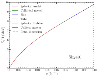
Figure 6: (Color online) Energy per nucleon as a function of baryon number density in beta-stable nuclear matter employing the liquid drop model with the Sk$\chi$450 Skyrme mean field model.

Note that the dimension of the lowest energy state will be determined by the volume fraction of dense matter in the Wigner-Seitz cell. The crossing points for each dimension are independent of the equation of state and occur at the values $u=\{0.21525,0.35499,0.64501,0.78475\}$ for the {3D-2D, 2D-1D, 1D-2DB, 2DB-3DB} transitions. For instance, if the volume fraction of dense matter is 0.4, then the lowest energy state is the slab phase.

In Fig. 6 we show the energy per baryon in the geometric configuration with the lowest energy, including also the beta-equilibrium condition. As the density increases the lowest energy state proceeds through $d=3,2,1,2b,3b,$ and finally to uniform matter. By “2b” and “3b” we denote the two-dimensional and three-dimension bubble geometries. The solution found by employing a continuous dimension correctly represents the lowest energy state.

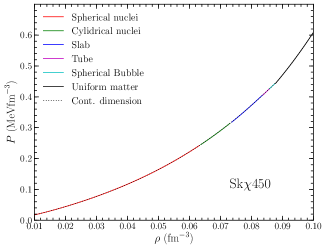
Figure 7: (Color online) Pressure as a function of baryon number density in beta-stable nuclear matter employing the liquid drop model with the Sk$\chi$450 Skyrme mean field model. At each transition density the pressure is almost continuous in the case of the LDM approach.

The first derivative of $E/A$ with respect to the baryon number density, namely the pressure, is shown in Fig. 7. The pressure at each transition density is essentially continuous in the LDM formalism. The continuous dimension LDM also gives the correct numerical values compared with the discrete dimension calculation in the LDM.

In Table 4 we show the phase transition densities to different nuclear pasta geometries in the neutron star inner crust. We see that the different Sk$\chi$ mean field models predict similar transition densities for each of the phases, with uncertainties less than $0.006$ fm^-3.

Table 4: Transition densities (in unit of fm^-3) between different geometries in the neutron star inner crust using the LDM method.

	Sk$\chi$414	Sk$\chi$450	Sk$\chi$500
3DN-2DN	0.0665	0.0634	0.0656
2DN-1DN	0.0766	0.0736	0.0782
1DN-2DB	0.0864	0.0837	0.0895
2DB-3DB	0.0884	0.0859	0.0918
3DB-Uni.	0.0901	0.0878	0.0940

In Fig. 8 we show the volume fraction of dense matter in the Wigner-Seitz cell for each discrete dimension and continuous dimension calculation. The volume fractions for the lowest energy states are in the correct regions as expected. Therefore, the volume fraction of the dense phase in the Wigner-Seitz cell at each dimension can be used to identify the ground state dimension among the different pasta phases. The continuous dimension approach provides a reliable way to construct the nuclear equation of state in the pasta phase analytically. This also indicates that the supernova EOS table Lattimer and Swesty (1991) using the continuous dimension is a valid numerical method that does not destroy the continuity in pressure at each transition density.

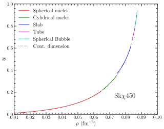
Figure 8: (Color online) Volume fraction of the dense phase in the Wigner-Seitz cell. The volume fraction indicates which dimension is the ground state for a given baryon number density.

III.3 Thomas-Fermi Approximation

In the Thomas-Fermi (TF) approximation, the number density and kinetic momentum density are given by

$$\rho_{t}=\frac{1}{4\pi^{2}}\int_{0}^{\infty}f_{t}d^{3}p\,,\quad\tau_{t}=\frac{1}{4\pi^{2}}\int_{0}^{\infty}f_{t}p^{2}d^{3}p$$ (15)

where $t$ is the type of nucleon and $f_{t}$ is the Fermi occupation function:

$$f_{t}=\frac{1}{1+\exp{\left(\frac{\varepsilon_{t}-\mu_{t}}{T}\right)}}\,,$$ (16)

where $\varepsilon_{t}$ is the single particle energy for protons or neutrons and $\mu_{t}$ is the chemical potential for each species. At $T=0$ MeV this equation simply gives $\tau_{t}=\frac{3}{5}(3\pi^{2})^{2/3}\rho_{t}^{5/3}$. In the crust of neutron stars, the density profile of inhomogeneous nuclear matter can be parametrized Oyamatsu (1993) as

$$n_{t}(r)=\begin{cases}(n_{ti}-n_{to})\left[1-\left(\frac{r}{R_{t}}\right)^{\alpha_{t}}\right]^{3}+n_{to}&\text{if}\quad r<R_{t}\,,\\ n_{to}&\text{if}\quad r\geq R_{t}\,.\end{cases}$$ (17)

When $\mu_{n}>0$, $n_{no}\neq 0$. Thus $n_{no}$ represents the density of the unbound neutron gas. Depending on the density, all parameters ($n_{ti}$, $n_{to}$, $r_{t}$, $R_{t}$, $\alpha_{t}$) are to be obtained numerically from the minimization of the total energy:

$$E=\int\Bigl{[} \mathcal{H}(n_{n},n_{p})+m_{n}n_{n}+m_{p}n_{p}+\mathcal{E}_{el}(n_{e})$$ (18)

$$+\mathcal{E}_{Coul}(n_{p},n_{e})+\mathcal{E}_{ex}(n_{p},n_{e})\Bigr{]}\,d\mathbf{r}\,,$$

where the Hamiltonian $\mathcal{H}$ is given by

$$\mathcal{H}(n_{n},n_{p})=\frac{1}{2m_{n}}\tau_{n}+\frac{1}{2m_{p}}\tau_{p}+V_{NN}(n_{n},n_{p})\,.$$ (19)

We use for $V_{NN}$ the non-relativistic Skyrme force models obtained in this work. In the crust of neutron stars, the electrons are distributed uniformly, so we assume a constant electron density. The Coulomb energy is given by

$$\mathcal{E}_{Coul}(n_{p},n_{e})=\frac{1}{2}\Bigl{[}n_{p}(r)-n_{e}\Bigr{]}\Bigl{[}V_{p}(r)-V_{e}(r)\Bigr{]}\,.$$ (20)

The Coulomb potentials for protons and electrons are given by

$$V_{p}(\mathbf{r})=\int\frac{e^{2}\,n_{p}(\mathbf{r}^{\prime})}{|\mathbf{r}-\mathbf{r}^{\prime}|}\,d\mathbf{r}^{\prime}\,,\quad V_{e}(\mathbf{r})=\int\frac{e^{2}\,n_{e}}{|\mathbf{r}-\mathbf{r}^{\prime}|}\,d\mathbf{r}^{\prime}\,$$ (21)

and the Coulomb exchange energy is given as

$$\mathcal{E}_{ex}=-\frac{3}{4}\left(\frac{3}{\pi}\right)^{1/3}e^{2}\left[n_{p}^{4/3}(\mathbf{r})+n_{e}^{4/3}\right]\,.$$ (22)

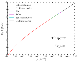
Figure 9: (Color online) Energy per baryon using the TF approximation with the Sk$\chi$450 Skyrme fit model.

The nuclear pasta phases require Coulomb interaction formulas for different dimensions Sharma et al. (2015):

Spherical : (23)

$$V_{p}(r) =4\pi e^{2}\biggl{[}\frac{1}{r}\int_{0}^{r}r^{\prime 2}\rho_{p}(r^{\prime})dr^{\prime}+\int_{r}^{R_{c}}r^{\prime}\rho_{p}(r^{\prime})dr^{\prime}\biggr{]}\,,$$

$$V_{e}(r) =2\pi e^{2}n_{e}\left[R_{c}^{2}-\frac{1}{3}r^{2}\right]\,.$$

Cylindrical : (24)

$$V_{p}(r) =-4\pi e^{2}\biggl{[}\ln(r)\int_{0}^{r}r^{\prime}\rho_{p}(r^{\prime})dr^{\prime}+\int_{r}^{R_{c}}r^{\prime}\ln r^{\prime}\rho_{p}(r^{\prime})dr^{\prime}\biggr{]}\,,$$

$$V_{e}(r) =\pi e^{2}n_{e}R_{c}^{2}\left[1-\frac{r^{2}}{R_{c}^{2}}-2\ln R_{c}\right]\,.$$

Slab : (25)

$$V_{p}(z) =-4\pi e^{2}\left[z\int_{0}^{z}\rho_{p}(z^{\prime})dz^{\prime}+\int_{z}^{R_{c}}z^{\prime}\rho_{p}(z^{\prime})dz^{\prime}\right]\,,$$

$$V_{e}(z) =-2\pi e^{2}n_{e}(z^{2}+R_{c}^{2})\,.$$

Fig. 9 shows the energy per baryon for beta-equilibrated neutron star matter obtained in the TF approximation using the Skyrme parametrization Sk$\chi$450 developed in the present work. As in the case of the LDM model, the ground-state geometry for increasing density proceeds through the sequence {spherical, cylindrical, slab, cylindrical hole, spherical hole, uniform matter} in this order. Each new geometry spans smaller and smaller ranges of densities, and the transition density to the homogeneous phase occurs at $n_{c}=0.084$ fm^-3.

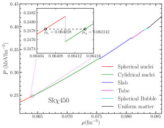
Figure 10: (Color online) Pressure vs. baryon number density using in the TF approximation. A discontinuity in the pressure occurs at the shape transition densities, but the discontinuity region (shown in the inset) is very narrow.

The ground state pressure as a function of density employing the same interaction model is shown in Fig. 10. Unlike the LDM approach, the Thomas-Fermi approximation results in a small discontinuity in the pressure at the interface between each phase when we only compare the energy per baryon to find the ground state of the phase. This is caused by the intrinsic discontinuity in the expressions for the Coulomb energy in the different geometries. The LDM approach enables us to investigate the structure of the pasta phase with fewer parameters, so the pressure discontinuity or proton fraction discontinuity can be small. On the other hand, the more realistic TF method can be done in the space discretization. This means that the discontinuity in the pressure is a natural phenomenon in the case of phase transformation in the TF approximation. When the Maxwell construction is employed, the interval of the density in the coexistence region is so small ($\Delta\rho=0.0001$ fm^-3) that the microscopic structure of the neutron star barely changes. As an example, the two densities of mixed state for spherical shape and cylindrical shape are $\rho_{t_{1}}=0.06406$ and $\rho_{t_{2}}=0.06414$ fm^-3.

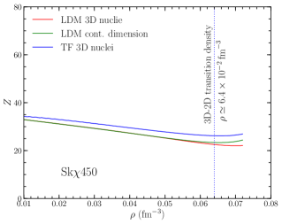
Figure 11: (Color online) Atomic number of heavy nucleus in the Wigner Seitz cell. The dotted line around $\rho=0.064$fm^-3 indicates the transition between 3D nuclei and 2D nuclei.

The choice of LDM vs. TF model also gives rise to differences in nuclear composition. Fig. 11 shows the atomic number of heavy nuclei in the crust of neutron stars. The dotted line indicates the $3D-2D$ phase transition density, which is nearly independent of whether we employ the LDM or the TF model. The atomic number is consistently larger in the TF approximation, differing from the LDM atomic number by roughly two up to the transition to cylindrical geometry. The atomic number in continuous dimension over the $3D-2D$ phase transition density represents the average atomic number in the unit cell. It is not a physical quantity in the crust. Above the $3D-2D$ phase transition density, the TF model gives a larger atomic number since the Wigner-Seitz cell decreases as the total baryon density increases (which means the distance between nuclei decreases) and total number of protons and neutrons increases in the spherical cell.

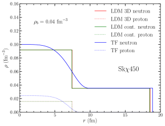
Figure 12: (Color online) Neutron and proton density profiles using three different numerical methods with the Sk$\chi 450$ Skyrme mean field model.

Fig. 12 shows the neutron and proton density profiles in each numerical calculation with the Sk$\chi 450$ interaction. Even if the central densities of protons and neutrons are different in the LDM and TM model, the neutron densities outside the nucleus are nearly the same. This indicates that the density profile is the problem to be solved in order to understand the coexistence of dense and dilute matter. Whatever numerical method is used, the density of the unbound gas of neutrons should be the same under identical physical conditions.

Table 5: Pasta phase transition densities (in units of fm^-3) using the TF method. The numbers in parentheses represent the transition densities with the exchange Coulomb interaction included.

	Sk$\chi 414$	Sk$\chi 450$	Sk$\chi 500$
3DN-2DN	0.0681	0.0641	0.0626
	(0.0682)	(0.0642)	(0.0627)
2DN-1DN	0.0791	0.0755	0.0790
	(0.0795)	(0.0758)	(0.0793)
1DN-2DB	0.0830	0.0809	0.0865
	(0.0838)	(0.816)	(0.0869)
2DB-3DB	0.0852	0.0830	0.0885
	(0.0862)	(0.0836)	(0.0891)
3DB-Uni.	0.0860	0.0835	0.0894
	(0.0869)	(0.0843)	(0.0894)

Table 5 shows the transition density at each phase boundary. The transition density for uniform matter is highly correlated with the saturation density. If the saturation density is greater (as is the case for the Sk$\chi$414 and Sk$\chi$500 Skyrme interactions), uniform nuclear matter is formed at a higher density. The numbers in parentheses indicate the transition density when we include the exchange Coulomb interaction in the numerical calculation. The exchange Coulomb interaction in Eq. (22) gives a negative contribution to the total energy and therefore its presence tends to delay the transitions to higher densities. However, the effects are nearly negligible.

III.4 Thermodynamic instability

In neutron stars, the phase transition from uniform nuclear matter to inhomogeneous nuclear matter takes place when matter begins to exhibit an instability to density fluctuations. Baym et al. Baym et al. (1971) show that the matter is stable when the following relationship is maintained:

$$v_{0}+2(4\pi e^{2}\beta)^{1/2}-\beta k_{TF}^{2}>0\,,$$ (26)

where

$$v_{0}=\frac{\partial\mu_{p}}{\partial\rho_{p}}-\frac{(\partial\mu_{p}/\partial\rho_{n})^{2}}{\partial\mu_{n}/\partial\rho_{n}}\,,$$ (27)

$$\beta=2(Q_{pp}+2Q_{np}\zeta+Q_{nn}\zeta^{2})\,,\quad\zeta=-\frac{\partial\mu_{p}/\partial\rho_{n}}{\partial\mu_{n}/\partial\rho_{n}}\,,$$ (28)

and $k_{TF}$ is the Thomas-Fermi wave number,

$$k_{TF}^{2}=\frac{4e^{2}}{\pi}k_{e}^{2}\,,\quad k_{e}=(3\pi^{2}\rho_{p})^{1/3}\,.$$ (29)

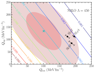
Figure 13: (Color online) Transition density contour plot for the core-crust boundary obtained from thermodynamic instability. The individual points are taken from the modified Skyrme interactions obtained in Ref. Buraczynski and Gezerlis (2016b).

In Skyrme models, $Q_{nn}$ and $Q_{np}$ are given by

$$Q_{nn}=Q_{pp}= \frac{3}{16}\left[t_{1}(1-x_{1})-t_{2}(1+x_{2})\right]\,,$$ (30)

$$Q_{np}=Q_{pn}= \frac{1}{16}\left[3t_{1}(2+x_{1})-t_{2}(2+x_{2})\right]\,.$$

For the three Skyrme parametrizations developed in this work, $Q_{nn}$ and $Q_{np}$ are given by $Q_{nn}=\{107.297,105.458,106.901\}$ MeV-fm^-5 and $Q_{np}=\{119.833,94.759,119.641\}$ MeV-fm^-5 for Sk$\chi 414$, Sk$\chi 450$, and Sk$\chi 500$ respectively. A more conservative uncertainty estimate is obtained by considering a wider set of 31 Skyrme models whose equations of state are similar to that from chiral effective field theory. Fig. 13 shows the resulting confidence contour of $Q_{nn}$ and $Q_{np}$, with the symbol ‘$\mathbf{x}$’ at the center of the ellipse representing the average values. In these calculations the proton and neutron chemical potentials in homogeneous matter are taken from the microscopic equation of state computed from the $\Lambda=450$ MeV chiral nuclear potential. The three individual points labeled “SLy7”, “SLy4”, and “SkM*” come from the modified isovector gradient coupling strengths deduced in recent quantum Monte Carlo studies Buraczynski and Gezerlis (2016b). Fig. 13 indicates that the density for the core-crust boundary is between $\rho=0.082$ fm^-3 and $\rho=0.087$ fm^-3. We infer from the contour plot that the core-crust transition density is proportional to the sum of $Q_{nn}+kQ_{np}$. We propose an empirical formula for the core-crust density with $Q_{nn}$ and $Q_{np}$:

$$\rho_{t}\simeq\rho_{t_{1}}+\alpha Q_{nn}+\beta Q_{np},$$ (31)

which indicates that $Q_{nn}$ and $Q_{np}$ will directly determine the core-crust density.

Table 6: Numerical values for the parameters in Eq. (31).

$\rho_{t_{1}}$ (fm-3)	$9.103\times 10^{-2}\pm 7.065\times 10^{-4}$
$\alpha$ ($\mathrm{MeV}^{-1}\mathrm{fm}^{2}$)	$-3.088\times 10^{-5}\pm 5.257\times 10^{-7}$
$\beta$ ($\mathrm{MeV}^{-1}\mathrm{fm}^{2}$)	$-1.891\times 10^{-5}\pm 1.010\times 10^{-6}$

IV Conclusion

We have studied the composition and structure of neutron star crusts by comparing the energy densities for different pasta phases using both the liquid drop model and the Thomas-Fermi model. The results are based on a new set of extended Skyrme parametrizations derived in the present work that fit the bulk isospin-asymmetric nuclear matter equation of state from $\chi$EFT and the binding energies of doubly-magic nuclei. The neutron star maximum masses obtained from these Skyrme parametrizations are consistent with observations of $2.0M_{\odot}$ neutron stars.

From the LDM and TF calculations, the crust-core transition density is strongly correlated with the saturation density of symmetric nuclear matter. For this reason the extended Skyrme parametrization Sk$\chi$450, which reproduces well both the empirical saturation energy and density, is expected to provide the most reliable prediction for the crust-core interface density. The predicted pressure at the phase boundaries between different pasta geometries is smooth in the LDM but exhibits small discontinuities in the TF approximation. We have studied as well a continuous-dimension LDM that treats the pasta phases as a function of the dense matter volume fraction in the Wigner-Seitz cell. All three methods give a core-crust boundary density around half saturation density, $\rho_{t}=0.084$fm^-3.

Compared to previous works Hebeler et al. (2013); Tews (2017), we analyzed the theoretical uncertainties in the core transition density of neutron stars by varying the gradient terms $Q_{nn}$ and $Q_{np}$. We find that the transition density has a two-dimensional correlation with the $Q$’s. Low values of these gradient term coupling strengths result in an increase in the transition density from the crust to core, which increases the volume of the neutron star crust. The uncertainty in $Q_{nn}$ and $Q_{np}$ can be reduced by microscopic calculations of the static density response function using $\chi$EFT in many-body perturbation theory or quantum Monte Carlo simulations. A more accurate determination of $Q_{nn}$ and $Q_{np}$ will therefore play an important role for improving energy density functionals and to more accurately predict the density at a neutron star’s core-crust boundary.

We find that nuclear pasta exists within the density range between $\rho=0.065$ fm^-3 and $0.090$ fm^-3. Macroscopically it exists within a 100 m thickness in the inner crust of a neutron star with 1.4$M_{\odot}$. The spherical hole phase exists within the density range of $\Delta\rho=0.002$ fm^-3 at most. This means that spherical holes exist only within a $\Delta R=5$ m range in neutron stars, which might be destroyed in fast rotating neutron stars because of tidal deformation. Our results are similar to the previous works of Oyamatsu Oyamatsu (1993) and Sharma et al. Sharma et al. (2015), who employed phenomenological models with equations of state similar to the predictions from $\chi$EFT.

References

- Weber (2005) F. Weber, Prog. Part. Nucl. Phys. 54, 193 (2005).
- Alford et al. (2005) M. Alford, M. Braby, M. Paris, and S. Reddy, Astrophys. J. 629, 969 (2005).
- Weissenborn et al. (2011) S. Weissenborn, I. Sagert, G. Pagliara, M. Hempel, and J. Schaffner-Bielich, Astrophys. J. 740, L14 (2011).
- Schaffner-Bielich et al. (2002) J. Schaffner-Bielich, M. Hanauske, H. Stoecker, and W. Greiner, Phys. Rev. Lett. 89, 171101 (2002).
- Weissenborn et al. (2012a) S. Weissenborn, D. Chatterjee, and J. Schaffner-Bielich, Nucl. Phys. A881, 62 (2012a).
- Weissenborn et al. (2012b) S. Weissenborn, D. Chatterjee, and J. Schaffner-Bielich, Phys. Rev. C 85, 065802 (2012b), [Erratum: Phys. Rev. C 90, 019904 (2014)].
- Lim et al. (2015) Y. Lim, C. H. Hyun, K. Kwak, and C.-H. Lee, Int. J. Mod. Phys. E 24, 1550100 (2015).
- Chatterjee and Vidaña (2016) D. Chatterjee and I. Vidaña, Eur. Phys. J. A 52, 29 (2016).
- Baym (1973) G. Baym, Phys. Rev. Lett. 30, 1340 (1973).
- Thorsson et al. (1994) V. Thorsson, M. Prakash, and J. M. Lattimer, Nucl. Phys. A572, 693 (1994).
- Glendenning and Schaffner-Bielich (1998) N. K. Glendenning and J. Schaffner-Bielich, Phys. Rev. Lett. 81, 4564 (1998).
- Lim et al. (2014) Y. Lim, K. Kwak, C. H. Hyun, and C.-H. Lee, Phys. Rev. C 89, 055804 (2014).
- Weinberg (1979) S. Weinberg, Physica A 96, 327 (1979).
- Epelbaum et al. (2009a) E. Epelbaum, H.-W. Hammer, and U.-G. Meißner, Rev. Mod. Phys. 81, 1773 (2009a).
- Machleidt and Entem (2011) R. Machleidt and D. R. Entem, Phys. Rept. 503, 1 (2011).
- Epelbaum et al. (2015) E. Epelbaum, H. Krebs, and U.-G. Meißner, Eur. Phys. J. A 51, 53 (2015).
- Entem et al. (2015) D. R. Entem, N. Kaiser, R. Machleidt, and Y. Nosyk, Phys. Rev. C 91, 014002 (2015).
- Epelbaum et al. (2009b) E. Epelbaum, H. Krebs, D. Lee, and U. G. Meißner, Eur. Phys. J. A 40, 199 (2009b).
- Hebeler and Schwenk (2010) K. Hebeler and A. Schwenk, Phys. Rev. C 82, 014314 (2010).
- Hebeler et al. (2011) K. Hebeler, S. K. Bogner, R. J. Furnstahl, A. Nogga, and A. Schwenk, Phys. Rev. C 83, 031301 (2011).
- Coraggio et al. (2013) L. Coraggio, J. W. Holt, N. Itaco, R. Machleidt, and F. Sammarruca, Phys. Rev. C 87, 014322 (2013).
- Gezerlis et al. (2013) A. Gezerlis, I. Tews, E. Epelbaum, S. Gandolfi, K. Hebeler, A. Nogga, and A. Schwenk, Phys. Rev. Lett. 111, 032501 (2013).
- Tews et al. (2013) I. Tews, T. Krüger, K. Hebeler, and A. Schwenk, Phys. Rev. Lett. 110, 032504 (2013).
- Coraggio et al. (2014) L. Coraggio, J. W. Holt, N. Itaco, R. Machleidt, L. E. Marcucci, and F. Sammarruca, Phys. Rev. C 89, 044321 (2014).
- Roggero et al. (2014) A. Roggero, A. Mukherjee, and F. Pederiva, Phys. Rev. Lett. 112, 221103 (2014).
- Wlazłowski et al. (2014) G. Wlazłowski, J. W. Holt, S. Moroz, A. Bulgac, and K. J. Roche, Phys. Rev. Lett. 113, 182503 (2014).
- Carbone et al. (2014) A. Carbone, A. Rios, and A. Polls, Phys. Rev. C 90, 054322 (2014).
- Tews et al. (2016) I. Tews, S. Gandolfi, A. Gezerlis, and A. Schwenk, Phys. Rev. C 93, 024305 (2016).
- Drischler et al. (2014) C. Drischler, V. Somà, and A. Schwenk, Phys. Rev. C 89, 025806 (2014).
- Wellenhofer et al. (2016) C. Wellenhofer, J. W. Holt, and N. Kaiser, Phys. Rev. C 93, 055802 (2016).
- Tolos et al. (2008) L. Tolos, B. Friman, and A. Schwenk, Nucl. Phys. A A806, 105 (2008).
- Wellenhofer et al. (2014) C. Wellenhofer, J. W. Holt, N. Kaiser, and W. Weise, Phys. Rev. C 89, 064009 (2014).
- Wellenhofer et al. (2015) C. Wellenhofer, J. W. Holt, and N. Kaiser, Phys. Rev. C 92, 015801 (2015).
- Bogner et al. (2009) S. K. Bogner, R. J. Furnstahl, and L. Platter, Eur. Phys. J. A 39, 219 (2009).
- Holt et al. (2011) J. W. Holt, N. Kaiser, and W. Weise, Eur. Phys. J. A 47, 128 (2011).
- Kaiser (2012) N. Kaiser, Eur. Phys. J. A 48, 36 (2012).
- Gandolfi et al. (2011) S. Gandolfi, J. Carlson, and S. C. Pieper, Phys. Rev. Lett. 106, 012501 (2011).
- Buraczynski and Gezerlis (2016a) M. Buraczynski and A. Gezerlis, Phys. Rev. Lett. 116, 152501 (2016a).
- Lykasov et al. (2008) G. I. Lykasov, C. J. Pethick, and A. Schwenk, Phys. Rev. C 78, 045803 (2008).
- Davesne et al. (2015) D. Davesne, J. W. Holt, A. Pastore, and J. Navarro, Phys. Rev. C 91, 014323 (2015).
- Holt et al. (2012) J. W. Holt, N. Kaiser, and W. Weise, Nucl. Phys. A 876, 61 (2012).
- Holt et al. (2013a) J. W. Holt, N. Kaiser, and W. Weise, Phys. Rev. C 87, 014338 (2013a).
- Ravenhall et al. (1983a) D. G. Ravenhall, C. J. Pethick, and J. R. Wilson, Phys. Rev. Lett. 50, 2066 (1983a).
- Douchin and Haensel (2001) F. Douchin and P. Haensel, Astron. Astrophys. 380, 151 (2001).
- Newton et al. (2013) W. G. Newton, M. Gearheart, and B.-A. Li, The Astrophysical Journal Supplement Series 204, 9 (2013).
- Oyamatsu (1993) K. Oyamatsu, Nucl. Phys. A561, 431 (1993).
- Okamoto et al. (2013) M. Okamoto, T. Maruyama, K. Yabana, and T. Tatsumi, Phys. Rev. C 88, 025801 (2013).
- Newton and Stone (2009) W. G. Newton and J. R. Stone, Phys. Rev. C 79, 055801 (2009).
- Pais and Stone (2012) H. Pais and J. R. Stone, Phys. Rev. Lett. 109, 151101 (2012).
- Schuetrumpf and Nazarewicz (2015) B. Schuetrumpf and W. Nazarewicz, Phys. Rev. C 92, 045806 (2015).
- Horowitz et al. (2005) C. J. Horowitz, M. A. Pérez-García, D. K. Berry, and J. Piekarewicz, Phys. Rev. C 72, 035801 (2005).
- Sonoda et al. (2008) H. Sonoda, G. Watanabe, K. Sato, K. Yasuoka, and T. Ebisuzaki, Phys. Rev. C 77, 035806 (2008).
- Schneider et al. (2013) A. S. Schneider, C. J. Horowitz, J. Hughto, and D. K. Berry, Phys. Rev. C 88, 065807 (2013).
- Brown and Schwenk (2014) B. A. Brown and A. Schwenk, Phys. Rev. C 89, 011307 (2014).
- Bulgac et al. (2015) A. Bulgac, M. M. Forbes, and S. Jin, arXiv:1506.09195 (2015).
- Rrapaj et al. (2016) E. Rrapaj, A. Roggero, and J. W. Holt, Phys. Rev. C 93, 065801 (2016).
- Entem and Machleidt (2003) D. R. Entem and R. Machleidt, Phys. Rev. C 68, 041001 (2003).
- Holt and Kaiser (2016) J. W. Holt and N. Kaiser, arXiv:1612.04309 (2016).
- Holt et al. (2013b) J. W. Holt, N. Kaiser, and W. Weise, Prog. Part. Nucl. Phys. 73, 35 (2013b).
- Holt et al. (2016) J. W. Holt, M. Rho, and W. Weise, Phys. Rept. 621, 2 (2016).
- Elliott et al. (2013) J. B. Elliott, P. T. Lake, L. G. Moretto, and L. Phair, Phys. Rev. C 87, 054622 (2013).
- Audi et al. (2015) G. Audi et al., Atom. Data Nucl. Data Tabl. 103, 1 (2015).
- Dutra et al. (2012) M. Dutra, O. Lourenço, J. S. Sá Martins, A. Delfino, J. R. Stone, and P. D. Stevenson, Phys. Rev. C 85, 035201 (2012).
- De Vries et al. (1987) H. De Vries, C. W. De Jager, and C. De Vries, Atom. Data Nucl. Data Tabl. 36, 495 (1987).
- Steiner et al. (2010) A. W. Steiner, J. M. Lattimer, and E. F. Brown, Astrophys. J. 722, 33 (2010).
- Demorest et al. (2010) P. Demorest, T. Pennucci, S. Ransom, M. Roberts, and J. Hessels, Nature 467, 1081 (2010).
- Antoniadis et al. (2013) J. Antoniadis et al., Science 340, 6131 (2013).
- Baym et al. (1971) G. Baym, H. A. Bethe, and C. Pethick, Nucl. Phys. A175, 225 (1971).
- Ruester et al. (2006) S. B. Ruester, M. Hempel, and J. Schaffner-Bielich, Phys. Rev. C73, 035804 (2006).
- Stoitsov et al. (2003) M. V. Stoitsov, J. Dobaczewski, W. Nazarewicz, S. Pittel, and D. J. Dean, Phys. Rev. C68, 054312 (2003).
- Goriely et al. (2013) S. Goriely, N. Chamel, and J. M. Pearson, Phys. Rev. C88, 024308 (2013).
- Moller et al. (2016) P. Moller, A. J. Sierk, T. Ichikawa, and H. Sagawa, Atom. Data Nucl. Data Tabl. 109, 1 (2016).
- Duflo and Zuker (1995) J. Duflo and A. P. Zuker, Phys. Rev. C52, R23 (1995).
- Hilaire and Girod (2007) S. Hilaire and M. Girod, The European Physical Journal A 33, 237 (2007).
- Ravenhall et al. (1983b) D. G. Ravenhall, C. J. Pethick, and J. M. Lattimer, Nucl. Phys. A407, 571 (1983b).
- Lattimer and Swesty (1991) J. M. Lattimer and F. D. Swesty, Nucl. Phys. A535, 331 (1991).
- Sharma et al. (2015) B. K. Sharma, M. Centelles, X. Viñas, M. Baldo, and G. F. Burgio, Astron. Astrophys. 584, A103 (2015).
- Buraczynski and Gezerlis (2016b) M. Buraczynski and A. Gezerlis, arXiv:1608.03598 (2016b).
- Hebeler et al. (2013) K. Hebeler, J. M. Lattimer, C. J. Pethick, and A. Schwenk, Astrophy. J. 773, 11 (2013).
- Tews (2017) I. Tews, Phys. Rev. C 95, 015803 (2017).