Molecular simulations of entangled defect structures around nanoparticles in nematic liquid crystals

Abstract

We investigate the defect structures forming around two nanoparticles in a Gay-Berne nematic liquid crystal using molecular simulations. For small separations, disclinations entangle both particles forming the figure of eight, the figure of omega and the figure of theta. These defect structures are similar in shape and occur with a comparable frequency to micron-sized particles studied in experiments. The simulations reveal fast transitions from one defect structure to another suggesting that particles of nanometre size cannot be bound together effectively. We identify the ‘three-ring’ structure observed in previous molecular simulations as a superposition of the different entangled and non-entangled states over time and conclude that it is not itself a stable defect structure.

I Introduction

Spherical particle inclusions in liquid crystals distort the orientational order of the surrounding molecules inducing topological defects. Defect regions are defined by the absence of orientational order, i.e. the liquid crystal is melted. Such defects arise due to the competition between liquid crystal molecules trying to align along the average molecular direction, called the director, and trying to fulfil the surface anchoring condition of the nanoparticle. For small particles or particles confined to a thin nematic cell, the defect region forms a defect ring near the equator of the particle with respect to the director, commonly referred to as a Saturn ring Stark (2002). Particles surrounded by a Saturn ring show quadrupolar interactions due to the symmetry of the director field surrounding them; hence such particles are called quadrupoles. For two quadrupoles in close vicinity, entangled defects were found to spontaneously arise when the surrounding nematic is distorted. Using laser tweezers, which allow easy manipulation with great precision, a range of reproducible entangled objects have been found Guzmán et al. (2003); Araki and Tanaka (2006); Ravnik et al. (2007); Škarabot et al. (2008); Ravnik and Žumer (2009a); Čopar and Žumer (2011); Kim et al. (2004). Here ‘entangled’ means that both particles are surrounded by a single defect line, commonly referred to as a disclination line. The three main structures comprise the figure of eight ($\infty$), the figure of omega ($\Omega$) and the figure of theta ($\Theta$). Schematics are shown in Fig. 1. Micrographs of these entangled defect structures observed in experiments can be found in Fig. 4 of Tkalec and Muševič (2013).

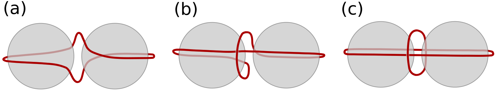
Figure 1: Schematic of two nanoparticles (grey) in nematic host (not shown) entangled by a disclination line (dark red) forming the (a) figure of eight $\infty$, (b) the figure of omega $\Omega$ and (c) the figure of theta $\Theta$.

For the figure of eight defect a single disclination line winds around the particles in the manner shown in Fig. 1(a). The figure of omega consists of one disclination line that surrounds both particles near the equator, entering into the space between the particles to descibe a shape similar to the Greek letter $\Omega$. The figure of theta consists of a disclination line surrounding both particles and an additional defect loop in the plane in between the particles. Note the spontaneous symmetry breaking for the first two of these structures due to their chirality. The two states are degenerate and hence left-handed and right-handed structures occur with the same frequency.

These entangled defects were observed in experiments and predicted numerically for micron-sized particles using phenomenological mean-field calculations based on Landau-de Gennes free energy minimisation Ravnik and Žumer (2009b, a). At first glance these entangled structures appear to disobey the restriction that the net topological charge within the liquid crystal must be zero; however Čopar and Žumer (2011) resolved this apparent contradiction with the introduction of a self-linking number.

A closer look at the different defect structures reveals that entangled defects differ only within a tetrahedral region. Theoretically, by rotating the tetrahedron, one entangled state can be transformed into another Čopar and Žumer (2011). In practice, this is equivalent to cutting and reconnecting the disclination lines, whereas in experiments this rewiring is achieved by locally applying laser tweezers to heat the region around the tetrahedron.

Molecular simulations of two quadrupoles in close vicinity have shown a three-ring structure for particle inclusions of nanometre size Grollau et al. (2003); Kim et al. (2004); Guzmán et al. (2003). This structure is similar to the figure of $\Theta$; however the inner loop connects with the outer loop at two nodes. Two possible explanations have been proposed as to why the structure differs from the ones observed in experiments. Earlier studies declared it a transient state Araki and Tanaka (2006). It was later proposed Hung (2009) that instead the size of the particles is crucial and that the three-ring structure appears for particles of nanometre scale, whereas micron-sized particles form only the three different entangled defects ($\infty$, $\Theta$ and $\Omega$). In this paper we propose an alternative explanation for the three-ring structure.

The system of two entangled particles can be thought of as a building block for more complex systems. Recent work has shown one-dimensional Ravnik et al. (2007) as well as two-dimensional Ravnik and Žumer (2009c); Araki et al. (2013); Tkalec et al. (2011) aggregates, where the disclination line winds around all the particles. Entanglement has also been observed for microspheres and microfibres Nikkhou et al. (2015). When bringing many particles into close vicinity, knotted structures can be created Jampani et al. (2011); Tkalec et al. (2011); Čopar et al. (2015). By applying the laser tweezers in unknotted regions, additional knots can be created and vice versa. Wood et al. (2011) showed that liquid crystals with a high number of nanoparticle inclusions can be used to synthesise a soft solid, which shows high rigidity due to a network of entangled defect lines. These materials have important features for potential use in biosensors Agarwal et al. (2008).

Entangled and knotted systems can be manipulated not only by the use of laser tweezers, but also by using strong local electric fields, hydrodynamic flow, temperature changes and the use of different boundary conditions and confined geometries. This allows the creation and modification of defects in liquid crystals in a rather controllable way and hence a variety of complex systems can be designed.

In this paper we outline a model to efficiently simulate entangled nanoparticles. Simulation details are given in Section II. In Section III we present how the different defect types are automatically categorised. The results, in particular the time scales and dynamics of transitions from one entangled defect structure to another, are discussed in Section IV. In addition, the origin of the three-ring structure, the only structure observed in previous molecular simulations, is identified. Conclusions are drawn in Section V

II Model and simulation details

The entanglement was studied by simulating several systems with nanoparticle inclusions of various sizes and separations. The nematic host was simulated using the well-known soft Gay-Berne potential (see appendix A), a coarse-grained single-site potential that represents the interaction energies between two elongated particles. We chose a length-to-width ratio of $\kappa=3$. The remaining Gay-Berne coefficients were set to $\mu=1$, $\nu=3$ and $\kappa^{\prime}=5$ and a potential cutoff of $5\sigma_{0}$ was applied. Note that reduced units were used throughout by setting $\sigma_{0}=\epsilon_{0}=1$ and the molecular mass $m_{0}=1$ leading to a basic unit of time $\tau_{0}=\sigma_{0}\sqrt{m_{0}/\epsilon_{0}}$. The moment of inertia was set to $I=0.5m_{0}\sigma_{0}^{2}$ assuming uniform mass distribution. The initial director orientation was chosen to lie along the $z$ direction.

Spherical particle inclusions of radius $R_{\text{NP}}$ were placed in the box, interacting with the liquid crystal molecules via a purely repulsive Lennard-Jones potential (see appendix B). Their positions were fixed throughout the simulation. The system was simulated for particles separated along $x$ with a surface-to-surface separation of $\Delta$. Five different systems of nematics with nanoparticle inclusions of radii $R_{\text{NP}}=10\sigma_{0}$, $15\sigma_{0}$ and $20\sigma_{0}$ were studied. In all cases, box dimensions were chosen to give a bulk density $\rho\sim 0.3$, and the temperature was chosen to be $T=3.0$, which, for this system, gives a nematic liquid crystal phase. Simulation details are given in the following subsections.

Nanoparticles of radius $R_{\text{NP}}=10\sigma_{0}$

Two spherical particle inclusions of radius $R_{\text{NP}}=10\sigma_{0}$ were placed in the box, separated along $x$, with $\Delta=2.94\sigma_{0}$ as well as $\Delta=10.3\sigma_{0}$. A cubic simulation box of length $\sim 120\sigma_{0}$ with periodic boundaries was used. The large simulation box is necessary to avoid any interference between nanoparticles through the boundaries. The system was equilibrated over $1.6\text{\times}{10}^{6}$ time steps using an $NpT$ ensemble, followed by a production run, also in the $NpT$ ensemble, of $2.5\text{\times}{10}^{5}$ time steps with a time step $\Delta t=0.004$. Molecular positions and orientations were stored every $500$ time steps. The total number of Gay-Berne molecules was $512\,000$.

Nanoparticles of radius $R_{\text{NP}}=15\sigma_{0}$

The simulation was repeated with particles of size $R_{\text{NP}}=15\sigma_{0}$ separated along $x$ with $\Delta=5\sigma_{0}$ as well as $\Delta=10\sigma_{0}$. Most other simulation details were unchanged. Two modifications were made to reduce computational cost.

The first modification consists of the introduction of flat walls at the $z$ boundaries. A simple Lennard-Jones 12-6 function of the $z$ coordinate, relative to the wall, was utilised with ${\epsilon_{0}}={\sigma_{0}}={1}$ and a potential cutoff of $2.5\sigma_{0}$. This has the advantage that $L_{z}$ can be chosen to be smaller than in the system described above, without the danger of long-range interactions between images of nanoparticles across the boundaries; this type of boundary also stabilizes the bulk director in the $z$ direction. $L_{z}$ must be sufficiently large to accommodate the density and order parameter fluctuations near the walls, ensuring bulk behaviour in the centre of the simulation box. A system snapshot of Gay-Berne molecules near a Lennard-Jones wall can be seen in Fig.  2 (a). One can clearly see layering near the wall that disappears quickly further away from the wall.

The second modification consists of the reduction of the simulation box length $L_{x}$ to $2R_{\text{NP}}+\Delta$ (so $L_{x}=35\sigma_{0}$ for $\Delta=5\sigma_{0}$ and $L_{x}=40\sigma_{0}$ for $\Delta=10\sigma_{0}$) and the placement of one nanoparticle at ($\pm\frac{1}{2}L_{x}$,0,0), illustrated in Fig. 2(b). With periodic boundary conditions along $x$ this represents an infinite chain of nanoparticles along the $x$ direction ($L_{y}$ remains large enough to avoid periodic self-interaction). This allows the reduction of the total number of Gay-Berne molecules by over 50$\%$; choosing $L_{y}=L_{z}\sim 136\sigma_{0}$ in both cases, with $N=$182\,000$$ for $\Delta=5\sigma_{0}$ and $N=$210\,000$$ for $\Delta=10\sigma_{0}$, gave a bulk density $\rho\sim 0.3$. The system was equilibrated over $7.5\text{\times}{10}^{5}$ time steps ($\Delta t=0.004$) using an $NVT$ ensemble, followed by a production run ($NVT$ ensemble) of $4\text{\times}{10}^{5}$ time steps. Molecular positions and orientations were stored every $500$ time steps.

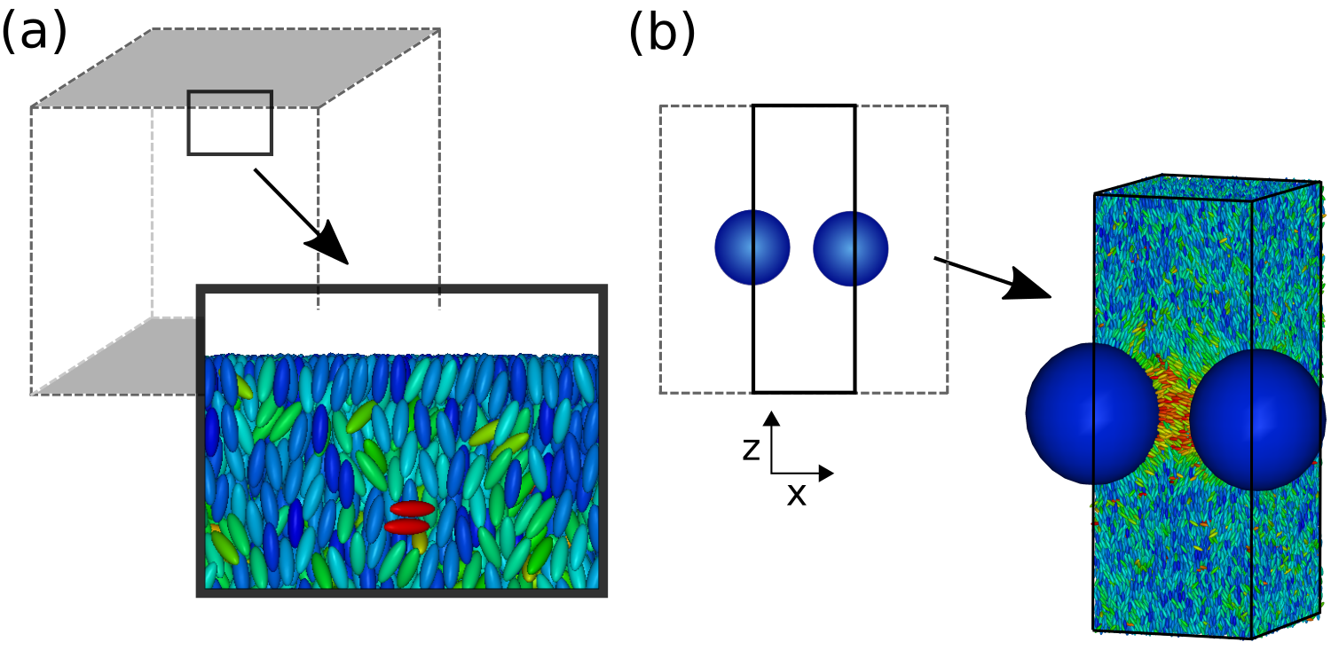
Figure 2: Schematic of simulation box. (a) Typical snapshot of Gay-Berne molecules near a Lennard-Jones wall applied near the $z$ boundaries indicated in grey. Gay-Berne molecules were colour-coded according to their orientation with respect to the director. (b) Two-dimensional view of the simulation box (grey dashed region) in the $x$-$z$ plane. The black box indicates the area used to simulate an infinitely long one-dimensional chain of nanoparticles (blue). The box length along $y$ was unchanged. Molecular snapshot shows a slice of the new simulation box with the nanoparticles at its centre.

Nanoparticles of radius $R_{\text{NP}}=20\sigma_{0}$

In this simulation the nanoparticle radius was increased to $R_{\text{NP}}=20\sigma_{0}$. Other system parameters were chosen as for the system with $R_{\text{NP}}=15\sigma_{0}$. No wall potential was applied and instead periodic boundaries were used across $z$. The total number of Gay-Berne molecules was $N=$214\,000$$ with a moment of inertia of $I=2.5m_{0}\sigma_{0}^{2}$. The box dimensions were chosen to be $L_{x}=50\sigma_{0}$ and $L_{y}=L_{z}\sim 120\sigma_{0}$; hence the separation between neighbouring nanoparticles was $\Delta=10\sigma_{0}$. The system was equilibrated over $8\text{\times}{10}^{5}$ time steps ($\Delta t=0.004$) using an $NVT$ ensemble, followed by a production run ($NVE$ ensemble) of $6.5\text{\times}{10}^{5}$ time steps. Molecular positions and orientations were stored every $500$ time steps.

III Automated characterisation of defect types

To identify defect regions for the system snapshots stored, a weighted order tensor was calculated following the approach suggested by Callan-Jones et al. (2006). This quasi-continuous tensor is given by

$$D_{mm^{\prime}}(\bm{r})=\frac{1}{N(V_{s})}\sum_{i\in V_{s}}w(|\bm{r}_{i}-\bm{r}|)u_{m}^{i}u_{m^{\prime}}^{i}\>,$$ (1)

where $N(V_{s})$ is the number of molecules in the spherical sampling volume $V_{s}$ with radius $r_{k}$ centred at $\bm{r}$, $\bm{r}_{i}$ is the position vector of particle $i$ and $u^{i}$ is the component of its orientation vector with $m,m^{\prime}=x,y,z$. $w(|\bm{r_{i}}-\bm{r}|)$ is a weighting function with the constraint

$$\sum_{i\in V_{s}}w(|\bm{r_{i}}-\bm{r}|)=1\>.$$ (2)

We choose a cubic b-spline, which is a piecewise continuous cubic polynomial approximation to a Gaussian function Bartels et al. (1987), scaled to obey Equation (2):

$$w(r_{w})=\left\{\begin{array}[]{l l}\frac{1}{6}(3|r_{w}|^{3}-6r_{w}^{2}+4)&\quad 0\leq|r_{w}|\leq 1\\ \frac{1}{6}(2-|r_{w}|)^{3}&\quad 1\leq|r_{w}|\leq 2\\ 0&\quad\text{else,}\end{array}\right.$$ (3)

where $r_{w}=2|\bm{r_{i}}-\bm{r}|/r_{k}$. $w$ is zero if $|\bm{r}_{i}-\bm{r}|$ is greater than the radius $r_{k}$. $r_{k}$ was chosen to be 7.3$\sigma_{0}$, which corresponds to having roughly 30 Gay-Berne molecules inside the sampling volume $V_{s}$. The eigenvalues of $D$ are labelled $\lambda_{1}\geq\lambda_{2}\geq\lambda_{3}$. The uniaxial order of a grid point is defined as its alignment to the local nematic director field, and is given by the Westin metric $c_{l}=\lambda_{1}-\lambda_{2}$, which is zero in the isotropic region and unity in perfectly ordered regions. Within the bulk $c_{l}$ undergoes small variations, whereas significant reductions indicate defect regions. We identified $c_{l}<0.05$ as an appropriate threshold to determine defect core regions.

For each system snapshot the weighted order tensor $D$ was calculated on a regular 3D grid with a spacing of $0.25\sigma_{0}$ and defect regions were evaluated, which allowed the subsequent determination of the defect structure. Due to the high number of snapshots this process was automated and the defects classified as follows.

All grid points of the defect core, corresponding to $c_{l}<0.05$, were identified and stored; all points with values above the threshold were discarded We did not further distinguish between different values of $c_{l}$.

To separate points into disclination lines, the flood-fill algorithm was used. To begin, an arbitrary starting point is chosen and added to a queue. The algorithm then consists of removing the first point from the queue, adding all its neighbours to the queue, then adding the removed point to a list $L_{i}$. This step is repeated until the queue is empty, at which point the list $L_{i}$ corresponds to a discrete contiguous volume of points. A new starting point is then chosen to form the seed of a new list $L_{j}$, and the process continues until all points have been assigned to a disclination line.

Note that since only defect regions were stored, a point may not have neighbours in all six directions. To efficiently implement the flood-fill algorithm for such an irregular array, a linked-list connectivity graph was constructed such that each point stores references to its neighbours. Since disclination lines can only exist in the form of closed loops (or lines across periodic boundaries), each defect line was checked for this criterion. For coarser grids, noise artefacts in the data sometimes caused hairline breaks in the disclination lines, causing them to have ‘endpoints’. These endpoints could be identified by examining the neighbour-to-neighbour distance between points, estimated using the all-pairs shortest-path Floyd-Warshall algorithm Cormen et al. (2001) to find the two points separated by the longest path. Two endpoints in close proximity, and with no other endpoint nearby, could be automatically joined and their lists merged.

While the Floyd-Warshall algorithm gives a deterministic measure of distance along the disclination line, it scales with the cube of the number of points $P$ and would be too slow for larger systems. The sparsity of the point-connectivity graph would make a per-point Dijkstra approach more promising in these cases, with $\mathcal{O}(P^{2}\log P)$ scaling Cormen et al. (2001). Coarse-graining could also be used to reduce the effective $P$.

The length of a disclination line is of particular interest because it is proportional to its associated energy. Most of our disclination lines were well-behaved, allowing the use of a ballistic ‘sphere-tracking’ approach which is much faster than connectivity-based approaches. An arbitrary starting point is chosen, and a second is chosen nearby. We define the unit vector connecting these two points as our (arbitrary) initial direction of travel, and move a short distance along it. The average position of the defect line near the destination was calculated by averaging the positions of the 10 nearest points, which was enough to encapsulate the cross-section of the line for our grid size. The new direction of travel is set to be the vector connecting the previous position and this new average, and this direction is followed from the most recent average to arrive at the new destination. The process continues until the initial starting point is reached. The length was estimated by summing the distances between neighbouring averaged positions. This method proved to be accurate and reliable. In Fig. 3 the red points indicated the average positions calculated using this method for an example snapshot.

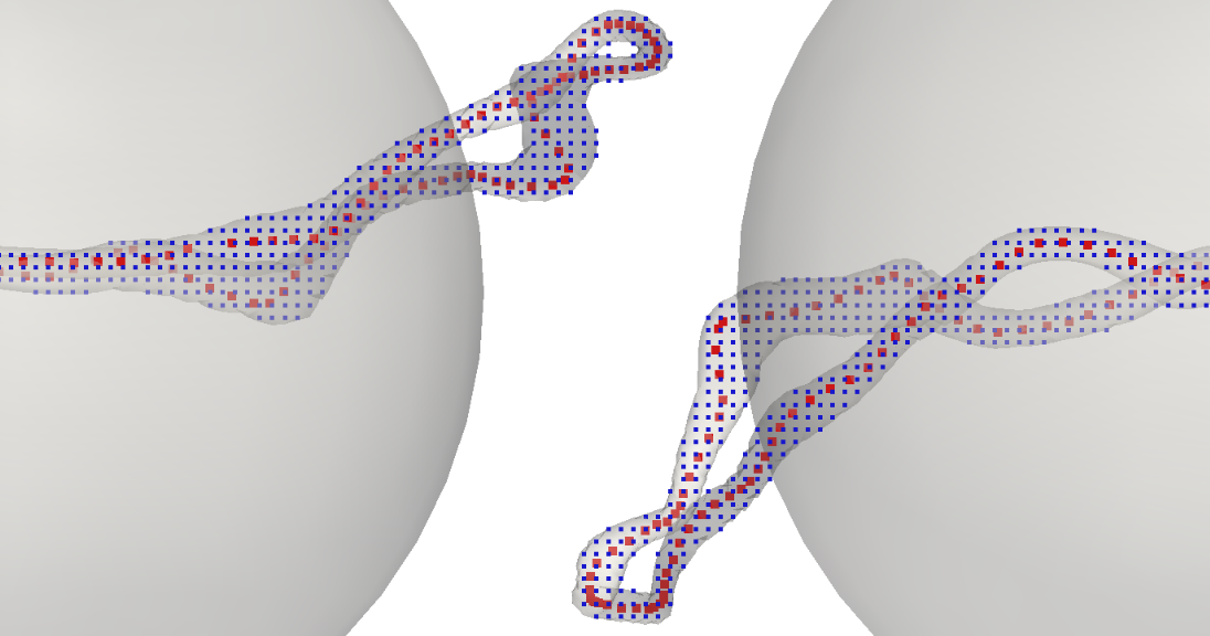
Figure 3: Disclination lines around two nanoparticles (grey). Blue small dots correspond to data points with $c_{l}$ below the threshold and red large points correspond to points calculated using the ‘sphere-tracking’ (see description in text).

To accurately distinguish between the different defect types the connections between the red regions in Fig. 4 were evaluated using the flood-fill algorithm. Here the boundaries were treated as fixed. The connections in conjunction with the number of disclinations and their respective lengths allow us to determine the defect structure. For the figure of eight we further distinguished the direction of the twist, depending on which path crosses over the other. In over $99.9\%$ of the snapshots this automated analysis was conclusive; inconclusive exceptions were inspected visually.

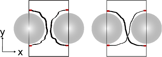
Figure 4: Schematic of two nanoparticles (grey) and the surrounding disclination lines (black) in the $x$-$y$ plane. Red regions show the starting areas for the flood-fill to distinguish different defect structures. Depending on which red regions are connected the defect type was determined.

IV Results and discussion

In Fig. 5 the different defect structures over time are shown for all five systems.

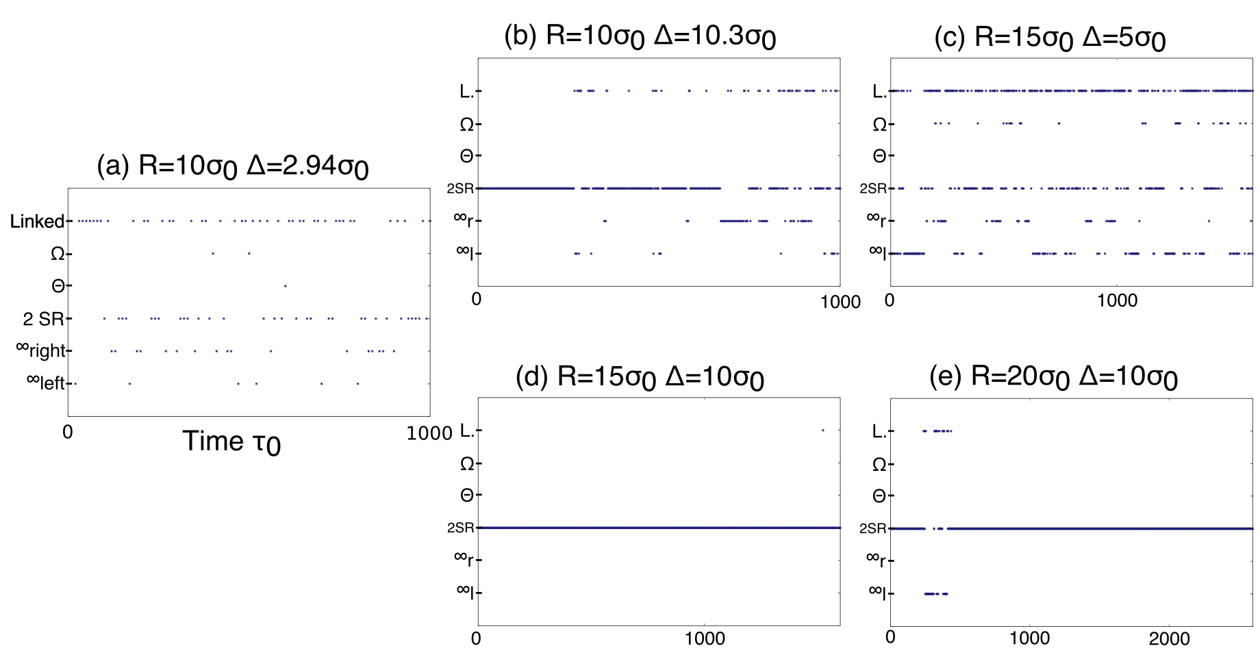
Figure 5: Different defect structures shown over time for all five simulations. Particle radius and surface-to-surface separation are given by $R$ and $\Delta$ respectively. The defect types are labelled as following: intermediate defect structure (Linked), figure of omega ($\Omega$), figure of theta ($\Theta$), two separate Saturn rings (2 SR) and figure of eight ($\infty$). Subscripts indicate right- and left-handed twist.

In total five different structures were observed: separated Saturn rings, figure of eight, figure of omega, figure of theta as well as an intermediate structure, where the two distant parts of the disclination are linked. With the exception of the intermediate defect structure all these defect structures were also observed in experiments and using Landau-de Gennes minimisation for micron-sized particles Ravnik et al. (2009). For each of these structures a typical example is shown in Fig. 6.

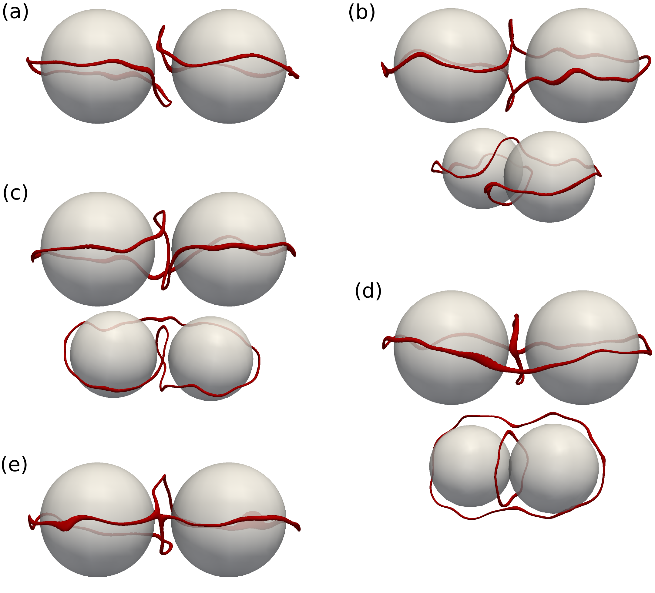
Figure 6: Defect structures (red) observed for two nanoparticles (grey) of radius $R_{\text{NP}}=10\sigma_{0}$ in close proximity ($\Delta=2.94\sigma_{0}$). Some are shown from two angles for clarity. (a) two separate Saturn rings (2 SR), (b) figure of eight ($\infty$), (c) figure of omega ($\Omega$), (d) figure of theta ($\Theta$) and (e) intermediate defect structure (Linked).

The only non-entangled structure found was two nanoparticles surrounded by a Saturn ring each shown in Fig. 6(a). The Saturn rings are strongly bent away from each other to minimise the distortion of the director field, which minimises free energy. The bending effect was also observed for Landau-de Gennes free energy minimisations Ravnik et al. (2009). Fig. 6(b–d) show typical snapshots of the figure of eight, the figure of omega and the figure of theta from two different angles. The shape of the defect line is in good agreement with the observations for micron-sized particles in experiments. Fig. 6(e) shows an intermediate structure, where two distant segments of the disclination line are linked. For all five structures thermal fluctuations of the disclinations are visible, since time averaging was avoided.

For nanoparticles with radius $R_{\text{NP}}=10\sigma_{0}$ the defect structure transitions frequently between different structures and no structure persists for longer than $\sim 250\tau_{0}$. When comparing the results for the two different separations, one can see that transitions are more frequent for the smaller separation, suggesting a smaller barrier to interconversion. It appears, at least for the time simulated, that two separate Saturn rings are the most frequent structure. The figure of eight can be seen occasionally, whereas the figure of theta and omega are very rare. The exact frequencies are given in Table 1 for all five simulations. The intermediate linked structure was observed frequently. This is interesting as this structure is not observed in experiments, suggesting that it is unstable, which in turn suggests that the particle size does indeed have a significant impact on the energy barriers of the entanglement.

For particles with radius $R_{\text{NP}}=15\sigma_{0}$ and a surface-to-surface separation of $\Delta=5\sigma_{0}$, entangled defect structures formed, and the frequency of transitions is very similar to that for the smaller particles. With the separation increased to $\Delta=10\sigma_{0}$ no transitions were observed throughout the production run and the only structure seen was the two separate Saturn rings. For particles with radius $R_{\text{NP}}=20\sigma_{0}$ and a surface-to-surface separation of $\Delta=10\sigma_{0}$, two Saturn rings were observed most frequently. For a short period, $\sim 150\tau_{0}$, the figure of eight with a right-hand twist formed.

Table 1: Frequency of observations of different entangled defect structures for a different particle radii and separations given in $\%$. $R_{\text{NP}}$ and $\Delta$ are the particle radii and their surface-to-surface separation respectively. Notation for different defect structures as introduced in Fig.  6.

	Defect structure frequency (in $\%$)
$\Delta(\sigma_{0})$	2 SR	$\infty_{\text{left}}$	$\infty_{\text{right}}$	$\Theta$	$\Omega$	Linked
$R_{\text{NP}}=10\sigma_{0}$
$2.94$	$31.7$	$5.9$	$16.8$	$1.0$	$2.0$	$42.6$
$10.30$	$71.9$	$3.6$	$13.4$	$0.0$	$0.0$	$11.2$
$R_{\text{NP}}=15\sigma_{0}$
$5.0$	$24.3$	$22.2$	$9.0$	$0.0$	$5.2$	$39.2$
$10.0$	$99.88$	$0.0$	$0.0$	$0.0$	$0.0$	$0.12$
$R_{\text{NP}}=20\sigma_{0}$
$10.0$	$94.5$	$3.6$	$0.0$	$0.0$	$0.0$	$1.8$

To summarise, it appears that two separate Saturn rings are the most stable structure for the nanoparticle sizes studied here. When the particles are sufficiently close, entangled and intermediate structures were observed with frequent transitions between them. The figure of eight was observed to be more stable than the figure of omega and the figure of theta was the least stable.

At this point it has to be clarified that results presented in Table 1 are indicators only. Much longer simulation run times would be necessary to give accurate numbers. For instance, the linked defect structure depends on the resolution grid size chosen when calculating the weighted order tensor, i.e. a structure may appear to be linked for low resolution, but could be classified otherwise if a higher resolution was used. We chose a resolution of $0.25\sigma_{0}$ expecting this to be smaller than the size of the defect core and hence giving reasonably accurate results. Furthermore Table 1 shows that the frequencies of the figure of eight defect with left-handed and right-handed twist are dissimilar. This underlines that the simulation run times used were insufficient to obtain accurate results. Further investigation, for examples of the free energies associated with the different entangled structures, would have to take this into account; however it is beyond the scope of this paper.

These concerns aside, our simulations clearly indicate that two separate Saturn rings are more stable than entangled structures and that the figure of eight is more stable than the figure of omega, which in turn is more stable than the figure of theta. This is in quantitative agreement with experimental results for micron-sized particles in strong confinement Ravnik et al. (2007): two separate quadrupoles are the only stable structure, observed in $48\%$ of all laser tweezers manipulations. For entangled structures the figure of eight was found most frequently ($36\%$), followed by the figure of omega ($13\%$). The figure of theta was observed rarely ($3\%$). However the binding energies seem to be much smaller for nanoparticles, indicated by the frequent transitions. By contrast micron-sized particles’ binding energies were calculated to be an order of magnitude stronger than the unbound pair and several thousand times stronger than particles dispersed in water Ravnik et al. (2007).

We tried to analyse the relation between the length of the disclination line, the occurrence of a transition and the state the defect structure is in. However we found no significant relation. This is partially due to the high fluctuations in length, where the line stretched or shrank by a few $\sigma_{0}$ within 500 time steps and also due to the inaccuracy of the ‘sphere-tracking’ measurement that only provides estimates within $\pm 5\sigma_{0}$. Nonetheless it would be an interesting feature to study for more stable entangled defects.

Finally we address the three-ring structure that was observed in previous molecular simulations Grollau et al. (2003); Kim et al. (2004); Guzmán et al. (2003). In Fig. 7 the isosurface corresponding to an order parameter $S<0.4$ is plotted for the time-averaged results for the entire production run for $R_{\text{NP}}=10\sigma_{0}$ and $\Delta=2.94\sigma_{0}$.

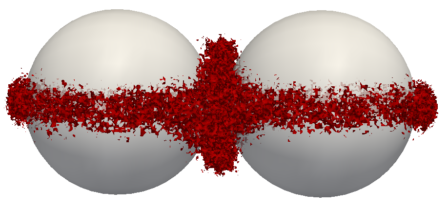
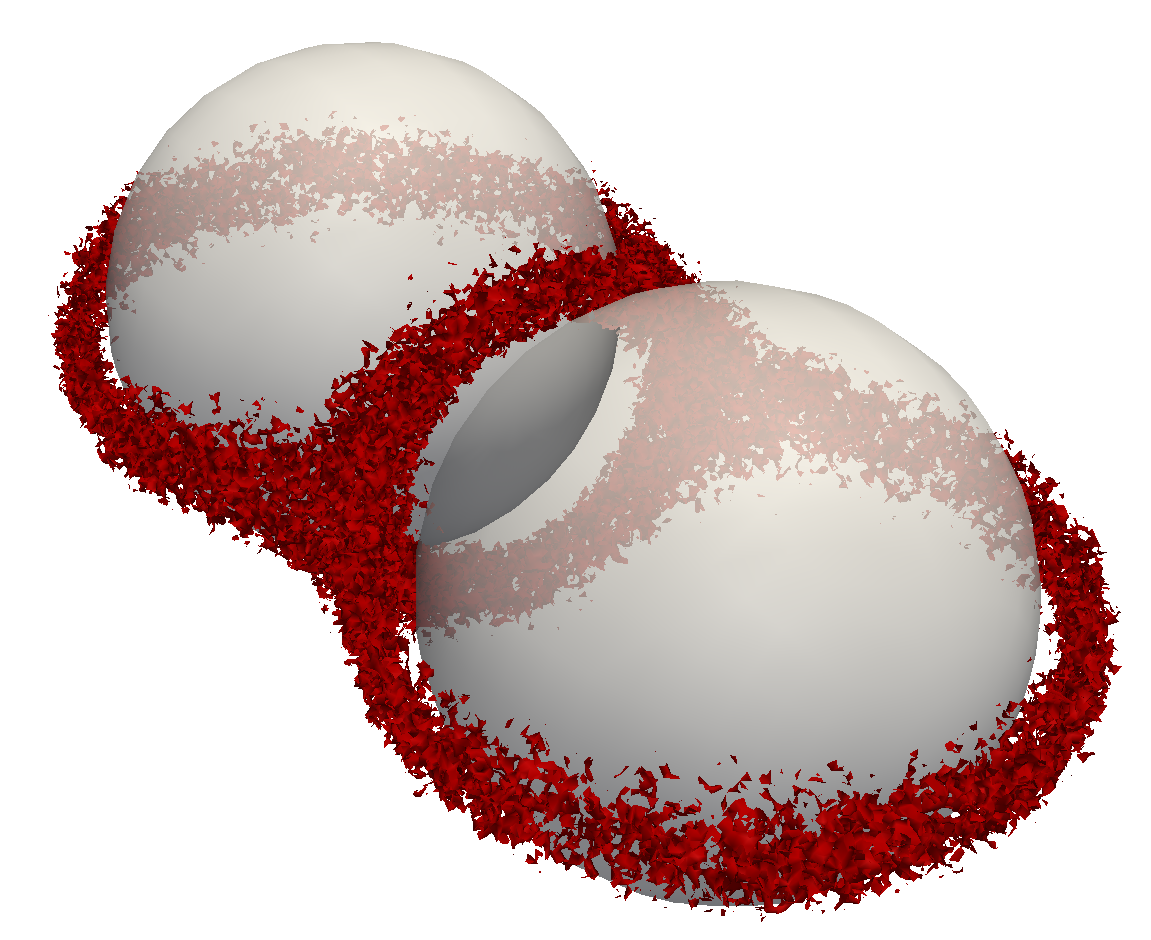
Figure 7: Disclination line (red) corresponding to $S<0.4$ time-averaged over entire production run for $R_{\text{NP}}=10\sigma_{0}$ and $\Delta=2.94\sigma_{0}$

The time-averaged disclination line forms the three-ring structure with two nodes previously observed. It appears that it is a product of the frequent transitions and not a stable defect structure itself. We do not observe such a structure in any instantaneous snapshot. It appears that the visualisation technique here is important: the common approach using small bins is inadequate to capture the fast fluctuations. Using a weighted order tensor including several neighbouring molecules on a fine grid has proven itself as a very accurate method to locate defect regions.

Our results are in good agreement with calculations by Araki et al. Araki and Tanaka (2006); Araki et al. (2013), who observed the figure of eight for nanoparticles using numerical methods based on nematodynamics. In addition we have observed the figure of omega and figure of theta for the first time in molecular simulations.

The results suggest that the entanglement for nanoparticles of sizes studied here is too weak to observe stable entangled defects, given that the defects frequently transition between different states and often form intermediate structures which we expect to be highly unstable. Future work should address larger particle inclusions to generate more stable defect structures; this could be achieved using the techniques described in Section II. Whether a molecular simulation could access the longer length scales necessary to observe transitions between stable entangled defects remains to be seen.

V Conclusions

Molecular simulations were successfully used to simulate defects around two spherical nanoparticles in close vicinity in a nematic host. In our exploratory simulations we studied three different radii and several different surface-to-surface separations. Five different defect structures formed: well-separated Saturn rings, the figure of eight, the figure of omega, the figure of theta and an intermediate structure. To our knowledge this is the first observation of the figure of omega and figure of theta for nanoparticles. The observation of intermediate structures was due to the small size of the particle inclusions as well as simulations allowing access to much smaller time scales than experiments. All defect structures observed were qualitatively similar to observations made for micron-sized particles; however for the particle sizes studied here the transitions were very fast and none of the entangled structures persisted for more than a few hundred time steps. This suggests that very small particles cannot be effectively bound together by entangled lines and that thermal energies are higher than the energy barriers between different entangled defect structures. Our analysis reveals that the three-ring structure observed in previous molecular simulations is solely an artefact of time-averaged superpositions of the different entangled states and not a stable defect structure itself.

To further explore the phenomenon of entangled nanoparticles in molecular simulations we suggest a significant increase in particle size. We expect that the transitions will occur less frequently for larger particles and hence the dynamics of the system could be studied. However one has to keep in mind that this would require much longer simulation times to study transitions. At this point we have to stress that our simulations were pushing the current limits of computing resources available. Therefore it is likely that rare event simulation methods (see e.g. (Bolhuis and Dellago, 2010; van Erp, 2012)) will have to be applied in larger simulations to explore all types of entanglement.

Appendix A The Gay-Berne potential

The potential originally suggested by Gay and Berne Gay and Berne (1981) is widely used to simulate liquid crystals. It can be regarded as a shifted, anisotropic Lennard-Jones potential, i.e. it depends on the relative orientation of the particles as well as their separation. For identical uniaxial particles it can be written as Berardi et al. (1993); Cleaver et al. (1996)

$$U(\hat{\bm{u}}_{i},\hat{\bm{u}}_{j},\bm{r}_{ij})=4\epsilon(\hat{\bm{u}}_{i},\hat{\bm{u}}_{j},\hat{\bm{r}}_{ij})\bigl{[}\varrho^{-12}-\varrho^{-6}\bigr{]}\>,$$ (4)

where

$$\varrho(\hat{\bm{u}}_{i},\hat{\bm{u}}_{j},\bm{r}_{ij})=\frac{r_{ij}-\sigma(\hat{\bm{u}}_{i},\hat{\bm{u}}_{j},\hat{\bm{r}}_{ij})+\sigma_{0}}{\sigma_{0}}\>.$$ (5)

$\hat{\bm{u}}_{i}$ and $\hat{\bm{u}}_{j}$ are unit vectors along the principal axes of the two particles $i$ and $j$, while $\bm{r}_{ij}=\bm{r}_{i}-\bm{r}_{j}$ is the vector connecting their centres of mass, $r_{ij}=|\bm{r}_{ij}|$, and $\hat{\bm{r}}_{ij}=\bm{r}_{ij}/r_{ij}$. $\sigma_{0}$ is a parameter representing the width of the particle. $\sigma(\hat{\bm{u}}_{i},\hat{\bm{u}}_{j},\hat{\bm{r}}_{ij})$ is the orientation-dependent range parameter

$$\sigma =\sigma_{0}\bigl{[}1-\tfrac{1}{2}\chi(S_{+}+S_{-})\bigr{]}^{-1/2}$$

$$\text{where}\quad S_{\pm} =\frac{\left(\hat{\bm{r}}_{ij}\cdot\hat{\bm{u}}_{i}\pm\hat{\bm{r}}_{ij}\cdot\hat{\bm{u}}_{j}\right)^{2}}{1\pm\chi\hat{\bm{u}}_{i}\cdot\hat{\bm{u}}_{j}}\>.$$

Here $\chi$ is given by $\chi=(\kappa^{2}-1)(\kappa^{2}+1)$, where $\kappa$ is the length-to-width ratio of the particle. The strength anisotropy function $\epsilon(\hat{\bm{u}}_{i},\hat{\bm{u}}_{j},\hat{\bm{r}}_{ij})$ used in Equation (4) is given by

$$\epsilon(\hat{\bm{u}}_{i},\hat{\bm{u}}_{j},\hat{\bm{r}}_{ij})=\epsilon_{0}\,\epsilon_{1}^{\nu}(\hat{\bm{u}}_{i},\hat{\bm{u}}_{j})\,\epsilon_{2}^{\mu}(\hat{\bm{u}}_{i},\hat{\bm{u}}_{j},\hat{\bm{r}}_{ij})\>.$$ (6)

$\epsilon_{0}$ is the well depth parameter determining the overall strength of the potential, while $\nu$ and $\mu$ are two adjustable exponents which allow considerable flexibility in defining a family of Gay-Berne potentials. $\epsilon_{1}$ and $\epsilon_{2}$ are given by

$$\epsilon_{1} =\left[1-\chi^{2}(\hat{\bm{u}}_{i}\cdot\hat{\bm{u}}_{j})^{2})\right]^{-1/2}\>,$$

$$\epsilon_{2} =1-\tfrac{1}{2}\chi^{\prime}(S_{+}^{\prime}+S_{-}^{\prime})$$

$$\text{where}\quad S_{\pm}^{\prime} =\frac{\left(\hat{\bm{r}}_{ij}\cdot\hat{\bm{u}}_{i}\pm\hat{\bm{r}}_{ij}\cdot\hat{\bm{u}}_{j}\right)^{2}}{1\pm\chi^{\prime}\hat{\bm{u}}_{i}\cdot\hat{\bm{u}}_{j}}\>.$$

Here

$$\chi^{\prime}=\frac{\kappa^{\prime 1/\mu}-1}{\kappa^{\prime 1/\mu}+1}\>,$$ (7)

where $\kappa^{\prime}=\epsilon_{\text{S}}/\epsilon_{\text{E}}$ is the ratio of well depths for the side-to-side configuration, $\epsilon_{\text{S}}$, and the end-to-end configuration, $\epsilon_{\text{E}}$, of two molecules.

Appendix B Homeotropic surface anchoring

Instead of using a specific anchoring potential, a simple variation of the standard Lennard-Jones (LJ) 12-6 potential is used. Here the anchoring is entirely induced by the packing effects of the liquid crystal particles near the surface of the nanoparticle. For the homeotropic surface anchoring, the Gay-Berne (GB) molecules are allowed to penetrate the surface of the nanoparticle. To prevent GB molecules from entirely entering the particle, a shifted purely repulsive LJ interaction potential $U_{\text{homeo}}$

$$U_{\text{homeo}}(\bm{r})=\left\{\begin{array}[]{ll}4\epsilon_{0}\left(\varrho^{-12}-\varrho^{-6}\right)+\epsilon_{0}&\mbox{if }\varrho^{6}<2\\ 0&\mbox{else}\end{array}\right.$$ (8)

is used. $\epsilon_{0}$ is an energy parameter chosen to be unity and $\varrho$ is given by

$$\varrho=\frac{|\bm{r}|-\sigma_{c}+\sigma_{0}}{\sigma_{0}}\>.$$ (9)

Here $\bm{r}_{ij}$ is the vector connecting the positions of the nanoparticle and the GB molecule and $\bm{\hat{r}}_{ij}$ is the corresponding unit vector. $\sigma_{0}$ is a size parameter and defined as the smallest diameter of the GB molecule; in this system $\sigma_{0}=1$. $\sigma_{c}$ is the distance of closest approach between the GB molecule and the nanoparticle, set to

$$\sigma_{c}=R_{\text{NP}}+\sigma_{0}/2\>,$$ (10)

where $R_{\text{NP}}$ is the radius of the spherical nanoparticle. For this interaction potential, the potential cutoff is chosen to be $R_{\text{NP}}+1$.

References

- Stark (2002) H. Stark, Nature 493, 200 (2002).
- Guzmán et al. (2003) O. Guzmán, E. B. Kim, S. Grollau, N. L. Abbott, and J. J. de Pablo, Phys. Rev. Lett. 91, 235507 (2003).
- Araki and Tanaka (2006) T. Araki and H. Tanaka, Phys. Rev. Lett. 97, 127801 (2006).
- Ravnik et al. (2007) M. Ravnik, M. Skarabot, S. Zumer, U. Tkalec, I. Poberaj, D. Babic, N. Osterman, and I. Musevic, Phys. Rev. Lett. 99, 247801 (2007).
- Škarabot et al. (2008) M. Škarabot, M. Ravnik, U. Tkalec, I. Poberaj, D. Babič, and I. Muševič, Phys. Rev. E 77, 061706 (2008).
- Ravnik and Žumer (2009a) M. Ravnik and S. Žumer, Soft Matter 5, 269 (2009a).
- Čopar and Žumer (2011) S. Čopar and S. Žumer, Phys. Rev. Lett. 106, 177801 (2011).
- Kim et al. (2004) E. B. Kim, O. Guzmán, S. Grollau, N. L. Abbott, and J. J. de Pablo, J. Chem. Phys. 121, 1949 (2004).
- Tkalec and Muševič (2013) U. Tkalec and I. Muševič, Soft Matter 9, 8140 (2013).
- Ravnik and Žumer (2009b) M. Ravnik and S. Žumer, Liq. Cryst. 36, 1201 (2009b).
- Grollau et al. (2003) S. Grollau, E. B. Kim, O. Guzmán, N. L. Abbott, and J. J. de Pablo, J. Chem. Phys. 119, 2444 (2003).
- Hung (2009) F. R. Hung, Phys. Rev. E 79, 021705 (2009).
- Ravnik and Žumer (2009c) M. Ravnik and S. Žumer, Soft Matter 5, 4520 (2009c).
- Araki et al. (2013) T. Araki, F. Serra, and H. Tanaka, Soft Matter 9, 8107 (2013).
- Tkalec et al. (2011) U. Tkalec, M. Ravnik, S. Čopar, S. Žumer, and I. Muševič, Science 333, 62 (2011).
- Nikkhou et al. (2015) M. Nikkhou, M. Škarabot, and I. Muševič, Euro. Phys. J. E 38, 115 (2015).
- Jampani et al. (2011) V. S. R. Jampani, M. Škarabot, M. Ravnik, S. Čopar, S. Žumer, and I. Muševič, Phys. Rev. E 84, 031703 (2011).
- Čopar et al. (2015) S. Čopar, U. Tkalec, I. Muševič, and S. Žumer, Proc. Nat. Acad. Sci. 112, 1675 (2015).
- Wood et al. (2011) T. A. Wood, J. S. Lintuvuori, A. B. Schofield, D. Marenduzzo, and W. C. K. Poon, Science 334, 79 (2011).
- Agarwal et al. (2008) A. Agarwal, E. Huang, S. Palecek, and N. L. Abbott, Adv. Mater. 20, 4804 (2008).
- Callan-Jones et al. (2006) A. C. Callan-Jones, R. A. Pelcovits, V. A. Slavin, S. Zhang, D. H. Laidlaw, and G. B. Loriot, Phys. Rev. E 74, 061701 (2006).
- Bartels et al. (1987) R. H. Bartels, J. C. Beatty, and B. A. Barsky, An introduction to splines for use in computer graphics and geometric modeling (Morgan Kaufmann, 1987).
- Cormen et al. (2001) T. H. Cormen, C. E. Leiserson, R. L. Rivest, and C. Stein, Introduction to Algorithms (MIT Press, 2001).
- Ravnik et al. (2009) M. Ravnik, B. Črnko, and S. Žumer, Mol. Cryst. Liq. Cryst. 508, 150 (2009).
- Bolhuis and Dellago (2010) P. G. Bolhuis and C. Dellago, in Rev. Comput. Chem., Reviews in Computational Chemistry, Vol. 27, edited by K. B. Lipkowitz (John Wiley & Sons, Inc., 2010) Chap. 3, pp. 111–210.
- van Erp (2012) T. S. van Erp, Kinetics and Thermodynamics of Multistep Nucleation and Self-Assembly in Nanoscale Materials, Adv. Chem. Phys. 151, 27 (2012).
- Gay and Berne (1981) J. G. Gay and B. J. Berne, J. Chem. Phys. 74, 3316 (1981).
- Berardi et al. (1993) R. Berardi, A. P. J. Emerson, and C. Zannoni, J. Chem. Soc. Faraday Trans. 89, 4069 (1993).
- Cleaver et al. (1996) D. J. Cleaver, C. M. Care, M. P. Allen, and M. P. Neal, Phys. Rev. E 54, 559 (1996).