Abstract

The analysis of high-energy particle collisions is an excellent testbed for the non-extensive statistical approach. In these reactions we are far from the thermodynamical limit. In small colliding systems, such as electron-positron or nuclear collisions, the number of particles is several orders of magnitude smaller than the Avogadro number; therefore, finite-size and fluctuation effects strongly influence the final-state one-particle energy distributions. Due to the simple characterization, the description of the identified hadron spectra with the Boltzmann–Gibbs thermodynamical approach is insufficient. These spectra can be described very well with Tsallis–Pareto distributions instead, derived from non-extensive thermodynamics. Using the $q$-entropy formula, we interpret the microscopic physics in terms of the Tsallis $q$ and $T$ parameters. In this paper we give a view on these parameters, analyzing identified hadron spectra from recent years in a wide center-of-mass energy range. We demonstrate that the fitted Tsallis-parameters show dependency on the center-of-mass energy and particle species (mass). Our findings are described well by a QCD (Quantum Chromodynamics) inspired parton evolution ansatz. Based on this comprehensive study, apart from the evolution, both mesonic and baryonic components found to be non-extensive ($q>1$), besides the mass ordered hierarchy observed in the parameter $T$. We also study and compare in details the theory-obtained parameters for the case of PYTHIA8 Monte Carlo Generator, perturbative QCD and quark coalescence models.

88 10.3390/e19030088 19 Academic Editor: Geert Verdoolaege Received: 4 February 2017; Accepted: 22 February 2017; Published: 24 February 2017 Systematic Analysis of the Non-Extensive Statistical Approach in High Energy Particle Collisions—Experiment vs. Theory ^† Gábor Bíró ^1,2,*, Gergely Gábor Barnaföldi ¹, Tamás Sándor Biró ¹, Károly Ürmössy ³ and Ádám Takács ² Gábor Bíró, Gergely Gábor Barnaföldi, Tamás Sándor Biró, Károly Ürmössy and Ádám Takács Correspondence: biro.gabor@wigner.mta.hu; Tel.: +36-30-308-6742 MaxEnt 2016 MaxEnt 2016

1 Introduction

In Nature we often meet phenomena with a large number of variables where the few-body approach breaks down. In these cases the standard procedure is to apply tools from statistical physics and inspect thermodynamical quantities of the system, instead of treating all degrees of freedom one-by-one. A certain generalization of the standard Boltzmann–Gibbs entropy is promoted by Constantino Tsallis, introducing the $q$-entropy formula, central to non-extensive statistical theory book:ts ; book:ts2 . Despite its unconventional form, in the last two decades the Tsallis-entropy was found to be a very general and descriptive notion. Numerous physical observations were successfully explained using non-extensive statistical physics book:nonextcollection ; TsallisBibHtml ; artic:tsappl1 ; artic:tsappl2 ; artic:tsappl3 . From our perspective the field of high-energy physics is especially important, since that community uses efficiently these tools to describe the results of high-energy particle and nuclear collisions. It is an experimental finding that the distributions derived from Tsallis-entropy fit the spectrum of high-energy particles, produced by many systems starting from electron-positron collisions up to the cosmic rays. In this paper we focus on identified hadron spectra, measured in proton-proton collisions. We put emphasis on the investigation of the center-of-mass energy ($\sqrt{s}$) dependence of the Tsallis parameters $q$ and $T$, assuming a Quantum Chromodynamics (QCD) inspired logarithmic scaling of these parameters. We use units in which $\hbar=c=k_{B}=1$.

The outline of the paper is the following: in the next section we enlist our motivation from high energy physics and the goals of our analysis. In Section 3 we briefly introduce the mathematical apparatus we used during our investigation. In Section 4 we show experimental results, while in Section 5 we compare them to state-of-the-art theoretical models. Finally, in Section 6 we summarize our work and give a discussion, including our future plans.

2 Connection with High Energy Physics

One of the main goals in high-energy heavy-ion physics is to understand the properties of the so-called Quark Gluon Plasma (QGP), a particular form of the strongly interacting matter which existed shortly after the Big Bang. With today’s high-energy particle accelerators we are able to reach the energy range where this superdense matter of the early Universe can be formed for a short, $\mathcal{O}$(fm/$c$)$\sim 10^{-23}$ s time. The properties of the QGP can be studied in ultra-relativistic heavy-ion collisions indirectly. Due to the nature of the strong interaction there is no way for direct observation, only signatures stemming from the final state allow us to draw conclusions. On the other hand, the reactions occur during a very short time and our information about their nature is very limited. This is a strong restraint in our possibilities, especially we cannot treat properly the description at the microscopical level. Nevertheless it is essential to understand the processes in proton-proton collisions, the baseline for heavy-ion measurements.

To date we still do not have a well established, detailed, and throughout probed theory of the hadronization, the process where the color degrees of freedom confine into hadrons. This is related to the Yang–Mills Mass Gap, one of the so-called “Millennium problems” of the Clay Mathematical Institute artic:millenium . Recent hadronization models are phenomenological, and it is quite typical that their parameters lack of any clear physical meaning.

Recently, complex detector systems, like ALICE at the Large Hadron Collider (CERN LHC) or STAR and PHENIX at the Relativistic Heavy Ion Collider (BNL RHIC) are able to measure with high accuracy the final state particles. The hadron spectra, measured in high-energy collisions, are one of the most fundamental characteristics of these events and involve both microscopic and collective effects in high-energy collisions. Identifying their most crucial problems is a key task for understanding hadronization. A remarkable phenomenon is that these properties occur not only in heavy-ion collisions, but even for small colliding systems like proton-proton or electron-positron collisions artic:flowing0 ; artic:flowing1 ; artic:flowing2 ; artic:flowing3 ; artic:gbiro .

The aim of our study is to find the common source of these similarities and to recognize the driving mechanisms behind the observations. For this aim, we built a consistent non-extensive approach, in which fit parameters carry important physical information about the observed system of high-energy and strongly interacting particles including reactions and collective effects among them.

3 Non-Extensive Statistics in High-Energy Physics

High-energy physics, and in particular high-energy heavy ion physics is an interdisciplinary topic. It uses the theory of relativistic quantum fields, statistical physics, thermo- and hydrodynamics, and even the theory of curved space-times. Earlier studies show that non-extensive statistical physics provides a useful tool to describe particle-particle collisions, where “particle” now stands either for electron/positron, or for proton or a heavy nucleus. The non-extensivity in high-energy physics manifests itself both in the non-exponential energy- and non-Poissonian multiplicity distributions.

The hadron spectra can be characterized with Tsallis–Pareto-like distributions, both at low-, and high transverse momenta very well artic:gbiro ; artic:tsbeurphys2 ; artic:cleymansphyslett ; artic:cleymansjphys ; artic:wilk1 ; artic:wilk2 ; artic:wilk3 ; artic:wilk4 ; artic:tsorig ; artic:wilkentr ; artic:actaphys ; artic:chaossolitions . The origin of these distributions lies in the assumption that subsystems are not independent of each other. It makes them a good candidate to investigate the QGP in heavy ion collisions or the baseline in smaller colliding systems. Recently a number of systematic analyses have been made in order to find the best form for these distributions artic:lilin1 ; artic:lilin2 ; artic:cleymansTS ; artic:cleymansqspecies ; artic:flowing0 ; artic:flowing1 ; artic:flowing2 ; artic:flowing3 , but in this present study we compare theoretical and experimental results in a wide energy range comprehensively.

3.1 The Description of the Inclusive Hadron Production

The Quantum Chromodynamics is the fundamental theory of the strong interaction. Due to the energy-scale dependent behavior of the strong coupling, the perturbative QCD (pQCD) based parton model–initiated by Bjorken and Feynman–works extremely well at high energies artic:bjorken . In the framework of the pQCD-based parton model, all hadrons are made up from partons (bare, nearly massless quarks and gluons), therefore the inner structure of the initial colliding and the finally produced hadrons are described by the parton distribution functions (PDF) and by the fragmentation functions (FF), respectively. These non-perturbative distribution functions are defined in the momentum space and can be parametrized by a polynomial ansatz. The PDF,

$$f_{a/h}(x_{a},Q^{2})\ \ ,$$ (1)

gives the distribution of parton $a$ inside the hadron $h$ at the energy scale, $Q^{2}$, while $x_{a}=p_{a}/p_{h}$ is the momentum fraction carried by that parton. On the other hand, the confinement of the parton $c$ into the final state hadron $h$ with the momentum fraction $z_{c}=p_{h}/p_{c}$ can be described at scale, $\tilde{Q}^{2}$ with the help of fragmentation functions

$$D_{c}^{h}(z_{c},\tilde{Q}^{2}).$$ (2)

In this framework the inclusive cross-section of a given hadron $h$ produced in proton-proton collisions can be calculated by the following convolution:

$$E_{h}\frac{{\textrm{d}}^{3}\sigma_{h}^{pp}}{{\textrm{d}}p_{h}^{3}}\sim\sum\limits_{a,b,c}f_{a/p}(x_{a},Q^{2})\otimes f_{b/p}(x_{b},Q^{2})\otimes\frac{{\textrm{d}}\sigma^{ab\rightarrow cd}}{{\textrm{d}}\hat{t}}\otimes\frac{D_{c}^{h}(z_{c},\tilde{Q^{2}})}{\pi z_{c}^{2}}\ \ \ .$$ (3)

Here the parton distribution function of a proton is denoted by $f_{a/p}(x_{a},Q^{2})$ and $\frac{{\textrm{d}}\sigma}{{\textrm{d}}\hat{t}}$ is the differential cross-section of the $ab\rightarrow cd$ partonic process, the variable $\hat{t}$ is related to the 4-momentum exchange of the particles.

The hadronization is described within the parton model by the above phenomenological fragmentation functions, for which several forms of parametrization exist in the literature. These parametrizations are usually fitted to lepton scattering data, therefore they describe existing experimental results in a broad-range in the parameter space. In Section 5, after investigating the energy dependence, we show the latest results of a new fragmentation function parametrization based on non-extensive phenomena.

3.2 Hadronization Using Non-Extensive Statistics

As we have already mentioned, the transverse energy distribution of the measured hadrons—the particle yield measured in the $y\in[-0.5,+0.5]$ midrapidity region–is an important quantity accessible to measurement. In practice, the low-energy regime is described by exponential-like functions, as a thermalized system, while the high $p_{T}$ regime behaves like a power-law, $p_{T}^{-n}$. The Tsallis–Pareto-like distributions handle these two regimes simultaneously.

The technical apparatus in the high-energy physics shows a great advancement, nowadays the statistics of these spectra is larger than ever. It is no surprise that the Tsallis–Pareto distributions are widely used by the high-energy community to describe hadron spectra. The STAR and PHENIX collaborations at RHIC BNL (USA) and the European CERN’s ALICE, ATLAS, and CMS collaborations at the LHC are using the following form to characterize the particle yield artic:phenixts ; artic:starts ; artic:62gevphenix ; artic:097tevalice ; artic:cmsts ; artic:atlasts :

$$\frac{1}{2\pi p_{T}}\frac{{\textrm{d}}^{2}N}{{\textrm{d}}y{\textrm{d}}p_{T}}=\frac{{\textrm{d}}N}{{\textrm{d}}y}\frac{(n-1)(n-2)}{2\pi nC\left(nC+m(n-2)\right)}\left(1+\frac{m_{T}-m}{nC}\right)^{-n}\ \ \ ,$$ (4)

where $n$ and $C$ are fit parameters and $m_{T}=\sqrt{p_{T}^{2}+m^{2}}$ is the transverse mass, including the rest mass $m$ of the given identified hadron species. We note that this formula is based on the QCD-Hagedorn formula artic:qcdhagedorn ; artic:ua1hagedorn1 ; artic:ua1hagedorn2 ; artic:mpprod1 ; artic:mpprod2 . This and other variations of the distribution are exhaustively tested e.g., in artic:gbiro ; artic:tsbeurphys2 ; artic:flowing0 ; artic:flowing1 ; artic:flowing2 ; artic:flowing3 ; artic:cleymansphyslett ; artic:lilin1 ; artic:lilin2 . Below we theoretize over the origin of such Tsallis-type formulas. Contrary to the fixed fit parameters of the Tsallis–Pareto distributions as in Equation (4), we assume that the identified hadron spectra are characterized with a scaling Tsallis-distribution, where an energy scaling of the Tsallis-parameters is also present. In the following we refer to these as Tsallis-like distributions.

In extensive systems the entropy is finite in the thermodynamical limit, $\lim\limits_{N\rightarrow\infty}\frac{S_{N}}{N}<\infty$. This is the case with the Boltzmann–Gibbs–Shanon entropy formula, $S=-\sum\limits_{i}P_{i}\ln{P_{i}}$, where $P_{i}$ is the probability of being in state $i$. In strongly correlated systems, it turns out that the total entropy of the system is not the sum of the entropy of the subsystems:

$$S_{12}\neq S_{1}+S_{2}\ \ .$$ (5)

For our generalization, we use the well established terminology of the thermodynamics, since we expect to include the classical Boltzmann–Gibbs case too. Let us consider a monotonic, transformed entropy, $L(S)$, which satisfies additivity ,

$$L(S_{12})=L(S_{1})+L(S_{2})\ .$$ (6)

Note, on general terms $L(S)$ is the logarithm of the formal group of phase space factors $\Omega(S)=e^{S}$. Due to this assumption, applied recursively in ensembles, we arrive at the following general class of entropies artic:tsbentr :

$$L(S)=\sum\limits_{i}P_{i}L(-\ln{P_{i}})\ \ \ .$$ (7)

Because $L(S)$ is by definition a monotonic function, the most likely state of a heat reservoir and its subsystem at maximum entropy is equivalently at

$$L\left(S_{1}(E_{1}^{*}\right))+L\left(S_{2}(E_{2}^{*})\right)=\mathrm{max}\ \ \ ,$$ (8)

where $E_{1}$ is the energy of the subsystem, $E_{2}=E-E_{1}$ is the energy of the reservoir. While keeping $E~{}=~{}$const in the entropy maximum Equation (8) we obtain

$$0=\left.\frac{\partial L}{\partial S_{1}}\right|_{S_{1}(E_{1}^{*})}\times\left.\frac{\partial S_{1}}{\partial E_{1}}\right|_{E_{1}^{*}}-\left.\frac{\partial L}{\partial S_{2}}\right|_{S_{2}(E_{2}^{*})}\times\left.\frac{\partial S_{2}}{\partial E_{2}}\right|_{E_{2}^{*}}\ \ \ .$$ (9)

It makes the use of the usual definition of thermodynamical temperature expedient,

$$\beta_{1}:=\left.\frac{\partial L}{\partial S_{1}}\right|_{S_{1}(E_{1}^{*})}\times\left.\frac{\partial S_{1}}{\partial E_{1}}\right|_{E_{1}^{*}}=\left.\frac{\partial L}{\partial S_{2}}\right|_{S_{2}(E_{2}^{*})}\times\left.\frac{\partial S_{2}}{\partial E_{2}}\right|_{E_{2}^{*}}=\beta_{2}\ \ \ .$$ (10)

Assuming now $E_{1}\ll E$ in high-energy collisions, we consider: $E\rightarrow\sqrt{s}$ and $E_{1}\rightarrow(m_{T}-m)\approx p_{T}$ of the particle,

$$L(S_{2}(E-E_{1}))\approx L\left(S_{2}(E)-\left.\frac{\partial S_{2}}{\partial E_{2}}\right|_{E}\times E_{1}\right)\approx L(S_{2}(E))-\left.\frac{\partial L}{\partial S_{2}}\right|_{S_{2}(E)}\times\left.\frac{\partial S_{2}}{\partial E_{2}}\right|_{E}\times E_{1}\ \ .$$ (11)

Inserting this into Equation (10), we arrive at the formula,

$$\beta_{1}\approx\left.\frac{\partial L}{\partial S_{2}}\right|_{S_{2}(E)}\times\left.\frac{\partial S_{2}}{\partial E_{2}}\right|_{E}-\left[\left.\frac{\partial^{2}L}{\partial S^{2}_{2}}\right|_{S_{2}(E)}\times\left(\left.\frac{\partial S_{2}}{\partial E_{2}}\right|_{E}\right)^{2}+\left.\frac{\partial L}{\partial S_{2}}\right|_{S_{2}(E)}\times\left.\frac{\partial^{2}S_{2}}{\partial E^{2}_{2}}\right|_{E}\right]\times E_{1}+\dots\ \ .$$ (12)

By looking for an universal termostat, lending to $\beta_{1}$ an absolute temperature interpretation, we assume that the energy of the subsystem is independent from the energy of the reservoir, i.e., we require the term linear in $E_{1}$ to vanish. After ordering we obtain:

$$\left.\left.\frac{\partial^{2}L}{\partial S^{2}_{2}}\right|_{S_{2}(E)}\right/\left.\frac{\partial L}{\partial S_{2}}\right|_{S_{2}(E)}=-\left.\left.\frac{\partial^{2}S_{2}}{\partial E^{2}_{2}}\right|_{E}\right/\left(\left.\frac{\partial S_{2}}{\partial E_{2}}\right|_{E}\right)^{2}\ \ \ .$$ (13)

This equality among general functions, $L(S)$ and $S(E)$ is possible only if both are equal with a constant,

$$\frac{L^{\prime\prime}(S)}{L^{\prime}(S)}=-\frac{S^{\prime\prime}(E)}{S^{\prime}(E)^{2}}=\frac{1}{C}:=1-q\ ,$$ (14)

where $C$ is the heat capacity of the reservoir.

The solution of this differential equation has all desired features:

$$L(S)=\frac{{\textrm{e}}^{(1-q)S}-1}{1-q}\ \ \ .$$ (15)

Replacing it into the Equation (7),

$$L(S)=\sum\limits_{i}P_{i}\frac{{\textrm{e}}^{-(1-q)\ln P_{i}}-1}{1-q}=\frac{1}{1-q}\sum\limits_{i}P_{i}\left(P_{i}^{q-1}-1\right)=\frac{1}{1-q}\sum\limits_{i}\left(P_{i}^{q}-P_{i}\right)$$ (16)

is the (now additive) Tsallis entropy, while

$$S=\frac{1}{1-q}\ln\left(1+(1-q)L(S)\right)=\frac{1}{1-q}\ln\sum\limits_{i}P_{i}^{q}\ \ ,$$ (17)

turns out to be the Rényi entropy.

This argumentation can be used also for microcanonical systems, with $S_{1}=-\ln{P_{1}}$ and $P_{1}$ being the distribution of the subsystem’s states. Using the previously-defined generalized entropy, $L(S)$, one arrives at the following energy distribution, which maximizes the $q$-entropy:

$$P_{i}=\left(Z^{1-q}+(1-q)\frac{E_{i}}{T}\right)^{-\frac{1}{1-q}}\ \ \ .$$ (18)

It is a Tsallis–Pareto distribution with the individual energy, $E_{i}$ and $Z$ is calculated form $\sum p_{i}=1$.

In high-energy collisions we also have to deal with fluctuations event by event. Following the calculations in references artic:tsbentr ; artic:tsbphysica , one may assume that the multiplicity of the created hadrons follow a negative-binomial distribution for bosons, a binomial one for fermions. Due to such general reservoir fluctuations, the $q$ non-extensivity parameter receives a correction artic:tsbentr ; artic:tsbphysica :

$$q=1-\frac{1}{C}+\frac{\Delta\beta^{2}}{\left<\beta\right>^{2}}\ \ \ .$$ (19)

As the average number of created particles can vary in a wide range depending on the studied system–typically $\mathcal{O}(10^{2})$ in proton-proton collisions, while $\mathcal{O}(10^{3}-10^{5})$ in nucleus-nucleus collisions. We expect this fluctuation effect to overcome the finite heat capacity condition, therefore one observes $q>1$. It is also straightforward to see that enlarging the system results in $C\to\infty$, and if fluctuations become sufficiently suppressed, we get back the Boltzmann–Gibbs case with exponential distribution. On the other hand, the assumption $q\rightarrow 1$ leads to a Gaussian distribution for the $\beta$ values, which can be an approximation, but never the complete truth. This parameter is used to call the entropic index or the non-extensivity parameter, present as a measure of the deviation from the Boltzmann–Gibbs case, $q=1$. We note, in high-energy nuclear collisions this value is in the range $1.0<q<1.5$, which suggests fluctuations override the system size effects, related to the heat capacity of the reservoir.

The distributions Equations (4) and (18) behave similarly, they both can be regarded as Tsallis–Pareto-type distributions. The authors in artic:lilin1 ; artic:lilin2 investigated how the different types fit the experimental data. Many further useful readings regarding the thermodynamically consistent non-extensive approach can be found in the literature. The first possibility is presented in artic:wilkentr ; artic:actaphys ; artic:chaossolitions , representing the case where the power is proportional to $\frac{1}{q-1}$. An another kind of approach where the power is $\frac{q}{1-q}$, as discussed in references artic:tsthermo1 ; artic:tsthermo2 ; artic:tsthermo3 ; artic:tsthermo4 . For our analysis the chosen form is the following book:tsb :

$$\left.\frac{1}{N_{ev}}\frac{{\textrm{d}}^{2}N}{2\pi p_{T}{\textrm{d}}p_{T}{\textrm{d}}y}\right|_{y\approx 0}=A\times\left[1+\frac{q-1}{T}(m_{T}-m)\right]^{-\frac{1}{q-1}}\ \ \$$ (20)

As it was shown in artic:tsbphysica ; artic:tsbphysica2 the parameters $q$ and $T$ for an ideal case are connected to the mean multiplicity and its variance:

$$T=\frac{E}{\left<N\right>},\ \ \ \ \ q=\frac{\left<N(N+1)\right>}{\left<N\right>^{2}}\ \ \ .$$ (21)

They also may depend on each other. Since in case of $q\to 1$ one has $T\to T_{BG}$, the parameter $q$ is a measure of non-extensitivity (i.e., non-Gaussivity in $\beta$ fluctuations, non-Poissonity in the multiplicity distribution $P(N)$). $T$ is like the kinetic temperature.

Based on Equation (21), for fixed $\Delta N^{2}/\left<N\right>^{2}=\sigma^{2}$ one obtains:

$$\frac{T}{E}=\sigma^{2}+(1-q)\ \ \ .$$ (22)

On the other hand for an NBD (Negative Binomial Distribution) with fixed $\left<N\right>/k=f$ one gets

$$T=E\times f\times(q-1)\ \ \ .$$ (23)

Our aim in the followings is to explore the center-of-mass energy evolution of the parameters $q$ and $T$, especially keeping in our mind their physical meaning. Based on the definition of the PDF and FF of the pQCD-based parton model, we expect a logarithmic scaling. Since this was observed even in fits of electron-positron data artic:flowing0 , where PDFs do not appear, we connect the non-extensive features with the hadronization (fragmentation) processes only. The argumentation behind this will be explained in the next subsection.

3.3 Motivation for Qcd-Like Energy Scaling of the Parameters

Partons, the elementary momentum carriers in the strongly interacting matter, are tagged with a quantum number named color, which property is not observable directly. The quarks, antiquarks and gluons together confine into color singlet hadrons during the hadronization process. Hadron formation can happen at any energy scale, $Q^{2}$. The dependency on it can be factorized into the running nature of the strong interaction’s coupling constant, $\alpha(Q^{2})$. Since any observable quantity should be independent of the arbitrary fixing of the energy scale appearing in perturbative QCD calculations, the mathematical description ought to be (energy-)scale independent at any fixed order. To satisfy this request is not an easy task, due to the non-perturbative nature of non-Abelian fields at low-energy.

As we presented the hadron production within the pQCD-based parton model in Section 3.1, the convolution in Equation (3) includes the scale parameter ($Q^{2}$) in its kernel. However, the cross-section—being an observable quantity—should be independent of this inner parameter. Technically, this is achieved with the following method: while calculating the partonic (color) cross sections at a given order, the scale can be factorized out and merged into the non-perturbative phenomenological functions. These are the parton distribution and fragmentation functions, and they must satisfy a proper scale evolution equation for avoiding scale-dependent hadronic yields.

To obtain the scale invariance, the following formula should be fulfilled at any fixed order for any generic form of such phenomenological functions artic:dglap1 ; artic:dglap2 ; artic:dglap3 :

$$\frac{\partial}{\partial\ln{Q^{2}}}R(z,Q^{2})=0\ \ \ ,$$ (24)

where $R(z,Q^{2})$ can be either the PDF or FF, typically at the momentum fraction of the mother and daughter particles, $z$. In general, this evolution equation determines the possible form of quantity $R$, which naively depends on the current energy scale at a given fixed order. Solving this Callan–Symanzik equation one can obtain the energy scale dependence of the running coupling at a given order in any theory artic:pdg .

In the perturbative QCD based parton model, the parametrized parton distribution and fragmentation ansatz functions are typically given in a power-law form artic:ellis . One can get then the proper scale evolution by solving the Doksitzer–Gribov–Lipatov–Altarelly–Parisi (DGLAP) equations artic:dglap1 ; artic:dglap2 ; artic:dglap3 . Due to its polynomial power-law form, the predictive power of the calculations gets weaker at low-$z$. We expect that a Tsallis-like distribution with the appropriate parameter evolution can resolve this problem, providing a better description. This motivates us to fit $q$ and $T$ parameters as a function of the center-of-mass energy $Q^{2}\sim\sqrt{s}$ in a similar fashion, as it was done in reference artic:gribov80 . Here our aim is to test the validity of this approach via investigating the energy-evolution dependence of the parameters.

3.4 The Improved Quark-Coalescence Model

Another description of the hadron formation is based on the constituent quark scaling. In the quark coalescence model the usual underlying assumption is that the hadronization takes place in a thermal system, where all the participating partons emerge at the same temperature artic:tsbeurphys ; artic:coalescence1 . This idea was developed for the description of hadron production in high-energy heavy-ion collisions, where the bulk of the hadron yield closely follows the exponential shape. In larger colliding systems, like in central collisions of large nuclei, this idea worked well, especially for the low transverse momentum regime, $p_{T}$ < 3–5 GeV/$c$, with a single temperature parameter.

In the original approach the energy distribution of the partons follow the Boltzmann–Gibbs statistics. Then, one approximates the formation rate as the multiplication of $k$ such Boltzmann–Gibbs distributions:

$$P_{k}=\left[f_{BG}(E/k)\right]^{k}=A^{\prime}e^{-\beta E}\ \ \ .$$ (25)

In the present non-extensive framework we still assume that the partons are part of a simple ensemble, but we replace the Boltzmann–Gibbs exponentials by Tsallis–Pareto distributions. Now the rate is the following:

$$P_{k}=\left[f_{Ts}(E/k)\right]^{k}=A^{k}\left[1+\frac{q-1}{T}E_{k}\right]^{-\frac{k}{q-1}}=A^{\prime}\left[1+\frac{q^{\prime}-1}{T}E\right]^{-\frac{1}{q^{\prime}-1}}\ \ \ ,$$ (26)

with $(q^{\prime}-1)=\frac{(q-1)}{k}$. In order to test this model, we check the fitted $q$ parameters of the identified hadrons. If the equal-energy quark-coalescence theory is correct for both the quark-antiquark containing mesons and triple (anti)quark (anti)baryons, then one observes:

$$(q_{quark}-1)=2(q_{meson}-1)=3(q_{baryon}-1)\ \ \ .$$ (27)

The meson-baryon ratio for the Tsallis parameters should be around 3/2:

$$\frac{q_{meson}-1}{q_{baryon}-1}=\frac{3}{2}\ .$$ (28)

This idea formulated by Equation (28) can be tested as fitting the hadron spectra and investigating the ratio of the parameter $(q_{i}-1)$ for different identified hadron species. As the constituent quark scaling is getting stronger at larger energies, we expect to reach this theoretical value only asymptotically.

4 Fitted Parameters

For our analysis we use identified hadron spectra datasets measured in proton-proton collisions in recent years artic:62gevphenix ; artic:62gevphenix2 ; artic:200gevphenix ; artic:500gevphenix ; artic:200gevstar ; artic:097tevalice ; artic:09tevalice ; artic:276tevalice ; artic:276tevpi0alice ; artic:7tevalice ; artic:7tevalice2 . The numerical fits of the various datasets were made utilizing the CERN Root analysis software (blackhttps://root.cern.ch/blue, version 6.06/00). Although we conducted a comprehensive study, it is worth to note that it is not necessarily meaningful to compare the fit-parameter values for all existing data, because kinematical ranges may vary and the multiplicity-classes are also not defined evenly. This especially holds for kaons and protons at high $p_{T}$; this generates some uncertainty in those fits. To circumvent these difficulties, we fixed a recipe for the fit procedure making it consistently insensitive to the fit program(s), the size of the fit parameter space and input parameters.

In order to counterbalance the effect of varying ranges we perform the fit procedure in multipl steps:

1. fit of the high-$p_{T}$ part by fixing $T$ and changing $q$;

2. fit of the low-$p_{T}$ part by fixing $q$ and changing $T$;

3. fit of the whole $p_{T}$ range with both parameters, starting from the above obtained $q$ and $T$.

We define “low-$p_{T}$” as $p_{T}<4$ GeV/$c$ and the “high-$p_{T}$” part as $p_{T}\geq 2$ GeV/$c$, respectively. The overlap is intended. In the function defined in Equation (20) the parameter $T$ sets the characteristic $p_{T}$ scale. In fact, for $q\longrightarrow 1$ one obtains $f_{1}(m_{T})=Ae^{-(m_{T}-m)/T}$. The parameter $q$ on the other hand is linked to the ’power-law like’ tail at high $p_{T}$. The procedure was evaluated by comparing the $\chi^{2}/NDF$ values.

The investigated spectra and the fitted Tsallis–Pareto functions are shown in Figure 1. Upper panels of the plots present the fits of experimental data measured in proton-proton collisions at $\sqrt{s}=62.4$ GeV, 200 GeV, 500 GeV, 900 GeV, 2.76 TeV, and 7 TeV center-of-mass energies. We considered various neutral, charged and charge-averaged hadron species, $\pi^{\pm}$, $\pi^{0}$, $K^{\pm}$, $p$, and $\bar{p}$. Identified hadron $m_{T}$ spectra are scaled by constant factors ($2^{n}$) for better visibility, as indicated in the panels.

In the lower panels “Data/Fit” plots are presented for each case. One can observe how well the distribution (20) describes the yields in the whole 62.4 GeV $\leq\sqrt{s}\leq 7$ TeV center-of-mass energy range in the $m_{T}\lesssim 20$ GeV region. Within the mid $m_{T}$-regime the overlap with data is excellent, while at the highest $m_{T}$ values or for heavier hadrons the deviation is somewhat larger.

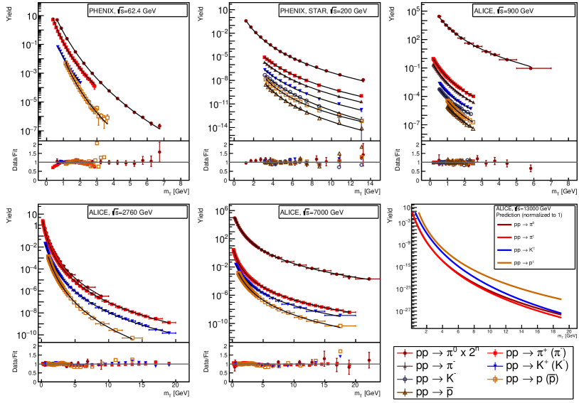
Figure 1: Upper panels are the identified hadron spectra as the function of the transverse mass, $m_{T}$ is plotted, measured by the PHENIX (artic:200gevphenix, ; artic:62gevphenix, ; artic:62gevphenix2, ; artic:500gevphenix, ), STAR (artic:200gevstar, ), and ALICE (artic:097tevalice, ; artic:09tevalice, ; artic:276tevalice, ; artic:276tevpi0alice, ; artic:7tevalice, ; artic:7tevalice2, ) at different center-of-mass energies from 62.4 GeV $\leq\sqrt{s}\leq 7$ TeV. Experimental data is in comparison with the fitted Tsallis–Pareto functions is indicated as solid lines. The $m_{T}$ spectra were scaled by constant factors ($2^{m}$) for the better visibility as indicated on the graphs. Lower panels are present the Data/Fit ratio plots including the estimated fit errors.

To determine the center-of-mass energy dependence, we review the $\sqrt{s}$ evolution of the fitted $q_{i}$ and $T_{i}$ parameters for each hadron species, $i\in~{}\left\{\pi^{\pm},\pi^{0},K^{\pm},p,\textrm{and }\bar{p}\right\}$. According to the formula (20), the parameters of the Tsallis–Pareto distribution are plotted in Figure 2 as a function of $\sqrt{s}$. Based on the motivation presented in Section 3.3, we assumed an energy-evolution for each hadron type $i$ as follows artic:karesz :

$$q_{i}(\sqrt{s})=q_{1i}+q_{2i}\log\left(\sqrt{s}/m_{i}\right),$$ (29)

$$T_{i}(\sqrt{s})=T_{1i}+T_{2i}\log\left(\sqrt{s}/m_{i}\right).$$ (30)

In these formulae, the mass $m_{i}$ of the identified hadron $i$ is used to set the physically relevant energy scale. In Equation (30) the parameter $T_{1,i}$ is fixed at $T_{1,i}=50$ MeV, as suggested by reference artic:tsbeurphys2 . Hence, the function in Equation (30) is parametrized by $T_{2,i}$.

In Figure 2a, the fitted $q_{i}$ values are plotted for each $\sqrt{s}$, for given identified hadron spectra summarized in Table 1. One can see in the graphs, that the $q_{i}(\sqrt{s})$ values are close to each other and all curves slightly increase with $\sqrt{s}$, following nicely the formula (29). For pions and kaons the increase is very similar and their evolutions are alike. However, the precise increase seems to be larger for the kaons.

We note, that charged and neutral pion results should be consistent. Taking $\pi^{0}$ and $\pi^{\pm}$ together for the fits, the mesonic components overlap more. This alternative behavior is thought to be the effect of different kinematical ranges. See more on fitted parameters and $\chi^{2}/NDF$ in Table A1 and on kinematical ranges in Table A2 in the Appendixes A and B.

Hadron, $i$	$m_{i}$	$q_{1i}$	$q_{2i}$	$T_{1i}$	$T_{2i}$
$\pi^{0}$	135.0 MeV	$1.03\pm 0.002$	$0.011\pm 0.002$	50 MeV	$0.006\pm 0.001$ MeV
$\pi^{\pm}$	140.0 MeV	$1.04\pm 0.01$	$0.009\pm 0.002$	50 MeV	$0.009\pm 0.001$ MeV
$K^{\pm}$	493.0 MeV	$1.00\pm 0.01$	$0.016\pm 0.001$	50 MeV	$0.018\pm 0.001$ MeV
$p(\bar{p})$	938.0 MeV	$1.09\pm 0.01$	$0.004\pm 0.001$	50 MeV	$0.021\pm 0.001$ MeV

Table 1: The $\sqrt{s}$-evolution of the parameters of the fitted Tsallis–Pareto distributions for hadrons, $i\in$ $\pi^{\pm}$, $\pi^{0}$, $K^{\pm}$, $p$, and $\bar{p}$ in the $62.4$ GeV $\leq\sqrt{s}\leq 7$ TeV c.m. energy range.

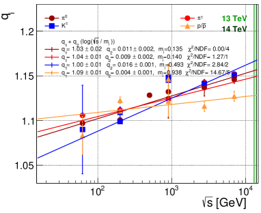
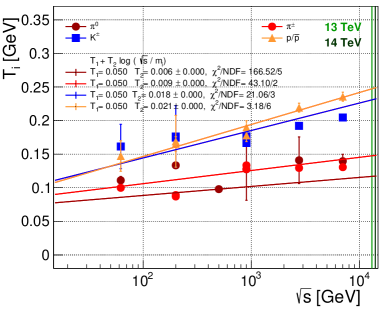
(a)	(b)

Figure 2: The fitted $q_{i}$ (a) and $T_{i}$ (b) as a function of $\sqrt{s}$ for hadron species, $i$ marked as points. Only the species of the particles are indicated. The solid color lines are fitted to the pion, kaon, and (anti)proton points. Vertical lines indicate the place of the $\sqrt{s}=13$ TeV and $14$ TeV data.

Figure 2b presents the evolution of the parameter $T_{i}$ with the center of mass energy. We applied an evolution according to $\sim\log(\sqrt{s})$ in the Figure 2 using Formula (30) with the evolution parameters listed in Table 1. Here the energy evolution of the parameter $T(\sqrt{s})$ shows an increasing trend with the mass of the hadron species. The obtained parameter values supports the idea of a mass hierarchy effect: the higher the mass, $m_{i}$, the larger $T_{2i}$.

One can realize from Figure 2a,b, by comparing them in the $\sqrt{s}<3$ TeV regime, that massive protons and kaons present the smaller change in $q_{i}$, and their masses are closer to the lattice QCD crossover temperature $T\approx 170$ MeV Katz . Light pions deviate more as increasing the energy, and the obtained $T_{\pi}$ is smaller, around $\approx 100$ MeV. It is consistent with our picture that, lighter particle can suffer larger fluctuations, which increases the parameter $q_{i}$ following Equation (19).

Based on the $\sqrt{s}$ evolution of the experimental fit curves in Figure 2, we could predict the parameter values for the soon-to-be available LHC-energy collisions at $\sqrt{s}=13$ TeV and $14$ TeV. These energies are indicated on both panels with vertical lines. According to the the assumptions given by the ansatz Formulae (29) and (30) and the fit parameters from Table 1 we summarized these values in Table 2 for $\sqrt{s}=13$ TeV. These data were used to plot the 13 TeV center-of-mass energy prediction on the bottom right panel of Figure 1. Note, $\sqrt{s}=14$ TeV data is expected to have very similar values within errors.

In Figure 3 we show the fitted $q_{i}$ and $T_{i}$ values for different hadron species at the center-of-mass energy values listed above. In agreement with reference artic:cleymansqspecies , we observe that the non-extensivity parameter $q_{i}$ on Figure 3a is less sensitive to the hadron mass, however the importance of the center-of-mass energy of the colliding system is remarkable. As we have seen already on Figure 2, pions have somewhat larger non-extensitivity than more massive hadrons:

$$q_{\pi}(\sqrt{s})\ \gtrsim\ q_{K}(\sqrt{s})\ \gtrsim\ q_{p}(\sqrt{s})\ \ \ .$$ (31)

Figure 3 also highlights that protons present weaker c.m. energy dependence than mesons.

The parameter $T_{i}$ reflects an opposite mass-hierarchy ordering, on Figure 3b. The more massive hadron, the larger $T_{i}$ value:

$$T_{\pi}(\sqrt{s})\ <\ T_{K}(\sqrt{s})\ <\ T_{p}(\sqrt{s})\ \ \ .$$ (32)

Nevertheless, we observe only a weak center-of-mass energy dependence.

Hadron, $i$	$m_{i}$	$q_{i}$	$T_{i}$ (MeV)
$\pi^{0}$	135.0 MeV	$1.156\pm 0.001$/$1.157\pm 0.001$	$119.0\pm 2.0$/$119.0\pm 2.0$
$\pi^{\pm}$	140.0 MeV	$1.143\pm 0.001$/$1.144\pm 0.001$	$153.0\pm 2.0$/$154.0\pm 2.0$
$K^{\pm}$	493.0 MeV	$1.163\pm 0.002$/$1.164\pm 0.002$	$233.0\pm 2.0$/$234.0\pm 2.0$
$p(\bar{p})$	938.0 MeV	$1.128\pm 2.0.003$/$1.128\pm 0.003$	$250.0\pm 2.0$/$252.0\pm 2.0$

Table 2: Predictions for the Tsallis–Pareto parameters for $\sqrt{s}=13$ TeV (left) and $14$ TeV (right), for hadrons $i\in$ $\pi^{\pm}$, $\pi^{0}$, $K^{\pm}$, $p$, and $\bar{p}$, based on the Formulae (29) and (30).

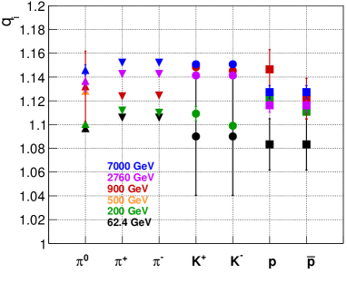
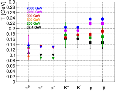
(a)	(b)

Figure 3: The fitted $q_{i}$ (a) and $T_{i}$ (b) values for each hadron type, $i\in$ $\pi^{\pm}$, $\pi^{0}$, $K^{\pm}$, $K_{s}^{0}$, $p$, and $\bar{p}$, c.f. artic:cleymansqspecies

.

4.1 The $(T,q)$ Parameter Space for Identified Hadrons

Summarizing our obserations we can conclude that the center-of-mass energy evolution of the fit parameters works well with our logarithmic evolution ansatz.

• The $q_{2i}$ and $T_{2i}$ parameters are getting slightly larger with the larger hadron mass, $m_{i}$, and applying Formulae (29) and (30) the evolution is described nicely in the whole tested energy range, $62.4$ GeV $\leq\sqrt{s}\leq 7$ TeV.

• The obtained $q_{i}(\sqrt{s})$ function increases with $\sqrt{s}$ in the range 1.07–1.17 indicating the deviation from the Boltzmann–Gibbs case where $q=1$. The deviation from this “thermodynamical limit” case grows as the center-of-mass energy gets higher values. However large statistical errorbars correspond to the lack of statistics in specific particle identification methods of the measurements. (See more in Appendix B.)

• The $T_{i}(\sqrt{s})$ kinetical temperature parameters almost keep constant values, with the following hadron (mass) hierarchy: $T_{\pi}$ = 120–140 MeV, $T_{K}$ = 120–200 MeV, and $T_{p}$ = 70–240 MeV.

We plot the parameters $q_{i}$ and $T_{i}$ on the Figure 4. The fitted parameters gather in the $T_{i}\in[70,240]$ MeV and $q_{i}(\sqrt{s})\in[1.07,1.17]$ parameter space, which is indicated by the shaded area.

In Figure 4b, while keeping the shaded area, we included the fit-result of theoretical calculations as well. We used two model to get the identified hadron spectra series, namely PYTHIA8 artic:pythia6 ; artic:pythia8 and kTpQCD_v20 artic:ktpqcd . We chose several c.m. energy values and the pseudorapidity region, $|\eta|<0.5$ for our calculations, and finally we applied the same fit procedure as described in Section 5. We plotted the parameters $q_{i}$ and $T_{i}$ together with the experimental data-fitted shaded region.

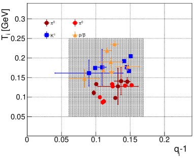
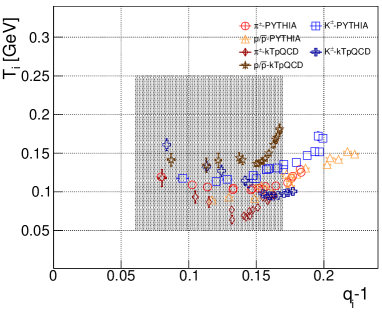
(a)	(b)

Figure 4: (a) The parameter space $T_{i}-q_{i}$ extracted from experimental $p_{T}$ spectra for hadron types $i\in$ $\pi^{\pm}$, $\pi^{0}$, $K^{\pm}$, $p$, and $\bar{p}$; (b) The PYTHIA and kTpQCD_20 calculated spectra fit results on the same hadron types added to the measurement fit points.

The calculated points are denoted by empty symbols for each identified hadron at several center-of-mass energies. Theoretical data fits partially overlap with the shaded area defined by the experimental fits, although several points are deviating.

PYTHIA8

We generated 10M events using PYTHIA8 artic:pythia6 ; artic:pythia8 Lund’s high-energy Monte Carlo event generator to simulate the identified hadron spectra. Points for (charge-averaged) pion, kaon and protons spread in the $q_{i}\in[1.08,1,23]$ range, wider than the experimental points. In contrast to that, the $T_{i}\in[80,150]$ MeV corresponding to the experimental values on the left panel. Deviating points of the PYTHIA8 results are those which lack sufficient statistics at the highest transverse momenta. Here, the tail of the distribution is indefinite, thus $q_{i}$ values fall outside of the experimental $q_{i}(\sqrt{s})\in[1.07,1.17]$ parameter space. One recognizes that pions deviate less, since they have the highest statistics among all, followed by kaons and protons. We note that the deviance of $q_{i}$ disappear as we exclude the low-statistic data at the highest momenta at each energy value, while the consistency with $T_{i}$ remains.

kTpQCD_v20

Hadron spectra calculated within the framework of perturbative QCD were also used utilizing kTpQCD_v20 artic:ktpqcd . These calculations deliver similar results for all hadron species, because of the similar (polynomial) fragmentation parametrizations. Concerning the correspondence between perturbative QCD results and experimental data fits, both $T_{i}$ and $q_{i}$ are running out of the experimental regime in a similar way. Deviation from the measurement-based data is most remarkable at low c.m. energies, where the $p_{T}$ range of the spectra is too short due to the limited phase-space. The domain of pQCD is $p_{T}>1.5$ GeV/$c$ and the maximal energy is typically $p_{T}<\sqrt{s}/2$. This limited range makes the fits more doubtful.

We also investigated the center-of-mass energy dependence of the fit parameters calculated theoretically from the the PYTHIA8 artic:pythia6 ; artic:pythia8 and kTpQCD_v20 artic:ktpqcd models. In Figure 5, we compare the experimentally observed $\sqrt{s}$-dependence from Figure 2 (solid lines) to these theoretical model results (data points). Figure 5a is for parameter $q_{i}$.

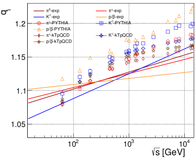
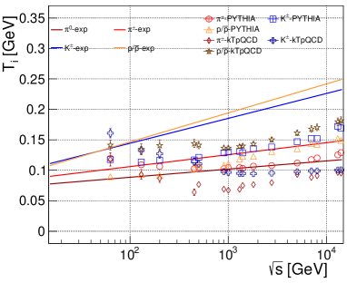
(a)	(b)

Figure 5: The fitted $q_{i}$ (a) and $T_{i}$ (b) as a function of $\sqrt{s}$ for hadron species, $i$ marked as points. Only the species of the particles are indicated by points. The solid color lines are fitted to the experimentally measured pion, kaon, and (anti)proton points.

Non-extensivity, $\boldsymbol{q_{i}}$:

According to the above observations, the perturbative QCD points are close to each other, due to the similar fragmentation function parametrization for the hardon species, mostly at the tail of the distributions at the highest energies and momenta—where experimental and theoretical data meet each other. With kTpQCD_v20 pions and kaons have similar slopes in $\log(\sqrt{s})$. PYTHIA8 results violate the inequality (31) and are larger: $q_{PYTHIA,i}>q_{EXP,i}$. However, the $\log(\sqrt{s})$ evolution has the same trend and similar slopes—except for protons.

Temperature-like, $\boldsymbol{T_{i}}$:

The kTpQCD_v20 points for each hadron species are close to each other and meet the temperature values only at the highest-energy regime. In this case the formula (32) represents a trend opposite to the perturbative QCD calculations. Theoretical fit parameters deviate here appreciably. We count this for the non-applicability of the pQCD at the low-momentum regime, $p_{T}<1.5$ GeV/$c$, where the spectra are more thermal-like. On the other hand, PYTHIA8 works well for both the soft and hard regimes for the light hadrons. The $\sqrt{s}$ evolution follows the experimentally observed trend, only a small offset is present for kaons and protons.

We conclude that these model calculations proved their validity in several ways artic:predict1 ; artic:predict2 . Nevertheless, these pictures are not fully consistent with the fit parameters obtained from the data. In other words, comparison of theoretical models should be made with care within their region of validity.

5 Comparison with the Improved Quark-Coalescence Model

As we have explained in Section 3.4, the quark-coalescence model was developed for heavy-ion collisions originally, but it was improved by the previously introduced Tsallis distribution. In the followings we endeavor to extend this idea also for smaller systems, such as proton-proton collisions.

5.1 Connecting Non-Extensivity with the Quark-Coalescence Model

According to the coalescence picture, the observed of $(q_{meson}-1)/(q_{baryon}-1)$ should be $3/2$ artic:quarkscaling .

In Figure 6 we plot the ratio $\chi_{ij}=(q_{i}-1)/(q_{j}-1)$ as a function of the center-of-mass energy, $\sqrt{s}$. Figure 6a presents the ratios of experimental data points compared to the fit curve ratios of $\pi/p$, $K/p$ and $K/p$ listed in Table 1. A monotonic, increasing trend of the ratios is clearly seen at the lower energies and saturation can be expected in the most energetic reactions. There are two important observations that is worth note:

1. the $(q_{meson}-1)/(q_{baryon}-1)$ fit curves lie below the dashed line with the value of $3/2$ within the $\sqrt{s}\in[62.4~{}\textrm{GeV},10~{}\textrm{TeV}]$ c.m. energy range;

2. the $\chi_{K\pi}$ kaon-pion ratio shoots over the expected value, 1, a bit.

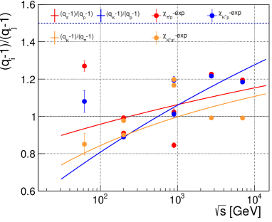
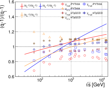
(a)	(b)

Figure 6: (a) Ratio of $(q_{meson}-1)/(q_{baryon}-1)$ plotted in the function of $\sqrt{s}$ as data points and fit lines. (b) The PYTHIA and kTpQCD_20 calculated spectra fit results on the same hadron types added to the measurement fit lines.

On Figure 6b we plotted the theoretically calculated points along with the experimentally fitted solid lines. It is not surprising, that theoretical curves present quite flat functions for all combination of the ratios, since both the PYTHIA8’s Lund fragmentation and the fragmentation function parametrizations in the kTpQCD_v20 are based on the constituent quark model and the infinite momentum frame is assumed as well. Thus, there is no room for the evolution apart from a constant hadron-mass effect. This can result only in a shift of the $q_{i}$ values as we have seen on the left panel of Figure 5. Deviation from the constancy appears only at the lowest energies, but as we have seen earlier in Section 4.1, at low energies both PYTHIA8 and kTpQCD_v20 have limited phase space. The average values of the ratios $\chi_{ij}=(q_{i}-1)/(q_{j}-1)$ are summarized in Table 3 for $i,j\in\{\pi,K,p\}$.

Table 3: The average values of the hadron spectra parameter ratios, $\chi_{ij}=(q_{i}-1)/(q_{j}-1)$, obtained from theoretical models PYTHIA8 and kTpQCD_v20.

Hadron Ratio	PYTHIA8	kTpQCD_v20	Colaescence
$\chi_{K\pi}$	$1.09\pm 0.01$	$1.10\pm 0.01$	$1.0$
$\chi_{Kp}$	$0.95\pm 0.01$	$1.06\pm 0.01$	$1.5$
$\chi_{\pi p}$	$0.87\pm 0.01$	$0.94\pm 0.01$	$1.5$

The kTpQCD_v20- and PYTHIA8-calculated $(q_{i}-1)/(q_{j}-1)$ points have the same order:

$$\chi_{K\pi}>\chi_{Kp}>\chi_{\pi p}\ \ \ .$$ (33)

For $\chi_{K\pi}$ both models give the same value, $10\%$ larger than the improved coalescence expectation of 1. For $\chi_{meson,baryon}$ kTpQCD_v20 has slightly higher values than PYTHIA8, but both are far below the expected value 3/2. Comparing the experimental fit curves and the theoretically calculated points, both theory meets the experimental values of $\chi_{K\pi}$. However, for $\chi_{meson,baryon}$ the kTpQCD_v20 model agrees with the experimental values only at the highest $\sqrt{s}$ c.m. energies.

In summary the improved quark-coalescence model prediction might be reached only beyond the LHC energies, now they seem to support the smaller values. Allegedly, constituent-quark scaling is a high-$\sqrt{s}$ property. Experimental data support the trends, the very hadronizaton model needs further investigation.

5.2 Investigating the $T_{Slope}$ in the Quark-Coalescence Model

In the quark-coalescence model, $T_{hadron}=T_{parton}=T$, thus $T_{meson}=T_{baryon}$ is also assumed, c.f. Section 3.4. Using the Tsallis distribution we consider the logarithmic slope of $E_{i}$ spectra:

$$T_{slope}=\left[-\frac{{\textrm{d}}}{{\textrm{d}}E_{i}}\ln P_{i}\right]^{-1}=T+(q-1)E_{i}\ \ \ .$$ (34)

This may explain the mass ordering found in Equation (32). A possible way to read off this effect would be to determine the slope of $(m_{T,i}-m_{i})$ spectra. Estimating $E_{i}$ by $\sqrt{s}-m_{i}$ one obtains results as seen in Figure 7.

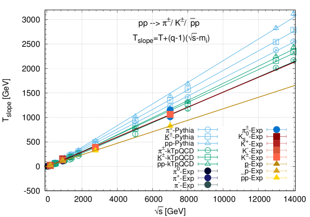
Figure 7: The $T_{slope}(\sqrt{s})$ curves defined by Equation (34), fitted on the theoretical PYTHIA8 and kTpQCD_v20 data (empty points) and on the experimental values (solid points), for all investigated hadron species.

6 Summary and Discussion

In this study we analyzed identified hadron spectra measured in proton-proton collisions from RHIC to LHC energies in the range $62.4$ GeV $\leq\sqrt{s}\leq 7$ TeV. We showed that the Tsallis–Pareto distributions originated from non-extensive thermodynamics describe the spectra very well in wide $m_{T}$ regions, typically at $p_{T}\lesssim$ 10–20 GeV/$c$ using the distribution in the form of Equation (20).

We provided a comprehensive and detailed analysis of the state-of-the-art experimental data which will be used also to make predictions about the forthcoming 13 TeV and 14 TeV spectra. The $\sim\log(\sqrt{s})$-like evolution of the parameters $q_{i}$ and $T_{i}$ were tested on the identified hadron spectra data measured for charge averaged $\pi^{\pm}$, $\pi^{0}$, $K^{\pm}$, $p$, and $\bar{p}$. We observed that both the non-extensivity parameter $q_{i}$ and temperature-like $T_{i}$ parameters agree with the suggested QCD-inspired evolution pattern. However, the temperature has almost a constant value within the investigated center-of-mass energy regime. We found a mass-ordered hierarchy in the evolution parameters of the experimental fits, i.e., lighter hadron spectra have the more non-extensive $q_{i}>1$ and heavier hadron spectra fit with larger $T_{i}$ values. However, we note that the deduced $T_{i}$ values might be sensitive not just the hadron mass but also on the chosen distribution function. This might result different values extracted from similar data, e.g., in reference artic:cleymansTS .

We compared the experimental data fit results with theoretical predictions. The c.m. energy evolution of the fit parameters were calculated by PYTHIA8 artic:pythia6 ; artic:pythia8 and kTpQCD_v20 artic:ktpqcd . We found theoretical fit parameters to be more compact in the $(T,q)$ space than the experimental ones: $T_{i}\in[80,240]$ MeV, while non-extensivity is wider than the measurement-based $q_{i}\in[1.08,1,23]$ region. The most deviating points arise from limitations of the theoretical models, i.e., where statistics is low or the phase-space is limited. Energy evolution in the theoretical models were investigated as well. In agreement with our expectations we conclude that

1. for the $\sqrt{s}$ evolution, kTpQCD_v20 agrees more with the power-law related non-extensivity parameter $q_{i}$;

2. PYTHIA8 results correspond well with the measured $T_{i}(\sqrt{s})$ evolution.

The study of these models reflected the lack of the proper handling of the hadron-mass, since all assumptions fail for more massive hadron species.

At the highest energies and momenta, in the infinite momentum frame, constituent quark number scaling is assumed to get stronger. To test this idea in the framework of the non-extensive approach, we applied and investigated an improved quark-coalescence model, inserting Tsallis-like energy distribution kernels where constituent quark scaling appears explicitly. Experimental data present a slight monotonic-increase with c.m. energy, but the saturation ridge of the ratio $(q_{meson}-1)/(q_{baryon}-1)$ is lower than predicted by the coalescence-theory (3/2) while the reference ratio $(q_{meson}-1)/(q_{meson^{\prime}}-1)$ is only slightly apart from the expected value $1$. The fit parameters calculated by PYTHIA8 and kTpQCD_v20 models both have almost no $\sqrt{s}$ evolution, but only the ratio values for light mesons are in agreement with the experimental data especially at the highest LHC energies.

In summary, our detailed analysis aimed to investigate how we can provide physical meaning for experimentally-fitted parameters, based on well-known theoretical models and phenomena. Our results motivate us to improve the model of hadronization in high-energy collisions, using spectra with exponential shape at low-$p_{T}$, keeps the power-law tail at thigh $p_{T}$, and takes care of the meson/baryon spectra ratios and/or the experimentally observed $(q_{meson}-1)/(q_{barion}-1)$.

Appendix A

In Table A1 we show the parameters fitted to all used datasets artic:62gevphenix ; artic:62gevphenix2 ; artic:200gevphenix ; artic:200gevstar ; artic:500gevphenix ; artic:09tevalice ; artic:097tevalice ; artic:276tevalice ; artic:276tevpi0alice ; artic:7tevalice ; artic:7tevalice2 . The parameters $q_{i}$, $T_{i}$ and $A_{i}$ from Equation (20). and the $\chi^{2}/$ndf values of the given fit are listed for each identified hadron and for each $\sqrt{s}$ center-of-mass energy value.

Table A1: The fitted $q$, $T$ and $A$ parameters and the $\chi^{2}$/ndf value of the fit for identified hadrons $\pi^{0}$, $\pi^{\pm}$, $K^{\pm}$ and $p\bar{p}$. The values are grouped according to the hadrons such that the change in respect to the center-of-mass energy can be compared easily.

$\sqrt{s}$ (GeV)	Hadron	$q$	$T$ (GeV)	$A$	$\chi^{2}/$ndf	Experiment
62	$\pi^{0}$	1.073 $\pm$ 0.011	0.139 $\pm$ 0.027	121.252 $\pm$ 100.460	7.857/11	PHENIX artic:62gevphenix2
200	$\pi^{0}$	1.101 $\pm$ 0.002	0.133 $\pm$ 0.003	149.459 $\pm$ 15.459	6.450/14	PHENIX artic:62gevphenix
500	$\pi^{0}$	1.128 $\pm$ 0.000	0.098 $\pm$ 0.000	746.070 $\pm$ 0.527	3656.733/25	PHENIX artic:500gevphenix
900	$\pi^{0}$	1.132 $\pm$ 0.029	0.128 $\pm$ 0.046	302183.366 $\pm$ 321455.697	0.462/10	ALICE artic:097tevalice
2760	$\pi^{0}$	1.137 $\pm$ 0.009	0.141 $\pm$ 0.035	4.937 $\pm$ 5.116	0.237/15	ALICE artic:276tevpi0alice
7000	$\pi^{0}$	1.146 $\pm$ 0.004	0.140 $\pm$ 0.010	498950.603 $\pm$ 133429.129	1.143/30	ALICE artic:097tevalice
62	$\pi^{\pm}$	1.106 $\pm$ 0.000	0.100 $\pm$ 0.000	245.248 $\pm$ 0.000	4.276/23	PHENIX artic:62gevphenix
200	$\pi^{+}$	1.112 $\pm$ 0.001	0.089 $\pm$ 0.005	39.389 $\pm$ 14.396	58.248/11	STAR artic:200gevstar
200	$\pi^{-}$	1.110 $\pm$ 0.001	0.087 $\pm$ 0.005	48.554 $\pm$ 18.250	75.053/11	STAR artic:200gevstar
900	$\pi^{+}$	1.124 $\pm$ 0.000	0.133 $\pm$ 0.000	4.496 $\pm$ 0.000	4.413/12	ALICE artic:09tevalice
900	$\pi^{-}$	1.124 $\pm$ 0.002	0.127 $\pm$ 0.001	5.240 $\pm$ 0.082	10.816/30	ALICE artic:09tevalice
2760	$\pi^{\pm}$	1.143 $\pm$ 0.000	0.129 $\pm$ 0.000	12.546 $\pm$ 0.000	3.929/60	ALICE artic:276tevalice
7000	$\pi^{\pm}$	1.152 $\pm$ 0.000	0.131 $\pm$ 0.000	14.544 $\pm$ 0.000	5.750/55	ALICE artic:7tevalice ; artic:7tevalice2
62	$K^{\pm}$	1.090 $\pm$ 0.050	0.161 $\pm$ 0.033	3.142 $\pm$ 1.155	0.192/13	PHENIX artic:62gevphenix
200	$K^{+}$	1.109 $\pm$ 0.001	0.122 $\pm$ 0.002	0.902 $\pm$ 0.187	31.664/12	STAR artic:200gevstar
200	$K^{-}$	1.083 $\pm$ 0.005	0.199 $\pm$ 0.116	0.091 $\pm$ 0.058	17.189/11	STAR artic:200gevstar
900	$K^{+}$	1.148 $\pm$ 0.000	0.167 $\pm$ 0.000	0.203 $\pm$ 0.000	6.932/24	ALICE artic:09tevalice
900	$K^{-}$	1.145 $\pm$ 0.000	0.176 $\pm$ 0.000	0.186 $\pm$ 0.000	19.465/24	ALICE artic:09tevalice
2760	$K^{\pm}$	1.141 $\pm$ 0.002	0.192 $\pm$ 0.004	0.434 $\pm$ 0.022	2.793/55	ALICE artic:276tevalice
7000	$K^{\pm}$	1.151 $\pm$ 0.000	0.205 $\pm$ 0.000	0.500 $\pm$ 0.000	3.756/48	ALICE artic:7tevalice ; artic:7tevalice2
62	$p/\bar{p}$	1.083 $\pm$ 0.022	0.147 $\pm$ 0.023	1.240 $\pm$ 0.440	4.722/24	PHENIX artic:62gevphenix
200	$p$	1.118 $\pm$ 0.001	0.070 $\pm$ 0.001	10.205 $\pm$ 13.089	15.983/11	STAR artic:200gevstar
200	$\bar{p}$	1.109 $\pm$ 0.001	0.074 $\pm$ 0.003	9.945 $\pm$ 2.227	26.393/11	STAR artic:200gevstar
900	$p$	1.146 $\pm$ 0.017	0.178 $\pm$ 0.009	0.053 $\pm$ 0.003	13.758/21	ALICE artic:09tevalice
900	$\bar{p}$	1.122 $\pm$ 0.017	0.190 $\pm$ 0.010	0.049 $\pm$ 0.002	13.337/21	ALICE artic:09tevalice
2760	$p/\bar{p}$	1.116 $\pm$ 0.006	0.219 $\pm$ 0.007	0.110 $\pm$ 0.005	2.232/45	ALICE artic:276tevalice
7000	$p/\bar{p}$	1.127 $\pm$ 0.006	0.236 $\pm$ 0.007	0.117 $\pm$ 0.005	2.556/46	ALICE artic:7tevalice ; artic:7tevalice2

Appendix B

In Table A2 the used datasets, their kinematical properties and the corresponding references are listed. As we already mentioned in Section 4. that the spectra were measured in wide range of kinematical variables, although these values varies in different experiments.

$\sqrt{s}$ (TeV)	Rapidity	Particle	$p_{T}$ Range [GeV/$c$]	Experiment
0.062	$|\eta|<0.35$	$\pi^{0}$	$0.5\leq p_{T}\leq 7$	PHENIX artic:62gevphenix2
		$\pi^{\pm}$	$0.3\leq p_{T}\leq 3$	PHENIX artic:62gevphenix
		$K^{\pm}$	$0.5\leq p_{T}\leq 2$
		$p/\bar{p}$	$1\leq p_{T}\leq 4$
0.2	$|\eta|<0.35$	$\pi^{0}$	$1\leq p_{T}\leq 15$	PHENIX artic:200gevphenix
	$|y|<0.5$	$\pi^{\pm}$	$3\leq p_{T}\leq 15$	STAR artic:200gevstar
		$K^{\pm}$	$3\leq p_{T}\leq 15$
		$p/\bar{p}$	$3\leq p_{T}\leq 15$
0.5	$|\eta|<0.35$	$\pi^{0}$	$1\leq p_{T}\leq 30$	PHENIX artic:500gevphenix
0.9	$|y|<0.5$	$\pi^{0}$	$0.4\leq p_{T}\leq 7$	ALICE artic:097tevalice
		$\pi^{\pm}$	$0.1\leq p_{T}\leq 2.5$	ALICE artic:09tevalice
		$K^{\pm}$	$0.2\leq p_{T}\leq 2.5$
		$p/\bar{p}$	$0.3\leq p_{T}\leq 2.5$
2.76	$|\eta|<0.8$	$\pi^{0}$	$0.6\leq p_{T}\leq 20$	ALICE artic:276tevpi0alice
		$\pi^{\pm}$	$0.1\leq p_{T}\leq 20$	ALICE artic:276tevalice
		$K^{\pm}$	$0.1\leq p_{T}\leq 20$
		$p/\bar{p}$	$0.3\leq p_{T}\leq 15$
7	$|y|<0.5$	$\pi^{0}$	$0.3\leq p_{T}\leq 25$	ALICE artic:097tevalice
		$\pi^{\pm}$	$0.1\leq p_{T}\leq 20$	ALICE artic:7tevalice ; artic:7tevalice2
		$K^{\pm}$	$0.2\leq p_{T}\leq 20$
		$p/\bar{p}$	$0.3\leq p_{T}\leq 20$

Table A2: The used datasets and their kinematic properties (including the center-of-mass energy, the rapidity window and the transverse momentum range) used for fitting, with the reference for the corresponding article.

References

- (1) Gell-Mann, M.; Tsallis, C. Possible generalization of Boltzmann-Gibbs statistics. In Nonextensive Entropy-Interdisciplinary Applications; Oxford University Press: Oxford, UK, 2004
- (2) Tsallis, C. Introduction to Nonextensive Statistical Mechanics; Springer: New York, NY, USA, 2009
- (3) Sébenne, C.; Morrison, G. Nonextensive statistical mechanics: New trends, new perspectives. Europhys. News Spec. Issue 2005, 36, doi:10.1051/epn:2005601.
- (4) Tarmissi, K.; Hamza, A.B. Information-theoretic hashing of 3D objects using graph theory. Expert Syst. Appl. 2009, 36, 9409–9414.
- (5) Khader, M.; Hamza, A.B. An information-theoretic method for multimodality medical image registration. Expert Syst. Appl. 2012, 39, 5548–5556.
- (6) Furuichi, S.; Mitroi-Symeonidis, F.C.; Symeonidis, E. On Some Properties of Tsallis Hypoentropies and Hypodivergences. Entropy 2014, 16, 5377–5399.
- (7) List of Application of the Tsallis Distribution. Available online: \changeurlcolorblackhttp://tsallis.cat.cbpf.br/biblio.htm\changeurlcolorblue (accessed on 27 January 2017).
- (8) Jaffe, A.; Witten, E. Quantum Yang-Mills theory, Official Problem Description. Available online: \changeurlcolorblackhttp://www.claymath.org/sites/default/files/yangmills.pdf\changeurlcolorblue (accessed on 27 January 2017).
- (9) Ürmössy, K.; Barnaföldi, G.G.; Biró, T.S. Generalised Tsallis Statistics in Electron-Positron Collisions. Phys. Lett. B 2011, 701, 111–116.
- (10) Ürmössy, K.; Biró, T.S. Cooper-Frye Formula and Non-extensive Coalescence at RHIC Energy. Phys. Lett. B 2010, 689, 14–17.
- (11) Ürmössy, K.; Biró, T.S.; Barnaföldi, G.G.; Xu, Z. Disentangling Soft and Hard Hadron Yields in PbPb Collisions at ATeV. arXiv 2014, arXiv:1405.3963.
- (12) Ürmössy, K.; Biró, T.S.; Barnaföldi, G.G.; Xu, Z. v2 of charged hadrons in a ‘soft + hard’ model for PbPb collisions at ATeV. arXiv 2014, arXiv:1501.05959.
- (13) Barnaföldi, G.G.; Ürmössy, K.; Bíró, G. A ’soft + hard’ model for Pion, Kaon, and Proton Spectra and v2 measured in PbPb Collisions at = 2.76 ATeV. J. Phys. Conf. Ser. 2015, 612, 012048.
- (14) Biró, T.S.; Purcsel, G.; Ürmössy, K. Non-Extensive Approach to Quark Matter. Eur. Phys. J. 2009, A40, 325–340.
- (15) Cleymans, J.; Lykasov, G.I.; Parvan, A.S.; Sorin, A.S.; Teryaev, O.V.; Worku, D. Systematic properties of the Tsallis Distribution: Energy Dependence of Parameters in High-Energy p-p Collisions. Phys. Lett. B 2013, 723, 351–354.
- (16) Cleymans, J.; Azmi, M.D. Large Transverse Momenta and Tsallis Thermodynamics. J. Phys. Conf. Ser. 2016, 668, 012050.
- (17) Wong, C.; Wilk, G.; Cirto, L.J.L.; Tsallis, C. From QCD-based hard-scattering to nonextensive statistical mechanical descriptions of transverse momentum spectra in high-energy and collisions. Phys. Rev. D 2015, 91, 114027.
- (18) Wong, C.; Wilk, G.; Cirto, L.J.L.; Tsallis, C. Possible Implication of a Single Nonextensive pTpT Distribution for Hadron Production in High-Energy pp Collisions. EPJ Web Conf. 2015, 90, 04002.
- (19) Wilk, G.; Wlodarczyk, Z. Multiplicity fluctuations and temperature fluctuations in high-energy nuclear collisions. Phys. Rev. C 2009, 79, 054903.
- (20) Wilk, G.; Wlodarczyk, Z. On Possible Origins of Power-law distributions. AIP Conf. Proc. 2013, 1558, 893.
- (21) Tsallis, C. Possible generalization of Boltzmann-Gibbs statistics. J. Stat. Phys. 1988, 52, 497–487.
- (22) Wilk, G.; Włodarczyk, Z. Tsallis Distribution Decorated with Log-Periodic Oscillation. Entropy 2015, 17, 384–400.
- (23) Wilk, G.; Włodarczyk, Z. Quasi-power Law Ensembles. Acta Phys. Pol. B 2015, 46, 1103–1122.
- (24) Wilk, G.; Włodarczyk, Z. Quasi-power laws in multiparticle production processes. Chaos Solitons Fract. 2015, 81, 487–496.
- (25) Zheng, H.; Lilin, Z. Can Tsallis Distribution Fit All the Particle Spectra Produced at RHIC and LHC? Adv. High Energy Phys. 2015, 2015, 180491.
- (26) Zheng, H.; Lilin, Z.; Bonasera, A. Systematic analysis of hadron spectra in p + p collisions using Tsallis distributions. Phys. Rev. D 2015, 92, 074009.
- (27) Cleymans, J. On the Use of the Tsallis Distribution at LHC Energies. arXiv 2016, arXiv:1609.02289.
- (28) Cleymans, J. The Tsallis Distribution for p p collisions at the LHC. J. Phys. Conf. Ser. 2013, 455, 012049.
- (29) Bjorken, J.D. Asymptotic Sum Rules at Infinite Momentum. Phys. Rev. 1969, 179, 1547.
- (30) PHENIX Collaboration. Measurement of and in p + p, d+Au and Cu+Cu collisions at = 200 GeV. Phys. Rev. C 2014, 90, 054905.
- (31) STAR Collaboration. Strange particle production in p + p collisions at 200 GeV. Phys. Rev. C 2007, 75, 064901.
- (32) CMS Collaboration. Study of the inclusive production of charged pions, kaons, and protons in pp collisions at = 0.9, 2.76, and 7 TeV. Eur. Phys. J. C 2012, 72, 2164.
- (33) ATLAS Collaboration. Charged-particle multiplicities in pp interactions measured with the ATLAS detector at the LHC. New J. Phys. 2011, 13, 053033.
- (34) PHENIX Collaboration. Identified charged hadron production in p + p collisions at and GeV. Phys. Rev. C 2011, 83, 064903.
- (35) ALICE Collaboration. Neutral pion and meson production in proton-proton collisions at TeV and TeV. Phys. Lett. B 2012, 717, 162–172.
- (36) Hagedorn, R. Multiplicities, distributions and the expected hadron quark-gluon phase transition. Nuovo Cimento 1983, 6, 1–50.
- (37) UA1 Collaboration. Transverse momentum spectra for charged particles at the CERN proton-antiproton collider. Phys. Lett. B 1982, 118, 167–172.
- (38) UA1 Collaboration. Production of Low Transverse Energy Clusters in anti-p p Collisions at -TeV to 0.9-TeV and their Interpretation in Terms of QCD Jets. Nucl. Phys. B 1988, 309, 405–425.
- (39) Michael, C.; Vanryckeghem, L. Consequences of momentum conservation for particle production at large transverse momentum. J. Phys. G Nucl. Phys. 1977, 3, L151.
- (40) Michael, C. Large transverse momentum and large mass production in hadronic interactions. Prog. Part. Nucl. Phys. 1979, 2, 1–39.
- (41) Biró, T.S.; Ván, P.; Barnaföldi, G.G.; Ürmössy, K. Statistical Power Law due to Reservoir Fluctuations and the Universal Thermostat Independence Principle. Entropy 2014, 16, 6497–6514.
- (42) Biró, T.S.; Ván, P.; Barnaföldi, G.G.; Ván, P. New Entropy Formula with Fluctuating Reservoir. Physica 2015, 417, 215–220.
- (43) Cleymans, J.; Worku, D. The Tsallis distribution in proton–proton collisions at = 0.9 TeV at the LHC. J. Phys. G 2012, 39, 025006.
- (44) Santos, A.P.; Pereira, F.I.M.; Silva, R.; Alcaniz, J.S. Consistent nonadditive approach and nuclear equation of state. J. Phys. G 2014, 41, 055105.
- (45) Deppman, A. Properties of hadronic systems according to the nonextensive self-consistent thermodynamics. J. Phys. G 2014, 41, 055108.
- (46) Megías, E.; Menezes, D.P.; Deppman, A. Non extensive thermodynamics for hadronic matter with finite chemical potentials. Physica A 2015, 421, 15–24.
- (47) Biró, T.S. Is there a Temperature? Conceptual Challenges at High Energy, Acceleration and Complexity; Springer: Berlin/Heidelberg, Germany, 2011.
- (48) Biró, T.S.; Ván, P.; Barnaföldi, G.G.; Ván, P. Quark-gluon plasma connected to finite heat bath. Eur. Phys. J. 2013, A49, 110.
- (49) Altarelli, G.; Parisi, G. Asymptotic Freedom in Parton Language. Nucl.Phys. B 1977, 126, 298–318.
- (50) Dokshitser, Y. L. Calculation of structure functions of deep-inelastic scattering and e + e-annihilation by perturbation theory in quantum chromodynamics. Sov. Phys. JETP 1977, 46, 641–653.
- (51) Gribov, V.N.; Lipatov, L.N. Deep inelastic e p scattering in perturbation theory. Sov. J. Nucl. Phys. 1972, 15, 438–450.
- (52) Patrignani, C.; Agashe, K.; Aielli, G.; Amsler, C.; Antonelli, M.; Asner, D.M.; Baer, H.; Banerjee, S.; Barnett, R.M.; Basaglia, T.; et al. Particle Data Group. Chin. Phys. C 2016, 40, 100001.
- (53) Altarelli, G.; Ellis, R.K.; Martinelli, G. Leptoproduction and Drell-Yan processes beyond the leading approximation in chromodynamics. Nucl. Phys. B 1978, 143, 521–545.
- (54) Barnaföldi, G.G.; Biró, T. S.; Ürmössy, K.; Kalmár, G. Tsallis-Pareto-like distributions in hadron-hadron collisions. Gribov-80 Memorial Volume: Quantum Chromodynamics and Beyond. J. Phys. Conf. Ser. 2010, 270, 012008.
- (55) Biró, T.S.; Ürmössy, K. ALCOR. Eur. Phys. J. Spec. Top. 2008, 155, 1–12.
- (56) Biró, T.S.; Lévai P.; Zimányi, J. ALCOR: A dynamical model for hadronization. Phys. Lett. B. 1995, 347, 6–12.
- (57) PHENIX Collaboration. Inclusive cross section and double helicity asymmetry for production in p + p collisions at GeV. Phys. Rev. D 2009, 79, 012003.
- (58) PHENIX Collaboration. Mid-Rapidity Neutral Pion Production in Proton-Proto Collisions at GeV. Phys. Rev. Lett. 2003, 91, 241803.
- (59) STAR Collaboration. Identified hadron compositions in p + p and Au+Au collisions at high transverse momenta at GeV. Phys. Rev. Lett. 2012, 108, 072302.
- (60) PHENIX Collaboration. Inclusive cross section and double-helicity asymmetry for production at midrapidity in p + p collisions at GeV. Phys. Rev. D 2016, 93, 011501.
- (61) ALICE Collaboration. Production of pions, kaons and protons in pp collisions at GeV with ALICE at the LHC. Eur. Phys. J. C 2010, 71, 1655.
- (62) ALICE Collaboration. Production of charged pions, kaons and protons at large transverse momenta in pp and Pb-Pb collisions at TeV. Phys. Lett. B 2014, 736, 196–207.
- (63) ALICE Collaboration. Neutral pion production at midrapidity in pp and Pb-Pb collisions at TeV. Eur. Phys. J. C 2014, 74, 3108.
- (64) ALICE Collaboration. Measurement of pion, kaon and proton production in proton-proton collisions at TeV. Eur. Phys. J. C 2015, 75, 226.
- (65) ALICE Collaboration. Multiplicity dependence of charged pion, kaon, and (anti)proton production at large transverse momentum in p-Pb collisions at TeV. Phys. Lett. B 2016, 760, 720.
- (66) Ürmössy, K. Multiplicity Dependence of Hadron Spectra in Proton-proton Collisions at LHC Energies and Super-statistics. arXiv 2012, arXiv:1212.0260.
- (67) Borsanyi, S.; Fodor, Z.; Guenther, J.; Kampert, K.-H.; Katz, S.D.; Kawanai, T.; Kovacs, T.G.; Mages, S.W.; Pasztor, A.; Pittler, F.; et al. Calculation of the axion mass based on high-temperature lattice quantum chromodynamics. Nature 2016, 539, 69–71.
- (68) Sjostrand, T.; Mrenna, S.; Skands, P. PYTHIA 6.4 Physics and Manual. J. High Energy Phys. 2006, 5, 026.
- (69) Sjostrand, T.; Mrenna, S.; Skands, P. An Introduction to PYTHIA 8.2. Comput. Phys. Commun. 2015, 191, 159–177.
- (70) Zang, Y.; Fai, G.; Papp, G.; Barnaföldi, G.G.; Lévai, P. High- pion and kaon production in relativistic nuclear collisions. Phys. Rev. C 2002, 65, 034903.
- (71) Albacete, J.L.; Arleo, F.; Barnafoldi, G.G.; Barrette, J.; Deng, W.-T.; Dumitru, A.; Eskola, K.J.; Ferreiro, E.G.; Fleuret, F.; Fujii, H.; et al. Predictions for p + Pb Collisions at = 5 TeV: Comparison with Data. Int. J. Mod. Phys. E 2016, 25, 1630005.
- (72) Albacete, J.L.; Arleo, F.; Barnafoldi, G.G.; Barrette, J.; Deng, W.-T.; Dumitru, A.; Eskola, K.J.; Ferreiro, E.G.; Fleuret, F.; Fujii, H.; et al. Predictions for p + Pb Collisions at = 5 TeV. Int. J. Mod. Phys. E 2013, 22, 1330007.
- (73) Biró, T.S.; Ürmössy, K. Pions and kaons from stringy quark matter. J. Phys. G 2009, 36, 064044.