The DTM-signature for a geometric comparison of metric-measure spaces from samples

Abstract

In this paper, we introduce the notion of DTM-signature, a measure on $\mathbbm{R}_{+}$ that can be associated to any metric-measure space. This signature is based on the distance to a measure (DTM) introduced by Chazal, Cohen-Steiner and Mérigot. It leads to a pseudo-metric between metric-measure spaces, upper-bounded by the Gromov-Wasserstein distance. Under some geometric assumptions, we derive lower bounds for this pseudo-metric.

Given two $N$-samples, we also build an asymptotic statistical test based on the DTM-signature, to reject the hypothesis of equality of the two underlying metric-measure spaces, up to a measure-preserving isometry. We give strong theoretical justifications for this test and propose an algorithm for its implementation.

1 Introduction

Among the variety of data available, from astrophysics to biology, including social networks and so on, many come as sets of points from a metric space. A natural question, given two sets of such data is to decide whether they are similar, that is whether they come from the same distribution, whether their shape are close, or not. This comparison may be compromised when the data are not embedded into the same space, or if the two systems of coordinates in which the data are represented are different. To overcome this issue, a natural idea is to forget about this embedding and only consider the set of points together with the distances between pairs. A natural framework to compare data is then to assume that they come from a measure on a metric space and to consider two such metric-measure spaces as being the same when they are equal up to some isomorphism, as defined below.

Definition 1 (mm-space).

A metric-measure space (mm-space) is a triple $(\mathcal{X},\delta,\mu)$, with $\mathcal{X}$ a set, $\delta$ a metric on $\mathcal{X}$ and $\mu$ a probability measure on $\mathcal{X}$ equipped with its Borel $\sigma$-algebra.

Definition 2 (Isomorphism between mm-spaces).

Two mm-spaces $(\mathcal{X},\delta,\mu)$ and $(\mathcal{Y},\gamma,\nu)$ are said to be isomorphic if their exist Borel sets $\mathcal{X}_{0}\subset\mathcal{X}$ and $\mathcal{Y}_{0}\subset\mathcal{Y}$ such that $\mu(\mathcal{X}\backslash\mathcal{X}_{0})=0$ and $\nu(\mathcal{Y}\backslash\mathcal{Y}_{0})=0$, and some one-to-one and onto isometry $\phi:\mathcal{X}_{0}\rightarrow\mathcal{Y}_{0}$ preserving measures, that is satisfying $\nu(\phi(A\cap\mathcal{X}_{0}))=\mu(A\cap\mathcal{X}_{0})$ for any Borel set $A$ of $\mathcal{X}$. Such a map $\phi$ is called an isomorphism between the mm-spaces $(\mathcal{X},\delta,\mu)$ and $(\mathcal{Y},\gamma,\nu)$.

In this paper, we first address the question of the comparison of general mm-spaces, up to an isomorphism. In other terms, we aim at designing a metric or at least a pseudo-metric on the quotient space of mm-spaces by the relation of isomorphism. A suitable pseudo-distance should be stable under some perturbations, under sampling, discriminative and easy to implement when dealing with discrete spaces.

A first characterisation of mm-spaces is given in [19]. In its Theorem $3\frac{1}{2}.5$, Gromov proves that any mm-space can be recovered, up to an isomorphism, from the knowledge, for all size $N$, of the distribution of the $N\times N$-matrix of distances associated to a $N$-sample. More recently, in [23], Mémoli proposes metrics on the quotient space of mm-spaces by the relation of isomorphism, the Gromov–Wasserstein distances.

Definition 3 (Gromov–Wasserstein distance).

The Gromov–Wasserstein distance between two mm-spaces $(\mathcal{X},\delta,\mu)$ and $(\mathcal{Y},\gamma,\nu)$ with parameter $p\in[1,\infty)$ denoted $GW_{p}(\mathcal{X},\mathcal{Y})$ is defined by the expression:

$$\inf_{\pi\in\Pi(\mu,\nu)}\frac{1}{2}\left(\int_{\mathcal{X}\times\mathcal{Y}}\int_{\mathcal{X}\times\mathcal{Y}}\left(\Gamma_{\mathcal{X},\mathcal{Y}}\left(x,y,x^{\prime},y^{\prime}\right)\right)^{p}\pi(\rm d\it x\times\rm d\it y)\pi(\rm d\it x^{\prime}\times\rm d\it y^{\prime})\right)^{\frac{1}{p}},$$

with $\Gamma_{\mathcal{X},\mathcal{Y}}(x,y,x^{\prime},y^{\prime})=\left|\delta(x,x^{\prime})-\gamma(y,y^{\prime})\right|$. Here $\Pi(\mu,\nu)$ stands for the set of transport plans between $\mu$ and $\nu$, that is the set of Borel probability measures $\pi$ on $\mathcal{X}\times\mathcal{Y}$ satisfying $\pi(A\times\mathcal{Y})=\mu(A)$ and $\pi(\mathcal{X}\times B)=\nu(B)$ for all Borel sets $A$ in $\mathcal{X}$ and $B$ in $\mathcal{Y}$.

Unfortunately, even when dealing with discrete mm-spaces, the computation of these Gromov–Wasserstein distances is extremely costly. An alternative is to build a signature from each mm-space, that is an object invariant under isomorphism. The mm-spaces are then compared through their signatures. In [23], Mémoli gives an overview of such signatures, as for instance shape distribution, eccentricity or what he calls local distribution of distances.

In this paper, we introduce a new signature that is a probability measure on $\mathbbm{R}$, and we propose to compare such signatures using Wasserstein distances [26].

Definition 4 (Wasserstein distance).

The Wasserstein distance of parameter $p\in[1,\infty)$ between two Borel probability measures $\mu$ and $\nu$ over the same metric space $(\mathcal{X},\delta)$ is defined as:

$$W_{p}(\mu,\nu)=\inf_{\pi\in\Pi(\mu,\nu)}\left(\int_{\mathbbm{R}^{2}}\delta^{p}(x,y)\rm d\it\pi(x,y)\right)^{\frac{1}{p}}.$$

For two probability measures $\mu$ and $\nu$ over $\mathbbm{R}_{+}$, the $L_{1}$-Wasserstein distance can be rewritten as the $L_{1}$-norm between the cumulative distribution functions of the measures, $F_{\mu}:t\mapsto\mu((-\infty,t])$ and $F_{\nu}$, or as well, as the $L_{1}$-norm between the quantile functions, $F_{\mu}^{-1}:s\mapsto\inf\{x\in\mathbbm{R}\,|\,F(x)\geq s\}$ and $F_{\nu}^{-1}$. Thus, the computation of the $L_{1}$-Wasserstein distance between empirical measures is easy, in $O(N\log(N))$ for two empirical measures from subsets of $\mathbbm{R}$ of size $N$, the complexity of a sort.

Shape signatures are widely used for classification or pre-classification tasks; see for instance [25]. With a more topological point of view, persistence diagrams have been used for this purpose in [10, 12]. But, as far as we know, the construction of well-founded statistical tests from signatures to compare mm-spaces has not been considered among the literature. This is the second problem focussed in this paper.

Recall that a statistical test is a random variable $\phi_{N}$ taking values in $\{0,1\}$. More precisely $\phi_{N}$ is a function of $N$ random data from a distribution $\mathcal{L}_{\theta}$ depending on some unknown parameter $\theta$ in some set $\Theta$. It is associated to two hypotheses $H_{0}$“$\theta\in\Theta_{0}$” and $H_{1}$“$\theta\in\Theta_{1}$” with $\Theta_{0}$ and $\Theta_{1}$ disjoint subsets of $\Theta$. Ideally, we would like the test $\phi_{N}$ to be equal to 1 if $\theta$ is in $\Theta_{1}$ and to be 0 if $\theta$ is in $\Theta_{0}$.

The quality of a statistical test is measured in terms of its type I error, that is the function defined for all $\theta_{0}$ in $\Theta_{0}$ by $\mathbbm{P}_{\theta_{0}}(\phi_{N}=1)$, the probability of pretending $\theta$ to be in $\Theta_{1}$ when $\theta=\theta_{0}$ is actually in $\Theta_{0}$. Moreover, a test is of level $\alpha\in(0,1)$ if its type I error is upper-bounded by $\alpha$, that is $\mathbbm{P}_{\theta_{0}}(\phi_{N}=1)\leq\alpha$ for all $\theta_{0}$ in $\Theta_{0}$. Two statistical tests with a fixed level $\alpha\in(0,1)$ can be compared through their type II error, that is the function defined for all $\theta_{1}$ in $\Theta_{1}$ by $\mathbbm{P}_{\theta_{1}}(\phi_{N}=0)$, the probability of pretending $\theta$ to be in $\Theta_{0}$ when $\theta=\theta_{1}$ is actually in $\Theta_{1}$. See [4] for a reference on statistical tests.

In this article, we build a test of asymptotic level $\alpha$, that is a test $\phi_{N}$ such that for any $\theta_{0}$ in $\Theta_{0}$, $\mathbbm{P}_{\theta_{0}}(\phi_{N}=1)\rightarrow\alpha$ when the size of the sample $N$ goes to $\infty$. Moreover, the set $\Theta$ we consider is the set of couples of mm-spaces $((\mathcal{X},\delta,\mu),(\mathcal{Y},\gamma,\nu))$. The set $\Theta_{0}$ is the subset of $\Theta$ made of couples of two isomorphic spaces: $\Theta_{0}=\{((\mathcal{X},\delta,\mu),(\mathcal{Y},\gamma,\nu))\in\Theta\,|\,(\mathcal{X},\delta,\mu)\text{ and }(\mathcal{Y},\gamma,\nu)\text{ are isomorphic}\}$, and $\Theta_{1}=\Theta\backslash\Theta_{0}$.

Such a test generalises two-sample tests, from the precursor Kolmogorov-Smirnov test to the more recent tests in [18] or [9]. Our test does not depend on the embedding of the data and keeps a track of the geometry in some way, a point of view that has already been taken in the context of density estimation [21]. Thus, it could be of interest for proteins, 3D-shape comparison, etc.

Concretely, in this paper, we propose a new signature based on the distance to a measure (DTM) introduced in [11], the DTM-signature. This signature is invariant under isomorphism and easy to compute. We prove its stability with respect to the so-called Gromov-Wasserstein and Wasserstein distances with parameter $p=1$. It leads to a stability under sampling, at least for the Euclidean space $\mathbbm{R}^{d}$. After deriving frameworks under which the knowledge of the distance to a measure determines the measure, we prove discriminative properties for the DTM-signature by deriving lower bounds for the $L_{1}$-Wasserstein distance between two such signatures, under various assumptions. Finally, from two $N$-samples, we derive a statistical test, based on bootstrap methods, to reject or not the hypothesis of equality of the two underlying metric-measure spaces, up to a measure-preserving isometry. This test comes with an easy-to-implement algorithm, and a strong theoretical justification.

The DTM-signature depends on some parameter $m\in(0,1)$. It thus offers a variety of new fictures, as well as new lower-bounds for the Gromov-Wasserstein distance. As for the statistical test, it presents the advantage of not depending on the embedding of the data, only the knowledge of the distances between points is required. In this sense, it is new. The justification of the valitidy of the test with the use of the Wasserstein distance is quite new as well, and still poorly used; see [14] for another use.

The paper is organized as follows. Section 2 is devoted to the distance to a measure. An accent is put on its discriminative properties. The DTM-signature is then introduced in Section 3. The question of discrimination of two mm-spaces is also discussed. For this purpose, we derive lower bounds for our pseudo-distance, the $L_{1}$-Wasserstein distance between the two DTM-signatures. Finally, in Section 4 we introduce the test of isomorphism, propose an algorithm for its implementation and then give some theoretical results to ensure the validity of the procedure. Numerical illustrations are given in Section 5.

2 The distance to a measure to discriminate between measures

Let $(\mathcal{X},\delta)$ be a metric space, equipped with a Borel probability measure $\mu$. Given $m$ in $[0,1]$, the pseudo-distance function is defined at any point $x$ of $\mathcal{X}$, by:

$$\delta_{\mu,m}(x)=\inf\{r>0\,|\,\mu(\overline{\rm B\it}(x,r))>m\}.$$

The function distance to the measure $\mu$ with mass parameter $m$ and denoted $\rm d\it_{\mu,m}$ is then defined for all $x$ in $\mathcal{X}$ by:

$$\rm d\it_{\mu,m}(x)=\frac{1}{m}\int_{l=0}^{m}\delta_{\mu,l}(x)\,\rm d\it l.$$

The distance to a measure is a generalisation of the function distance to a compact set; see [11]. This function is continuous with respect to the mass parameter $m$, and Lipschitz with respect to $\mu$.

Proposition 5 (Stability, in [11] for $\mathbbm{R}^{d}$, in [7] for metric spaces).

For two mm-spaces $(\mathcal{X},\delta,\mu)$ and $(\mathcal{Y},\delta,\nu)$ embedded into the same metric space, we have that

$$\|\rm d\it_{\mu,m}-\rm d\it_{\nu,m}\|_{\infty,\mathcal{X}\cup\mathcal{Y}}\leq\frac{1}{m}W_{1}(\mu,\nu).$$

Moreover, for some empirical measure $\hat{\mu}_{N}=\frac{1}{N}\sum_{i=1}^{N}\delta_{X_{i}}$ on a metric space $(\mathcal{X},\delta)$, the distance to the measure $\hat{\mu}_{N}$ with mass parameter $\frac{k}{N}$ for some $k$ in $[\![0,N]\!]$ at a point $x$ of $\mathcal{X}$ satisfies:

$$\rm d\it_{\hat{\mu}_{N},\frac{k}{N}}(x)=\frac{1}{k}\sum_{i=1}^{k}\delta(X^{(i)},x),$$

where $X^{(1)}$, $X^{(2)}$, …$X^{(k)}$ are $k$ nearest neighbours of $x$ among the $N$ points $X_{1}$, $X_{2}$, …$X_{N}$.

The distance to the measure $\hat{\mu}_{N}$ is thus equal to the mean of the distances to $k$-nearest neighbours. In particular, in this case, the computation of the DTM boils down to the computation of the first $k$-nearest neighbours.

The question of determining if the knowledge of the distance to a measure leads to the knowledge of the measure itself is a natural question. Some work has been done in this direction for discrete measures; see [7]. In the following, we propose results in different settings.

Proposition 6.

Let $(\mathcal{X},\delta)$ be a metric space, and $\mathcal{M}_{1}(\mathcal{X})$ be the set of Borel probability measures over $(\mathcal{X},\delta)$. We define the maps $\phi$ and $\psi$ for all $\mu$ in $\mathcal{M}_{1}(\mathcal{X})$ by:

$$\phi(\mu)=\left(\rm d\it_{\mu,m}(x)\right)_{m\in[0,1],\,x\in\mathcal{X}}$$

and

$$\psi(\mu)=\left(\mu\left(\overline{\rm B\it}(x,r)\right)\right)_{r\in\mathbbm{R}_{+},\,x\in\mathcal{X}}.$$

Then, the map $\phi$ is injective if and only if the map $\psi$ is injective.

Proof

From the definition of $\delta_{\mu,m}(x)$, we have:

$$\mu\left(\overline{\rm B\it}(x,r)\right)=\inf\{m\geq 0\,|\,\delta_{\mu,m}(x)>r\}.$$

Moreover, since $m\rightarrow\delta_{\mu,m}(x)$ is right-continuous, after the differentiation the distance-to-a-measure function with respect to $m$, we have:

$$m\frac{\partial}{\partial m}\rm d\it_{\mu,m}(x)+\rm d\it_{\mu,m}(x)=\delta_{\mu,m}(x).$$

$\blacksquare$

It means that in spaces on which measures are determined by their values on balls, the measures are determined by the knowledge of the distance-to-a-measure functions for all parameters $m$ in $[0,1]$, on all $x$ in $\mathcal{X}$. Remark that the Euclidean space $\mathbbm{R}^{d}$ satisfies such a condition, but this is not the case of every metric space, as explained in [8].

Under the following specific framework, we will establish a stronger identifiability result.

For $O$ a non-empty bounded open subset of $\mathbbm{R}^{d}$, we define the uniform measure $\mu_{O}$ for all Borel set $A$ of $\mathbbm{R}^{d}$, by:

$$\mu_{O}(A)=\frac{\rm Leb\it_{d}(O\cap A)}{\rm Leb\it_{d}(O)},$$

with $\rm Leb\it_{d}$ the Lebesgue measure on $\mathbbm{R}^{d}$.

We also define the medial axis of $O$, $\mathcal{M}(O)$ as the set of points in $O$ having at least two projections onto $\partial O$. That is,

$$\mathcal{M}(O)=\{y\in O\,|\,\exists\,x^{\prime},x^{\prime\prime}\in\partial O,\,x^{\prime}\neq x^{\prime\prime},\,\|y-x^{\prime}\|_{2}=\|y-x^{\prime\prime}\|_{2}=\rm d\it(y,\partial O)\},$$

with $\rm d\it(y,\partial O)=\inf\{\|x-y\|_{2}\,|\,x\in\partial O\}$.

Its reach, $\rm Reach\it(O)$, is the distance between its boundary $\partial O$ and its medial axis $\mathcal{M}(O)$. That is,

$$\rm Reach\it(O)=\inf\{\|x-y\|_{2}\,|\,x\in\partial O,\,y\in\mathcal{M}(O)\}.$$

If $K$ is a compact subset of $\mathbbm{R}^{d}$, it is standard to define its reach as $\rm Reach\it\left(K^{c}\right)$, the reach of its complement in $\mathbbm{R}^{d}$. See [16] to get more familiar with these notions.

Proposition 7.

Let $O$ and $O^{\prime}$ be two non-empty bounded open subsets of $\mathbbm{R}^{d}$ with positive reach, such that $O=\left(\overline{O}\right)^{\circ}$ and $O^{\prime}=\left({\overline{O^{\prime}}}\right)^{\circ}$. Let $m$ be some positive constant satisfying

$$m\leq\min\left(\rm Reach\it(O)^{d},\rm Reach\it(O^{\prime})^{d}\right)\frac{\omega_{d}}{\rm Leb\it_{d}(O)},$$

with $\omega_{d}=\rm Leb\it_{d}(\rm B\it(0,1))$, the Lebesgue volume of the unit $d$-dimensional ball. If for all $x$ in $\mathbbm{R}^{d}$

$$\rm d\it_{\mu_{O},m}(x)=\rm d\it_{\mu_{O^{\prime}},m}(x),$$

then $\mu_{O}=\mu_{O^{\prime}}$.

Proof

This is a straightforward consequence of Proposition 26, in the Appendix. The proof relies on the fact that the set of points in $\mathbbm{R}^{d}$ minimizing the distance to the measure $\mu_{O}$ is equal to $\{x\in O\,|\,\rm d\it_{\partial O}(x)\geq\epsilon(m,O)\}$ with $\epsilon(m,O)=\left(\frac{m\rm Leb\it_{d}(O)}{\omega_{d}}\right)^{\frac{1}{d}}$, providing that the set is non-empty. Then, if $\rm Reach\it(O)$ is not smaller than $\epsilon(m,O)$, $O$ equals to the set of points at distance smaller than $\epsilon(m,O)$ from $\{x\in O\,|\,\rm d\it_{\partial O}(x)\geq\epsilon(m,O)\}$. Thus, the measure $\mu_{O}$ can be recovered. We use the notion of skeleton in [20] for some details in the proof. $\blacksquare$

It means that for $m$ small enough, the knowledge of the distance to a measure at any point $x$ in $\mathbbm{R}^{d}$ for two measures $\mu_{O}$ and $\mu_{O^{\prime}}$ is discriminative.

3 The DTM-signature to discriminate between metric-measure spaces

From the distance-to-a-measure function, we derive a new signature.

Definition 8 (DTM-signature).

The DTM-signature associated to some mm-space $(\mathcal{X},\delta,\mu)$, denoted $\rm d\it_{\mu,m}(\mu)$, is the distribution of the real-valued random variable $\rm d\it_{\mu,m}(X)$ where $X$ is some random variable of law $\mu$.

The DTM-signature turns out to be stable in the following sense.

Proposition 9.

We have that:

$$W_{1}(\rm d\it_{\mu,m}(\mu),\rm d\it_{\nu,m}(\nu))\leq\frac{1}{m}GW_{1}(\mathcal{X},\mathcal{Y}).$$

Proof

Proof in the Appendix, in Section B. The proof is relatively similar to the ones given by Mémoli in [23] for other signatures. $\blacksquare$

It follows directly that two isomorphic mm-spaces have the same DTM-signature. Whenever the two mm-spaces are embedded into the same metric space, we also get stability with respect to the $L_{1}$-Wasserstein distance.

Proposition 10.

If $(\mathcal{X},\delta,\mu)$ and $(\mathcal{Y},\delta,\nu)$ are two metric spaces embedded into some metric space $(\mathcal{Z},\delta)$, then we can upper bound $W_{1}(\rm d\it_{\mu,m}(\mu),\rm d\it_{\nu,m}(\nu))$ by

$$W_{1}(\mu,\nu)+\min\left\{\|\rm d\it_{\mu,m}-\rm d\it_{\nu,m}\|_{\infty,\rm Supp\it(\mu)},\|\rm d\it_{\mu,m}-\rm d\it_{\nu,m}\|_{\infty,\rm Supp\it(\nu)}\right\},$$

and more generally by

$$\left(1+\frac{1}{m}\right)W_{1}(\mu,\nu).$$

Proof

First remark that:

$$W_{1}(\rm d\it_{\mu,m}(\mu),\rm d\it_{\nu,m}(\mu)) \leq\int_{\mathcal{X}}\left|\rm d\it_{\mu,m}(x)-\rm d\it_{\nu,m}(x)\right|\rm d\it\mu(x)$$

$$\leq\|\rm d\it_{\mu,m}-\rm d\it_{\nu,m}\|_{\infty,\rm Supp\it(\mu)}.$$

Then, for all $\pi$ in $\Pi(\mu,\nu)$:

$$W_{1}(\rm d\it_{\nu,m}(\mu),\rm d\it_{\nu,m}(\nu))\leq\int_{\mathcal{X}\times\mathcal{Y}}\left|\rm d\it_{\nu,m}(x)-\rm d\it_{\nu,m}(y)\right|\rm d\it\pi(x,y).$$

Thus, since $\rm d\it_{\nu,m}$ is 1-Lipschitz:

$$W_{1}(\rm d\it_{\nu,m}(\mu),\rm d\it_{\nu,m}(\nu))\leq W_{1}(\mu,\nu).$$

We use Proposition 5 to conclude. $\blacksquare$

The DTM-signature is stable but unfortunately does not always discriminates between mm-spaces. Indeed, in the following counter-example from [23] (example 5.6), there are two non-isomorphic mm-spaces sharing the same signatures for all values of $m$.

Example 11.

We consider two graphs made of 9 vertices each, clustered in three groups of 3 vertices, such that each vertex is at distance 1 exactly to each vertex of its group and at distance 2 to any other vertex. We assign a mass to each vertex, the distribution is the following, for the first graph:

$$\mu=\left\{\left(\frac{23}{140},\frac{1}{105},\frac{67}{420}\right),\left(\frac{3}{28},\frac{1}{28},\frac{4}{21}\right),\left(\frac{2}{15},\frac{1}{15},\frac{2}{15}\right)\right\},$$

and for the second graph:

$$\nu=\left\{\left(\frac{3}{28},\frac{1}{15},\frac{67}{420}\right),\left(\frac{2}{15},\frac{4}{21},\frac{1}{105}\right),\left(\frac{23}{140},\frac{2}{15},\frac{1}{28}\right)\right\}.$$

The mm-spaces ensuing are not isomorphic since any one-to-one and onto measure-preserving map would send at least one couple of vertices at distance 1 to each other, to a couple of vertices at distance 2 to each other, thus it would not be an isometry.

Moreover, remark that the DTM-signatures associated to the graphs are equal since the total mass of each cluster is exactly equal to $\frac{1}{3}$.

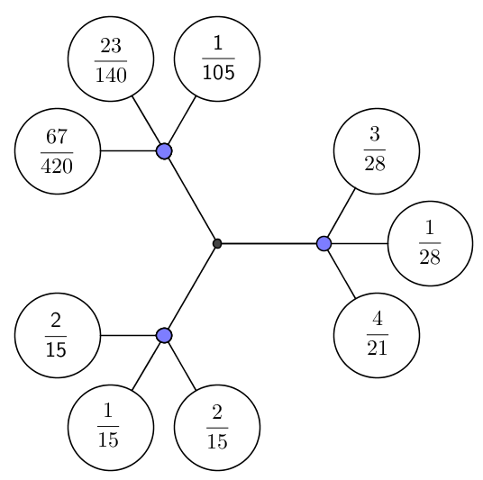
Figure 1: $\mu$

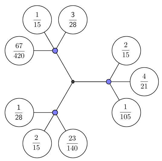
Figure 2: $\nu$

Nevertheless, the signature can be discriminative in some cases. In the following, we give lower bounds for the $L_{1}$-Wasserstein distance between two signatures under three different alternatives.

3.1 When the distances are multiplied by some positive real number $\lambda$

Let $\lambda$ be some positive real number. The DTM-signature discriminates between two mm-spaces isomorphic up to a dilatation of parameter $\lambda$, for $\lambda\neq 1$.

Proposition 12.

Let $(\mathcal{X},\delta,\mu)$ and $(\mathcal{Y},\gamma,\nu)=(\mathcal{X},\lambda\delta,\mu)$ be two mm-spaces. We have

$$W_{1}(\rm d\it_{\mu,m}(\mu),\rm d\it_{\nu,m}(\nu))=|1-\lambda|\,\mathbbm{E}_{\mu}[\rm d\it_{\mu,m}(X)],$$

for $X$ a random variable of law $\mu$.

Proof

First remark that $F^{-1}_{\rm d\it_{\nu,m}(\nu)}=\lambda F^{-1}_{\rm d\it_{\mu,m}(\mu)}$. Then,

$$W_{1}(\rm d\it_{\mu,m}(\mu),\rm d\it_{\nu,m}(\nu)) =\int_{0}^{1}\left|F^{-1}_{\rm d\it_{\mu,m}(\mu)}(s)-F^{-1}_{\rm d\it_{\nu,m}(\nu)}(s)\right|\,\rm d\it s$$

$$=|1-\lambda|\,\int_{0}^{1}\left|F^{-1}_{\rm d\it_{\mu,m}(\mu)}(s)\right|\,\rm d\it s$$

$$=|1-\lambda|\,\mathbbm{E}_{\mu}\left[\rm d\it_{\mu,m}(X)\right].$$

$\blacksquare$

3.2 The case of uniform measures on non-empty bounded open subsets of $\mathbbm{R}^{d}$

The DTM-signature discriminates between two uniform measures over two non-empty bounded open subsets of $\mathbbm{R}^{d}$ with different Lebesgue volume.

Proposition 13.

Let $(O,\|\cdot\|_{2},\mu_{O})$ and $(O^{\prime},\|\cdot\|_{2},\mu_{O^{\prime}})$ be two mm-spaces, for $O$ and $O^{\prime}$ two non-empty bounded open subsets of $\mathbbm{R}^{d}$ satisfying $O=\left(\overline{O}\right)^{\circ}$ and $O^{\prime}=\left({\overline{O^{\prime}}}\right)^{\circ}$, and $\|.\|_{2}$ the euclidean norm. A lower bound for $W_{1}(\rm d\it_{\mu_{O},m}(\mu_{O}),\rm d\it_{\mu_{O^{\prime}},m}(\mu_{O^{\prime}}))$ is given by:

$$\min\left(\mu_{O}\left(O_{\epsilon(m,O)}\right),\mu_{O^{\prime}}\left({O^{\prime}}_{\epsilon(m,O^{\prime})}\right)\right)\frac{d}{d+1}\left(\frac{m}{\omega_{d}}\right)^{\frac{1}{d}}\left|\rm Leb\it_{d}(O)^{\frac{1}{d}}-\rm Leb\it_{d}(O^{\prime})^{\frac{1}{d}}\right|.$$

Here, $O_{\epsilon}=\left\{x\in O\,|\,\rm d\it(x,\partial O)\geq\epsilon\right\},$ and $\epsilon(m,O)=\left(\frac{m\rm Leb\it_{d}(O)}{\omega_{d}}\right)^{\frac{1}{d}}$ is the radius of any ball of $\mu_{O}$ mass $m$, included in $O$.

Proof

If the set $O_{\epsilon(m,O)}$ is non-empty, then the minimal value of the distance to a measure is given by:

$$\min_{x\in\mathbbm{R}^{d}}(\rm d\it_{\mu_{O},m}(x))=\rm d\it_{\min}:=\frac{d}{d+1}\left(\frac{m\rm Leb\it_{d}(O)}{\omega_{d}}\right)^{\frac{1}{d}}.$$

Moreover, the points at minimal distance are exactly the points of $O_{\epsilon(m,O)}$. This is Proposition 25 in the Appendix. So, $F_{\rm d\it_{\mu_{O},m}(\mu_{O})}(\rm d\it_{\min})=\mu_{O}\left({O}_{\epsilon(m,O)}\right)$. To conclude, we use the definition of the $L_{1}$-Wasserstein distance as the $L_{1}$-norm between the cumulative distribution functions. $\blacksquare$

3.3 The case of two measures on the same open subset of $\mathbbm{R}^{d}$ with one measure uniform

Let $(O,\|\cdot\|_{2},\mu_{O})$ and $(O,\|\cdot\|_{2},\nu)$ be two mm-spaces with $O$ a non-empty bounded open subset of $\mathbbm{R}^{d}$ and $\nu$ a measure absolutely continuous with respect to $\mu_{O}$. Thanks to the Radon-Nikodym theorem, there is some $\mu_{O}$-measurable function $f$ on $O$ such that for all Borel set $A$ in $O$:

$$\nu(A)=\int_{A}f(\omega)\rm d\it\mu_{O}(\omega).$$

We can consider the $\lambda$-super-level sets of the function $f$ denoted by $\{f\geq\lambda\}$. As for the previous part, we will denote by $\{f\geq\lambda\}_{\epsilon}$ the set of points belonging to $\{f\geq\lambda\}$ whose distance to $\partial\{f\geq\lambda\}$ is at least $\epsilon$.

Then we get the following lower bound for the $L_{1}$-Wasserstein distance between the two signatures:

Proposition 14.

Under these hypotheses, a lower bound for $W_{1}(\rm d\it_{\mu_{O},m}(\mu_{O}),\rm d\it_{\nu,m}(\nu))$ is given by:

$$\frac{1}{1+d}\frac{1}{\rm Leb\it_{d}(O)}\left(\frac{m\rm Leb\it_{d}(O)}{\omega_{d}}\right)^{\frac{1}{d}}\int_{\lambda=1}^{\infty}\frac{1}{\lambda^{\frac{1}{d}}}\max_{\lambda^{\prime}\geq\lambda}\rm Leb\it_{d}\left(\{f\geq\lambda^{\prime}\}_{\left(\frac{m}{\omega_{d}}\frac{\rm Leb\it_{d}(O)}{\lambda^{\prime}}\right)^{\frac{1}{d}}}\right)\rm d\it\lambda.$$

Proof

Proof in the Appendix, in Section A.2.$\blacksquare$

When the density $f$ is Hölder

We assume that $f$ is Hölder on $O$, with positive parameters $\chi\in(0,1]$ and $L>0$, that is:

$$\forall x,y\in O,\ |f(x)-f(y)|\leq L\|x-y\|_{2}^{\chi}.$$

We also assume that $\rm Reach\it(O)>0$. Then for $m$ small enough, the DTM-signature is discriminative.

Proposition 15.

Under the previous assumptions, if one of the following conditions is satisfied, then the quantity $W_{1}(\rm d\it_{\mu_{O},m}(\mu_{O}),\rm d\it_{\nu,m}(\nu))$ is positive:

$$m<\frac{\omega_{d}}{\rm Leb\it_{d}(O)}\min\left\{\rm Reach\it(O)^{d},\left(\frac{\|f\|_{\infty,O}-1}{2L}\right)^{\frac{d}{\chi}}\right\};$$

$$m\in\left[\frac{\omega_{d}}{\rm Leb\it_{d}(O)}(\rm Reach\it(O))^{d},\left(\|f\|_{\infty,O}-2L(\rm Reach\it(O))^{\chi}\right)(\rm Reach\it(O))^{d}\frac{\omega_{d}}{\rm Leb\it_{d}(O)}\right);$$

$$m\in\left[\frac{\omega_{d}}{\rm Leb\it_{d}(O)}\left(\frac{d}{\chi}\right)^{\frac{d}{\chi}}(2L)^{-\frac{d}{\chi}},\min\left\{m_{0},\frac{\omega_{d}}{\rm Leb\it_{d}(O)}(\rm Reach\it(O))^{d+\chi}\frac{\chi}{d}2L\right\}\right),$$

with $m_{0}=\|f\|_{\infty,O}^{\frac{d}{\chi}+1}\ \frac{\omega_{d}}{\rm Leb\it_{d}(O)}\left(\frac{d}{\chi}\right)^{\frac{d}{\chi}}(2L)^{-\frac{d}{\chi}}\left(\frac{\chi}{d+\chi}\right)^{\frac{\chi}{d+\chi}}$.

Moreover, under any of these conditions, we get the lower bound for the quantity $W_{1}(\rm d\it_{\mu_{O},m}(\mu_{O}),\rm d\it_{\nu,m}(\nu))$:

$$\frac{1}{1+d}\left(\frac{m\rm Leb\it_{d}(O)}{\omega_{d}}\right)^{\frac{1}{d}}\int_{\lambda=1}^{\infty}\frac{1}{\lambda^{1+\frac{1}{d}}}\sup_{\lambda^{\prime}\geq\lambda}\nu\left(\left\{f\geq\lambda^{\prime}+L\epsilon(\lambda^{\prime})^{\chi}\right\}\cap O_{\epsilon(\lambda^{\prime})}\right)\rm d\it\lambda,$$

with $\epsilon(\lambda^{\prime})=\lambda^{\prime-\frac{1}{d}}\left(\frac{m\rm Leb\it_{d}(O)}{\omega_{d}}\right)^{\frac{1}{d}}$.

Proof

Proof in the Appendix, in Section A.2. $\blacksquare$

The previous examples provide several relevant cases where the DTM-signature turns out to be discriminative. It is thus appealing to use it as a tool to compare mm-spaces up to isomorphism.

4 An algorithm to compare metric-measure spaces from samples

In this section, $(\mathcal{X},\delta,\mu)$ and $(\mathcal{Y},\gamma,\nu)$ are two mm-spaces. We build a test of the null hypothesis

$$H_{0}\text{ ``The mm-spaces }(\mathcal{X},\delta,\mu)\text{ and }(\mathcal{Y},\gamma,\nu)\text{ are isomorphic''},$$

against its alternative:

$$H_{1}\text{ ``The mm-spaces }(\mathcal{X},\delta,\mu)\text{ and }(\mathcal{Y},\gamma,\nu)\text{ are not isomorphic''}.$$

4.1 The algorithm

The test we propose is based on the fact that the DTM-signatures associated to two isomorphic mm-spaces are equal. If so, it leads to a pseudo-distance $W_{1}\left(\rm d\it_{\mu,m}(\mu),\rm d\it_{\nu,m}(\nu)\right)$ equal to zero.

Let consider, in this part, a $N$-sample $P$ from the measure $\mu$, and a $N$-sample $Q$ from the measure $\nu$. A natural idea for a test is to approximate the pseudo-distance by the statistic $W_{1}\left(\rm d\it_{\mathbbm{1}_{P},m}(\mathbbm{1}_{P}),\rm d\it_{\mathbbm{1}_{Q},m}(\mathbbm{1}_{Q})\right)$, where $\mathbbm{1}_{P}$ is the uniform probability measure on the set $P$, and to reject the hypothesis $H_{0}$ if this statistic is larger than some critical value. The choice of the critical value should rely on some parameter $\alpha\in(0,1)$ and lead to a level $\alpha$ for the test. It strongly depends on the measures $\mu$ and $\nu$ that are unknown. Nonetheless, there exist classical ways of approximating a critical value, one is to mimic the distribution of the statistic by replacing the distribution $\mu$ with the distribution $\mathbbm{1}_{P}$ and $\nu$ with $\mathbbm{1}_{Q}$. Unfortunately, this standard method known as bootstrap fails theoretically and experimentally for our framework.

Thus, we propose another kind of bootstrap. For this purpose, we need to take $P^{\prime}$ a subset of $P$ and $Q^{\prime}$ a subset of $Q$. The statistic we focus on is $W_{1}\left(\rm d\it_{\mathbbm{1}_{P},m}(\mathbbm{1}_{P^{\prime}}),\rm d\it_{\mathbbm{1}_{Q},m}(\mathbbm{1}_{Q^{\prime}})\right)$. It turns out that in this case, the critical value associated to this statistic can be well approximated from the samples $P$ and $Q$, for a suitable size of $P^{\prime}$ and $Q^{\prime}$ with respect to $N$.

This approach leads to the following algorithm.

Algorithm 1: Test Procedure

⬇

Input:$P$ and $Q$ $N$-samples from $\mu$ (respectively $\nu$), $N$, $n$, $m$, $\alpha$, $N_{MC}$ even;

# Compute $T$ the test statistic

Take $P^{\prime}$ a random subset of $P$ of size $n$;

Take $Q^{\prime}$ a random subset of $Q$ of size $n$;

$T\leftarrow\sqrt{n}W_{1}(\rm d\it_{\mathbbm{1}_{P},m}(\mathbbm{1}_{P^{\prime}}),\rm d\it_{\mathbbm{1}_{Q},m}(\mathbbm{1}_{Q^{\prime}}))$;

# Compute $boot$ a $N_{MC}$-sample from the bootstrap law

$dtmP\leftarrow(\rm d\it_{\mathbbm{1}_{P},m}(x))_{x\in P}$;

$dtmQ\leftarrow(\rm d\it_{\mathbbm{1}_{Q},m}(x))_{x\in Q}$;

Let $boot$ be empty;

for j in 1..$\lfloor N_{MC}/2\rfloor$:

Let $dtmP_{1}$ and $dtmP_{2}$ be two independent $n$-samples from $\mathbbm{1}_{dtmP}$;

Let $dtmQ_{1}$ and $dtmQ_{2}$ be two independent $n$-samples from $\mathbbm{1}_{dtmQ}$;

Add $\sqrt{n}W_{1}(\mathbbm{1}_{dtmP_{1}},\mathbbm{1}_{dtmP_{2}})$ and $\sqrt{n}W_{1}(\mathbbm{1}_{dtmQ_{1}},\mathbbm{1}_{dtmQ_{2}})$ to $boot$;

# Compute $qalph$, the $\alpha$-quantile of $boot$

Let $qalph$ be the $\lfloor N_{MC}-N_{MC}\times\alpha\rfloor$th smallest element of $boot$;

Output:$(T\geq qalph)$

Recall that the $L_{1}$-Wasserstein distance $W_{1}$ is simply the $L_{1}$-norm of the difference between the cumulative distribution functions. It can be implemented by the $\mathtt{R}$ function $\mathtt{emdw}$ from the package $\mathtt{emdist}$. To compute the distance to an empirical measure at a point $x$, it is sufficient to search for its nearest neighbours; see section 2. This can be implemented by the $\mathtt{R}$ function $\mathtt{dtm}$ with tuning parameter $r=1$, from the package $\mathtt{TDA}$ [15].

4.2 Validity of the method

In order to prove the validity of our method, we need to introduce a statistical framework.

First of all, from two $N$-samples from the mm-spaces $(\mathcal{X},\delta,\mu)$ and $(\mathcal{Y},\gamma,\nu)$, we derive four independent empirical measures, $\hat{\mu}_{n}$, $\hat{\mu}_{N-n}$, $\hat{\nu}_{n}$ and $\hat{\nu}_{N-n}$. We also denote $\hat{\mu}_{N}$ (respectively $\hat{\nu}_{N}$) the empirical measure associated to the whole $N$-sample of law $\mu$ (respectively $\nu$), that is $\hat{\mu}_{N}=\frac{n}{N}\hat{\mu}_{n}+\frac{N-n}{N}\hat{\mu}_{N-n}$.

Then, we define the test statistic as:

$$T_{N,n,m}(\mu,\nu)=\sqrt{n}W_{1}\left(\rm d\it_{\hat{\mu}_{N},m}(\hat{\mu}_{n}),\rm d\it_{\hat{\nu}_{N},m}(\hat{\nu}_{n})\right).$$

Its law will be denoted by $\mathcal{L}_{N,n,m}(\mu,\nu)$.

Remark that for two isomorphic mm-spaces $(\mathcal{X},\delta,\mu)$ and $(\mathcal{Y},\gamma,\nu)$, the distribution of $T_{N,n,m}(\mu,\nu)$ is $\mathcal{L}_{N,n,m}(\mu,\mu)$, $\mathcal{L}_{N,n,m}(\nu,\nu)$, but also $\frac{1}{2}\mathcal{L}_{N,n,m}(\mu,\mu)+\frac{1}{2}\mathcal{L}_{N,n,m}(\nu,\nu)$; see Lemma 27 in the Appendix.

For some $\alpha>0$, we denote by $\rm q\it_{\alpha}=\inf\{x\in\mathbbm{R}\,|\,F(x)\geq 1-\alpha\}$, the $\alpha$-quantile of a distribution with cumulative distribution function $F$ .

The $\alpha$-quantile $\rm q\it_{\alpha,N,n}$ of $\frac{1}{2}\mathcal{L}_{N,n,m}(\mu,\mu)+\frac{1}{2}\mathcal{L}_{N,n,m}(\nu,\nu)$ will be approximated by the $\alpha$-quantile $\hat{\rm}q\it_{\alpha,N,n}$ of $\frac{1}{2}\mathcal{L}^{*}_{N,n,m}(\hat{\mu}_{N},\hat{\mu}_{N})+\frac{1}{2}\mathcal{L}^{*}_{N,n,m}(\hat{\nu}_{N},\hat{\nu}_{N})$. Here $\mathcal{L}^{*}_{N,n,m}(\hat{\mu}_{N},\hat{\mu}_{N})$ stands for the distribution of $\sqrt{n}W_{1}\left(\rm d\it_{\hat{\mu}_{N},m}(\mu^{*}_{n}),\rm d\it_{\hat{\mu}_{N},m}(\mu^{\prime*}_{n})\right)$ conditionally to $\hat{\mu}_{N}$, where $\mu^{*}_{n}$ and $\mu^{\prime*}_{n}$ are two empirical measures from independent $n$-samples of law $\hat{\mu}_{N}$.

The test we deal with in this paper is then:

$$\phi_{N}=\mathbbm{1}_{T_{N,n,m}(\mu,\nu)\geq\hat{\rm}q\it_{\alpha,N,n}}.$$

The null hypothesis $H_{0}$ is rejected if $\phi_{N}=1$, that is if the $L_{1}$-Wasserstein distance between the two empirical signatures $\rm d\it_{\hat{\mu}_{N},m}(\hat{\mu}_{n})$ and $\rm d\it_{\hat{\nu}_{N},m}(\hat{\nu}_{n})$ is too high.

4.2.1 A test of asymptotic level $\alpha$

In this part, we prove that the test we propose is of asymptotic level $\alpha$, that is such that:

$$\limsup_{N\rightarrow\infty}\mathbbm{P}_{(\mu,\nu)\in H_{0}}(\phi_{N}=1)\leq\alpha.$$

For this, we prove that the law of the test statistic $\frac{1}{2}\mathcal{L}_{N,n,m}(\mu,\mu)+\frac{1}{2}\mathcal{L}_{N,n,m}(\nu,\nu)$ under the hypothesis $H_{0}$ and the bootstrap law $\frac{1}{2}\mathcal{L}^{*}_{N,n,m}(\hat{\mu}_{N},\hat{\mu}_{N})+\frac{1}{2}\mathcal{L}^{*}_{N,n,m}(\hat{\nu}_{N},\hat{\nu}_{N})$ converge weakly to some fixed distribution when $n$ and $N$ go to $\infty$. In order to adopt a non-asymptotic and more visual point of view, we also derive upper bounds in expectation for the $L_{1}$-Wasserstein distance between these two distributions.

Remark that it is sufficient to prove weak convergence for $\mathcal{L}_{N,n,m}(\mu,\mu)$ and $\mathcal{L}^{*}_{N,n,m}(\hat{\mu}_{N},\hat{\mu}_{N})$. Moreover,

$$W_{1}\left(\frac{1}{2}\mathcal{L}_{N,n,m}(\mu,\mu)+\frac{1}{2}\mathcal{L}_{N,n,m}(\nu,\nu),\frac{1}{2}\mathcal{L}^{*}_{N,n,m}(\hat{\mu}_{N},\hat{\mu}_{N})+\frac{1}{2}\mathcal{L}^{*}_{N,n,m}(\hat{\nu}_{N},\hat{\nu}_{N})\right)$$

is upper bounded by

$$\frac{1}{2}W_{1}\left(\mathcal{L}_{N,n,m}(\mu,\mu),\mathcal{L}^{*}_{N,n,m}(\hat{\mu}_{N},\hat{\mu}_{N})\right)+\frac{1}{2}W_{1}\left(\mathcal{L}_{N,n,m}(\nu,\nu),\mathcal{L}^{*}_{N,n,m}(\hat{\nu}_{N},\hat{\nu}_{N})\right).$$

This is a straightforward consequence of the definition of the $L_{1}$-Wasserstein distance with transport plans. Thus, this is also sufficient to derive upper bounds in expectation for the quantity $W_{1}\left(\mathcal{L}_{N,n,m}(\mu,\mu),\mathcal{L}^{*}_{N,n,m}(\hat{\mu}_{N},\hat{\mu}_{N})\right)$.

Lemma 16.

For $\mu$ a measure supported on a compact set, we choose $n$ as a function of $N$ such that: when $N$ goes to infinity, $n$ goes to infinity, $\sqrt{n}\mathbbm{E}[\|\rm d\it_{\mu,m}-\rm d\it_{\hat{\mu}_{N},m}\|_{\infty,\mathcal{X}}]$ goes to zero or more specifically $\frac{\sqrt{n}}{m}\mathbbm{E}[W_{1}(\mu,\hat{\mu}_{N})]$ goes to zero. Then we have that:

$$\mathcal{L}_{N,n,m}(\mu,\mu)\leadsto\mathcal{L}\left(\|\mathbbm{G}_{\mu,m}-\mathbbm{G}^{\prime}_{\mu,m}\|_{1}\right),$$

when $N$ goes to infinity. Moreover, if $n$ is chosen such that $\sqrt{n}W_{1}(\rm d\it_{\mu,m}(\mu),\rm d\it_{\mu,m}(\hat{\mu}_{N}))$ and $\sqrt{n}\|\rm d\it_{\mu,m}-\rm d\it_{\hat{\mu}_{N},m}\|_{\infty,\mathcal{X}}$ go to zero a.e., we have that for almost every sample $X_{1},X_{2},\ldots X_{N}\ldots$:

$$\mathcal{L}^{*}_{N,n,m}(\hat{\mu}_{N},\hat{\mu}_{N})\leadsto\mathcal{L}\left(\|\mathbbm{G}_{\mu,m}-\mathbbm{G}^{\prime}_{\mu,m}\|_{1}\right),$$

when $N$ goes to infinity; with $\mathbbm{G}_{\mu,m}$ and $\mathbbm{G}^{\prime}_{\mu,m}$ two independent Gaussian processes with covariance kernel $\kappa(s,t)=F_{\rm d\it_{\mu,m}(\mu)}(s)\left(1-F_{\rm d\it_{\mu,m}(\mu)}(t)\right)$ for $s\leq t$.

Proof

Proof in the Appendix, in Section C.3. $\blacksquare$

Proposition 17.

If the two weak convergences in lemma 16 occur, and if the $\alpha$-quantile $\rm q\it_{\alpha}$ of the distribution $\mathcal{L}(\frac{1}{2}\|\mathbbm{G}_{\mu,m}-\mathbbm{G}^{\prime}_{\mu,m}\|_{1}+\frac{1}{2}\|\mathbbm{G}_{\nu,m}-\mathbbm{G}^{\prime}_{\nu,m}\|_{1})$ is a point of continuity of its cumulative distribution function, then the asymptotic level of the test at $(\mu,\nu)$ is $\alpha$.

Proof

Proof in the Appendix, in Section C.3. $\blacksquare$

Remark that for uniform measures on any sphere in $\mathbbm{R}^{d}$, the continuity assumption for the cumulative distribution function of $\mathcal{L}(\|\mathbbm{G}_{\mu,m}-\mathbbm{G}^{\prime}_{\mu,m}\|_{1})$ is not satisfied. This is a degenerated case. Thus, the test cannot be applied to such mm-spaces.

We choose $N=cn^{\rho}$ for some positive constants $\rho$ and $c$. Then the test is asymptotically valid for two measures supported on a compact subset of the Euclidean space $\mathbbm{R}^{d}$ if we assume that $\rho>\frac{\max\{d,2\}}{2}$.

Proposition 18.

Let $\mu$ be some Borel probability measure supported on some compact subset of $\mathbbm{R}^{d}$. Under the assumption

$$\rho>\frac{\max\{d,2\}}{2},$$

the two weak convergences of lemma 16 occur.

Moreover, a bound for the expectation of $W_{1}\left(\mathcal{L}_{N,n,m}(\mu,\mu),\mathcal{L}^{*}_{N,n,m}(\hat{\mu}_{N},\hat{\mu}_{N})\right)$ is of order:

$$N^{\frac{1}{2\rho}-\frac{1}{\max\{d,2\}}}\left(\log(1+N)\right)^{\mathbbm{1}_{d=2}}.$$

And, $W_{1}\left(\mathcal{L}_{N,n,m}(\mu,\mu),\mathcal{L}^{*}_{N,n,m}(\hat{\mu}_{N},\hat{\mu}_{N})\right)\rightarrow 0$ a.e. when $n$ goes to $\infty$.

Proof

This proposition is based on rates of convergence for the Wasserstein distance between a measure $\mu$ with values in $\mathbbm{R}^{d}$ and its empirical version $\hat{\mu}_{N}$; see [17] for general dimensions and [6] for $d=1$. Proof in the Appendix, in Section C.4. $\blacksquare$

A probability measure $\mu$ is $(a,b)$-standard with positive parameters $a$ and $b$, if for all positive radius $r$ and any point $x$ of the support of $\mu$, we have that $\mu(\rm B\it(x,r))\geq\min\{1,ar^{b}\}$. Uniform measures on open subsets of $\mathbbm{R}^{d}$ satisfy such a property:

Example 19.

Let $O$ be a non-empty bounded open subset of $\mathbbm{R}^{d}$. Then, the measure $\mu_{O}$ is $(a,d)$-standard with

$$a=\frac{\omega_{d}}{\rm Leb\it_{d}(O)}\left(\frac{\rm Reach\it(O)}{\mathcal{D}(O)}\right)^{d}.$$

Here, $\mathcal{D}(O)$ stands for the diameter of $O$ and $\omega_{d}$ for $\rm Leb\it_{d}(\rm B\it(0,1))$, the Lebesgue volume of the unit $d$-dimensional ball.

Proof

Proof in the Appendix, in Section A.1. $\blacksquare$

Similar results can be obtained for uniform measures on compact submanifolds of dimension $d$. In [24] (lemma 5.3), the authors give a bound for $a$ depending on the reach of the submanifold.

The test is asymptotically valid for two $(a,b)$-standard measures supported on compact connected subsets of $\mathbbm{R}^{d}$ if $\rho>1$:

Proposition 20.

Let $\mu$ be an $(a,b)$-standard measure supported on a connected compact subset of $\mathbbm{R}^{d}$. The two weak convergences of lemma 16 occur if the assumption $\rho>1$ is satisfied. Moreover, a bound for the expectation of $W_{1}\left(\mathcal{L}_{N,n,m}(\mu,\mu),\mathcal{L}^{*}_{N,n,m}(\hat{\mu}_{N},\hat{\mu}_{N})\right)$ is of order $N^{\frac{1}{2\rho}-\frac{1}{2}}$ up to a logarithm term.

Proof

This proposition is based on rates of convergence for the infinity norm between the distance to a measure and its empirical version; see [13]. Proof in the Appendix, in Section C.5. $\blacksquare$

Remark that we can achieve a rate close to the parametric rate for Ahlfors regular measures, whereas for general measures, the rate gets worse when the dimension increases. Anyway, we need $\rho$ to be as big as possible for the bootstrapped law to be a good enough approximation of the law of the statistic, that is to have a type I error close enough to $\alpha$; keeping in mind that $n$ should go to $\infty$ with $N$.

4.2.2 The power of the test

The power of the test $\phi_{N}=\mathbbm{1}_{\sqrt{n}W_{1}\left(\rm d\it_{\hat{\mu}_{N},m}(\hat{\mu}_{n}),\rm d\it_{\hat{\nu}_{N},m}(\hat{\nu}_{n})\right)\geq\hat{\rm}q\it_{\alpha,N,n}}$ is defined for two mm-spaces $(\mathcal{X},\delta,\mu)$ and $(\mathcal{Y},\gamma,\nu)$ by:

$$1-\mathbbm{P}_{(\mu,\nu)}\left(\phi_{N}=0\right).$$

If the spaces are not isomorphic, we want the test to reject the null with high probability. It means that we want the power to be as big as possible. Here, we give a lower bound for the power, or more precisely an upper bound for $\mathbbm{P}_{(\mu,\nu)}\left(\phi_{N}=0\right)$, the type II error.

Proposition 21.

Let $\mu$ and $\nu$ be two Borel measures supported on $\mathcal{X}$ and $\mathcal{Y}$, two compact subsets of $\mathbbm{R}^{d}$. We assume that the mm-spaces $(\mathcal{X},\delta,\mu)$ and $(\mathcal{Y},\gamma,\nu)$ are non-isomorphic and that the DTM-signature is discriminative for some $m$ in $(0,1]$, that is such that $W_{1}\left(\rm d\it_{\mu,m}(\mu),\rm d\it_{\nu,m}(\nu)\right)>0$. We choose $N=n^{\rho}$ with $\rho>1$. Then for all positive $\epsilon$, there exists $n_{0}$ depending on $\mu$ and $\nu$ such that for all $n\geq n_{0}$, the type II error

$$\mathbbm{P}_{(\mu,\nu)}\left(\sqrt{n}W_{1}\left(\rm d\it_{\hat{\mu}_{N},m}(\hat{\mu}_{n}),\rm d\it_{\hat{\nu}_{N},m}(\hat{\nu}_{n})\right)<\hat{\rm}q\it_{\alpha,N,n}\right)$$

is upper bounded by

$$4\exp\left(-\frac{W_{1}^{2}\left(\rm d\it_{\mu,m}(\mu),\rm d\it_{\nu,m}(\nu)\right)}{(2+\epsilon)\max\left\{\mathcal{D}_{\mu,m}^{2},\mathcal{D}_{\nu,m}^{2}\right\}}n\right),$$

with $\mathcal{D}_{\mu,m}$, the diameter of the support of the measure $\rm d\it_{\mu,m}(\mu)$.

Proof

Proof in the Appendix, in Section C.6. $\blacksquare$

In order to have a high power, that is to reject $H_{0}$ more often when the mm-spaces are not isomorphic, we need $n$ to be big enough, that is $\rho$ small enough. Recall that $n$ has to be small enough for the law of the statistic and its bootstrap version to be close. It means that some compromise should be done. Moreover, the choice of $m$ for the test should depend on the geometry of the mm-spaces. The tuning of these parameters from data is still an open question.

5 Numerical illustrations

Let $\mu_{v}$ be the distribution of the random vector $(R\sin(vR)+0.03N,R\cos(vR)+0.03N^{\prime})$ with $R$, $N$ and $N^{\prime}$ independent random variables; $N$ and $N^{\prime}$ from the standard normal distribution and $R$ uniform on $(0,1)$. With the notation given in the Introduction, we consider the sets $\Theta_{0}=\{(\mu_{10},\mu_{10})\}$ and $\Theta_{1}=\{(\mu_{10},\mu_{p})\,|\,p\neq 10\}$. We sample $N=2000$ points from two measure, choose $\alpha=0.05$, $m=0.05$, $n=20$, and $N_{MC}=1000$. We give an example under which our test (DTM) is working and more powerful than (KS), which consists in applying a Kolmogorov-Smirnov test to $\frac{N}{2}$-samples from $\mathcal{L}(\delta(X,X^{\prime}))$ and $\mathcal{L}(\gamma(Y,Y^{\prime}))$ with $X$ and $X^{\prime}$ (resp. $Y$ and $Y^{\prime}$) independent from $\mu$ (resp. $\nu$). The experiments are repeated 1000 times to approximate the type I error for our test and the power for both tests.

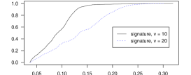
Figure 3: DTM-signature estimates, $m=0.05$

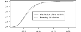
Figure 4: Bootstrap validity, $v=10$, $m=0.05$

v	15	20	30	40	100
type I error DTM	0.050	0.049	0.051	0.044	0.051
power DTM	0.525	0.884	0.987	0.977	0.985
power KS	0.768	0.402	0.465	0.414	0.422

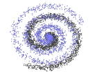
Figure 5: Type I error and power approximations

6 Concluding remarks and perspectives

This paper opens a new horizon of statistical tests based on shape signatures. It could be of interest to adapt these kind of methods to other signatures, if possible. In future it could even be interesting to build statistical tests based on many different signatures, leading to an even better discrimination. Regarding the test proposed in this paper itself, the geometric and statistical problem of the choice of the best parameters to use in practice is still an open, tough and engaging question.

Acknowledgements

The author is extremely grateful to Frédéric Chazal, Pascal Massart and Bertrand Michel for introducing her to the distance to a measure, for their valuable comments and advises, and for proofreading.

Appendix

Appendix A Uniform measures on open subsets of $\mathbbm{R}^{d}$

In this part, we focus on some mm-spaces $(O,\|\cdot\|_{2},\mu_{O})$ where $O$ stands for a non-empty bounded open subset of $\mathbbm{R}^{d}$ satisfying $\left(\overline{O}\right)^{\circ}=O$. The measure $\mu_{O}$, the medial axis $\mathcal{M}(O)$ and the reach $\rm Reach\it(O)$ have been defined in Section 2. The object $\epsilon(m,O)$ is defined for some mass parameter $m$ in $[0,1]$ by

$$\epsilon(m,O)=\left(\frac{m\rm Leb\it_{d}(O)}{\omega_{d}}\right)^{\frac{1}{d}}.$$

This is the radius of a ball included in $O$, with $\mu_{O}$ measure equal to $m$. For some positive $\epsilon$, $O_{\epsilon}$ stands for the set of points in $O$ which distance to $\partial O$ is not smaller than $\epsilon$:

$$O_{\epsilon}=\left\{x\in O,\inf_{y\in\partial O}\|x-y\|_{2}\geq\epsilon\right\}.$$

A.1 The distance to uniform measures

Here, we derive some properties of the spaces $(O,\|\cdot\|_{2},\mu_{O})$. We give a lower bound for the minimum of the distance to the measure $\mu_{O}$ and give a description of the points attaining this bound. Then, we use such considerations to prove identifiability of the measure $\mu_{O}$ from its distance-to-a-measure function. That is, to prove Proposition 7 of the paper.

First, we state some technical lemma proposed by Lieutier in [20].

Lemma 22.

If we define the skeleton $\rm Sk\it(O)$ of the open set $O$ as the set of centres of maximal balls (for the inclusion) included in $O$, then we get:

$$\mathcal{M}(O)\subset\rm Sk\it(O)\subset\overline{\mathcal{M}(O)}.$$

Now we can formulate some technical lemma:

Lemma 23.

For any $x$ in $O$, there exist a maximal ball for the inclusion, included in $O$ and containing $x$.

Proof

Let us consider the class $\mathcal{S}=\{\rm B\it(y,r)\,|\,r>0\text{ and }x\in\rm B\it(y,r)\subset O\}$ of all non-empty open balls included in $O$ and containing $x$. We are going to show that this class contains a maximal element by using the Zorn’s lemma. For this, we need to show that the partially-ordered set $\mathcal{S}$ is inductive, which means that any non-empty totally-ordered subclass $\mathcal{T}$ of $\mathcal{S}$ is upper bounded by some element of $\mathcal{S}$. Let $\mathcal{T}$ be a non-empty totally-ordered subclass of $\mathcal{S}$. Set $R=\sup\{r>0\,|\,\exists\,y\in O,\rm B\it(y,r)\in\mathcal{T}\}$ the supremum of the radii of all balls in $\mathcal{T}$. Since $\mathcal{T}$ is non-empty and $O$ is bounded, $R$ if positive and finite. Let $(y_{k})_{k\in\mathbbm{N}}$ be a sequence of centres of balls in $\mathcal{T}$ converging to a point $y$ in $\mathbbm{R}^{d}$ such that the sequence of associated radii $(r_{k})_{k\in\mathbbm{N}}$ is non decreasing with $R$ as a limit. Since $\mathcal{T}$ is totally-ordered and the radii non decreasing, the union $\bigcup_{k\in\mathbbm{N}}\rm B\it(y_{k},r_{k})$ is non decreasing, equal to $\rm B\it(y,R)$. Thus, $\rm B\it(y,R)$ belongs to $\mathcal{S}$ and upper bounds $\mathcal{T}$. So the class $\mathcal{S}$ is inductive and thanks to the Zorn’s lemma, it contains a maximal element. $\blacksquare$

Proof of Example 19:

For any point $x$ in $O$ and $r>0$, thanks to Lemma 23 there exist a maximal ball $\rm B\it(x^{\prime},r^{\prime})$ included in $O\cap\rm B\it(x,r)$ which contains $x$. Assume for the sake of contradiction that $r^{\prime}<\min\left\{\frac{r}{2},\rm Reach\it(O)\right\}$.

Since $r^{\prime}<\frac{r}{2}$, the ball $\overline{\rm B\it}(x^{\prime},r^{\prime})$ is included in $\rm B\it(x,r)$ thus $\rm B\it(x^{\prime},r^{\prime})$ is maximal in $O$. So $x^{\prime}$ belongs to $\rm Sk\it(O)$, and thanks to Lemma 22, to $\overline{\mathcal{M}(O)}$. But $r^{\prime}<\rm Reach\it(O)$; this is absurd.

It follows that:

$$\mu_{O}(\rm B\it(x,r))\geq\mu_{O}\left(\rm B\it\left(x^{\prime},\min\left\{\rm Reach\it(O),\frac{r}{2}\right\}\right)\right).$$

So, for $r\leq 2\rm Reach\it(O)$, since $2\rm Reach\it(O)\leq\mathcal{D}(O)$ by considering a point on $\rm Sk\it(O)$, we get:

$$\mu_{O}(\rm B\it(x,r))\geq r^{d}\left(\frac{\rm Reach\it(O)}{\mathcal{D}(O)}\right)^{d}\frac{\omega_{d}}{\rm Leb\it_{d}(O)},$$

which is also true for $r$ in $[2\rm Reach\it(O),\mathcal{D}(O)]$, whereas for $r\geq\mathcal{D}(O)$ we have $\mu_{O}(\rm B\it(x,r))=1$. The choice of $a$ in the lemma is thus relevant. $\blacksquare$

We now focus on the set of points in $\mathbbm{R}^{d}$ minimizing the distance to the measure $\mu_{O}$. For this, we need some lemma.

Lemma 24.

If $x$ in $\mathbbm{R}^{d}$ satisfies $\mu_{O}(\rm B\it(x,\epsilon))=\frac{\omega_{d}\epsilon^{d}}{\rm Leb\it_{d}(O)}$, then $\rm B\it(x,\epsilon)\subset O$.

Proof

If $x$ in $\mathbbm{R}^{d}$ satisfies $\mu_{O}(\rm B\it(x,\epsilon))=\frac{\omega_{d}\epsilon^{d}}{\rm Leb\it_{d}(O)}$, then, $\rm Leb\it_{d}(O^{c}\cap\rm B\it(x,\epsilon))=0$. Assume for the sake of contradiction that the set $O^{c}\cap\rm B\it(x,\epsilon)$ is not empty. Since $\left(\overline{O}\right)^{\circ}=O$, then the open subset $\left(O^{c}\right)^{\circ}\cap\rm B\it(x,\epsilon)$ of $O^{c}\cap\rm B\it(x,\epsilon)$ is not empty, thus of positive Lebesgue measure, which is absurd. So $\rm B\it(x,\epsilon)\subset O$. $\blacksquare$

Proposition 25.

The constant $\rm d\it_{\min}=\frac{d}{d+1}\left(\frac{m\rm Leb\it_{d}(O)}{\omega_{d}}\right)^{\frac{1}{d}}$ is a lower bound for the distance to the measure $\mu_{O}$ over $\mathbbm{R}^{d}$. Moreover, the set of points attaining this bound is exactly $O_{\epsilon(m,O)}$.

Proof

Remark that for all positive $l$ smaller than $m$, we have:

$$\delta_{\mu,l}(x)\geq\left(\frac{l\rm Leb\it_{d}(O)}{\omega_{d}}\right)^{\frac{1}{d}}.$$

Moreover, these inequalities are equalities for all points $x$ in $O_{\epsilon(m,O)}$. By integrating, we get the lower bound $\rm d\it_{\min}$ for $x\mapsto\rm d\it_{\mu,m}(x)$, and it is attained on $O_{\epsilon(m,O)}$.

Now take some point $x$ in $\mathbbm{R}^{d}$ satisfying $\rm d\it_{\mu,m}(x)=\rm d\it_{\min}$. For almost all $l$ smaller than $m$, we have: $\delta_{\mu,l}(x)=\left(\frac{l\rm Leb\it_{d}(O)}{\omega_{d}}\right)^{\frac{1}{d}}$. In particular we get for these values of $l$ that:

$$\mu\left(\overline{\rm B\it}\left(x,\left(\frac{m\rm Leb\it_{d}(O)}{\omega_{d}}\right)^{\frac{1}{d}}\right)\right)>l.$$

So, $\mu\left(\rm B\it\left(x,\left(\frac{m\rm Leb\it_{d}(O)}{\omega_{d}}\right)^{\frac{1}{d}}\right)\right)=m$, and thanks to Lemma 24, we get that $x\in O_{\epsilon(m,O)}$. $\blacksquare$

Proposition 26.

If $\rm Reach\it(O)\geq\epsilon(m,O)$, then:

$$\{x\in\mathbbm{R}^{d}\,|\,\rm d\it_{\mu,m}(x)=\rm d\it_{\min}\}^{\epsilon(m,O)}=O,$$

where for any set $A$, the notation $A^{\epsilon}$ stands for $\bigcup_{x\in A}\overline{\rm B\it}(x,\epsilon)$, the $\epsilon$-offset of $A$.

Proof

Remind thanks to Proposition 25 that $\{x\in\mathbbm{R}^{d}\,|\,\rm d\it_{\mu,m}(x)=\rm d\it_{\min}\}=O_{\epsilon(m,O)}$. Moreover, $O_{\epsilon(m,O)}^{\epsilon(m,O)}\subset O$. Assume for the sake of contradiction that the set $O\backslash O_{\epsilon(m,O)}^{\epsilon(m,O)}$ is non-empty. Take a point $x$ in this set and consider $\rm B\it(x^{\prime},r^{\prime})$ a maximal ball containing $x$ and included in $O$ given by Lemma 23. Since $x\notin O_{\epsilon(m,O)}^{\epsilon(m,O)}$, we get that $r^{\prime}<\epsilon(m,O)$. Moreover, $x^{\prime}$ belongs to $\rm Sk\it(O)$ and so, thanks to Lemma 22, to $\overline{\mathcal{M}}(O)$. Then, by continuity of the function distance to the compact set $\partial O$, $r^{\prime}=\rm d\it_{\partial O}(x^{\prime})\geq\rm Reach\it(O)\geq\epsilon(m,O)$, which is a contradiction. So, $O_{\epsilon(m,O)}^{\epsilon(m,O)}=O$. $\blacksquare$

A.2 The DTM-signature to discriminate between uniform and non uniform measures.

Proof of Proposition 14:

As for Proposition 25, we get that for any point $x$ in $O$:

$$\rm d\it_{\mu_{O},m}(x)\geq\rm d\it_{\min}:=\left(\frac{m\rm Leb\it_{d}(O)}{\omega_{d}}\right)^{\frac{1}{d}}\frac{d}{1+d}.$$

We will lower bound the $L_{1}$-Wasserstein distance between $\rm d\it_{\mu_{O},m}(\mu_{O})$ and $\rm d\it_{\nu,m}(\nu)$ by the integral of $F_{\rm d\it_{\nu,m}(\nu)}$ over the interval $[0,\rm d\it_{\min}]$, since $F_{\rm d\it_{\mu_{O},m}(\mu_{O})}$ equals zero on this interval. We thus need to lower bound $F_{\rm d\it_{\nu,m}(\nu)}(t)$ for all $t\leq\rm d\it_{\min}$.

As for Proposition 25, for $\lambda\geq 1$, any point $x$ of $\{f\geq\lambda\}_{\lambda^{-\frac{1}{d}}\left(\frac{m\rm Leb\it_{d}(O)}{\omega_{d}}\right)^{\frac{1}{d}}}$ satisfies $\rm d\it_{\nu,m}(x)\leq\frac{\rm d\it_{\min}}{\lambda^{\frac{1}{d}}}$. Thus,

$$F_{\rm d\it_{\nu,m}(\nu)}\left(\frac{\rm d\it_{\min}}{\lambda^{\frac{1}{d}}}\right)\geq\nu\left(\{f\geq\lambda\}_{\lambda^{-\frac{1}{d}}\left(\frac{m\rm Leb\it_{d}(O)}{\omega_{d}}\right)^{\frac{1}{d}}}\right).$$

And we get by denoting $\lambda(t)$ the real number $\lambda$ satisfying $t=\frac{\rm d\it_{\min}}{\lambda^{\frac{1}{d}}}$, that:

$$W_{1}(\rm d\it_{\mu_{O},m}(\mu_{O}),\rm d\it_{\nu,m}(\nu))\geq\int_{t=0}^{\rm d\it_{\min}}\nu\left(\{f\geq\lambda(t)\}_{\lambda(t)^{-\frac{1}{d}}\left(\frac{m\rm Leb\it_{d}(O)}{\omega_{d}}\right)^{\frac{1}{d}}}\right)\rm d\it t.$$

Since a cumulative distribution function in non decreasing, we get:

$$W_{1}(\rm d\it_{\mu_{O},m}(\mu_{O}),\rm d\it_{\nu,m}(\nu))\geq$$

$$\int_{t=0}^{\rm d\it_{\min}}\sup_{t^{\prime}\leq t}\nu\left(\{f\geq\lambda(t^{\prime})\}_{\lambda(t^{\prime})^{-\frac{1}{d}}\left(\frac{m\rm Leb\it_{d}(O)}{\omega_{d}}\right)^{\frac{1}{d}}}\right)\rm d\it t$$

$$=\int_{\lambda=1}^{\infty}\rm d\it_{\min}\frac{1}{d}\frac{1}{\lambda^{\frac{1}{d}}}\frac{1}{\lambda}\sup_{\lambda^{\prime}\geq\lambda}\nu\left(\{f\geq\lambda^{\prime}\}_{\lambda^{\prime-\frac{1}{d}}\left(\frac{m\rm Leb\it_{d}(O)}{\omega_{d}}\right)^{\frac{1}{d}}}\right)\rm d\it\lambda$$

$$\geq\frac{1}{d+1}\left(\frac{m\rm Leb\it_{d}(O)}{\omega_{d}}\right)^{\frac{1}{d}}\int_{\lambda=1}^{\infty}\frac{1}{\lambda^{\frac{1}{d}}}\sup_{\lambda^{\prime}\geq\lambda}\mu_{O}\left(\{f\geq\lambda^{\prime}\}_{\left(\frac{m\rm Leb\it_{d}(O)}{\lambda^{\prime}\omega_{d}}\right)^{\frac{1}{d}}}\right)\rm d\it\lambda.$$

$\blacksquare$

Now we assume that the density $f$ is Hölder over $O$ with parameters $\chi$ in $[0,1]$ and $L$ in $\mathbbm{R}_{+}^{*}$.

Proof of Proposition 15:

First remark that for all positive $\lambda$, with $\epsilon(\lambda)=\lambda^{-\frac{1}{d}}\left(\frac{m\rm Leb\it_{d}(O)}{\omega_{d}}\right)^{\frac{1}{d}}$ we have:

$$\left\{f\geq\lambda+L\epsilon(\lambda)^{\chi}\right\}\cap O_{\epsilon(\lambda)}\subset\{f\geq\lambda\}_{\epsilon(\lambda)}.$$

According to Proposition 14, the aim is thus to show that for some $\lambda$ bigger than 1, the set $\left\{f\geq\lambda+L\epsilon(\lambda)^{\chi}\right\}\cap O_{\epsilon(\lambda)}$ is non-empty. We thus focus on the supremum of $f$ over $O_{\epsilon(\lambda)}$, which we denote by $\|f\|_{\infty,\epsilon(\lambda)}$.

Remind that if $\rm Reach\it(O)\geq\epsilon(\lambda)$, then thanks to Proposition 26, the set $O_{\epsilon(\lambda)}^{\epsilon(\lambda)}$ equals $O$. Since $f$ is Hölder, we can thus build some sequence $(y_{n})_{n\in\mathbbm{N}^{*}}$ in $O_{\epsilon(\lambda)}$, such that $f(y_{n})\geq\|f\|_{\infty,O}-\frac{1}{n}-L\epsilon(\lambda)^{\chi}$. Finally we get:

$$\|f\|_{\infty,\epsilon(\lambda)}\geq\|f\|_{\infty,O}-L\epsilon(\lambda)^{\chi}.$$

So the quantity $W_{1}(\rm d\it_{\mu_{O},m}(\mu_{O}),\rm d\it_{\nu,m}(\nu))$ is positive whenever:

$$\|f\|_{\infty,O}>\inf\left\{\lambda+2L\epsilon(\lambda)^{\chi}\,|\,\lambda\geq 1,\epsilon(\lambda)\leq\rm Reach\it(O)\right\}.$$

With $\lambda_{0}=1$, we have $\lambda_{0}+2L\epsilon(\lambda_{0})^{\chi}=1+2L\left(\frac{m\rm Leb\it_{d}(O)}{\omega_{d}}\right)^{\frac{\chi}{d}}$.

With $\lambda_{1}$ satisfying $\epsilon(\lambda_{1})=\rm Reach\it(O)$, we have:

$$\lambda_{1}+2L\epsilon(\lambda_{1})^{\chi}=\frac{1}{(\rm Reach\it(O))^{d}}\frac{m\rm Leb\it_{d}(O)}{\omega_{d}}+2L(\rm Reach\it(O)^{\chi}).$$

We also have that

$$\inf\left\{\lambda+2L\epsilon(\lambda)^{\chi}\,|\,\lambda>0\right\}=(2L)^{\frac{d}{d+\chi}}\left(\frac{\rm Leb\it_{d}(O)}{\omega_{d}}\right)^{\frac{\chi}{d+\chi}}m^{\frac{\chi}{d+\chi}}\left[\left(\frac{\chi}{d}\right)^{\frac{d}{\chi+d}}+\left(\frac{\chi}{d}\right)^{-\frac{\chi}{d+\chi}}\right].$$

The infimum is attained at $\lambda_{2}=\left(\frac{\chi}{d}\right)^{\frac{d}{\chi+d}}(2L)^{\frac{d}{\chi+d}}\left(\frac{m\rm Leb\it_{d}(O)}{\omega_{d}}\right)^{\frac{\chi}{\chi+d}}$.

It proves the first part of the proposition.

The second part is a straightforward consequence of the proof of Proposition 14. $\blacksquare$

Appendix B Stability of the DTM-signature

Proof of Proposition 9:

The proof is relatively similar to the ones given by Mémoli in [23] for other signatures.

For any map plan $\pi$ between $\mu$ and $\nu$ Borel measures on $(\mathcal{X},\delta)$ and $(\mathcal{Y},\gamma)$, we get:

$$W_{1}(\rm d\it_{\mu,m}(\mu),\rm d\it_{\nu,m}(\nu))\leq$$

$$\int_{\mathcal{X}\times\mathcal{Y}}\left|\rm d\it_{\mu,m}(x)-\rm d\it_{\nu,m}(y)\right|\rm d\it\pi(x,y)=$$

$$\int_{\mathcal{X}\times\mathcal{Y}}\left|\frac{1}{m}\int_{0}^{m}\delta_{\mu,l}(x)\rm d\it l-\frac{1}{m}\int_{0}^{m}\delta_{\nu,l}(y)\rm d\it l\right|\rm d\it\pi(x,y)\leq$$

$$\int_{\mathcal{X}\times\mathcal{Y}}\frac{1}{m}\int_{0}^{m}\left|\delta_{\mu,l}(x)-\delta_{\nu,l}(y)\right|\rm d\it l\,\rm d\it\pi(x,y)=$$

$$\frac{1}{m}\int_{\mathcal{X}\times\mathcal{Y}}\int_{0}^{m}\left|\inf\{r>0\,|\,\mu(\overline{\rm B\it}(x,r))>l\}-\inf\{r>0\,|\,\nu(\overline{\rm B\it}(y,r))>l\}\right|\rm d\it l\,\rm d\it\pi(x,y)=$$

$$\frac{1}{m}\int_{\mathcal{X}\times\mathcal{Y}}\int_{0}^{m}\left|\int_{0}^{+\infty}\left(\mathbbm{1}_{\mu(\overline{\rm B\it}(x,r))\leq l}-\mathbbm{1}_{\nu(\overline{\rm B\it}(y,r))\leq l}\right)\rm d\it r\right|\rm d\it l\,\rm d\it\pi(x,y)\leq$$

$$\frac{1}{m}\int_{\mathcal{X}\times\mathcal{Y}}\int_{0}^{+\infty}\int_{0}^{m}\left|\mathbbm{1}_{\mu(\overline{\rm B\it}(x,r))\leq l}-\mathbbm{1}_{\nu(\overline{\rm B\it}(y,r))\leq l}\right|\rm d\it l\,\rm d\it r\,\rm d\it\pi(x,y)\leq$$

$$\frac{1}{m}\int_{\mathcal{X}\times\mathcal{Y}}\int_{0}^{+\infty}\left|\mu(\overline{\rm B\it}(x,r))\wedge m-\nu(\overline{\rm B\it}(y,r))\wedge m\right|\rm d\it r\,\rm d\it\pi(x,y)\leq$$

$$\frac{1}{m}\int_{\mathcal{X}\times\mathcal{Y}}\int_{0}^{+\infty}\left|\int_{\mathcal{X}\times\mathcal{Y}}\left(\mathbbm{1}_{\delta(x,x^{\prime})\leq r}-\mathbbm{1}_{\gamma(y,y^{\prime})\leq r}\right)\rm d\it\pi(x^{\prime},y^{\prime})\right|\wedge m\,\rm d\it r\,\rm d\it\pi(x,y)\leq$$

$$\frac{1}{m}\int_{\mathcal{X}\times\mathcal{Y}}\int_{\mathcal{X}\times\mathcal{Y}}\int_{0}^{+\infty}\left|\mathbbm{1}_{\delta(x,x^{\prime})\leq r}-\mathbbm{1}_{\gamma(y,y^{\prime})\leq r}\right|\rm d\it r\,\rm d\it\pi(x^{\prime},y^{\prime})\,\rm d\it\pi(x,y)=$$

$$\frac{1}{m}\int_{\mathcal{X}\times\mathcal{Y}}\int_{\mathcal{X}\times\mathcal{Y}}\left|\delta(x,x^{\prime})-\gamma(y,y^{\prime})\right|\rm d\it\pi(x^{\prime},y^{\prime})\,\rm d\it\pi(x,y),$$

which concludes.

Appendix C The test

C.1 A lemma

Lemma 27 (Equality of empirical signatures under the isomorphic assumption).

If $(\mathcal{X},\delta,\mu)$ and $(\mathcal{Y},\gamma,\nu)$ are two isomorphic mm-spaces, then the distributions of the random variables

$$\sqrt{n}W_{1}(\rm d\it_{\hat{\mu}_{N},m}(\hat{\mu}_{n}),\rm d\it_{\hat{\mu}^{\prime}_{N},m}(\hat{\mu}^{\prime}_{n}))$$

and

$$\sqrt{n}W_{1}(\rm d\it_{\hat{\mu}_{N},m}(\hat{\mu}_{n}),\rm d\it_{\hat{\nu}_{N},m}(\hat{\nu}_{n}))$$

are equal. Here the empirical measures are all independent and the measures $\hat{\mu}^{\prime}_{N}$ and $\hat{\mu}^{\prime}_{n}$ are from samples from $\mu$.

Proof

Remark that for $(X^{\prime}_{1},X^{\prime}_{2},\ldots,X^{\prime}_{N})$ a $N$-sample of law $\mu$ and $\phi$ an isomorphism between $(\mathcal{X},\delta,\mu)$ and $(\mathcal{Y},\gamma,\nu)$, the tuple $(\phi(X^{\prime}_{1}),\phi(X^{\prime}_{2}),\ldots,\phi(X^{\prime}_{N}))$ is a $N$-sample of law $\nu$. Moreover, $\delta(X^{\prime}_{i},X^{\prime}_{j})=\gamma(\phi(X^{\prime}_{i}),\phi(X^{\prime}_{j}))$ for all $i$ and $j$ in $[\![1,N]\!]$. It follows that the distances and the nearest neighbours are preserved.

Thus, the distributions of $(\rm d\it_{\hat{\mu}_{N},m}(X^{\prime}_{i}))_{i\in[\![1,n]\!]}$ and $(\rm d\it_{\hat{\nu}_{N},m}(Y_{i}))_{i\in[\![1,n]\!]}$ are equal.

The lemma follows from the equality:

$$W_{1}(\rm d\it_{\hat{\mu}_{N},m}(\hat{\mu}_{n}),\rm d\it_{\hat{\nu}_{N},m}(\hat{\nu}_{n}))$$

$$=\int_{0}^{+\infty}\frac{1}{n}\left|\sum_{i=1}^{n}\mathbbm{1}_{\rm d\it_{\hat{\mu}_{N},m}(X_{i})\leq s}-\sum_{i=1}^{n}\mathbbm{1}_{\rm d\it_{\hat{\nu}_{N},m}(Y_{i})\leq s}\right|\rm d\it s,$$

with $(X_{1},X_{2},\ldots,X_{N})$ a $N$-sample from $\mu$. $\blacksquare$

C.2 $L_{1}$-Wasserstein distance between the laws of interest

Lemma 28.

The quantity $W_{1}\left(\mathcal{L}_{N,n,m}(\mu,\mu),\mathcal{L}^{*}_{N,n,m}(\hat{\mu}_{N},\hat{\mu}_{N})\right)$ is upper bounded by:

$$2\sqrt{n}\left(\mathbbm{E}[\|\rm d\it_{\hat{\mu}_{N},m}-\rm d\it_{\mu,m}\|_{\infty,\mathcal{X}}]+W_{1}(\rm d\it_{\mu,m}(\mu),\rm d\it_{\mu,m}(\hat{\mu}_{N}))+\|\rm d\it_{\mu,m}-\rm d\it_{\hat{\mu}_{N},m}\|_{\infty,\mathcal{X}}\right).$$

Proof

Let $(X_{1},X_{2},\ldots X_{N})$ be a $N$-sample of law $\mu$, and $\hat{\mu}_{N}$ the associated empirical measure. We can upper bound the $L_{1}$-Wasserstein distance between the bootstrap law $\mathcal{L}^{*}(\sqrt{n}W_{1}(\rm d\it_{\hat{\mu}_{N},m}(\mu^{*}_{n}),\rm d\it_{\hat{\mu}_{N},m}(\mu^{\prime*}_{n}))|\hat{\mu}_{N})$ and the law of interest $\mathcal{L}(\sqrt{n}W_{1}(\rm d\it_{\hat{\mu}_{N},m}(\hat{\mu}_{n}),\rm d\it_{\hat{\mu}^{\prime}_{N},m}(\hat{\mu}^{\prime}_{n})))$, by:

$$W_{1}\left(\mathcal{L}\left(\sqrt{n}W_{1}\left(\rm d\it_{\hat{\mu}_{N},m}\left(\mu^{*}_{n}\right),\rm d\it_{\hat{\mu}_{N},m}\left(\mu^{\prime*}_{n}\right)\right)|\hat{\mu}_{N}\right),\mathcal{L}\left(\sqrt{n}W_{1}\left(\rm d\it_{\mu,m}\left(\mu^{*}_{n}\right),\rm d\it_{\mu,m}\left(\mu^{\prime*}_{n}\right)\right)|\hat{\mu}_{N}\right)\right)$$ (1)

$$+W_{1}\left(\mathcal{L}\left(\sqrt{n}W_{1}\left(\rm d\it_{\mu,m}\left(\mu^{*}_{n}\right),\rm d\it_{\mu,m}\left(\mu^{\prime*}_{n}\right)\right)|\hat{\mu}_{N}\right),\mathcal{L}\left(\sqrt{n}W_{1}\left(\rm d\it_{\mu,m}\left(\hat{\mu}_{n}\right),\rm d\it_{\mu,m}\left(\hat{\mu}^{\prime}_{n}\right)\right)\right)\right)$$ (2)

$$+W_{1}\left(\mathcal{L}\left(\sqrt{n}W_{1}\left(\rm d\it_{\mu,m}\left(\hat{\mu}_{n}\right),\rm d\it_{\mu,m}\left(\hat{\mu}^{\prime}_{n}\right)\right)\right),\mathcal{L}\left(\sqrt{n}W_{1}\left(\rm d\it_{\hat{\mu}_{N},m}\left(\hat{\mu}_{n}\right),\rm d\it_{\hat{\mu}^{\prime}_{N},m}\left(\hat{\mu}^{\prime}_{n}\right)\right)\right)\right).$$ (3)

We bound the term 1 by:

$$2\sqrt{n}\|\rm d\it_{\mu,m}-\rm d\it_{\hat{\mu}_{N},m}\|_{\infty,\mathcal{X}}.$$

the term 2 by

$$2\sqrt{n}W_{1}\left(\rm d\it_{\mu,m}(\mu),\rm d\it_{\mu,m}\left(\hat{\mu}_{N}\right)\right)$$

and the term 3 by

$$2\sqrt{n}\mathbbm{E}[\|\rm d\it_{\mu,m}-\rm d\it_{\hat{\mu}_{N},m}\|_{\infty,\mathcal{X}}].$$

This is proved in the three following lemmata. $\blacksquare$

Lemma 29 (Study of term 3).

We have

$$W_{1}\left(\mathcal{L}(\sqrt{n}W_{1}(\rm d\it_{\hat{\mu}_{N},m}(\hat{\mu}_{n}),\rm d\it_{\hat{\mu}^{\prime}_{N},m}(\hat{\mu}^{\prime}_{n}))),\mathcal{L}(\sqrt{n}W_{1}(\rm d\it_{\mu,m}(\hat{\mu}_{n}),\rm d\it_{\mu,m}(\hat{\mu}^{\prime}_{n})))\right)\leq$$

$$2\sqrt{n}\mathbbm{E}[\|\rm d\it_{\mu,m}-\rm d\it_{\hat{\mu}_{N},m}\|_{\infty,\mathcal{X}}].$$

Proof

To bound this $L_{1}$-Wasserstein distance, we choose as a transport plan the law of the random vector

$$(\sqrt{n}W_{1}(\rm d\it_{\hat{\mu}_{N},m}(\hat{\mu}_{n}),\rm d\it_{\hat{\mu}^{\prime}_{N},m}(\hat{\mu}^{\prime}_{n})),\sqrt{n}W_{1}(\rm d\it_{\mu,m}(\hat{\mu}_{n}),\rm d\it_{\mu,m}(\hat{\mu}^{\prime}_{n}))),$$

with $\hat{\mu}_{n}$, $\hat{\mu}^{\prime}_{n}$, $\hat{\mu}_{N-n}$ and $\hat{\mu}^{\prime}_{N-n}$ independent empirical measures of law $\mu$. Then the $L_{1}$-Wasserstein distance is bounded by:

$$\mathbbm{E}[|\sqrt{n}W_{1}(\rm d\it_{\hat{\mu}_{N},m}(\hat{\mu}_{n}),\rm d\it_{\hat{\mu}^{\prime}_{N},m}(\hat{\mu}^{\prime}_{n}))-\sqrt{n}W_{1}(\rm d\it_{\mu,m}(\hat{\mu}_{n}),\rm d\it_{\mu,m}(\hat{\mu}^{\prime}_{n}))|],$$

which is not bigger than:

$$\sqrt{n}\mathbbm{E}[W_{1}(\rm d\it_{\hat{\mu}_{N},m}(\hat{\mu}_{n}),\rm d\it_{\mu,m}(\hat{\mu}_{n}))+W_{1}(\rm d\it_{\hat{\mu}^{\prime}_{N},m}(\hat{\mu}^{\prime}_{n}),\rm d\it_{\mu,m}(\hat{\mu}^{\prime}_{n}))].$$

We bound the term $\mathbbm{E}[W_{1}(\rm d\it_{\hat{\mu}_{N},m}(\hat{\mu}_{n}),\rm d\it_{\mu,m}(\hat{\mu}_{n}))]$ by $\mathbbm{E}[\|\rm d\it_{\mu,m}-\rm d\it_{\hat{\mu}_{N},m}\|_{\infty,\mathcal{X}}]$, thanks to Lemma 32. $\blacksquare$

Lemma 30 (Study of term 2).

We have

$$W_{1}\left(\mathcal{L}(\sqrt{n}W_{1}(\rm d\it_{\mu,m}(\hat{\mu}_{n}),\rm d\it_{\mu,m}(\hat{\mu}^{\prime}_{n})),\mathcal{L}(\sqrt{n}W_{1}(\rm d\it_{\mu,m}(\mu^{*}_{n}),\rm d\it_{\mu,m}(\mu^{\prime*}_{n}))|\hat{\mu}_{N})\right)\leq$$

$$2\sqrt{n}W_{1}(\rm d\it_{\mu,m}(\mu),\rm d\it_{\mu,m}(\hat{\mu}_{N})).$$

Proof

Let $\pi$ be the optimal transport plan associated to $W_{1}\left(\rm d\it_{\mu,m}(\mu),\rm d\it_{\mu,m}(\hat{\mu}_{N})\right)$; see the definition of the $L_{1}$-Wasserstein with transport plans.

From a $n$-sample of law $\pi$, we get two empirical distributions $\rm d\it_{\mu,m}(\hat{\mu}_{n})$ and $\rm d\it_{\mu,m}(\mu^{*}_{n})$. Independently, from another $n$-sample of law $\pi$, we get $\rm d\it_{\mu,m}(\hat{\mu}^{\prime}_{n})$ and $\rm d\it_{\mu,m}(\mu^{\prime*}_{n})$.

The $L_{1}$-Wasserstein distance is then bounded by:

$$\sqrt{n}\mathbbm{E}_{\pi^{\otimes n}\otimes\pi^{\otimes n}}[W_{1}(\rm d\it_{\mu,m}(\hat{\mu}_{n}),\rm d\it_{\mu,m}(\mu^{*}_{n}))+W_{1}(\rm d\it_{\mu,m}(\hat{\mu}^{\prime}_{n}),\rm d\it_{\mu,m}(\mu^{\prime*}_{n}))].$$

Now remark that, if we denote $\hat{\mu}_{n}=\sum_{i=1}^{n}\frac{1}{n}\delta_{Y_{i}}$ and $\mu^{*}_{n}=\sum_{i=1}^{n}\frac{1}{n}\delta_{Z_{i}}$, we have:

$$W_{1}(\rm d\it_{\mu,m}(\hat{\mu}_{n}),\rm d\it_{\mu,m}(\mu^{*}_{n})) =\int_{t=0}^{+\infty}\left|\frac{1}{n}\sum_{i=1}^{n}\mathbbm{1}_{\rm d\it_{\mu,m}(Y_{i})\leq t}-\frac{1}{n}\sum_{i=1}^{n}\mathbbm{1}_{\rm d\it_{\mu,m}(Z_{i})\leq t}\right|\rm d\it t$$

$$\leq\frac{1}{n}\sum_{i=1}^{n}\int_{t=0}^{+\infty}\left|\mathbbm{1}_{\rm d\it_{\mu,m}(Y_{i})\leq t}-\mathbbm{1}_{\rm d\it_{\mu,m}(Z_{i})\leq t}\right|\rm d\it t$$

$$=\frac{1}{n}\sum_{i=1}^{n}\left|\rm d\it_{\mu,m}(Y_{i})-\rm d\it_{\mu,m}(Z_{i})\right|.$$

So, the $L_{1}$-Wasserstein distance is not bigger than

$$2\sqrt{n}\mathbbm{E}[|\rm d\it_{\mu,m}(Y)-\rm d\it_{\mu,m}(Z)|],$$

with $(\rm d\it_{\mu,m}(Y),\rm d\it_{\mu,m}(Z))$ of law $\pi$, so we get the upper bound:

$$2\sqrt{n}\left(W_{1}(\rm d\it_{\mu,m}(\mu),\rm d\it_{\mu,m}(\hat{\mu}_{N})\right).$$

$\blacksquare$

Lemma 31 (Study of term 1).

We have

$$W_{1}\left(\mathcal{L}(\sqrt{n}W_{1}(\rm d\it_{\mu,m}(\mu^{*}_{n}),\rm d\it_{\mu,m}(\mu^{\prime*}_{n}))|\hat{\mu}_{N}),\mathcal{L}(\sqrt{n}W_{1}(\rm d\it_{\hat{\mu}_{N},m}(\mu^{*}_{n}),\rm d\it_{\hat{\mu}_{N},m}(\mu^{\prime*}_{n}))|\hat{\mu}_{N})\right)\leq$$

$$2\sqrt{n}\|\rm d\it_{\mu,m}-\rm d\it_{\hat{\mu}_{N},m}\|_{\infty,\mathcal{X}}.$$

Proof

It is the same proof as for the first lemma, except that $\hat{\mu}_{N}$ is fixed. $\blacksquare$

Lemma 32.

Let $\nu$, $\mu$ and $\mu^{\prime}$ be some measures over some metric space $(\mathcal{X},\delta)$, we have:

$$W_{1}(\rm d\it_{\mu,m}(\nu),\rm d\it_{\mu^{\prime},m}(\nu))\leq\int_{\mathcal{X}}|\rm d\it_{\mu,m}(x)-\rm d\it_{\mu^{\prime},m}(x)|\rm d\it\nu(x)\leq\|\rm d\it_{\mu,m}-\rm d\it_{\mu^{\prime},m}\|_{\infty,\rm Supp\it(\nu)}.$$

Proof

We chose the transport plan $(\rm d\it_{\mu,m}(Y),\rm d\it_{\mu^{\prime},m}(Y))$ for $Y$ of law $\nu$. $\blacksquare$

Thanks to Proposition 5 and to the fact that the distance to a measure is 1-Lipschitz, we can derive another upper bound depending only on the $L_{1}$-Wasserstein distance between the measure $\mu$ and its empirical versions:

Corollary 33.

The quantity $W_{1}\left(\mathcal{L}_{N,n,m}(\mu,\mu),\mathcal{L}^{*}_{N,n,m}(\hat{\mu}_{N},\hat{\mu}_{N})\right)$ is upper bounded by:

$$2\frac{\sqrt{n}}{m}\mathbbm{E}\left[W_{1}\left(\hat{\mu}_{N},\mu\right)\right]+2\sqrt{n}\left(1+\frac{1}{m}\right)W_{1}(\hat{\mu}_{N},\mu).$$

The rates of convergence of the $L_{1}$-Wasserstein distance between a Borel probability measure on the Euclidean space $\mathbbm{R}^{d}$ and its empirical version are faster when the dimension $d$ is low; see [17]. Thus, we prefer to use the first bound for regular measures. In this case, we use rates of convergence for the distance to a measure, derived in [13]. For regular measures, in some cases, the bound in Lemma 28 is better than the bound in Corollary 33.

C.3 An asymptotic result with the convergence to the law of $\|\mathbbm{G}_{\mu,m}-\mathbbm{G}^{\prime}_{\mu,m}\|_{1}$

Proof of Lemma 16:

The random function $\sqrt{n}\left(F_{\rm d\it_{\mu,m}(\mu)}-F_{\rm d\it_{\mu,m}(\hat{\mu}_{n})}\right)$ converges weakly in $L_{1}$ to some gaussian prossess $\mathbbm{G}_{\mu,m}$ with covariance kernel $\kappa(s,t)=F_{\rm d\it_{\mu,m}(\mu)}(s)\left(1-F_{\rm d\it_{\mu,m}(\mu)}(t)\right)$ for $s\leq t$; see [3] or part 3.3 of [6]. Thanks to Theorem 2.8 in [5], since $L_{1}\times L_{1}$ is separable and $\hat{\mu}_{n}$ and $\hat{\mu}^{\prime}_{n}$ are independent, the random vector

$$\left(\sqrt{n}\left(F_{\rm d\it_{\mu,m}(\mu)}-F_{\rm d\it_{\mu,m}(\hat{\mu}_{n})}\right),\sqrt{n}\left(F_{\rm d\it_{\mu,m}(\mu)}-F_{\rm d\it_{\mu,m}(\hat{\mu}^{\prime}_{n})}\right)\right)$$

converges weakly to $(\mathbbm{G}_{\mu,m},\mathbbm{G}^{\prime}_{\mu,m})$ with $\mathbbm{G}_{\mu,m}$ and $\mathbbm{G}^{\prime}_{\mu,m}$ independent Gaussian processes. Since the map $(x,y)\mapsto x-y$ is continuous in $L_{1}$, the mapping theorem states that $\sqrt{n}\left(F_{\rm d\it_{\mu,m}(\hat{\mu}^{\prime}_{n})}-F_{\rm d\it_{\mu,m}(\hat{\mu}_{n})}\right)$ converges weakly to the Gaussian process $\mathbbm{G}_{\mu,m}-\mathbbm{G}^{\prime}_{\mu,m}$ in $L_{1}$. Once more we use the mapping theorem with the continuous map $x\mapsto\|x\|_{1}$ and the definition of the $L_{1}$-Wasserstein distance as the $L_{1}$-norm of the cumulative distribution functions to get that:

$$\sqrt{n}W_{1}(\rm d\it_{\mu,m}(\hat{\mu}_{n}),\rm d\it_{\mu,m}(\hat{\mu}^{\prime}_{n}))\leadsto\|\mathbbm{G}_{\mu,m}-\mathbbm{G}^{\prime}_{\mu,m}\|_{1}.$$

We then get the convergence of moments following the same method as for Theorem 2.4 in [3]. We have the bound $\mathbbm{E}[\|t\mapsto\mathbbm{1}_{\rm d\it_{\mu,m}(X_{i})\leq t}-\mathbbm{1}_{\rm d\it_{\mu,m}(Y_{i})\leq t}\|_{1}]\leq\mathcal{D}_{\mu}<\infty$. Moreover, the random function $\sqrt{n}\left(F_{\rm d\it_{\mu,m}(\hat{\mu}^{\prime}_{n})}-F_{\rm d\it_{\mu,m}(\hat{\mu}_{n})}\right)$ converges weakly to the gaussian process $\mathbbm{G}_{\mu,m}-\mathbbm{G}^{\prime}_{\mu,m}$ in $L_{1}$. So, thanks to Theorem 5.1 in [1] (cited in [2] p.136), we have:

$$\mathbbm{E}[\sqrt{n}W_{1}(\rm d\it_{\mu,m}(\hat{\mu}_{n}),\rm d\it_{\mu,m}(\hat{\mu}^{\prime}_{n}))]\rightarrow\mathbbm{E}[\|\mathbbm{G}_{\mu,m}-\mathbbm{G}^{\prime}_{\mu,m}\|_{1}].$$

We deduce that:

$$W_{1}\left(\mathcal{L}\left(\sqrt{n}W_{1}\left(\rm d\it_{\mu,m}\left(\hat{\mu}_{n}\right),\rm d\it_{\mu,m}\left(\hat{\mu}^{\prime}_{n}\right)\right)\right),\mathcal{L}\left(\|\mathbbm{G}_{\mu,m}-\mathbbm{G}^{\prime}_{\mu,m}\|_{1}\right)\right)\rightarrow 0.$$

Moreover, we have the bound:

$$W_{1}\left(\mathcal{L}\left(\sqrt{n}W_{1}\left(\rm d\it_{\mu,m}\left(\hat{\mu}_{n}\right),\rm d\it_{\mu,m}\left(\hat{\mu}^{\prime}_{n}\right)\right)\right),\mathcal{L}_{N,n,m}(\mu,\mu)\right)\leq 2\sqrt{n}\mathbbm{E}[\|\rm d\it_{\mu,m}-\rm d\it_{\hat{\mu}_{N},m}\|_{\infty,\mathcal{X}}].$$

So, if $\sqrt{n}\mathbbm{E}\left[\|\rm d\it_{\mu,m}-\rm d\it_{\hat{\mu}_{N},m}\|_{\infty,\mathcal{X}}\right]\rightarrow 0$ when $N\rightarrow\infty$, we have that:

$$W_{1}\left(\mathcal{L}_{N,n,m}(\mu,\mu),\mathcal{L}\left(\|\mathbbm{G}_{\mu,m}-\mathbbm{G}^{\prime}_{\mu,m}\|_{1}\right)\right)\rightarrow 0.$$

Finally, with the same arguments as for Lemma 28, we get that:

$$W_{1}\left(\mathcal{L}^{*}_{N,n,m}(\hat{\mu}_{N},\hat{\mu}_{N}),\mathcal{L}\left(\|\mathbbm{G}_{\mu,m}-\mathbbm{G}^{\prime}_{\mu,m}\|_{1}\right)\right)\leq$$

$$W_{1}\left(\mathcal{L}\left(\sqrt{n}W_{1}\left(\rm d\it_{\mu,m}\left(\hat{\mu}_{n}\right),\rm d\it_{\mu,m}\left(\hat{\mu}^{\prime}_{n}\right)\right)\right),\mathcal{L}\left(\|\mathbbm{G}_{\mu,m}-\mathbbm{G}^{\prime}_{\mu,m}\|_{1}\right)\right)$$

$$+2\sqrt{n}W_{1}\left(\rm d\it_{\mu,m}(\mu),\rm d\it_{\mu,m}\left(\hat{\mu}_{N}\right)\right)+2\sqrt{n}\|\rm d\it_{\mu,m}-\rm d\it_{\hat{\mu}_{N},m}\|_{\infty,\mathcal{X}}.$$

$\blacksquare$

Proof of Proposition 17:

Let $\epsilon<\alpha$ and $\eta$ be two positive numbers.

The probability $\mathbbm{P}_{(\mu,\nu)}\left(\phi_{N}=1\right)$ is upper bounded by

$$\mathbbm{P}\left(\sqrt{n}W_{1}\left(\rm d\it_{\hat{\mu}_{N},m}(\hat{\mu}_{n}),\rm d\it_{\hat{\nu}_{N},m}(\hat{\nu}_{n})\right)\geq\rm q\it_{\alpha+\epsilon}-\eta\right)+\mathbbm{P}\left(\hat{\rm}q\it_{\alpha}<\rm q\it_{\alpha+\epsilon}-\eta\right).$$

With a drawing, we see that $\mathbbm{P}\left(\hat{\rm}q\it_{\alpha}<\rm q\it_{\alpha+\epsilon}-\eta\right)$ is upper bounded by

$$\mathbbm{P}\left(W_{1}\left(\mathcal{L}\left(\frac{1}{2}\|\mathbbm{G}_{\mu,m}-\mathbbm{G}^{\prime}_{\mu,m}\|_{1}+\frac{1}{2}\|\mathbbm{G}_{\nu,m}-\mathbbm{G}^{\prime}_{\nu,m}\|_{1}\right),\mathcal{L}^{*}\right)\geq\epsilon\eta\right),$$

where $\mathcal{L}^{*}=\frac{1}{2}\mathcal{L}^{*}_{N,n,m}(\hat{\mu}_{N},\hat{\mu}_{N})+\frac{1}{2}\mathcal{L}^{*}_{N,n,m}(\hat{\nu}_{N},\hat{\nu}_{N})$.

Thanks to the weak convergences in Lemma 16 of the paper and the Portmanteau lemma, $\limsup_{N\rightarrow\infty}\mathbbm{P}_{(\mu,\nu)}\left(\phi_{N}=1\right)$ is thus upper bounded by

$$\mathbbm{P}\left(\frac{1}{2}\|\mathbbm{G}_{\mu,m}-\mathbbm{G}^{\prime}_{\mu,m}\|_{1}+\frac{1}{2}\|\mathbbm{G}_{\nu,m}-\mathbbm{G}^{\prime}_{\nu,m}\|_{1}\geq\rm q\it_{\alpha+\epsilon}-\eta\right).$$

We now make $\eta$ and $\epsilon$ go to zero and under the continuity assumption, $\limsup_{N\rightarrow\infty}\mathbbm{P}_{(\mu,\nu)}\left(\phi_{N}=1\right)\leq\alpha$.

As well, we get that $\liminf_{N\rightarrow\infty}\mathbbm{P}_{(\mu,\nu)}\left(\phi_{N}=1\right)\geq\alpha$.

C.4 The case of measures supported on a compact subset of $\mathbbm{R}^{d}$

Proof of part 2 of Proposition 18:

We may assume that the diameter $\mathcal{D}_{\mu}$ of the support of the measure $\mu$ equals 1. Indeed, if we apply a dilatation to the measure to make the diameter of its support be equal to 1, then the quantity $W_{1}\left(\mathcal{L}_{N,n,m}(\mu,\mu),\mathcal{L}^{*}_{N,n,m}(\hat{\mu}_{N},\hat{\mu}_{N})\right)$ is simply multiplied by the parameter of the dilatation. By using Corollary 33 and Theorem 1 of [17], we have a bound for the expectation:

$$\mathbbm{E}\left[W_{1}\left(\mathcal{L}_{N,n,m}(\mu,\mu),\mathcal{L}^{*}_{N,n,m}(\hat{\mu}_{N},\hat{\mu}_{N})\right)\right]\leq\begin{cases}C\frac{\sqrt{n}}{m}N^{-\frac{1}{d}}&\text{ if d>2}\\ C\frac{\sqrt{n}}{m}N^{-\frac{1}{2}}\log(1+N)&\text{ if d=2}\\ C\frac{\sqrt{n}}{m}N^{-\frac{1}{2}}&\text{ if d<2}\\ \end{cases}$$

for some positive constant $C$ depending on $\mu$. $\blacksquare$

Proof of part 3 of Proposition 18:

First remark that for $\lambda>1$,

$$\mathbbm{P}\left(W_{1}\left(\mathcal{L}_{N,n,m}(\mu,\mu),\mathcal{L}^{*}_{N,n,m}(\hat{\mu}_{N},\hat{\mu}_{N})\right)\geq\lambda\right)=0$$

under the assumption $\mathcal{D}_{\mu}=1$. We thus focus on values of $\lambda$ not bigger than 1. In this case, with the Theorem 2 of [17], we get easily that:

$$\mathbbm{P} \left(W_{1}\left(\mathcal{L}_{N,n,m}(\mu,\mu),\mathcal{L}^{*}_{N,n,m}(\hat{\mu}_{N},\hat{\mu}_{N})\right)\geq\lambda\right)\leq$$

$$\begin{cases}C\exp\left(-C^{\prime}\left(\lambda\frac{N^{\frac{1}{d}}m}{\sqrt{n}}-C^{\prime\prime}\right)^{d}\right)&\text{ for d>2}\\ C\exp\left(-C^{\prime}\left(\frac{\frac{\sqrt{N}m}{\sqrt{n}}\lambda-C^{\prime\prime}\sqrt{\frac{N}{N-n}}\log(1+N-n)}{\log\left(2+\frac{2\sqrt{N}}{\frac{\sqrt{N}m}{\sqrt{n}}\lambda-C^{\prime\prime}\sqrt{\frac{N}{N-n}}\log(1+N-n)}\right)}\right)^{2}\right)&\text{ for d=2}\\ C\exp\left(-C^{\prime}\left(\lambda\frac{\sqrt{N}m}{\sqrt{n}}-C^{\prime\prime}\right)^{2}\right)&\text{ for d<2}\\ \end{cases}$$

for some positive constants $C$, $C^{\prime}$ and $C^{\prime\prime}$ depending on $\mu$.

We conclude the proof with the Borel–Cantelli lemma. $\blacksquare$

Proof of part 1 of Proposition 18:

We need to show that under the assumption $\rho>\frac{\max\{d,2\}}{2}$, the following properties are satisfied:

$$\sqrt{n}\mathbbm{E}[\|\rm d\it_{\mu,m}-\rm d\it_{\hat{\mu}_{N},m}\|_{\infty,\mathcal{X}}]\rightarrow 0,$$

$$\sqrt{n}W_{1}(\rm d\it_{\mu,m}(\mu),\rm d\it_{\mu,m}(\hat{\mu}_{N}))\rightarrow 0\text{ a.e.},$$

and

$$\sqrt{n}\|\rm d\it_{\mu,m}-\rm d\it_{\hat{\mu}_{N},m}\|_{\infty,\mathcal{X}}\rightarrow 0\text{ a.e.}.$$

We treat the case $d>2$. The cases $d<2$ and $d=2$ are similar.

Thanks to Theorem 1 of [17], there is some positive constant $C$ depending on $\mu$ such that for $N$ big enough:

$$\mathbbm{E}[W_{1}(\hat{\mu}_{N},\mu)]\leq C{N}^{-\frac{1}{d}}.$$

Thus, thanks to part 2 of Proposition 18, the quantity $\sqrt{n}\mathbbm{E}[\|\rm d\it_{\mu,m}-\rm d\it_{\hat{\mu}_{N},m}\|_{\infty,\mathcal{X}}]$ goes to zero if $\frac{\sqrt{n}}{m}N^{-\frac{1}{d}}$ goes to zero when $N$ goes to infinity. So, this convergence occurs under the assumption $\rho>\frac{d}{2}$.

We get from Theorem 2 of [17] that for $x\leq 1$, there are some positive constants $C$ and $c$ depending on $\mu$ such that:

$$\mathbbm{P}(W_{1}(\hat{\mu}_{N},\mu)\geq x)\leq C\exp(-cNx^{d}).$$

We use this inequality with $x=\frac{m}{\sqrt{n}}\frac{1}{K}$ for positive integers $K$. Thanks to the Borel–Cantelli lemma, under the assumption $\rho>\frac{d}{2}$, we get that:

$$\frac{\sqrt{n}}{m}W_{1}(\mu,\hat{\mu}_{N})\rightarrow 0\text{ a.e.}.$$

So, thanks to Proposition 5, the third property is true.

To finish, remark that $\rm d\it_{\mu,m}(\hat{\mu}_{N})$ is the empirical measure associated to $\rm d\it_{\mu,m}(\mu)$. Once more we use Theorem 2 of [17] and get that for $x\leq 1$, $\mathbbm{P}(\sqrt{n}W_{1}(\rm d\it_{\mu,m}(\hat{\mu}_{N}),\rm d\it_{\mu,m}(\mu))\geq x)\leq C\exp(-c\frac{N}{n}x^{2})$. Thanks to the Borel–Cantelli lemma, under the assumption $\rho>1$, the a.e. convergence to zero of $\sqrt{n}W_{1}\left(\rm d\it_{\mu,m}(\mu),\rm d\it_{\mu,m}\left(\hat{\mu}_{N}\right)\right)$ occurs. $\blacksquare$

C.5 The case of $(a,b)$-standard measures

Let $\mu$ be a Borel probability measure supported on a connected compact subset $\mathcal{X}$ of $\mathbbm{R}^{d}$. We assume this measure to be $(a,b)$-standard for some positive numbers $a$ and $b$. In this part, we derive rates of convergence in probability and in expectation for the quantity $\|\rm d\it_{\hat{\mu}_{N},m}-\rm d\it_{\mu,m}\|_{\infty,\mathcal{X}}$. Thanks to these results, we can derive upper bounds and rates of convergence in expectation for $W_{1}\left(\mathcal{L}_{N,n,m}(\mu,\mu),\mathcal{L}^{*}_{N,n,m}(\hat{\mu}_{N},\hat{\mu}_{N})\right)$. We finally propose a choice for the parameter $N$ depending on $n$ for which the weak convergences $\mathcal{L}_{N,n,m}(\mu,\mu)\leadsto\|\mathbbm{G}_{\mu,m}-\mathbbm{G}^{\prime}_{\mu,m}\|_{1}$ and $\mathcal{L}^{*}_{N,n,m}(\hat{\mu}_{N},\hat{\mu}^{\prime}_{N})\leadsto\|\mathbbm{G}_{\mu,m}-\mathbbm{G}^{\prime}_{\mu,m}\|_{1}$ occur.

C.5.1 Upper bounds for $\mathbbm{P}(\sqrt{n}\|\rm d\it_{\hat{\mu}_{N},m}-\rm d\it_{\mu,m}\|_{\infty,\mathcal{X}}\geq\lambda)$

We use the bounds given in Theorem 1 of [13], with the bound for the modulus of continuity given by Lemma 3 in [13]: $\omega(h)=\left(\frac{h}{a}\right)^{\frac{1}{b}}$. We directly get the following lemma:

Lemma 34 (Upper bound for $|\rm d\it_{\hat{\mu}_{N},m}(x)-\rm d\it_{\mu,m}(x)|$).

Let $x$ be a fixed point in $\mathcal{X}$ and $\lambda$ a positive number. We have,

$$\frac{1}{2}\mathbbm{P}(|\rm d\it_{\hat{\mu}_{N},m}(x)-\rm d\it_{\mu,m}(x)|\geq\lambda)\leq$$

$$\exp\left(-2a^{\frac{2}{b}}Nm^{\frac{2b-2}{b}}\lambda^{2}\right)+\exp\left(-\frac{a}{2^{b-1}}N^{\frac{b+1}{2}}m^{b}\lambda^{b}\right)+\exp\left(-a^{\frac{1}{b}}N^{\frac{b+1}{2b}}m\lambda\right).$$

In order to derive an upper bound for $\|\rm d\it_{\hat{\mu}_{N},m}-\rm d\it_{\mu,m}\|_{\infty,\mathcal{X}}$, like in [13], we use the fact that the function distance to a measure is 1-Lipschitz and that $\mathcal{X}$ is compact, which means that we can compute a bound by upper-bounding the difference $|\rm d\it_{\hat{\mu}_{N},m}(x)-\rm d\it_{\mu,m}(x)|$ over a finite number of points $x$ of $\mathcal{X}$. Thanks to the following lemma, the minimal number of points needed for this purpose is not bigger than $\frac{(4\mathcal{D}_{\mu}\sqrt{d}+\lambda)^{d}}{\lambda^{d}}$:

Lemma 35.

Let $\mu$ is a measure supported on $\mathcal{X}$ a compact subset of $\mathbbm{R}^{d}$, and for $\lambda>0$ denote $N\left(\mu,\lambda\right)=\inf\{N\in\mathbbm{N},\ \exists\ x_{1},x_{2}\ldots x_{N}\in\mathcal{X},\ \bigcup_{i\in[\![1,N]\!]}\rm B\it(x_{i},\lambda)\supset\mathcal{X}\}$. Then, we have:

$$N\left(\mu,\lambda\right)\leq\frac{\left(\mathcal{D}_{\mu}\sqrt{d}+\lambda\right)^{d}}{\lambda^{d}}.$$

Proof

The idea is to put a grid on the hypercube containing $\mathcal{X}$ with edges of length $\mathcal{D}_{\mu}$. The grid is a union of small hypercubes with edges of length equal to $\frac{\lambda}{\sqrt{d}}$, so that the number of such small hypercubes into which the big one is split is not superior to $\left(\frac{\mathcal{D}_{\mu}\sqrt{d}}{\lambda}+1\right)^{d}$.

Then, we decide that each time the intersection between $\mathcal{X}$ and some small hypercube is non-empty, we keep one of the elements of the intersection. We denote $x_{i}$ the element associated to the $i$-th hypercube. Finally, each point $x$ in $\mathcal{X}$ belongs to a small hypercube, and its distance to the corresponding $x_{i}$ is smaller than $\sqrt{\sum_{k=1}^{d}\frac{\lambda^{2}}{d}}=\lambda$. $\blacksquare$

We thus derive upper bounds for $\sqrt{n}\|\rm d\it_{\hat{\mu}_{N},m}-\rm d\it_{\mu,m}\|_{\infty,\mathcal{X}}$:

Proposition 36 (Upper bound for $\sqrt{n}\|\rm d\it_{\hat{\mu}_{N},m}-\rm d\it_{\mu,m}\|_{\infty,\mathcal{X}}$).

We have,

$$\frac{\lambda^{d}}{2\left(4\mathcal{D}_{\mu}\sqrt{d}+\lambda\right)^{d}}\ \mathbbm{P}(\sqrt{n}\|\rm d\it_{\hat{\mu}_{N},m}-\rm d\it_{\mu,m}\|_{\infty,\mathcal{X}}\geq\lambda)\leq$$

$$\exp\left(-\frac{a^{\frac{2}{b}}}{2}\frac{Nm^{\frac{2b-2}{b}}}{n}\lambda^{2}\right)+\exp\left(-\frac{a}{2^{2b-1}}\frac{N^{\frac{b+1}{2}}m^{b}}{n^{\frac{b}{2}}}\lambda^{b}\right)+\exp\left(-\frac{a^{\frac{1}{b}}}{2}\frac{N^{\frac{b+1}{2b}}m}{n^{\frac{1}{2}}}\lambda\right).$$

Proof

Since the function distance to a measure is 1-Lipschitz, we get that:

$$\|\rm d\it_{\hat{\mu}_{N},m}-\rm d\it_{\mu,m}\|_{\infty,\mathcal{X}}\leq\frac{\lambda}{2}+\sup_{i}\{|\rm d\it_{\hat{\mu}_{N},m}(x_{i})-\rm d\it_{\mu,m}(x_{i})|\},$$

for the family $(x_{i})_{i}$ associated to a grid which sides are of length equal to $\frac{\lambda}{4\sqrt{d}}$. We can thus bound the probability $\mathbbm{P}(\|\rm d\it_{\hat{\mu}_{N},m}-\rm d\it_{\mu,m}\|_{\infty,\mathcal{X}}\geq\lambda)$ by:

$$\sum_{i=1}^{N\left(\mu,\frac{\lambda}{4}\right)}\mathbbm{P}\left(|\rm d\it_{\hat{\mu}_{N},m}(x_{i})-\rm d\it_{\mu,m}(x_{i})|\geq\frac{\lambda}{2}\right),$$

with $N\left(\mu,\frac{\lambda}{4}\right)\leq\frac{\left(4\mathcal{D}_{\mu}\sqrt{d}+\lambda\right)^{d}}{\lambda^{d}}$ thanks to Lemma 35. $\blacksquare$

C.5.2 Upper bounds for the expectation $\mathbbm{E}[\|\rm d\it_{\hat{\mu}_{N},m}-\rm d\it_{\mu,m}\|_{\infty,\mathcal{X}}]$

In order to get upper bounds for $\mathbbm{E}[\|\rm d\it_{\hat{\mu}_{N},m}-\rm d\it_{\mu,m}\|_{\infty,\mathcal{X}}]$, we use the same trick as used in [13], which is:

Lemma 37.

Let $X$ a random variable such that:

$$\mathbbm{P}(X\geq\lambda)\leq 1\wedge D\lambda^{-q}\exp(-c\lambda^{s})$$

for some integers $q$ and $s$ and some $D>0$.

We have:

$$\mathbbm{E}[X]\leq\left(\frac{\ln c}{c}\right)^{\frac{1}{s}}\left(\frac{q}{s}\right)^{\frac{1}{s}}\left[1+D\left(\frac{q}{s}\right)^{\frac{-q-s}{s}}\frac{(\ln c)^{\frac{-q-s}{s}}}{s}\right].$$

More particularly, if $c\geq\exp{D^{\frac{s}{q+s}}\frac{s}{q}}$, then:

$$\mathbbm{E}[X]\leq 2\left(\frac{\ln c}{c}\right)^{\frac{1}{s}}\left(\frac{q}{s}\right)^{\frac{1}{s}}.$$

Proof

For any $\lambda_{0}>0$, that we can choose as $\lambda_{0}=\frac{[\ln K]^{\frac{1}{s}}}{c^{\frac{1}{s}}}$, we get that:

$$\mathbbm{E}[X]\leq\lambda_{0}+\int_{\lambda_{0}}^{\infty}D\lambda^{-q}\exp(-c\lambda^{s})\rm d\it\lambda$$

$$\leq\lambda_{0}+D\frac{\lambda_{0}^{-q-s+1}}{cs}\exp{-c\lambda_{0}^{s}}$$

$$=\frac{[\ln K]^{\frac{1}{s}}}{c^{\frac{1}{s}}}+D\frac{[\ln K]^{\frac{-q-s+1}{s}}}{scc^{\frac{-q-s+1}{s}}}\frac{1}{K}$$

$$=\frac{[\ln K]^{\frac{1}{s}}}{c^{\frac{1}{s}}}+\frac{[\ln K]^{\frac{1}{s}}}{c^{\frac{1}{s}}}D\frac{[\ln K]^{\frac{-q-s}{s}}}{sc^{\frac{-q}{s}}}\frac{1}{K}$$

$$=\frac{[\ln K]^{\frac{1}{s}}}{c^{\frac{1}{s}}}\left[1+D\frac{[\ln K]^{\frac{-q-s}{s}}}{sKc^{\frac{-q}{s}}}\right]$$

Finally, if we choose $K=c^{\frac{q}{s}}$, we get:

$$\mathbbm{E}[X]\leq\left(\frac{q}{s}\right)^{\frac{1}{s}}\left[\frac{\ln c}{c}\right]^{\frac{1}{s}}\left[1+D\left[\frac{q}{s}\right]^{\frac{-q-s}{s}}\frac{(\ln c)^{\frac{-q-s}{s}}}{s}\right].$$

$\blacksquare$

From this lemma, we can derive the following lemma.

Lemma 38.

We have,

$$\mathbbm{E}[\sqrt{n}\|\rm d\it_{\hat{\mu}_{N},m}-\rm d\it_{\mu,m}\|_{\infty,\mathcal{X}}]\leq$$

$$\Box^{\prime}_{1}\frac{n^{\frac{1}{2}}}{N^{\frac{1}{2}}m^{\frac{b-1}{b}}}\left(\log\left(\frac{Nm^{\frac{2b-2}{b}}}{n}\right)\right)^{\frac{1}{2}}+$$

$$\Box^{\prime}_{2}\frac{n^{\frac{1}{2}}}{N^{\frac{b+1}{2b}}m}\left(\log\left(\frac{N^{\frac{b+1}{2}}m^{b}}{n^{\frac{b}{2}}}\right)\right)^{\frac{1}{b}}+$$

$$\Box^{\prime}_{3}\frac{n^{\frac{1}{2}}}{N^{\frac{b+1}{2b}}m}\log\left(\frac{N^{\frac{b+1}{2b}}m}{n^{\frac{1}{2}}}\right).$$

for some constants $\Box$ depending on $a$ and $b$.

C.5.3 Upper bounds for the expectation of $W_{1}\left(\mathcal{L}_{N,n,m}(\mu,\mu),\mathcal{L}^{*}_{N,n,m}(\hat{\mu}_{N},\hat{\mu}_{N})\right)$

Proof of part 2 of Proposition 20:

For all $\lambda>0$, for any measure $\mu$ Ahlfors $b$-regular with parameters $(a,\infty)$ supported on a connected compact subset of $\mathbbm{R}^{d}$, we can use Lemma 28 and Lemma 38 together with the rates of convergence of the $L_{1}$-Wasserstein distance between empirical and true distribution in [6] to get the following result.

If $m\geq\frac{1}{2}$, then for $n$ big enough we have, for some constants $\Box$ depending on $a$ and $b$:

$$\mathbbm{E} \left[W_{1}\left(\mathcal{L}_{N,n,m}(\mu,\mu),\mathcal{L}^{*}_{N,n,m}(\hat{\mu}_{N},\hat{\mu}_{N})\right)\right]\leq$$

$$\Box^{\prime}_{1}\frac{n^{\frac{1}{2}}}{{(N)}^{\frac{1}{2}}m^{\frac{b-1}{b}}}\left(\log\left(\frac{Nm^{\frac{2b-2}{b}}}{n}\right)\right)^{\frac{1}{2}}$$

$$+\Box^{\prime}_{2}\frac{n^{\frac{1}{2}}}{{(N)}^{\frac{b+1}{2b}}m}\left(\log\left(\frac{N^{\frac{b+1}{2}}m^{b}}{n^{\frac{b}{2}}}\right)\right)^{\frac{1}{b}}$$

$$+\Box^{\prime}_{3}\frac{n^{\frac{1}{2}}}{{(N)}^{\frac{b+1}{2b}}m}\log\left(\frac{N^{\frac{b+1}{2b}}m}{n^{\frac{1}{2}}}\right)$$

$$+\Box^{\prime}_{4}\frac{n^{\frac{1}{2}}}{N^{\frac{1}{2}}}.$$

C.5.4 Convergence to the law of $\|\mathbbm{G}_{\mu,m}-\mathbbm{G}^{\prime}_{\mu,m}\|_{1}$

Proof of part 1 of Proposition 20:

In order to get these two results, we use Lemma 16. The convergence to zero of $\sqrt{n}\mathbbm{E}[\|\rm d\it_{\mu,m}-\rm d\it_{\hat{\mu}_{N-n},m}\|_{\infty,\mathcal{X}}]$ is a direct consequence of Lemma 38. We can derive a bound of its rate of convergence in $n^{\frac{1}{2}-\frac{\rho}{2}}$, up to a logarithm term. The a.e. convergence of $\sqrt{n}W_{1}(\rm d\it_{\mu,m}(\mu),\rm d\it_{\mu,m}(\hat{\mu}_{N}))$ to zero is derived as in the proof of Proposition 18, with the assumption $\rho>1$. Finally, the a.e. convergence of $\sqrt{n}\|\rm d\it_{\mu,m}-\rm d\it_{\hat{\mu}_{N},m}\|_{\infty,\mathcal{X}}$ to zero is a consequence of Proposition 36 and of the Borel–Cantelli lemma. It occurs under the assumption $\rho>1$. $\blacksquare$

C.6 The power of the test

Proof of Proposition 21

Lemma 39.

Let $\alpha$, $\kappa$ be two positive numbers and $\mathcal{L}$ and $\mathcal{L}^{*}$ two laws of real random variables. We denote $\rm q\it_{\alpha}$ (respectively $\rm q\it_{\alpha}^{*}$) the $\alpha$-quantile of the law $\mathcal{L}$ (respectively $\mathcal{L}^{*}$). If $W_{1}(\mathcal{L},\mathcal{L}^{*})<\kappa$ then:

$$\rm q\it_{\alpha}^{*}\leq 2\frac{\kappa}{\alpha}+\rm q\it_{\frac{\alpha}{2}}.$$

Proof

With a drawing, since the $L_{1}$-norm between $F_{\mathcal{L}}$ and $F_{\mathcal{L}^{*}}$ is smaller than $\kappa$, we have:

$$F_{\mathcal{L}^{*}}\left(\rm q\it_{\frac{\alpha}{2}}+2\frac{\kappa}{\alpha}\right)>1-\alpha.$$

$\blacksquare$

In this part we assume that $m$ is fixed in $[0,1]$ and $N=cn^{\rho}$ for some $\rho>1$ and $c>0$.

Recall that our aim is to upper bound the type II error, that is:

$$\mathbbm{P}_{(\mu,\nu)}\left(\sqrt{n}W_{1}\left(\rm d\it_{\hat{\mu}_{N},m}(\hat{\mu}_{n}),\rm d\it_{\hat{\nu}_{N},m}(\hat{\nu}_{n})\right)<\hat{\rm}q\it_{\alpha}\right).$$

For some $\kappa=n^{\gamma}$ with $\gamma$ in $\left[0,\frac{1}{2}\right)$ to be chosen later, we first upper bound the quantile $\hat{\rm}q\it_{\alpha}$ with high probability.

As noticed in the proof of Lemma 16, the law of $\sqrt{n}W_{1}\left(\rm d\it_{\mu,m}(\hat{\mu}_{n}),\rm d\it_{\mu,m}(\hat{\mu}^{\prime}_{n})\right)$ converges to $\mathcal{L}(\|\mathbbm{G}_{\mu,m}-\mathbbm{G}^{\prime}_{\mu,m}\|_{1})$, there is also the convergence of the first moments. So, for $n$ big enough, we have:

$$W_{1}(\mathcal{L}\left(\sqrt{n}W_{1}\left(\rm d\it_{\mu,m}(\hat{\mu}_{n}),\rm d\it_{\mu,m}(\hat{\mu}^{\prime}_{n})\right)\right),\mathcal{L}(\|\mathbbm{G}_{\mu,m}-\mathbbm{G}^{\prime}_{\mu,m}\|_{1}))\leq 1.$$

Then, under the assumption

$$W_{1}(\mathcal{L}\left(\sqrt{n}W_{1}\left(\rm d\it_{\mu,m}(\hat{\mu}_{n}),\rm d\it_{\mu,m}(\hat{\mu}^{\prime}_{n})\right)\right),\mathcal{L}^{*}_{N,n,m}(\hat{\mu}_{N},\hat{\mu}_{N}))\leq\kappa,$$

we have

$$W_{1}(\mathcal{L}(\|\mathbbm{G}_{\mu,m}-\mathbbm{G}^{\prime}_{\mu,m}\|_{1}),\mathcal{L}^{*}_{N,n,m}(\hat{\mu}_{N},\hat{\mu}_{N}))\leq\kappa+1.$$

We can do the same thing for $\nu$. Thus we get that for $n$ big enough and under the previous assumptions:

$$W_{1}\left(\frac{1}{2}\mathcal{L}(\|\mathbbm{G}_{\mu,m}-\mathbbm{G}^{\prime}_{\mu,m}\|_{1})+\frac{1}{2}\mathcal{L}(\|\mathbbm{G}_{\nu,m}-\mathbbm{G}^{\prime}_{\nu,m}\|_{1}),\frac{1}{2}\mathcal{L}^{*}_{N,n,m}(\hat{\mu}_{N},\hat{\mu}_{N})+\frac{1}{2}\mathcal{L}^{*}_{N,n,m}(\hat{\nu}_{N},\hat{\nu}_{N})\right)\leq\kappa+1.$$

And thanks to Lemma 39,

$$\hat{\rm}q\it_{\alpha}\leq\tilde{\rm}q\it_{\frac{\alpha}{2}}+2\frac{\kappa+1}{\alpha},$$

with $\tilde{\rm}q\it_{\alpha}$ the $\alpha$-quantile of the law $\frac{1}{2}\mathcal{L}(\|\mathbbm{G}_{\mu,m}-\mathbbm{G}^{\prime}_{\mu,m}\|_{1})+\frac{1}{2}\mathcal{L}(\|\mathbbm{G}_{\nu,m}-\mathbbm{G}^{\prime}_{\nu,m}\|_{1})$.

We need to remark that with similar arguments as for Lemma 28, we have:

$$W_{1}\left(\mathcal{L}\left(\sqrt{n}W_{1}\left(\rm d\it_{\mu,m}(\hat{\mu}_{n}),\rm d\it_{\mu,m}(\hat{\mu}^{\prime}_{n})\right)\right),\mathcal{L}^{*}_{N,n,m}(\hat{\mu}_{N},\hat{\mu}_{N})\right)\leq$$

$$2\sqrt{n}\mathcal{D}_{\mu}\|F_{\rm d\it_{\mu,m}(\mu)}-F_{\rm d\it_{\mu,m}(\hat{\mu}_{N})}\|_{\infty,(0,\mathcal{D}_{\mu})}+2\frac{\sqrt{n}}{m}W_{1}(\mu,\hat{\mu}_{N}).$$

Now remark that

$$\sqrt{n}W_{1}\left(\rm d\it_{\hat{\mu}_{N},m}(\hat{\mu}_{n}),\rm d\it_{\hat{\nu}_{N},m}(\hat{\nu}_{n})\right)\geq\sqrt{n}W_{1}\left(\rm d\it_{\mu,m}(\mu),\rm d\it_{\nu,m}(\nu)\right)$$

$$-\sqrt{n}W_{1}\left(\rm d\it_{\hat{\mu}_{N},m}(\hat{\mu}_{n}),\rm d\it_{\mu,m}(\mu)\right)-\sqrt{n}W_{1}\left(\rm d\it_{\hat{\nu}_{N},m}(\hat{\nu}_{n}),\rm d\it_{\nu,m}(\nu)\right),$$

but as well, thanks to Lemma 32, the definition of the $L_{1}$-Wasserstein distance as the $L_{1}$-norm between the cumulative distribution functions and to Proposition 5:

$$\sqrt{n}W_{1}\left(\rm d\it_{\hat{\mu}_{N},m}(\hat{\mu}_{n}),\rm d\it_{\mu,m}(\mu)\right)\leq$$

$$\frac{\sqrt{n}}{m}W_{1}(\mu,\hat{\mu}_{N})+\sqrt{n}\mathcal{D}_{\mu,m}\|F_{\rm d\it_{\mu,m}(\hat{\mu}_{n})}-F_{\rm d\it_{\mu,m}(\mu)}\|_{\infty,(0,\mathcal{D}_{\mu})},$$

with $\mathcal{D}_{\mu,m}$ the diameter of the support of the measure $\rm d\it_{\mu,m}(\mu)$. So, we can finally upper bound $\mathbbm{P}_{(\mu,\nu)}\left(\sqrt{n}W_{1}\left(\rm d\it_{\hat{\mu}_{N-n},m}(\hat{\mu}_{n}),\rm d\it_{\hat{\nu}_{N-n},m}(\hat{\nu}_{n})\right)<\hat{\rm}q\it_{\alpha}\right)$ by

$$\mathbbm{P}\left(\sqrt{n}\mathcal{D}_{\mu}\|F_{\rm d\it_{\mu,m}(\mu)}-F_{\rm d\it_{\mu,m}(\hat{\mu}_{N})}\|_{\infty,(0,\mathcal{D}_{\mu})}\geq\frac{\kappa}{4}\right)+$$

$$\mathbbm{P}\left(\sqrt{n}\mathcal{D}_{\nu}\|F_{\rm d\it_{\nu,m}(\nu)}-F_{\rm d\it_{\nu,m}(\hat{\nu}_{N})}\|_{\infty,(0,\mathcal{D}_{\nu})}\geq\frac{\kappa}{4}\right)+$$

$$2\mathbbm{P}\left(\frac{\sqrt{n}}{m}W_{1}(\mu,\hat{\mu}_{N})\geq\frac{\kappa}{4}\right)+2\mathbbm{P}\left(\frac{\sqrt{n}}{m}W_{1}(\nu,\hat{\nu}_{N})\geq\frac{\kappa}{4}\right)+$$

$$\mathbbm{P}\left(\|F_{\rm d\it_{\mu,m}(\hat{\mu}_{n})}-F_{\rm d\it_{\mu,m}(\mu)}\|_{\infty,(0,\mathcal{D}_{\mu})}\geq\frac{W_{1}(\rm d\it_{\mu,m}(\mu),\rm d\it_{\nu,m}(\nu))}{2\mathcal{D}_{\mu,m}}-\frac{\tilde{\rm}q\it_{\frac{\alpha}{2}}}{2\mathcal{D}_{\mu,m}\sqrt{n}}-\frac{(4+\alpha)\kappa+4}{4\mathcal{D}_{\mu,m}\alpha\sqrt{n}}\right)+$$

$$\mathbbm{P}\left(\|F_{\rm d\it_{\nu,m}(\hat{\nu}_{n})}-F_{\rm d\it_{\nu,m}(\nu)}\|_{\infty,(0,\mathcal{D}_{\nu})}\geq\frac{W_{1}(\rm d\it_{\mu,m}(\mu),\rm d\it_{\nu,m}(\nu))}{2\mathcal{D}_{\nu,m}}-\frac{\tilde{\rm}q\it_{\frac{\alpha}{2}}}{2\mathcal{D}_{\nu,m}\sqrt{n}}-\frac{(4+\alpha)\kappa+4}{4\mathcal{D}_{\nu,m}\alpha\sqrt{n}}\right).$$

For all positive $\epsilon$, for $n$ big enough, remark that the sum of the last two terms can be bounded thanks to the DKW-Massart inequality [22], by

$$4\exp\left(-\frac{W_{1}^{2}\left(\rm d\it_{\mu,m}(\mu),\rm d\it_{\nu,m}(\nu)\right)}{(2+\epsilon)\max\left\{\mathcal{D}_{\mu}^{2},\mathcal{D}_{\nu}^{2}\right\}}n\right).$$

Remark also that thanks to the DKW-Massart inequality, the first term can be upper bounded by

$$2\exp\left(-\frac{1}{8\mathcal{D}_{\mu}^{2}}cn^{\rho-1+2\gamma}\right).$$

The second term is similar. Thanks to Theorem 2 in [17], the third term is upper bounded by

$$c_{1}\exp\left(-c_{2}m^{d}n^{\rho+d\gamma-\frac{d}{2}}\right),$$

for some fixed constants $c_{1}$ and $c_{2}$. The remaining terms are similar.

Since $\rho>1$, we can choose a positive $\gamma$ satisfying: $\gamma<\frac{1}{2}$, $\rho+d\gamma-\frac{d}{2}>1$ and $\rho-1+2\gamma>1$. So the two last expressions are negligible in comparison to the first one.

So, for $n$ big enough, $\mathbbm{P}_{(\mu,\nu)}\left(\sqrt{n}W_{1}\left(\rm d\it_{\hat{\mu}_{N},m}(\hat{\mu}_{n}),\rm d\it_{\hat{\nu}_{N},m}(\hat{\nu}_{n})\right)<\hat{\rm}q\it_{\alpha}\right)$ is upper bounded by

$$4\exp\left(-\frac{W_{1}^{2}\left(\rm d\it_{\mu,m}(\mu),\rm d\it_{\nu,m}(\nu)\right)}{3\max\left\{\mathcal{D}_{\mu,m}^{2},\mathcal{D}_{\nu,m}^{2}\right\}}n\right).$$

$\blacksquare$

C.7 Numerical illustrations

In this section, we give details on the simulations presented in Section 5. Recall that we consider the measure $\mu_{v}$, that is, the distribution of the random vector $(R\sin(vR)+0.03N,R\cos(vR)+0.03N^{\prime})$ with $R$, $N$ and $N^{\prime}$ independent random variables; $N$ and $N^{\prime}$ from the standard normal distribution and $R$ uniform on $(0,1)$.

From the measure $\mu_{10}$ we get a $N$-sample $P=\{X_{1},X_{2},\ldots,X_{N}\}$, where $N=2000$. As well, we get a $N$-sample $Q=\{Y_{1},Y_{2},\ldots,Y_{N}\}$ from the measure $\mu_{20}$. It leads to the empirical measures $\hat{\mu}_{10,N}$ and $\hat{\mu}_{20,N}$. On Figure 4, we plot the cumulative distribution function of the measure $\rm d\it_{\hat{\mu}_{10,N},m}(\hat{\mu}_{10,N})$, that is, the function $F$ defined for all $t$ in $\mathbbm{R}$ by the proportion of the $X_{i}$ in $P$ satisfying $\rm d\it_{\hat{\mu}_{10,N},m}(X_{i})\leq t$. It approximates the true cumulative distribution function associated to the DTM-signature $\rm d\it_{\mu,m}(\mu)$. As well, we plot the cumulative distribution function of the measure $\rm d\it_{\hat{\mu}_{20,N},m}(\hat{\mu}_{20,N})$. Observe that the signatures are different. Thus, for the choice of parameter $m=0.05$, the DTM-signature discriminates well between the measures $\mu_{10}$ and $\mu_{20}$.

In Figure 4, for $m=0.05$ and $n=20$, we first generate $N_{MC}=1000$ independent realisations of the random variable $\sqrt{n}W_{1}(\rm d\it_{\hat{\mu}_{10,N-n},m}(\hat{\mu}_{10,n}),\rm d\it_{{\hat{\mu}^{\prime}}_{10,N-n},m}({\hat{\mu}^{\prime}}_{20,n}))$, where $\hat{\mu}_{10,N}$ and ${\hat{\mu}^{\prime}}_{10,N}$ are independent empirical measures from $\mu_{10}$, $\hat{\mu}_{10,N}=\frac{n}{N}\hat{\mu}_{10,n}+\frac{N-n}{N}\hat{\mu}_{10,N}$ and ${\hat{\mu}^{\prime}}_{10,N}=\frac{n}{N}{\hat{\mu}^{\prime}}_{10,n}+\frac{N}{N}{\hat{\mu}^{\prime}}_{10,N-n}$. We plot the empirical cumulative distribution function associated to this $N$-sample. As well, from two fixed $N$-samples from the law $\mu_{10}$, $P$ and $Q$, we generate a set $boot$ of $N_{MC}$ random variables, as explained in the Algorithm in Section 4.1, and we plot its cumulative distribution function. Remark that the too cumulative distribution functions are close. It means that the $\alpha$-quantile of the distribution of the test statistic is well approximated by the $\alpha$-quantile of the bootstrap distribution.

The Figure 5 is obtained by applying the test DTM and the test KS to two independent $N$-samples, 1000 times independently, and by averaging the number of rejections of the hypothesis $H_{0}$. For the type-I error, the $N$-samples are both from $\mu_{10}$, as for the power, a sample is from $\mu_{10}$ and the other one from $\mu_{v}$.

References

- [1] Alejandro Acosta and Evarist Giné “Convergence Of Moments And Related Functionals In The Central Limit Theorem In Banach Spaces” Z. Wahrsch.ver.Geb., 1979
- [2] Aloisio Araujo and Evarist Giné “The Central Limit Theorem for Real and Banach Valued Random Variables” John Wiley & Sons Inc, 1980
- [3] Eustasio Barrio, Evarist Giné and Carlos Matrán “Central Limit Theorems For The Wasserstein Distance Between The Empirical And The True Distributions” In The Annals of Probability 27.2, 1999, pp. 1009–1071
- [4] Peter J. Bickel and Kjell A. Doksum “Mathematical statistics : basic ideas and selected topics” Englewood Cliffs, N.J. Prentice Hall, 1977 URL: http://opac.inria.fr/record=b1089888
- [5] Patrick Billingsley “Convergence of Probability Measures” Wiley-Interscience, 1999
- [6] Sergey Bobkov and Michel Ledoux “One-Dimensional Empirical Measures, Order Statistics, And Kantorovich Transport Distances” unpublished, 2014 URL: http://perso.math.univ-toulouse.fr/ledoux/files/2014/04/Order.statistics.pdf
- [7] Mickaël Buchet “Topological Inference From Measures”, 2014
- [8] Blanche Buet and Gian Paolo Leonardi “Recovering Measures From Approximate Values On Balls” unpublished, 2015 URL: http://arxiv.org/abs/1510.02793
- [9] Frédéric Cazals and Alix Lhéritier “Beyond Two-sample-tests: Localizing Data Discrepancies in High-dimensional Spaces” In IEEE/ACM DSAA, 2015
- [10] F Chazal et al. “Gromov-Hausdorff Stable Signatures for Shapes using Persistence” In Computer Graphics Forum (proc. SGP 2009), 2009, pp. 1393–1403
- [11] Frédéric Chazal, David Cohen-Steiner and Quentin Mérigot “Geometric Inference for Probability Measures” In Foundations of Computational Mathematics 11.6, 2011, pp. 733–751
- [12] Frédéric Chazal, Vin De Silva and Steve Oudot “Persistence stability for geometric complexes” In Geometriae Dedicata 173.1 Springer, 2014, pp. 193–214
- [13] Frédéric Chazal, Pascal Massart and Bertrand Michel “Rates Of Convergence For Robust Geometric Inference” In Electronic Journal of Statistics 10.2, 2016, pp. 2243–2286
- [14] Eustasio Del Barrio, Hélène Lescornel and Jean-Michel Loubes “A statistical analysis of a deformation model with Wasserstein barycenters : estimation procedure and goodness of fit test” unpublished, 2015 URL: http://arxiv.org/pdf/1508.06465v2.pdf
- [15] Brittany Terese Fasy, Jisu Kim, Fabrizio Lecci and Clément Maria “Introduction to the R package TDA” In CoRR abs/1411.1830, 2014 URL: http://arxiv.org/abs/1411.1830
- [16] Herbert Federer “Curvature Measures” In Transactions of the American Mathematical Society 93.3, 1959, pp. 418–491
- [17] Nicolas Fournier and Arnaud Guillin “On The Rate Of Convergence In Wasserstein Distance Of The Empirical Measure” In Probability Theory & Related Fields 162, 2015, pp. 707–738
- [18] Arthur Gretton et al. “A Kernel Two-Sample Test” In Journal of Machine Learning Research 13, 2012, pp. 723–773
- [19] Mikhail Gromov “Metric Structures for Riemannian and Non-Riemannian Spaces” Birkhäuser Basel, 2003
- [20] André Lieutier “Any Open Bounded Subset of Rn Has the Same Homotopy Type Than Its Medial Axis” In Computer Aided Geometric Design 36.11, 2004, pp. 1029–1046
- [21] Ulrike Luxburg and Morteza Alamgir “Density estimation from unweighted k-nearest neighbor graphs: a roadmap” In NIPS, 2013
- [22] Pascal Massart “The Tight Constant in the Dvoretzky-Kiefer-Wolfowitz Inequality” In The Annals of Probability 18.3, 1990, pp. 1269–1283
- [23] Facundo Mémoli “Gromov–Wasserstein Distances and the Metric Approach to Object Matching” In Foundations of Computational Mathematics 11.4, 2011, pp. 417–487
- [24] Partha Niyogi, Steven Smale and Shmuel Weinberger “Finding the Homology of Submanifolds with High Confidence from Random Samples” In Discrete and Computational Geometry 39, 2008, pp. 419–441
- [25] Robert Osada, Thomas Funkhouser, Bernard Chazelle and David Dobkin “Shape Distributions” In ACM Transactions on Graphics 21, 2002, pp. 807–832
- [26] Cédric Villani “Topics in Optimal Transportation” American Mathematical Society, 2003