Estimating the number of clusters using cross-validation

Abstract

Many clustering methods, including $k$-means, require the user to specify the number of clusters as an input parameter. A variety of methods have been devised to choose the number of clusters automatically, but they often rely on strong modeling assumptions. This paper proposes a data-driven approach to estimate the number of clusters based on a novel form of cross-validation. The proposed method differs from ordinary cross-validation, because clustering is fundamentally an unsupervised learning problem. Simulation and real data analysis results show that the proposed method outperforms existing methods, especially in high-dimensional settings with heterogeneous or heavy-tailed noise. In a yeast cell cycle dataset, the proposed method finds a parsimonious clustering with interpretable gene groupings.

Keywords: clustering, cross-validation, $k$-means, model selection, unsupervised learning

1 Introduction

A clustering procedure segments a collection of items into smaller groups, with the property that items in the same group are more similar to each other than items in different groups (Hartigan,, 1975). Such procedures are used in two main applicaitons: (a) exploratory analysis, where clusters reveal homogeneous sub-groups within a large sample; (b) data reduction, where high-dimensional item attribute vectors get reduced to discrete cluster labels (Jain et al.,, 1999).

With many clustering methods, including the popular $k$-means clustering procedure, the user must specify $k$, the number of clusters (Jain,, 2010). One popular ad-hoc device for selecting the number of clusters is to use an analogue of the principal components scree plot: plot the within-cluster dispersion $W_{k}$, as a function of the number of clusters $k$, looking for an “elbow” in the plot. This approach is simple and often performs well, but it requires subjective judgment as to where the elbow is located, and as we demonstrate in Appendix A, the approach can easily fail. In this report, we propose a new method to choose the number of clusters automatically.

The problem of choosing $k$ has been well-studied, and dozens of methods have been proposed (Chiang and Mirkin,, 2010; Fujita et al.,, 2014). The main difficulty in choosing $k$ is that clustering is fundamentally an “unsupervised” learning problem, meaning that there is no obvious way to use “prediction ability” to drive the model selection (Hastie et al.,, 2009). Most existing methods for choosing $k$ instead rely on explicit or implicit assumptions about the data distribution, including it shape, scale, and correlation structure.

Several authors advocate choosing $k$ by performing a sequence of hypothesis tests with null and alternative hypotheses of the form $H_{0}:k=k_{0}$ and $H_{1}:k>k_{0}$, starting with $k_{0}=1$ and proceeding sequentially with higher values of $k_{0}$ until a test fails to reject $H_{0}$. The gap statistic method typifies this class of methods, with a test statistic that measures the within-cluster dispersion relative to what is expected under a reference distribution (Tibshirani et al.,, 2001).

Other authors have proposed choosing $k$ by using information criteria. For example, Sugar and James, (2003) proposed an approach that minimizes the estimated “distortion”, the average distance per dimension. Likewise, Fraley and Raftery, (2002)’s model-based method fits Gaussian mixture model models to the data, then selects the number of mixture components, $k$, using the Bayesian Information Criterion (BIC).

A third set of approaches is based on the idea of “stability”, that clusters are meaningful if they manifest in multiple independent samples from the same population. Ben-Hur et al., (2001), Tibshirani and Walther, (2005), Wang, (2010) and Fang and Wang, (2012) developed methods based on this idea.

The procedure we propose in this report is based on a form of cross-validation, and it is adaptive to the characteristics of the data distribution. The essential idea is to devise a way to measure a form of internal prediction error associated each choose of $k$, and then choose the $k$ with the smallest associated error. We describe this method in detail in Section 2. In Section 3, we prove that our method is self-consistent. Then, in Section 4, we analyze the performance of our method in the presence of Gaussian noise. The theoretical analysis shows that the performance of our method degrades in the presence of correlated noise; to fix this, we propose a correction for correlated noise in Section 5. In Sections 6 and 7, we demonstrate that our method is competitive with other state-of-the-art procedures in both simulated and real data sets. Then, in Section 8, we apply our method to a Yeast cell cycle dataset. We conclude with a short discussion in Section 9.

2 Cross-validation for clustering

2.1 Problem statement

Suppose that we are given a data matrix with $N$ rows and $P$ columns, and we are tasked with choosing an appropriate number $k$ of clusters to use for performing $k$-means clustering on the rows of the data matrix. Recall that the $k$-means procedure takes a set of observations $\{x_{1},\dotsc,x_{n}\}$ and finds a set of $k$ or cluster centers $A=\{a_{1},\dotsc,a_{k}\}$ minimizing the within cluster dispersion

$$W(A)=\sum_{i=1}^{n}\min_{a\in A}\|x_{i}-a\|^{2}.$$

This implicitly defines a cluster assignment rule

$$g(x)=\operatorname*{arg\,min}_{g\in\{1,\dotsc,k\}}\|x-a_{g}\|^{2},$$

with ties broken arbitrarily.

We can consider the problem of choosing $k$, the number of clusters, to be a model selection problem. In other domains, especially supervised learning problems like regression and classification, cross-validation is popular for performing model selection. In these settings, the data comes in the form of $N$ predictor-response pairs, $(X_{1},Y_{1}),\dotsc,(X_{N},Y_{N})$, with $X_{i}\in\mathbb{R}^{p}$ and $Y_{i}\in\mathbb{R}^{q}$. The data can be represented as a matrix with $N$ rows and $p+q$ columns. We partition the data into $K$ hold-out “test” subsets, with $K$ typically chosen to be $5$ or $10$. For each “fold” $r$ in the range $1,\dotsc,K$, we permute the rows of the data matrix to get $\mathfrak{X}$, a matrix with the $r$th test subset as its trailing rows. We partition $\mathfrak{X}$ as

$$\mathfrak{X}=\begin{bmatrix}X_{\text{train}}&Y_{\text{train}}\\ X_{\text{test}}&Y_{\text{test}}\end{bmatrix}.$$

We use the training rows $[X_{\text{train}}\ Y_{\text{train}}]$ to fit a regression model $\hat{Y}=\hat{Y}(X)$, and then evaluate the performance of this model on the test set, computing the cross-validation error $\|Y_{\text{test}}-\hat{Y}(X_{\text{test}})\|^{2}$ or some variant thereof. We choose the model with the smallest cross-validation error, averaged over all $K$ folds.

In unsupervised learning problems like factor analysis and clustering, the features of the observations are not naturally partitioned into “predictors” and “responses”, so we cannot directly apply the cross-validation procedure described above. For factor analysis, there are at least two versions of cross-validation. Wold, (1978) proposed a “speckled” holdout, where in each fold we leave out a subset of the elements of the data matrix. Wold’s procedure works well empirically, but does not have any theoretical support, and it requires a factor analysis procedure that can handle missing data. Owen and Perry, (2009) proposed a scheme called “bi-cross-validation” wherein each fold designates a subset of the data matrix columns to be response and a subset of the rows to be test data. This generalized a procedure due to Gabriel, (2002), who proposed holding out a single column and a single row at each fold.

In the sequel, we extend Gabriel cross-validation to the problem of selecting the number of clusters, $k$, automatically, and we provide theoretical and empirical support analogous to the consistency results proved by Owen and Perry, (2009).

2.2 Gabriel cross-validation

Our version of Gabriel cross validation for clustering works by performing a sequence of “folds” over the data. We use these folds to estimate a version of prediction error (cross-validation error) for each possible value of $k$; we then choose the value $\hat{k}$ with the smallest cross-validation error.

In each fold of our cross-validation procedure, we permute the rows and columns of the data matrix and then partition the rows and columns as $N=n+m$ and $P=p+q$ for positive integers $n$, $m$, $p$, and $q$. We treat the first $p$ columns as “predictors” and the last $q$ columns as “responses”; similarly, we treat the first $n$ rows as “train” observations and the last $m$ rows as “test” observations. In block form, the permuted data matrix is

$$\mathfrak{X}=\begin{bmatrix}X_{\text{train}}&Y_{\text{train}}\\ X_{\text{test}}&Y_{\text{test}}\end{bmatrix},$$

where $X_{\text{train}}\in\mathbb{R}^{n\times p}$, $Y_{\text{train}}\in\mathbb{R}^{n\times q}$, $X_{\text{test}}\in\mathbb{R}^{m\times p}$, and $Y_{\text{test}}\in\mathbb{R}^{m\times q}$.

Given such a partition of $\mathfrak{X}$, we perform four steps for each value of $k$, the number of clusters:

1. Cluster: Cluster $Y_{1},\dotsc,Y_{n}$, the rows of $Y_{\text{train}}$, yielding the assignment rule $\hat{G}^{Y}:\mathbb{R}^{q}\to\{1,\dotsc,k\}$ and the cluster means $\bar{\mu}^{Y}_{1},\dotsc,\bar{\mu}^{Y}_{k}$. Set $\hat{G}^{Y}_{i}=\hat{G}^{Y}(Y_{i})$ to be the assigned cluster for row $i$.

2. Classify: Take $X_{1},\dotsc,X_{n}$, the rows of $X_{\text{train}}$ to be predictors, and take $\hat{G}^{Y}_{1},\dotsc,\hat{G}^{Y}_{n}$ to be corresponding class labels. Use the pairs $\{(X_{i},\hat{G}^{Y}_{i})\}_{i=1}^{n}$ to train a classifier $\hat{G}^{X}:\mathbb{R}^{p}\to\{1,\dotsc,k\}$.

3. Predict: Apply the classifier to $X_{n+1},\dotsc,X_{n+m}$, the rows of $X_{\text{test}}$, yielding predicted classes $\hat{G}^{X}_{i}=\hat{G}^{X}(X_{i})$ for $i=n+1,\dotsc,n+m$. For each value of $i$ in this range, compute predicted response $\hat{Y}_{i}=\bar{\mu}^{Y}(\hat{G}^{X}_{i})$, where $\bar{\mu}^{Y}(g)=\bar{\mu}^{Y}_{g}$.

4. Evaluate: Compute the cross-validation error

   $$\operatorname{CV}(k)=\frac{1}{m}\sum_{i=n+1}^{n+m}\|Y_{i}-\hat{Y}_{i}\|^{2},$$

   where $Y_{n+1},\dotsc,Y_{n+m}$ are the rows of $Y_{\text{test}}$.

In principle, we could use any clustering and classification methods in steps 1 and 2. In this report, we use $k$-means (Hartigan and Wong,, 1979) as the clustering algorithm and develop the theoretical properties of the proposed method based on $k$-means. For the classification step, we compute the mean value of $X$ for each class; we assign an observation to class $g$ if that class has the closest mean (randomly breaking ties between classes). The classification step is equivalent to linear discriminant analysis with equal class priors and identity noise covariance matrix.

To choose the folds, we randomly partition the rows and columns into $K$ and $L$ subsets, respectively. Each fold is indexed by a pair $(r,s)$ of integers, with $r\in\{1,\dotsc,K\}$ and $s\in\{1,\dotsc,L\}$. Fold $(r,s)$ treats the $r$th row subset as “test”, and the $s$th column subset as “response”. We typically take $K=5$ and $L=2$. For the number of clusters, we select the value of $k$ that minimizes the average of $\operatorname{CV}(k)$ over all $K\times L$ folds (choosing the smallest value of $k$ in the event of a tie).

In Section 3, we prove that this procedure is self-consistent, in the sense that it recover the correct value of $k$ in the absence of noise. Then, in Section 4, we analyze some of the properties of Gabriel cross-validation in the presence of Gaussian noise.

3 Self-consistency

An important property of any estimation procedure is that in the absence of of noise, the procedure correctly estimates the truth. This property is called “self-consistency” (Tarpey and Flury,, 1996). We will now show that Gabriel cross-validation is self-consistent. That is, in the absence of noise, the Gabriel cross-validation procedure finds the optimal number of clusters.

It will suffice to prove self-consistency for a single fold of the cross-validation procedure. As in section 2.2 we assume that the $P$ variables of the data set have been partitioned into $p$ predictor variables represented in vector $X$ and $q$ response variables represented in vector $Y$. The $N$ observations have been divided into two sets: $n$ train observations and $m$ test observations. We state the assumptions for the self-consistency result in terms of a specific split; for the result to hold in general, with high probability, these assumptions would have to hold with high probability for a random split. The following theorem gives conditions for Gabriel cross-validation to recover the true number of clusters in the absence of noise.

Proposition 1.

Let $\{(X_{i},Y_{i})\}_{i=1}^{n+m}$ be the data from a single fold of Gabriel cross-validation. For any $k$, let $\operatorname{CV}(k)$ be the cross-validation error for this fold, computed as described in Section 2.2. We will assume that there are $K$ true centers $\mu(1),\dotsc,\mu(K)$, with the $g$th cluster center partitioned as $\mu(g)=\bigl{(}\mu^{X}(g),\mu^{Y}(g)\bigr{)}$ for $g=1,\dotsc,K$. Suppose that

1. Each observation $i$ has a true cluster $G_{i}\in\{1,\dotsc,K\}$. There is no noise, so that $X_{i}=\mu^{X}({G_{i}})$ and $Y_{i}=\mu^{Y}(G_{i})$ for $i=1,\dotsc,n+m$.

2. The vectors $\mu^{X}(1),\dotsc,\mu^{X}(K)$ are all distinct.

3. The vectors $\mu^{Y}(1),\dotsc,\mu^{Y}(K)$ are all distinct.

4. The training set contains at least one member of each cluster: for all $g$ in the range $1,\dotsc,K$, there exists at least one $i$ in the range $1,\dotsc,n$ such that $G_{i}=g$.

5. The test set contains at least one member of each cluster: for all $g$ in the range $1,\dotsc,K$, there exists at least one $i$ in the range $n+1,\dotsc,n+m$ such that $G_{i}=g$.

Then $\operatorname{CV}(k)<\operatorname{CV}(K)$ for $k<K$, and $\operatorname{CV}(k)=\operatorname{CV}(K)$ for $k>K$, so that Gabriel cross-validation correctly chooses $k=K$.

The proposition states that our method works well in the absence of noise, when each observation is equal to its cluster center. The essential assumption here is assumption (i), which states that there is no noise. If we are willing to assume, say, that the cluster centers $\mu(g)=\bigl{(}\mu^{X}(g),\mu^{Y}(g)\bigr{)}$ for $g=1,\dotsc,K$ were randomly drawn from a distribution with a density over $\mathbb{R}^{p+q}$, then assumptions (ii) and (iii) will hold with probability one for all splits of the data. Likewise, if the clusters are not too small (relative to $n$ and $m$), then assumptions (iv) and (v) will likely hold for a random split of the data into test and train.

Proposition 1 follows from Lemmas 1 and 2, which we now state and prove.

Lemma 1.

Suppose that the assumptions of Proposition 1 are in force. If $k<K$, then $\operatorname{CV}(k)>0$.

Proof.

By definition,

$$\operatorname{CV}(k)=\sum_{i=n+1}^{n+m}\|Y_{i}-\bar{\mu}^{Y}(\hat{G}^{X}_{i})\|^{2},$$

where $\bar{\mu}^{Y}(g)$ is the center of cluster $g$ returned from applying $k$-means to $Y_{1},\dotsc,Y_{n}$. Assumptions (i) and (v), imply that as $i$ ranges over the test set $n+1,\dotsc,n+m$, the response $Y_{i}$ ranges over all distinct values in $\{\mu^{Y}(1),\dotsc,\mu^{Y}(K)\}$. Assumption (iii) implies that there are exactly $K$ such distinct values. However, there are only $k$ distinct values of $\bar{\mu}^{Y}(g)$. Thus, at least one summand $\|Y_{i}-\bar{\mu}^{Y}(\hat{G}^{X}_{i})\|^{2}$ is nonzero. Therefore, $\operatorname{CV}(k)>0.$ ∎

Lemma 2.

Suppose that the assumptions of Proposition 1 are in force. If $k\geq K$, then $\operatorname{CV}(k)=0$.

Proof.

From assumptions (i), (iii), and (iv), we know the cluster centers gotten from applying $k$-means to $Y_{1},\dotsc,Y_{n}$ must include $\mu^{Y}(1),\dotsc,\mu^{Y}(K)$. Without loss of generality, suppose that $\bar{\mu}^{Y}(g)=\mu^{Y}(g)$ for $g=1,\dotsc,K$. This implies that $\hat{G}^{Y}_{i}=G_{i}$ for $i=1,\dotsc,n$. Thus, employing assumption (i) again, we get that $\bar{\mu}^{X}(g)=\mu^{X}(g)$ for $g=1,\dotsc,K$.

Since assumption (ii) ensures that $\mu^{X}(1),\dotsc,\mu^{X}(K)$ are all distinct, we must have that $\hat{G}^{X}_{i}=G_{i}$ for all $i=1,\dotsc,m+n$. In particular, this implies that $\bar{\mu}^{Y}(\hat{G}^{X}_{i})=Y_{i}$ for $i=1,\dotsc,m+n$, so that $\operatorname{CV}(k)=0$. ∎

4 Analysis under Gaussian noise

4.1 Single cluster in two dimensions

Proposition 1 tells us that the Gabriel cross-validation method recovers the true number of clusters when the noise is negligible. While this result gives us some assurance that the procedure is well-behaved, we can bolster our confidence and gain insight into its workings by analyzing its behavior in the presence of noise. We first study the case of a single cluster in two dimensions with correlated Gaussian noise.

Proposition 2.

Suppose that $\{(X_{i},Y_{i})\}_{i=1}^{n+m}$ is data from a single fold of Gabriel cross-validation, where each $(X,Y)$ pair in $\mathbb{R}^{2}$ is an independent draw from a mean-zero multivariate normal distribution with unit marginal variances and correlation $\rho$. In this case, the data are drawn from a single cluster; the true number of clusters is $1$. If $|\rho|<1/2$, and $k>1$, then $\operatorname{CV}(1)<\operatorname{CV}(k)$ with probability tending to one as $m$ and $n$ increase.

Proof.

Throughout the proof we will assume that $\rho\geq 0$; a similar argument holds with minor modification when $\rho<0$.

Set $\hat{G}^{Y}_{1},\dotsc,\hat{G}^{Y}_{n}$ to be the cluster labels gotten from applying $k$-means to $Y_{1},\dotsc,Y_{n}$. Denote the cluster means by $\bar{\mu}^{Y}_{1}\leq\bar{\mu}^{Y}_{2}\leq\dotsb\leq\bar{\mu}^{Y}_{k}$. Pollard’s (1981) strong consistency theorem for $k$-means implies that for large $n$, the cluster centers are close to population clusters centers $a_{1}<a_{2}<\dotsb<a_{k}$. Specifically, $\bar{\mu}^{Y}_{j}=a_{j}+O_{p}(n^{-1/2})$. Since the distribution of $Y$ is symmetric, the population centers $a_{1},a_{2},\dotsc,a_{k}$ are symmetric about the origin.

For $j$ in $1,\dotsc,k$, set

$$\bar{\mu}^{X}_{j}=\frac{\sum_{i=1}^{n}1\{\hat{G}^{Y}_{i}=j\}X_{i}}{\sum_{i=1}^{n}1\{\hat{G}^{Y}_{i}=j\}}.$$

The classification rule $\hat{G}^{X}$ is defined by $\hat{G}^{X}(X)=\operatorname*{arg\,min}_{j}\|\bar{\mu}^{X}_{j}-X\|.$ Denote the boundaries between the population clusters as $b_{j}=(a_{j}+a_{j+1})/2$ for $j=1,\dotsc,k-1$. Set $b_{0}=-\infty$ and $b_{k}=+\infty$. Then, $\bar{\mu}^{X}_{j}$ is within $O_{p}(n^{-1/2})$ of the following expectation:

$$\operatorname{E}(X\mid b_{j}\leq Y\leq b_{j+1}) =\operatorname{E}\{E(X\mid Y)\mid b_{j}\leq Y\leq b_{j+1}\}$$

$$=\operatorname{E}\{\rho Y\mid b_{j}\leq Y\leq b_{j+1}\}$$

$$=\rho\operatorname{E}\{Y\mid b_{j}\leq Y\leq b_{j+1}\}$$

$$=\rho a_{j}.$$

That is, $\bar{\mu}^{X}_{j}=\rho a_{j}+O_{p}(n^{-1/2})$. For $j=1,\dotsc,k-1$, the boundary between sample the classification based on $X$ to labels $j$ and $j+1$ is $(\bar{\mu}^{X}_{j}+\bar{\mu}^{X}_{j+1})/2=\rho b_{j}+O_{p}(n^{-1/2})$.

Set $\hat{G}^{X}_{i}=\hat{G}^{X}(X_{i})$. The cross-validation error is

$$\operatorname{CV}(k) =\frac{1}{m}\sum_{i=n+1}^{n+m}\|Y_{i}-\hat{Y}_{i}\|^{2}$$

$$=\frac{1}{m}\sum_{i=n+1}^{n+m}\sum_{j=1}^{k}\|Y_{i}-\bar{\mu}^{Y}_{j}\|^{2}1\{\hat{G}^{X}_{i}=j\}$$

$$=\sum_{j=1}^{k}\pi_{j}\operatorname{E}[\|Y-a_{j}\|^{2}\mid\rho b_{j}<X<\rho b_{j+1}]+O_{p}(n^{-1/2})+O_{p}(m^{-1/2}),$$

where $\pi_{j}=\Pr(\rho b_{j}<X<\rho b_{j+1}).$

For $j=1,\dotsc,k$, set $\hat{\mu}^{Y}_{j}=\operatorname{E}[Y\mid\rho b_{j}<X<\rho b_{j+1}].$ Note that

$$\operatorname{CV}(1)=\sum_{j=1}^{k}\pi_{j}\operatorname{E}[\|Y-0\|^{2}\mid\rho b_{j}<X<\rho b_{j+1}]+O_{p}(n^{-1/2})+O_{p}(m^{-1/2}).$$

Thus, the difference in cross-validation errors is

$$\operatorname{CV}(k)-\operatorname{CV}(1) =\sum_{j=1}^{k}\pi_{j}a_{j}(a_{j}-2\hat{\mu}^{Y}_{j})+O_{p}(n^{-1/2})+O_{p}(m^{-1/2}).$$

For arbitrary $j$,

$$\hat{\mu}^{Y}_{j} =\operatorname{E}[E(Y\mid X)\mid\rho b_{j}<X<\rho b_{j+1}]$$

$$=\rho\operatorname{E}[X\mid\rho b_{j}<X<\rho b_{j+1}].$$

Since $0\leq\rho\leq 1$, in cases where $0\leq b_{j}<b_{j+1}$, we have that $\hat{\mu}^{Y}_{j}\leq\rho a_{j}$; similarly, when $b_{j}<b_{j+1}\leq 0$, it follows that $\hat{\mu}^{Y}_{j}\geq\rho a_{j}$. In either of these two situations, if $\rho<1/2$, then

$$a_{j}(a_{j}-2\hat{\mu}^{Y}_{j})>0.$$

The last situation to consider is when $b_{j}<0<b_{j+1}$, in which case $b_{j}=-b_{j+1}$; here, $\hat{\mu}^{Y}_{j}=a_{j}=0$. Putting this all together, we have that as $n$ and $m$ tend to infinity, the probability that $\operatorname{CV}(k)>\operatorname{CV}(1)$ tends to one. ∎

We confirm the result of Proposition 2 with a simulation. We perform $10$ replicates. In each replicate, we generate $20000$ observations from a mean-zero bivariate normal distribution with unit marginal variances and correlation $\rho$. We perform a single $2\times 2$ fold of Gabriel cross-validation and report the cross-validation mean squared error for the number of clusters $k$ ranging from $1$ to $5$. Figure 1 shows the cross-validation errors for all $10$ replicates. The simulation demonstrates that in the Gabriel cross-validation criterion chooses the correct answer $k=1$ whenever $\rho<0.5$; the criterion chooses $k\geq 2$ clusters whenever $|\rho|>0.5$.

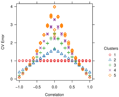
Figure 1: Cross-validation error on $10$ replicates, with the number of clusters $k$ ranging from $1$ to $5$. Data is generated from two-dimensional multivariate normal distribution with correlation $\rho$. The Gabriel cross-validation criterion chooses the correct answer $k=1$ whenever $|\rho|<0.5$; the criterion chooses $k\geq 2$ clusters whenever $|\rho|>0.5$.

Intuitively, when the correlation is high, the response feature, $Y$, looks similar to the predictor feature, $X$. Prediction error on $X$ always decreases with larger $k$. Thus, when the correlation is high, the prediction error for $Y$ will also decrease with larger $k$. This explains why cross-validation breaks down in the presence of strong correlation.

In Appendix B, using similar techniques to those used to prove Proposition 2, we derive an analogous result for correlated Gaussian noise in more than two dimensions. A similar phenomenon holds: the Gabriel cross-validation method fails when the first principal component of the $Y$ variables is strongly correlated with a linear combination of the $X$ variables.

Proposition 2 tells us that Gabriel cross-validation fails when there is strong correlation between the variables. To get around this, in practice we will transform the data to reduce correlation before performing cross-validation. We detail this approach in Section 5.

4.2 Two clusters in two dimensions

We will now analyze a simple two-cluster setting, and derive conditions for Gabriel cross-validation to correctly prefer $k=2$ clusters to $k=1$. The main assumption of the proposition is that the cluster centers are not too close. The precise definition of “too close” is stated in terms of $\Phi(\cdot)$ and $\varphi(\cdot)$, the standard normal cumulative distribution function and density, respectively. The inequality is hard to interpret directly, but we show the boundary between “too close” and “well separated” in Fig. 2, after the proof of the proposition.

Proposition 3.

Suppose that $\{(X_{i},Y_{i})\}_{i=1}^{n+m}$ is data from a single fold of Gabriel cross-validation, where each $(X,Y)$ pair in $\mathbb{R}^{2}$ is an independent draw from an equiprobable mixture of two multivariate normal distributions with identity covariance. Suppose that the first mixture component has mean $\mu=(\mu^{X},\mu^{Y})$ and the second has mean $-\mu=(-\mu^{X},-\mu^{Y})$, where $\mu^{X}\geq 0$ and $\mu^{Y}\geq 0$. If the cluster centers are well separated, specifically such that $2\varphi(\mu^{Y})+\mu^{Y}+2\mu^{Y}\Phi(\mu^{Y})<4\mu^{Y}\Phi(\mu^{X}),$ then $\operatorname{CV}(2)<\operatorname{CV}(1)$ with probability tending to one as $m$ and $n$ increase.

Proof.

There are two clusters: observations from cluster $1$ are distributed as $\mathcal{N}(\mu,I)$ and observations from cluster $2$ are distributed as $\mathcal{N}(-\mu,I)$ where $\mu=(\mu^{X},\mu^{Y})$. Without loss of generality, $\mu^{X}\geq 0$ and $\mu^{Y}\geq 0$. Let $G_{i}$ be the true cluster of observation $i$ where, by assumption,

$$\Pr(G_{i}=1)=\Pr(G_{i}=2)=1/2.$$

After applying $k$-means to $\{Y_{i}\}_{i=1}^{n}$ with $k=2$, if $n$ is large enough, then the estimated cluster means $\bar{\mu}^{Y}_{1}$ and $\bar{\mu}^{Y}_{2}$ will be close to $\operatorname{E}(Y\mid Y>0)$ and $\operatorname{E}(Y\mid Y<0)$, with errors of size $O_{p}(n^{-1/2})$. To compute these quantities, let $(X_{1},Y_{1})\sim\mathcal{N}(\mu,I)$ and $(X_{2},Y_{2})\sim\mathcal{N}(-\mu,I)$ be draws from the mixture components, and let $(X,Y)$ be defined such that $\Pr(X=X_{1},Y=Y_{1})=\Pr(X=X_{2},Y=Y_{2})=1/2$. Then,

$$\operatorname{E}(Y\mid Y>0) =\operatorname{E}(Y_{1}\mid Y_{1}>0)\cdot\Pr(Y=Y_{1}\mid Y>0)+\operatorname{E}(Y_{2}\mid Y_{2}>0)\cdot\Pr(Y=Y_{2}\mid Y>0)$$

$$=\{\mu^{Y}+\varphi(\mu^{Y})/\Phi(\mu^{Y})\}\cdot\Phi(\mu^{Y})+[-\mu^{Y}+\varphi(\mu^{Y})/\{1-\Phi(\mu^{Y})\}]\cdot\{1-\Phi(\mu^{Y})\}$$

$$=2\varphi(\mu^{Y})+2\mu^{Y}\Phi(\mu^{Y})-\mu^{Y}.$$

In the second line, we have used Lemma 3 from Appendix C to compute the conditional expectations; $\varphi()$ and $\Phi()$ are the standard normal density and cumulative distribution function, respectively. By symmetry,

$$\operatorname{E}(Y\mid Y<0) =-\operatorname{E}(Y\mid Y>0).$$

The classification rule learned from the training data $\{(X_{i},\hat{G}^{Y}_{i})\}_{i=1}^{n}$ will have its decision boundary at $0+O_{p}(n^{-1/2})$; that is, in the limit, observations will get classified as coming from cluster 1 when $X>0$. Set $a=\operatorname{E}(Y\mid Y>0)$. Up to terms of order $O_{p}(n^{-1/2})$, the cross-validation error from a single observation is distributed as

$$(Y-a)^{2}1\{X>0\}+(Y+a)^{2}1\{X<0\}.$$

Using the fact that conditional on the mixture component, the $X$ and $Y$ coordinates are independent, we can compute the expectation of the first summand as

$$\operatorname{E}[(Y-a)^{2}1\{X>0\}] =(1/2)\operatorname{E}[(Y_{1}-a)^{2}]\Pr(X_{1}>0)+(1/2)\operatorname{E}[(Y_{2}-a)^{2}]\Pr(X_{2}>0)$$

$$=(1/2)\Phi(\mu^{X})\operatorname{E}(Y_{1}-a)^{2}+(1/2)\{1-\Phi(\mu^{X})\}\operatorname{E}(Y_{2}-a)^{2}$$

$$=(1/2)[1+\Phi(\mu^{X})(\mu^{Y}-a)^{2}+\{1-\Phi(\mu^{X})\}(-\mu^{Y}-a)^{2}].$$

By a similar calculation, the expectation of the second summand is

$$\operatorname{E}[(Y+a)^{2}1\{X<0\}]=(1/2)[1+\{1-\Phi(\mu^{X})\}(\mu^{Y}+a)^{2}+\Phi(\mu^{X})(-\mu^{Y}+a)^{2}].$$

Adding the two terms, we get that the expected cross-validation error from a single observation is

$$1+\Phi(\mu^{X})(\mu^{Y}-a)^{2}+\{1-\Phi(\mu^{X})\}(\mu^{Y}+a)^{2}=1+(\mu^{Y})^{2}+a\,\{a+2\mu^{Y}-4\mu^{Y}\Phi(\mu^{X})\}.$$

Thus, the $k=2$ cross-validation error on the test set is

$$\operatorname{CV}(2) =\frac{1}{m}\sum_{i=n+1}^{n+m}\|(Y_{i}-\bar{\mu}^{Y}_{1})1\{\hat{G}^{X}_{i}=1\}\|^{2}+\|(Y_{i}-\bar{\mu}^{Y}_{2})1\{\hat{G}^{X}_{i}=2\}\|^{2}$$

$$=1+(\mu^{Y})^{2}+a\,\{a+2\mu^{Y}-4\mu^{Y}\Phi(\mu^{X})\}+O_{p}(n^{-1/2})+O_{p}(m^{-1/2}).$$

When $k=1$, the $k$-means centroid is equal to the sample mean $\bar{Y}_{n}=(1/n)\sum_{i=1}^{n}Y_{i}$, approximately equal to $\operatorname{E}(Y)=0$, with error of size $O_{p}(n^{-1/2})$. The cross-validation error is

$$\operatorname{CV}(1)=\frac{1}{m}\sum_{i=n+1}^{n+m}\|Y_{i}-\bar{Y}_{n}\|^{2}=1+(\mu^{Y})^{2}+O_{p}(m^{-1/2})+O_{p}(n^{-1/2}).$$

Thus, if $a+2\mu^{Y}-4\mu^{Y}\Phi(\mu^{X})<0$, then $\operatorname{CV}(2)<\operatorname{CV}(1)$ with probability tending to one as $m$ and $n$ increase. Substituting the expression for $\operatorname{E}(Y\mid Y>0)$ in place of $a$, the inequality holds precisely when $2\varphi(\mu^{Y})+\mu^{Y}+2\mu^{Y}\Phi(\mu^{Y})<4\mu^{Y}\Phi(\mu^{X}).$ ∎

We confirm the result of Proposition 3 with a simulation. We perform $10$ replicates for each $(\mu^{X},\mu^{Y})$ pair, sweeping over a two-dimensional grid of values in the domain $[0,3]\times[0,3]$, with step size $0.1$ in each dimension. In each replicate, we generate $N=20000$ observations from an equiprobably mixture of multivariate normal distributions with identity covariance, with one component having mean $(\mu^{X},\mu^{Y})$ and the other component having mean $(-\mu^{X},-\mu^{Y})$. We perform a single $2\times 2$ fold of Gabriel cross-validation and report the number of times (out of $10$ replicates) where $k=2$ is selected by the algorithm instead of $k=1$. Figure 2 shows the frequency with which $k=2$ is selected by the algorithm for each $(\mu^{X},\mu^{Y})$ pair. Darker (red) colors indicate higher numbers (close to $10$), situations where $k=2$ is selected more often than $k=1$. Ligher (blue) colors indicate that $k=1$ is preferred. We can see the simulation result perfectly align with the theoretical curve (the black line), which separates the $k=2$ zone from the $k=1$ zone.

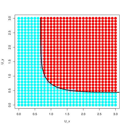
Figure 2: Number of times $k=2$ is selected out of $10$ replicates for each pair of $(\mu^{X},\mu^{Y})$. The heat map shows the frequency $k=2$ is selected by the algorithm, with light (blue) means $k=1$ is preferred to $k=2$, and dark (red) indicates $k=2$ is preferred to $k=1$. The black line is the theoretical boundary determined from Proposition 3.

5 Adjusting for correlation

Proposition 2 shows that when the correlation between dimensions is high, the Gabriel cross-validation method tends to overestimate the number of clusters, $k$. To mitigate this effect, we propose a two-stage estimation procedure that attempts to transform the data to minimize the correlation between features. In the first stage, we get a preliminary estimate for the number of clusters, $\hat{k}_{0}$, and we use this value to get an estimate of the noise covariance matrix. Then, in the second stage, we transform the data attempting to sphere the noise covariance, and re-estimate the number of clusters, getting a final estimate $\hat{k}$.

The details of the correlation correction procedure are as follow:

1. Apply the Gabriel cross-validation method on the original data $\mathfrak{X}$ to get a preliminary estimate of the number of clusters, $\hat{k}_{0}$.

2. Apply $k$-means to the full data set with observations $\mathfrak{X}_{1},\mathfrak{X}_{2},\dotsc,\mathfrak{X}_{N}$ using $k=\hat{k}_{0}$ clusters. For $i=1,\dotsc,N$, let $\hat{\mu}_{i}$ denote the assigned cluster mean for the $i$th observation.

3. Estimate the noise covariance matrix $\hat{\Sigma}$:

   $$\hat{\Sigma}=\frac{1}{N-\hat{k}_{0}}\sum^{N}_{i=1}(\mathfrak{X}_{i}-\hat{\mu}_{i})(\mathfrak{X}_{i}-\hat{\mu}_{i})^{T}.$$

4. Compute the eigendecomposition $\hat{\Sigma}=\Gamma\Lambda\Gamma^{T}$. Choose a random (Haar distributed) $P\times P$ orthogonal matrix $Q$. Rescale and rotate the original data matrix $\mathfrak{X}$ to get a transformed data matrix defined by

   $$\tilde{\mathfrak{X}}=\mathfrak{X}\Gamma\Lambda^{-1/2}Q.$$

5. Apply Gabriel cross-validation method to transformed data matrix $\tilde{\mathfrak{X}}$ to get a final estimate for the number of clusters, $\hat{k}$.

The noise covariance estimate assumes a shared covariance matrix for all $k$ clusters. Letting $G_{i}$ denote the cluster membership of the $i$th observation, and letting $\mu(g)$ denote the mean of cluster $g$ for $g=1,\dotsc,k$, the model supposes that

$$\mathfrak{X}_{i}=\mu(G_{i})+\varepsilon_{i},$$

where $\varepsilon_{i}$ has mean zero and covariance matrix $\Sigma$, independent of $G_{i}$. If we knew $\Sigma$, then we could transform the observations as

$$\Sigma^{-1/2}\mathfrak{X}_{i} =\Sigma^{-1/2}\mu(G_{i})+\Sigma^{-1/2}\varepsilon_{i}$$

$$=\tilde{\mu}(G_{i})+\tilde{\varepsilon}_{i},$$

where $\tilde{\mu}=\Sigma^{-1/2}\mu$ and $\tilde{\varepsilon}_{i}=\Sigma^{-1/2}\varepsilon_{i}$. The transformed data has the same number of clusters, but has noise covariance $\operatorname*{cov}(\tilde{\varepsilon}_{i})=I$. The matrix product $\Gamma\Lambda^{-1/2}$ used in step 4 is an estimate of $\Sigma^{-1/2}$.

The transformation used in step 4 uses a random orthogonal matrix $Q$, which gets applied to the rows of $\mathfrak{X}$ after multiplying by the estimate of $\Sigma^{-1/2}$. We use this random orthogonal matrix for two reasons. First, it ensures that in expectation, each transformed cluster mean $Q\Lambda^{-1/2}\Gamma^{T}\mu(g)$ for $g=1,\dotsc,k$ is uniformly spread across all $P$ features. This ensures that the self-consistency conditions on the cluster centers enumerated in Proposition 1 are likely to hold. The second reason for multiplying by $Q$ is to spread any remaining correlation in the noise evenly (in expectation) across all dimensions. The latter effect follows since if $Z$ is a random vector with covariance matrix $\Theta$, then $QZ$ has covariance matrix $Q\Theta Q^{T}$, which has expectation $E(Q\Theta Q^{T})=\operatorname*{tr}(\Theta)I$.

Our correlation correction is not backed by a rigorous theoretical justification. However, the simulations and empirical validation in Sections 6 and 7 demonstrate the effectiveness of our ad-hoc adjustment procedure.

6 Performance in simulations

6.1 Overview

In this section, we perform a set of simulations to evaluate the performance of our proposed method and the associated correlation correction described in Section 5. We compare our method with a basket of competing methods including the Gap statistic (Tibshirani et al.,, 2001), Gaussian mixture model-based clustering (Fraley and Raftery,, 2002), the CH-index (Caliński and Harabasz,, 1974), Hartigan’s statistic (Hartigan,, 1975), the Jump method (Sugar and James,, 2003), Prediction strength (Tibshirani and Walther,, 2005), and Bootstrap stability (Fang and Wang,, 2012). We use the default parameter settings for all competing methods. For Gabriel cross-validation, we perform $2$-fold cross-validation on the columns ($p=q$) and $5$-fold cross-validation on the rows ($m=n/4$). We also compare with Wold cross-validation, which we describe in Appendix D.

In all simulation settings, we randomly generate cluster centers by drawing from a multivariate normal distribution with covariance matrix $\tau I$, conditional on the cluster centers being well-separated (if the distance between any two cluster centers is less than $1$, then we re-draw a new set of cluster centers). We choose $\tau$ to make the probability the cluster centers being well-separated on the first draw to be equal to approximately 50%. Many of our simulation settings are chosen to mimic the settings used by Tibshirani et al., (2001).

For each setting, we perform $100$ replicates. We report the number of times that each method finds the correct number $k$ of clusters. We also report 95% confidence intervals for the proportions, using Wilson’s method (Wilson,, 1927). The simulations demonstrate that overall, the proposed Gabriel cross-validation method and its correlation-corrected version compare well with the competing methods, and they are robust to variance heterogeneity, high dimensional data, and heavy-tail data.

6.2 Setting 1: Correlation between dimensions

We generate six clusters in $10$ dimensions. Each cluster has $100$ or $50$ multivariate normal observations with common covariance matrix $\Sigma$ which has compound symmetric structure with $1$ in diagonal and $\rho$ off diagonal. $\rho$ takes value in $\{0,0.1,...,0.9\}$.

We can see that high correlation between dimensions causes problem for most existing methods, including Gabriel cross-validation method without the correlation correction. The only two methods that work well in the presence of high correlation are the Gaussian model-based BIC method (Fraley and Raftery,, 2002) and the correlation-corrected Gabriel method.

6.3 Setting 2: Noise dimensions

We generate three clusters in $6$ dimensions. Each cluster has $1000$ or $500$ multivariate normal observations with identity covariance matrix. We add $r$ dimensions of noise to the data, randomly generated from a uniform distribution on $[0,1]$. The noise dimension $r$ takes values in $\{0,6,...,54\}$.

Most methods are relatively insensitive to adding more noise dimensions; the one exception to this is the Jump method, which deteriorates significantly in the presence of extra noise dimensions.

6.4 Setting 3: High dimension

We generate eight clusters in $P$ dimensions, with $P$ taking values in $\{10,20,...,100\}$. Each cluster has $100$ or $50$ multivariate normal observations with identity covariance matrix.

Some methods, like Jump and Gap, are insensitive to higher dimensions while other methods deteriorate quickly with increasing dimension, most notably the Gaussian model-based BIC method. Gabriel cross-validation and its correlation-corrected version tend to work better in higher dimensions.

6.5 Setting 4: Variance heterogeneity

We generate three clusters in $20$ dimensions. Each cluster has $60$ observations. Observations are generated from $\mathcal{N}\left(\mathbf{0},\sigma_{1}^{2}\mathbf{I}\right)$, $\mathcal{N}\left(\mathbf{0},\sigma_{2}^{2}\mathbf{I}\right)$ and $\mathcal{N}\left(\mathbf{0},\sigma_{3}^{2}\mathbf{I}\right)$ where $\sigma_{1}^{2}:\sigma_{2}^{2}:\sigma_{3}^{2}=1:\frac{1+R}{2}:R$. The maximum ratio $R$ takes values in $\{1,5,10,...,45\}$

This setting demonstrates that most existing methods are sensitive to variance heterogeneity, most notably the Gap method and the model-based BIC method. The proposed Gabriel cross-validation method and its correlation-corrected version consistently perform well in estimating $k$ and they are insensitive to variance heterogeneity.

6.6 Setting 5: Heavy tail data

We generate five clusters in $15$ dimensions. Each cluster has $80$ observations. Observations have independent $t$ distributions in each dimension, with degrees of freedom $\nu$ taking values in $\{11,10,...,2\}$

This setting investigates performance in the presence of heavy-tailed data. When the degrees of freedom decreases, the tail becomes more flat and the Gaussian assumption becomes more inappropriate. For most methods, their performances are relatively stable until the tail gets very heavy. In the case where there are $2$ degrees of freedom, the Gap and Jump methods’ performances deteriorate considerably relative to the Gabriel method.

7 Empirical validation

To further validate our method, we applied it to three real world data sets with known clustering structure.

The first data set is congressional voting data consisting of voting records of the second session of the $98$th United States Congress, (Schlimmer,, 1987). This data set includes votes for legislators on the $P=16$ key votes. For each vote, each legislator either votes positively (“yea”) or negatively (“nay”). We removed legislators with missing votes. This results in $N=232$ remaining records, with $124$ democrat and $108$ republican. There are $k=2$ clusters of legislators, corresponding to political party.

The second benchmark is the Mangasarian et al., (1990) Wisconsin breast cancer data set. After excluding the records with missing data, this data set consists records of $N=683$ patients, each with measurements of $P=9$ attributes of their biopsy specimens. It is known that there are $k=2$ groups of patients: $444$ patients with benign specimens and $239$ patients with malignant specimens. There is some disagreement as to what the “true” value of $k$ should be for this data set; Fujita et al., (2014) have argued that the malign group is heterogeneous, and should be split into two smaller clusters, yielding $k=3$.

The third data set is gene expression data of $k=5$ types of brain tumors from Pomeroy et al., (2002), which contains $N=42$ observations including $10$ medulloblastomas, $10$ malignant gliomas, $10$ atypical teratoid/rhabdoid tumors, $8$ primitive neuroectodermal tumours and $4$ normal cerebella. After preprocessing and feature selection, there are $P=1379$ variables, corresponding to log activation levels for 1379 genes.

Table 1: Number of clusters selected on benchmark datasets

	Dataset
Method	Congress Voting	Breast Cancer	Brain Tumours
Gabriel	$2$	$3$	$5$
Gabriel (corr. correct)	$2$	$2$	$5$
Wold	$2$	$3$	$4$
Gap	$8$	$10$	$10$
BIC	$2$	$5$	$2$
CH	$2$	$2$	$2$
Hartigan	$3$	$3$	$4$
Jump	$10$	$9$	$1$
PS	$2$	$2$	$1$
Stab.	$2$	$2$	$7$
Ground Truth	$2$	$2$ or $3$	$5$

We applied the Gabriel cross-validation method, the correlation-corrected version, and the competing methods described in Section 6 to each of the three benchmark datasets. In each dataset, we allowed the number of clusters, $k$, to range from $1$ to $10$. Table 1 displays the results. Both versions of the Gabriel method perform well on all three benchmark datasets. In fact, Gabriel cross-validation is the only method that correctly identifies the number of clusters in all three benchmark datasets.

8 Application to yeast cell cycle data

8.1 Motivation

Now that we have established that Gabriel cross-validation can effectively estimate the number of clusters, we apply our method to a yeast cell cycle dataset. This dataset was collected by Cho et al., (1998) to study the cell cycle of budding yeast Saccharomyces cerevisiae. Other authors, including Tavazoie et al., (1999) and Dortet-Bernadet and Wicker, (2008) have used $k$-means and related methods to cluster the genes in the dataset, with $k$ approximately equal to 30. In both of these analyses, the authors discard the majority of their clusters as uninterpretable or noise, focusing instead on a small number of clusters. In contrast to these previous analyses, Gabriel cross-validation finds a small number, $k=5$ clusters, all of which are interpretable.

8.2 Data collection and preprocessing

To obtain the raw data, Cho et al., (1998) first synchronized a collection of CDC28 yeast cells by raising their temperature to $37^{\circ}$C in the late G1 cell cycle phase, then they reinitiated the cell cycle by switching them to a cooler environment ($25^{\circ}$C). The authors collected data at $17$ time points spaced evenly at $10$-minute intervals, covering almost $2$ complete cell cycles. At each of the $17$ time points, they used oligonucleotide microarrays to measure $6220$ gene expression profiles.

Tavazoie et al., (1999) preprocessed the raw data in an attempt to normalize the gene responses and remove noise. They reduced the original $6220$ gene expression profiles to just the $2945$ genes with the highest variances. Then, they removed the time points at $90$ and $100$ minutes, because they deemed the measurements at these time points to be unreliable. Finally, they centered and scaled the genes by subtracting the means and dividing by the standard deviations, as computed from the remaining $15$ time points. After the preprocessing, the data matrix $\mathfrak{X}$ has $N=2945$ genes and $P=15$ time points.

We obtained the preprocessed data and the Tavazoie et al., (1999) cluster analysis from http://arep.med.harvard.edu/network_discovery/.

8.3 Clustering

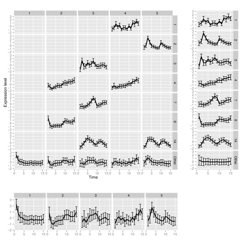
Figure 3: Yeast data set mean expression profiles. The $5$ clusters found by the Gabriel method are on the bottom; Clusters profiled in Tavazoie et al., (1999) are on the right.

Following Tavazoie et al., (1999) and Dortet-Bernadet and Wicker, (2008), we treat the $N=2945$ gene expression profiles as draws from a mixture distribution, and we perform $k$-means clustering to segment the genes according to their expression profiles across the $P=15$ time points. Both the original and the correlation-corrected version of Gabriel cross-validation find $k=5$ clusters.

The lower-left panel of Figure 3 shows the average expression level for each cluster across the 15 time points, with error bars showing standard deviations. Cluster $1$ has decreasing expression level with time. The mean gene expression level in Cluster $2$ decreases at the beginning and then increases. Cluster $3$ is a periodic cluster where one can see two periods corresponding to the two cell cycles. Cluster $4$ has increasing expression level with time. Cluster $5$ is another periodic cluster.

8.4 Enrichment analysis

To further validate our clusters, we follow Tavazoie et al., (1999), performing an enrichment analysis to discover which functional gene groups are significantly over-represented in each cluster. In the Saccharomyces Genome Database, each gene is mapped to a set of Gene Ontology categories. We focus on the $103$ biological process categories.

Table 2: Biological process enrichment within gene clusters

Cluster	Cluster Size	Process Category (In Cluster/Total Genes)	$p$-value
$1$	$550$	response to oxidative stress ($24/55$)	$1.5\times 10^{-5}$
		response to chemical ($64/213$)	$2.2\times 10^{-5}$
$2$	$590$	mitochondrion organization ($79/159$)	$1.1\times 10^{-16}$
		mitochondrial translation ($28/51$)	$2.9\times 10^{-8}$
		generation of precursor metabolites and energy ($37/80$)	$7.3\times 10^{-8}$
$3$	$654$	transcription from RNA polymerase II promoter ($75/214$)	$5.5\times 10^{-6}$
		mRNA processing ($30/67$)	$2.7\times 10^{-5}$
		mitotic cell cycle ($63/183$)	$6.2\times 10^{-5}$
$4$	$634$	cytoplasmic translation ($105/134$)	$3.3\times 10^{-47}$
		ribosomal subunit biogenesis ($73/138$)	$7.7\times 10^{-17}$
		rRNA processing ($61/131$)	$5.7\times 10^{-11}$
		ribosome assembly ($21/36$)	$1.5\times 10^{-6}$
$5$	$517$	chromosome segregation ($53/106$)	$6.0\times 10^{-15}$
		cellular response to DNA damage stimulus ($71/172$)	$3.6\times 10^{-14}$
		DNA repair ($64/147$)	$3.7\times 10^{-14}$
		DNA replication ($42/78$)	$1.8\times 10^{-13}$
		mitotic cell cycle ($70/183$)	$4.8\times 10^{-12}$

For each category and each cluster, we compute a $p$-value for the null hypothesis that genes from the category are distributed across all clusters without any bias towards the particular cluster in question. Under the null hypothesis, the number of genes from the category that end up in the cluster is distributed as a hypergeometric random variable. For each cluster, we compute $p$-values for all $103$ biological process categories, and we report those that are significantly enrigched in Table 2. Using a Bonferroni correction to control the family-wise error rate at level 5%, we only report $p$-values that are less than $0.05/103=4.8\times 10^{-4}$.

From Table 2, we can see that Cluster 1 is enriched with genes that somatize cell stress, such as oxidative heat-induce proteins. Cluster 2 contains genes that govern mitochondrial translation and mitochondrion organization. Cluster 3, the first period cluster, contains cell cycle genes related to budding and cell polarity, along with genes that govern RNA processing and transcription. Cluster 4 contains genes related to cytoplasmic translation and genes encoding ribosomes. Cluster 5, the second periodic cluster, contains genes that participate cell-cycle processes, along with DNA replication and DNA repair.

8.5 Comparison with Tavazoie clusters

In the Tavazoie et al., (1999) analysis, those authors performed $k$-means clustering with $k=30$; they found 23 of the clusters to be uninterpretable, and they found 7 clusters to be meaningful. To compare our clusters with the Tavazoie et al. clusters, we prepared a confusion matrix comparing our clusters with the 7 interpretable Tavazoie clusters in Table 3. Entry $(i,j)$ of the confusion matrix gives the number of genes in Tavazoie’s Cluster $i$ and our Cluster $j$.

Table 3: Confusion matrix comparing the 5 clusters found by Gabriel cross-validation to the 7 interpretable clusters found by the Tavazoie et al., (1999) analysis

	Cluster 1	Cluster 2	Cluster 3	Cluster 4	Cluster 5	Total
Cluster 1	0	0	1	161	2	164
Cluster 2	1	0	0	0	185	186
Cluster 3	0	0	91	11	2	104
Cluster 4	0	102	2	66	0	170
Cluster 7	1	10	83	7	0	101
Cluster 8	3	145	0	0	0	148
Cluster 14	0	1	29	6	38	74
Other	545	332	448	383	290	1998
Total	550	590	654	634	517	2945

Figure 3 provides a more in-depth comparison with the Tavazoie clusters, using a graphical confusion matrix. The plot in cell $(i,j)$ of the upper left part of this figure gives the mean expression level for genes in the intersection of Tavazoie’s Cluster $i$ and our Cluster $j$; the plots in the margins give the mean expression levels for Tavazoie’s clusters (top right) and our clusters (bottom left). In Figure 3, we only include a plot for cell $(i,j)$ if the number of genes in that cell is greater than $20$.

Our Cluster 1 mainly consists of genes that Tavazoie et al. found to be in uninterpretable clusters. Our Cluster 2 contains high concentrations of Tavazoie’s Clusters 4 and 8. Our first periodic cluster, Cluster 3, contains high concentrations of Tavazoie’s Clulsters 3, 7, and 14; this is notable, because Tavazoie et al. highlighted their Clusters 7 and 14 as being periodic. Our Cluster 4 contains almost all of Tavazoie’s Cluster 1, along with part of Tavazoie’s Cluster 4. Finally, our second periodic cluster, Cluster 5, contains almost all of Tavazoie’s Cluster 2, along with part of Tavazoie’s Cluster 14; this, again, is notable, because Tavazoie et al. highlited these clusters as being periodic.

For the clusters that Tavazoie et al. were able to characterize, our analysis broadly agrees with the earlier clustering. The major difference between our analysis and that of Tavazoie et al., (1999) is that we are able to identify meaningful groups of genes with a much smaller value of $k$ ($k=5$ instead of $k=30$), and we are able to interpret all of the clusters found by our analysis.

9 Discussion

In this paper, we proposed a new approach to estimate the number of clusters to be used in $k$-means clustering. The intuition behind our proposed method is to transform the unsupervised learning problem into a supervised learning problem via a form of Gabriel cross validation. We proved that our method is self-consistent, and we analyzed its behavior in some special cases of Gaussian mixture models. Using simulations and real data examples, we demonstrated that our method has good performance, competitive with existing approaches. The simulations and empirical benchmarks demonstrate the advantages of our method. In the yeast cell cycle application, our method was able to identify meaningful gene groups with a small number of clusters.

There are many other clustering algorithms that get used in practice besides $k$-means. We suspect that it should be possible to apply our method in the context of a spectral clustering procedure, after transforming by the eigenvectors of the Laplacian matrix. For other clustering schemes, including versions of hierarchical clustering, we are less certain about the viability of Gabriel cross-validation. It is an open question as to whether Gabriel cross-validation can be extended to other clustering methods, and whether such extensions will perform well in practice.

For $k$-means clustering, Gabriel cross-validation is competitive with other model selection methods, especially in the presence of high-dimensional, heterogeneous, or heavy-tailed data.

Appendix A Clustering scree plot examples

The top row of Figure 4 displays an example where the elbow in $W_{k}$ corresponds to the true number $k=4$ of mixture components in the data-generating mechanism. The elbow approach is simple and often performs well, but it requires subjective judgment as to where the elbow is located, and, as the bottom row of Figure 4 demonstrates, the approach can easily fail.

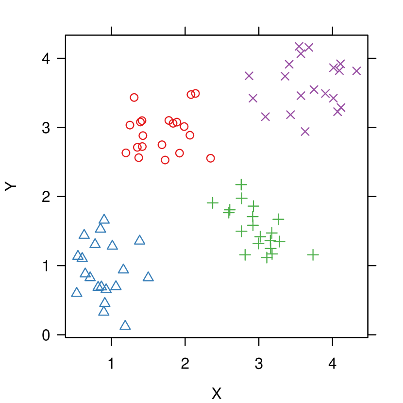
Figure 4: Left panels show the $(X,Y)$ data points; right panels show the corresponding values of the within-cluster sum of squares $W_{k}$ plotted against the number of clusters, $k$.

Appendix B Analysis of Gabriel method: Single cluster in more than two dimensions

Proposition 4.

Suppose that $\{(X_{i},Y_{i})\}_{i=1}^{n+m}$ is data from a single fold of Gabriel cross-validation, where each $(X,Y)$ pair in $\mathbb{R}^{p+q}$ is an independent draw from a mean-zero multivariate normal distribution with covariance matrix $\Sigma_{XY}=\left(\begin{smallmatrix}\Sigma_{XX}&\Sigma_{XY}\\ \Sigma_{YX}&\Sigma_{YY}\end{smallmatrix}\right)$, with $\Sigma_{YY}$ has leading eigenvalue $\lambda_{1}$ and corresponding eigenvector $u_{1}$. In this case, the data are drawn from a single cluster; the true number of clusters is $1$. If $\frac{\sqrt{\lambda_{1}}}{2}>\frac{u^{T}_{1}\Sigma_{YX}\Sigma_{XY}u_{1}}{\sqrt{u^{T}_{1}\Sigma_{YX}\Sigma_{XX}\Sigma_{XY}u_{1}}}$, then $\operatorname{CV}(1)<\operatorname{CV}(2)$ with probability tending to one as $m$ and $n$ increase.

Proof.

Let $X$ and $Y$ be jointly multivariate normal distributed with mean $\mathbf{0}$ and covariance matrix $\Sigma_{XY}$, i.e.

$$(X,Y)\sim\mathcal{N}\left(\mathbf{0},\Sigma_{XY}\right)$$

where $\Sigma_{XY}=\begin{bmatrix}\Sigma_{XX}&\Sigma_{XY}\\ \Sigma_{YX}&\Sigma_{YY}\end{bmatrix}$.

Let $\Sigma_{YY}=U\Lambda U^{T}$ be the eigendecomposition of $\Sigma_{YY}$, with leading eigenvalue $\lambda_{1}$ and corresponding eigenvector $u_{1}$. Then the centroid of $k$-means applying on $(y_{1},..,y_{n})$ is on the first principal component of $Y$,

$$E(u^{T}_{1}Y|u^{T}_{1}Y>0)=\bar{\mu}^{Y}_{1}=\sqrt{2\lambda_{1}/\pi}u_{1}$$

and

$$E(u^{T}_{1}Y|u^{T}_{1}Y<0)=\bar{\mu}^{Y}_{2}=-\sqrt{2\lambda_{1}/\pi}u_{1}$$

where $u^{T}_{1}Y\sim\mathcal{N}(0,\lambda_{1})$.

To compute $\bar{\mu}^{X}_{1}=E(X|u^{T}_{1}Y>0)$, we need to know the conditional distribution $X|u^{T}_{1}Y$. Since $(X,Y)$ has multivariate normal distribution, $(X,u^{T}_{1}Y)$ also has a multivariate normal distribution with mean $\mathbf{0}$ and covariance matrix

$$\Sigma_{X,u^{T}_{1}Y}=\begin{bmatrix}\Sigma_{XX}&\Sigma_{XY}u_{1}\\ u^{T}_{1}\Sigma_{YX}&\lambda_{1}\end{bmatrix}$$

The conditional distribution $X|u^{T}_{1}Y$ is hence normal with mean

$$\mu_{X|u^{T}_{1}Y}=\Sigma_{XY}u_{1}\lambda^{-1}_{1}u^{T}_{1}Y$$

Therefore,

$$\bar{\mu}^{X}_{1} =E(X\mid u^{T}_{1}Y>0)$$

$$=E\left(E[X\mid u^{T}_{1}Y]\mid u^{T}_{1}Y>0\right)$$

$$=E\left(\Sigma_{XY}u_{1}\lambda^{-1}_{1}u^{T}_{1}Y\mid u^{T}_{1}Y>0\right)$$

$$=\lambda^{-1}_{1}\Sigma_{XY}u_{1}E(u^{T}_{1}Y\mid u^{T}_{1}Y>0)$$

$$=\lambda^{-1}_{1}\Sigma_{XY}u_{1}\sqrt{2\lambda_{1}/\pi}$$

$$=\sqrt{2/(\lambda_{1}\pi)}\Sigma_{XY}u_{1}$$

Similar calculation yields $\bar{\mu}^{X}_{2}=-\sqrt{2/(\lambda_{1}\pi)}\Sigma_{XY}u_{1}$. The decision rule to classify any observed value of $X$ to $\bar{\mu}^{X}_{1}$ is therefore

$$(\bar{\mu}^{X}_{1})^{T}X>0\hskip 14.45377pt\text{or}\hskip 14.45377ptu^{T}_{1}\Sigma_{YX}X>0$$

Since $u^{T}_{1}\Sigma_{YX}X$ is a linear combination of $X$, it also has normal distribution

$$\mathcal{N}\left(0,u^{T}_{1}\Sigma_{YX}\Sigma_{XX}\Sigma_{XY}u_{1}\right)$$

And $(Y,u^{T}_{1}\Sigma_{YX}X)$ also have multivariate normal distribution with mean $\mathbf{0}$ and covariance matrix

$$\begin{bmatrix}\Sigma_{YY}&\Sigma_{YX}\Sigma_{XY}u_{1}\\ u^{T}_{1}\Sigma_{YX}\Sigma_{XY}&u^{T}_{1}\Sigma_{YX}\Sigma_{XX}\Sigma_{XY}u_{1}\end{bmatrix}$$

The conditional distribution of $Y|u^{T}_{1}\Sigma_{YX}X$ is also multivariate normal with mean

$$\mu_{Y|u^{T}_{1}\Sigma_{YX}X}=\Sigma_{YX}\Sigma_{XY}u_{1}(u^{T}_{1}\Sigma_{YX}\Sigma_{XX}\Sigma_{XY}u_{1})^{-1}u^{T}_{1}\Sigma_{YX}X$$

The $Y$ center for $u^{T}_{1}\Sigma_{YX}X>0$ is

$$\hat{\mu}^{Y}_{1} =E(Y|u^{T}_{1}\Sigma_{YX}X>0)$$

$$=\Sigma_{YX}\Sigma_{XY}u_{1}(u^{T}_{1}\Sigma_{YX}\Sigma_{XX}\Sigma_{XY}u_{1})^{-1}E(u^{T}_{1}\Sigma_{YX}X\mid u^{T}_{1}\Sigma_{YX}X>0)$$

Note that $u^{T}_{1}\Sigma_{YX}X$ has normal distribution $\mathcal{N}\left(0,u^{T}_{1}\Sigma_{YX}\Sigma_{XX}\Sigma_{XY}u_{1}\right)$, so

$$E(u^{T}_{1}\Sigma_{YX}X\mid u^{T}_{1}\Sigma_{YX}X>0)=\sqrt{2/\pi}\cdot\sqrt{u^{T}_{1}\Sigma_{YX}\Sigma_{XX}\Sigma_{XY}u_{1}}$$

Therefore, we have the $Y$ center for $u^{T}_{1}\Sigma_{YX}X>0$ be

$$\hat{\mu}^{Y}_{1} =\sqrt{2/\pi}\cdot\sqrt{u^{T}_{1}\Sigma_{YX}\Sigma_{XX}\Sigma_{XY}u_{1}}\hskip 7.22743pt\Sigma_{YX}\Sigma_{XY}u_{1}(u^{T}_{1}\Sigma_{YX}\Sigma_{XX}\Sigma_{XY}u_{1})^{-1}$$

$$=\frac{\sqrt{2/\pi}}{\sqrt{u^{T}_{1}\Sigma_{YX}\Sigma_{XX}\Sigma_{XY}u_{1}}}\Sigma_{YX}\Sigma_{XY}u_{1}$$

Recall that $\bar{\mu}^{Y}_{1}=\sqrt{2\lambda_{1}/\pi}u_{1}$, to judge if $\operatorname{CV}(2)>\operatorname{CV}(1)$, one only need to compare the distance between $\hat{\mu}^{Y}_{1}$ and $\bar{\mu}^{Y}_{1}$ with distance between $\hat{\mu}^{Y}_{1}$ and grand mean $0$. By the variance and bias decomposition of prediction MSE, when variance is the same, only bias influences the MSE.

After some linear algebra manipulation, we get $\|\hat{\mu}^{Y}_{1}-\bar{\mu}^{Y}_{1}\|^{2}>\|\hat{\mu}^{Y}_{1}\|^{2}$ or $\operatorname{CV}(2)>\operatorname{CV}(1)$ if and only if

$$\frac{\sqrt{\lambda_{1}}}{2}>\frac{u^{T}_{1}\Sigma_{YX}\Sigma_{XY}u_{1}}{\sqrt{u^{T}_{1}\Sigma_{YX}\Sigma_{XX}\Sigma_{XY}u_{1}}}$$

∎

Appendix C Technical Lemmas

Lemma 3.

If $Z$ is a standard normal random variable, then

$$\operatorname{E}(Z\mid a<Z<b)=-\frac{\varphi(b)-\varphi(a)}{\Phi(b)-\Phi(a)}$$

and

$$\operatorname{E}\{(Z-\delta)^{2}\mid a<Z<b\}=\delta^{2}+1-\frac{(b-2\delta)\varphi(b)-(a-2\delta)\varphi(a)}{\Phi(b)-\Phi(a)}$$

for all constants $a$, $b$, and $\delta$, where $\varphi(z)$ and $\Phi(z)$ are the standard normal probability density and cumulative distribution functions. These expressions are valid for $a=-\infty$ or $b=\infty$ by taking limits.

Proof.

We will derive the expression for the second moment. Integrate to get

$$\operatorname{E}[(Z-\delta)^{2}1\{Z<b\}] =\int_{-\infty}^{b}(z-\delta)^{2}\varphi(z)\,dz$$

$$=(\delta^{2}+1)\Phi(b)-(b-2\delta)\varphi(b).$$

Now,

$$\operatorname{E}\{(Z-\delta)^{2}\mid a<Z<b\}=\frac{\operatorname{E}[(Z-\delta)^{2}1\{Z<b\}]-\operatorname{E}[(Z-\delta)^{2}1\{Z<a\}]}{\Phi(b)-\Phi(a)}.$$

∎

Lemma 3 has some important special cases:

$$\operatorname{E}\{Z\mid Z>0\} =2\varphi(0)=\sqrt{2/\pi},$$

$$\operatorname{E}\{(Z-\delta)^{2}\mid Z>0\} =\delta^{2}+1-4\delta\varphi(0),$$

$$\operatorname{E}\{(Z-\delta)^{2}\mid Z<0\} =\delta^{2}+1+4\delta\varphi(0).$$

Appendix D Wold cross-validation

In Wold cross-validation, we perform “speckled” hold-outs in each fold, leaving out a random subset of the entries of the data matrix $\mathfrak{X}\in\mathbb{R}^{N\times P}$. For each value of $k$ and each fold, we perform the following set of actions to get an estimate of cross-validation error, $\operatorname{CV}(k)$, which we average over all folds.

1. Randomly partition the set of indices $\{1,2,\dotsc,N\}\times\{1,2,\dotsc,P\}$ into a train set $S_{\text{train}}$ and a test set $S_{\text{test}}$.

2. Apply a $k$-means fitting procedure that can handle missing data to the training data $\{\mathfrak{X}_{i,j}:(i,j)\in S_{\text{train}}\}$. This gives a set of cluster means $\mu(1),\dotsc,\mu(k)\in\mathbb{R}^{P}$ and cluster labels for the rows, $G_{1},G_{2},\dotsc,G_{N}$.

3. Compute the cross-validation error as

   $$\operatorname{CV}(k)=\sum_{(i,j)\in S_{\text{test}}}\{\mathfrak{X}_{i,j}-\mu_{j}(G_{i})\}^{2},$$

   where $\mu_{j}(G_{i})$ denotes the $j$th component of $\mu(G_{i})$.

References

- Ben-Hur et al., (2001) Ben-Hur, A., Elisseeff, A., and Guyon, I. (2001). A stability based method for discovering structure in clustered data. In Pacific symposium on biocomputing, volume 7, pages 6–17.
- Caliński and Harabasz, (1974) Caliński, T. and Harabasz, J. (1974). A dendrite method for cluster analysis. Communications in Statistics-theory and Methods, 3(1):1–27.
- Chiang and Mirkin, (2010) Chiang, M. M.-T. and Mirkin, B. (2010). Intelligent choice of the number of clusters in k-means clustering: an experimental study with different cluster spreads. Journal of classification, 27(1):3–40.
- Cho et al., (1998) Cho, R. J., Campbell, M. J., Winzeler, E. A., Steinmetz, L., Conway, A., Wodicka, L., Wolfsberg, T. G., Gabrielian, A. E., Landsman, D., Lockhart, D. J., et al. (1998). A genome-wide transcriptional analysis of the mitotic cell cycle. Molecular cell, 2:65–73.
- Dortet-Bernadet and Wicker, (2008) Dortet-Bernadet, J.-L. and Wicker, N. (2008). Model-based clustering on the unit sphere with an illustration using gene expression profiles. Biostatistics, 9(1):66–80.
- Fang and Wang, (2012) Fang, Y. and Wang, J. (2012). Selection of the number of clusters via the bootstrap method. Computational Statistics & Data Analysis, 56(3):468–477.
- Fraley and Raftery, (2002) Fraley, C. and Raftery, A. E. (2002). Model-based clustering, discriminant analysis, and density estimation. Journal of the American Statistical Association, 97(458):611–631.
- Fujita et al., (2014) Fujita, A., Takahashi, D. Y., and Patriota, A. G. (2014). A non-parametric method to estimate the number of clusters. Computational Statistics & Data Analysis, 73:27–39.
- Gabriel, (2002) Gabriel, K. R. (2002). Le biplot–outil d’exploration de données multidimensionelles. Journal de la Société Francaise de Statistique, 143:5–55.
- Hartigan, (1975) Hartigan, J. A. (1975). Clustering Algorithms. Wiley.
- Hartigan and Wong, (1979) Hartigan, J. A. and Wong, M. A. (1979). Algorithm as 136: A k-means clustering algorithm. Journal of the Royal Statistical Society. Series C (Applied Statistics), 28:100–108.
- Hastie et al., (2009) Hastie, T., Tibshirani, R., and Friedman, J. (2009). The Elements of Statistical Learning: Data Mining, Inference, and Prediciton. Springer Series in Statistics. Springer, 2nd edition.
- Jain, (2010) Jain, A. K. (2010). Data clustering: 50 years beyond k-means. Pattern recognition letters, 31(8):651–666.
- Jain et al., (1999) Jain, A. K., Murty, M. N., and Flynn, P. J. (1999). Data clustering: a review. ACM computing surveys (CSUR), 31(3):264–323.
- Mangasarian et al., (1990) Mangasarian, O. L., Setiono, R., and Wolberg, W. (1990). Pattern recognition via linear programming: Theory and application to medical diagnosis. Large-scale numerical optimization, pages 22–31.
- Owen and Perry, (2009) Owen, A. B. and Perry, P. O. (2009). Bi-cross-validation of the svd and the nonnegative matrix factorization. Ann. Appl. Stat., 3(2):564–594.
- Pollard, (1981) Pollard, D. (1981). Strong consistency of -means clustering. Ann. Stat., 9(1):135–140.
- Pomeroy et al., (2002) Pomeroy, S. L., Tamayo, P., Gaasenbeek, M., Sturla, L. M., Angelo, M., McLaughlin, M. E., Kim, J. Y., Goumnerova, L. C., Black, P. M., Lau, C., et al. (2002). Prediction of central nervous system embryonal tumour outcome based on gene expression. Nature, 415(6870):436–442.
- Schlimmer, (1987) Schlimmer, J. C. (1987). Concept acquisition through representational adjustment. PhD thesis, Department of Information and Computer Science, University of California, Irvine.
- Sugar and James, (2003) Sugar, C. A. and James, G. M. (2003). Finding the number of clusters in a dataset. Journal of the American Statistical Association, 98(463).
- Tarpey and Flury, (1996) Tarpey, T. and Flury, B. (1996). Self-consistency: A fundamental concept in statistics. Statist. Sci., 11(3):229–243.
- Tavazoie et al., (1999) Tavazoie, S., Hughes, J. D., Campbell, M. J., Cho, R. J., and Church, G. M. (1999). Systematic determination of genetic network architecture. Nature genetics, 22:281–285.
- Tibshirani and Walther, (2005) Tibshirani, R. and Walther, G. (2005). Cluster validation by prediction strength. Journal of Computational and Graphical Statistics, 14(3):511–528.
- Tibshirani et al., (2001) Tibshirani, R., Walther, G., and Hastie, T. (2001). Estimating the number of clusters in a data set via the gap statistic. Journal of the Royal Statistical Society: Series B (Statistical Methodology), 63(2):411–423.
- Wang, (2010) Wang, J. (2010). Consistent selection of the number of clusters via crossvalidation. Biometrika, 97(4):893–904.
- Wilson, (1927) Wilson, E. B. (1927). Probable inference, the law of succession, and statistical inference. Journal of the American Statistical Association, 22(158):209–212.
- Wold, (1978) Wold, S. (1978). Cross-validatory estimation of the number of components in factor and principal components models. Technometrics, 20:397–405.