Ultrashort dark solitons interactions and nonlinear tunneling in the modified nonlinear Schrödinger equation with variable coefficients

Abstract

We present the study of the dark soliton dynamics in an inhomogenous fiber by means of a variable coefficient modified nonlinear Schrödinger equation (Vc-MNLSE) with distributed dispersion, self-phase modulation, self-steepening and linear gain/loss. The ultrashort dark soliton pulse evolution and interaction is studied by using the Hirota bilinear (HB) method. In particular, we give much insight into the effect of self-steepening (SS) on the dark soliton dynamics. The study reveals a shock wave formation, as a major effect of SS. Numerically, we study the dark soliton propagation in the continuous wave background, and the stability of the soliton solution is tested in the presence of photon noise. The elastic collision behaviors of the dark solitons are discussed by the asymptotic analysis. On the other hand, considering the nonlinear tunneling of dark soliton through barrier/well, we find that the tunneling of the dark soliton depends on the height of the barrier and the amplitude of the soliton. The intensity of the tunneling soliton either forms a peak or valley and retains its shape after the tunneling. For the case of exponential background, the soliton tends to compress after tunneling through the barrier/well.

I Introduction

The optical soliton is one of the fascinating technique in the realm of nonlinear fiber optics. In uniform nonlinear fiber, soliton can propagate over a relatively long distance without any considerable attenuation. The exact balancing between the group velocity dispersion (GVD) and the self-phase modulation (SPM) results in the formation of optical soliton in optical fibers. Soliton was first theoretically predicted by Hasegawa and Tappert ref:1 in 1973 and latter experimentally demonstrated by Mollenauer et al. in 1980 ref:2 . The dynamics of soliton propagation in optical fiber is governed by the nonlinear Schrödinger equation (NLSE). Depending on the signs of GVD, the NLSE admits two distinct types of soliton, namely, bright and dark solitons. The bright soliton exists in the regime of anomalous dispersion and the dark soliton arises in the regime of normal dispersion. The physics governing the soliton differs depending on whether one considers a bright or a dark soliton, and accordingly features distinct applications ref:3 ; ref:4 ; ref:5 ; ref:6 .

Dark soliton is a localized pulse, which appears as rapid intensity dips on a continuous wave background, unlike the bright counterpart on a zero-intensity background. Dark soliton has the remarkable stability against the influence of noise and fiber loss. Based on its inherent stability, it is useful for signal processing, communications and switching techniques ref:6 . In many pioneering works, various techniques have been proposed for generating dark soliton in fiber, the first attempt to the experimental study of dark soliton propagation was made by Emplit et al. ref:7 . The recent advancement of optical technologies increased the study of dark soliton for various applications, for instance,the dark solitons have been observed in many areas of physics, such as fiber optics ref:7 ; ref:8 ; ref:9energyyuri ; ref:10 ; ref:11 , plasma ref:12 ; ref:13 , waveguide arrays ref:14 , Bose-Einstein condensates ref:15 ; ref:16 , water surface ref:17 , etc.

In several experiments on optical soliton propagation in fibers, the output pulse has been found to be asymmetric due to the self-steepening (SS) effect. SS is found to be crucial in optical communication system, especially in the ultrashort pulse propagation in long distance optical fibers system. The modified nonlinear Schrödinger equation (MNLSE) describing the soliton propagation with SS effect ref:18 ; ref:19 ; ref:20 ; ref:21 ; ref:22sscw has been under considerable interest over a long time. To study the MNLSE, many mathematical techniques have been demonstrated and large class of analytical solutions were discussed in ref:23 ; ref:24 ; ref:25 . All those investigations focused on the MNLSE model with constant coefficient, considering an ideal optical fiber transmission system. However, as a result of non-uniformities, influenced by the spatial variations of the fiber parameters, the realistic optical fiber medium exhibits inhomogeneous behavior. The variable coefficient NLS model may serve as a practical model for describing the soliton dynamics in inhomogeneous systems ref:26 ; ref:27 ; ref:28 ; ref:29 ; ref:30 ; ref:31 . In this work, we consider the following variable coefficient MNLS equation (Vc-MNLSE), which governs the ultrashort dark soliton propagation in an inhomogeneous fiber with the distributed dispersion, nonlinearity, SS and linear gain/loss ref:32 ; ref:33workppr ; ref:34 :

$$iq_{\xi}-\frac{1}{2}D(\xi)q_{\tau\tau}+R(\xi)(q|q|^{2})+iS(\xi)(q|q|^{2})_{\tau}+ip(\xi)q=0$$ (1)

where, $q(\xi,\tau)$ is the complex amplitude of the pulse envelope, the variables $\xi$ and $\tau$ represent the normalized spatial and temporal coordinates. The GVD, Kerr nonlinearity, SS and amplification/absorption effects are related to the coefficients $D(\xi)$, $R(\xi)$, $S(\xi)$ and $p(\xi)$, respectively.

Many mathematical techniques have been proposed to study the characteristics of the pulse evolution in nonlinear optical fibers, including perturbation theory ref:35perturbation , numerical simulation ref:36numerics , variational approach ref:37variational etc. In this paper, we use Hirota’s bilinear method, which is one of the famous analytical method to investigate the multi-soliton propagation in fibers. Hirota’s bilinear method was a perturbation technique to get the soliton solution and provides explicit analytical expressions for the soliton pulses. The important physical quantities and interaction behaviors can be well understood with the use of this method ref:38 ; ref:39 ; ref:40 ; ref:41 .

The bright-soliton propagation and the variation of bright soliton energy due to self phase modulation (SPM) and SS in Vc-MNLSE has been studied in ref:32 . The dark and anti-dark solitons propagation have been discussed in ref:33workppr . In this paper, we report a more general form of dark soliton solutions for Vc-MNLSE with the conventional form of bilinear transformation as in Refs.  ref:42 ; ref:43 ; ref:44 ; ref:45 ; ref:46 ; ref:47 . Such study has not been discussed in the context of Vc-MNLSE. By using this approach, we exclusively studied the ultrashort dark soliton dynamics with various inhomogeneous effects, such as pulse amplification/absorption, compression, boomerang soliton, dispersion-managed transmission systems and nonlinear tunneling. In addition to that, we have studied the impact of SPM and SS effect on the pulse energy, and by using asymptotic analysis we observed the energy conservation of dark soliton during an elastic collision. Moreover, by the direct numerical simulation, we studied the shock formation of pulse under the influence of SS effect.

In this work, we have also paved much attention on nonlinear (NL) tunneling effect. Out of other effects, NL tunneling has been under considerbale interest especially in the context of optical switching. Recently, many experimental and theoretical works was devoted to study the NL tunneling effect of solitons in different physical systems ref:48 ; ref:49 ; ref:50 ; ref:tunexp . The NL tunneling of bright and dark soliton in the various forms of NLS model has been investigated. In this paper, we study the NL tunneling of ultrashort dark soliton for the first time to be best of our knowledge.

The remaining of the paper is organized as follows. Sec.2 presents the exact dark soliton solutions by the Hirota’s bilinear method. In Sec. 3, the one soliton solution and the influence of SS in the soliton dynamics has been presented. Sec.4 presents the two solitons solution and asymptotic analysis to study the collision behavior. A brief discussion about the various physical effects involved in the dynamics of dark soliton propagation through inhomogenous fiber is presented in Sec. 5. The tunneling of dark soliton through barrier/well is discussed in Sec.6, followed by a brief summary and conclusion in Sec. 7.

II Exact dark soliton solutions by Hirota method

In this section, we use Hirota’s bilinear method to investigate the analytical dark soliton solutions of Eq. (1). Here, we use the transformation as followed in Refs. ref:42 ; ref:43 ; ref:44 ; ref:45 ; ref:46 ; ref:47 , which is expected to give an exact form of dark soliton solutions. By using this transformation, the nonlinear differential equations can be transformed into bilinear differential equations. Then, with the different levels of perturbation expansion, the exact form of dark soliton solutions can be derived.

In order to construct the dark soliton solutions, we apply the following form of Hirota bilinear transformation;

$$q(\xi,\tau)=g(\xi)\frac{G}{F}$$ (2)

where, G is a complex function and F is a real function. By substituting this transformation into Eq. (1), the following bilinear equations can be obtained,

$$[iD_{\xi}-\frac{1}{2}D(\xi)D_{\tau}^{2}+\lambda(\xi)](G.F) =0$$ (3)

$$\delta|G|^{2}+D_{\tau}^{2}(F.F) +i\gamma(D_{\tau}(G^{*}.G)+3\frac{G^{*}}{F}D_{\tau}(G.F))=\frac{2\lambda(\xi)}{D(\xi)}F^{2}$$ (4)

with the condition $g_{z}(z)+g(z)p(z)=0$. Here, $\lambda(z)$ is an analytic function to be determined, $\delta$ and $\gamma$ can be introduced as, $\delta=\frac{2R(\xi)}{D(\xi)}g(\xi)^{2}$, $\gamma=\frac{2S(\xi)}{D(\xi)}g(\xi)^{2}$. $D_{z}$ and $D_{t}$ are the bilinear differential operators ref:29 defined by

$$D_{z}^{m}D_{t}^{n}(g.f)=(\frac{\partial}{\partial z}-\frac{\partial}{\partial z^{\prime}})^{m}(\frac{\partial}{\partial t}-\frac{\partial}{\partial t^{\prime}})^{n}g(z,t)f(z,t)|_{z^{\prime}=z,t^{\prime}=t}$$

By solving the above set of equations (3)-(4), we consider the power series expansion of G and F as,

$$G =g_{0}[1+\sum_{n=1}^{\infty}\varepsilon^{n}g_{n}(\xi,\tau)]$$ (5)

$$F =1+\sum_{n=1}^{\infty}\varepsilon^{n}f_{n}(\xi,\tau)$$ (6)

with $\varepsilon$ as the formal expansion parameter. While applying Hirota Direct method, we assume $g_{0}$, $g_{n}$ and $f$ as polynomials of exponential functions.

III One-soliton solutions

In order to get the dark one-soliton solution, the power series expansions for $G$ and $F$ are truncated corresponding to the lowest order in $\epsilon$ as follows, $G=g_{0}(1+g_{1})$ and $F=1+f_{1}$. Then, back to bilinear equations (3)-(4), we obtain

$$g_{0} =a_{0}e^{i\psi}, g_{1} =\alpha_{1}e^{\theta_{1}}, f_{1} =e^{\theta_{1}}$$

$$g(\xi) =e^{-\int p(\xi)d\xi}, \psi =k\tau-\omega\int D(\xi)d\xi, \theta_{1} =k_{1}\tau-\omega_{1}\int D(\xi)d\xi$$

$$\lambda =\frac{a_{0}^{2}}{2}[\delta-\gamma k]D(\xi), \omega =-\frac{\lambda}{D(\xi)}-\frac{k^{2}}{2}, \alpha_{1} =\frac{2\omega_{1}+2kk_{1}+ik_{1}^{2}}{2\omega_{1}+2kk_{1}-ik_{1}^{2}}$$

$$\omega_{1}=\frac{1}{12k\gamma a_{0}^{2}-4k_{1}^{2}}(4kk_{1}^{3}+\gamma a_{0}^{2}k_{1}(-12k^{2}-3ikk_{1}+k_{1}^{2})\\ -\sqrt{(-k_{1}^{2}(4k_{1}^{4}+4a_{0}^{2}k_{1}^{2}(k\gamma-2\delta+3i\gamma k_{1})-\gamma a_{0}^{2}(39k^{2}\gamma-24k\delta+30ik\gamma k_{1}+\gamma k_{1}^{2})))})$$

The one-soliton solution can be written as,

$$q(\xi,\tau)=\frac{a_{0}[(1+\alpha_{1})+(\alpha_{1}-1)tanh(\frac{\theta_{1}}{2})]}{2e^{\int p(\xi)d\xi}e^{-i\psi}}$$ (7)

Here, $a_{0}e^{i\psi}$ represents the background wave solution. $a_{0}$ and $\psi$ are real functions denoting the amplitude and phase of the background wave. Using Eq. (7), the propagation of dark one-soliton through homogenous fiber is depicted in the Fig. 1. From the Eq. (7), we can analyze the dynamics of dark soliton pulse in inhomogeneous fibers.

In order study the dynamics of dark soliton and to characterize the inhomogeneous features of propagating optical dark soliton, some of the physical quantities such as velocity, width, amplitude and energy are important. Such quantities can be defined as follows,

$$V=\frac{\omega_{1}}{\kappa_{1}}D(\xi),\quad W=\frac{1}{\kappa_{1}},\quad A=|\frac{a_{0}(1+\alpha_{1})}{2e^{\int p(\xi)d\xi}}|$$

The energy E and power P, in terms of the background amplitude $a_{0}$ can be expressed as $E=\int_{-\infty}^{\infty}Pd\tau$ and $P(\xi,\tau)=a_{0}^{2}-|q|^{2}$, respectively. Here, the instantaneous power is obtained as a difference between the total power and the corresponding value for the background ref:60 . The energy, corresponding to the one-soliton solution as given by the Eq. (7), can be written as

$$\quad E=\int_{-\infty}^{\infty}(a_{0}^{2}-\mid q\mid^{2})d\tau=\frac{2-\alpha_{1}-\alpha_{1}^{*}}{a_{0}^{-2}e^{2\int p(\xi)d\xi}k_{1}}$$ (8)

From the above set of equations, we can analyze the effect of inhomogeneity on the physical quantities of dark soliton. It is interesting to note that, $p(\xi)$ affects the soliton amplitude and energy, $D(\xi)$ affects the soliton velocity. The soliton width is related to the wave number $k_{1}$.

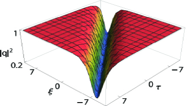
Figure 1: (Color online) The dark one-soliton propagation through homogenous fiber for parameters $k_{1}=1.5$, $k=a_{0}=D(\xi)=1$, $p=0$, $\delta=2$ and $\gamma=1$

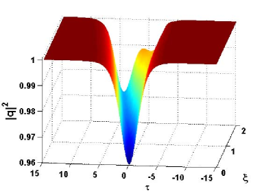
(a)

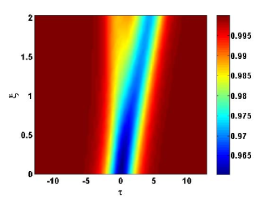
(b)

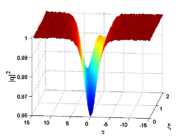
(c)

(d)

Figure 2: (Color online) Figs (a) and (b) show the dark soliton evolution and the formation of shcok wave. Figs (c) and (d) shows the stable propagation of the soliton and the shock wave formation in the presence of strong photon noise. The parameters of relevant physical quantities are $k_{1}=k=a_{0}=1$ $\delta=2$, $\gamma=1$and $p(\xi)=0$.

III.1 Direct numerical simulation

One of the essential aspect of a solitary wave is its stability on propagation. Unlike the conventional pulses of different form, the solitons are relatively stable, even in an environment subjected to external perturbations. Hence, in order to validate the signature of soliton, such as stable propagation over appreciable distance, and the stability against perturbation, we perform numerical simulation using split-step Fourier method. In order to check the solution stability of our dark soliton solutions, as a representative case, we consider the one soliton solution given by Eq. (7), and perform the stability analysis in two parts, (i) direct numerical simulation of propagation of soliton using Vc-MNLSE, and (ii) the propagation of soliton subject to perturbation such as the photon noise. Fig. 2 shows the numerical simulation of stable propagation of the dark soliton in the continuous back ground. Fig. 2a shows the stable propagation of soliton pulse, and followed the shock wave formation as a consequence of SS due to the intensity dependent group velocity ref:sschina . As of now, the propagation of soliton pulses have been considered in an ideal environment. However, there are numerous effects can contribute to instability in the soliton propagation. Therefore, it is very informative to study the stability of the soliton in an environment subject to external noise or perturbations. To this end, we generated a photon noise, which corresponds to $0.35\%$ of the continuous background. This is indeed an appreciable noise level, which can potentially perturb any propagation, as evident from the smooth pulse shown in Fig. 2a and the noisy pulse depicted in Fig. 2c. So, the initial condition for the simulation is the soliton profile with strong perturbation. Fig. 2c shows the simulation results for the same parameters as chosen earlier. It is very evident that the dark soliton show remarkable stability against strong perturbation. The formation of the shock wave can also be clearly observed in the simulation. Thus, one can draw out a conclusion that the dark soliton solution constructed through the Hirota method shows excellent stability, which has been confirmed through direct numerical simulations.

IV Two-soliton solutions

To get the dark two-soliton solution, the power series expansions for $G$ and $F$ are truncated as follows, $G=G_{0}(1+g_{1}+g_{2})$ and $F=1+f_{1}+f_{2}$. Then, back to bilinear Eqs. (3)-(4), we obtain

$$g_{0} =a_{0}e^{ik\tau-i\omega\int D(\xi)d\xi}, g(\xi) =e^{-\int p(\xi)d\xi}, \lambda =\frac{a_{0}^{2}}{2}[\delta-\gamma k]D(\xi), \omega =-\frac{\lambda}{D(\xi)}-\frac{k^{2}}{2}$$

$$g_{1} =\alpha_{1}\,e^{\theta_{1}}+\alpha_{2}e^{\theta_{2}}, f_{1} =e^{\theta_{1}}+e^{\theta_{2}}, g_{2} =A_{12}\alpha_{1}\alpha_{2}\,e^{\theta_{1}+\theta_{2}}, f_{2} =A_{12}e^{\theta_{1}+\theta_{2}}$$

$$\theta_{1} =k_{1}\tau-\omega_{1}\int D(\xi)d\xi, \theta_{2} =k_{2}\tau-\omega_{2}\int D(\xi)d\xi, \alpha_{1} =\frac{2\omega_{1}+2kk_{1}+ik_{1}^{2}}{2\omega_{1}+2kk_{1}-ik_{1}^{2}}, \alpha_{2} =\frac{2\omega_{2}+2kk_{2}+ik_{2}^{2}}{2\omega_{2}+2kk_{2}-ik_{2}^{2}}$$

$$\omega_{1}=\frac{1}{12k\gamma a_{0}^{2}-4k_{1}^{2}}(4kk_{1}^{3}+\gamma a_{0}^{2}k_{1}(-12k^{2}-3ikk_{1}+k_{1}^{2})\\ -\sqrt{(-k_{1}^{2}(4k_{1}^{4}+4a_{0}^{2}k_{1}^{2}(k\gamma-2\delta+3i\gamma k_{1})-\gamma a_{0}^{2}(39k^{2}\gamma-24k\delta+30ik\gamma k_{1}+\gamma k_{1}^{2})))})$$

$$\omega_{2}=\frac{1}{12k\gamma a_{0}^{2}-4k_{1}^{2}}(4kk_{1}^{3}+\gamma a_{0}^{2}k_{1}(-12k^{2}-3ikk_{1}+k_{1}^{2})\\ -\sqrt{(-k_{1}^{2}(4k_{1}^{4}+4a_{0}^{2}k_{1}^{2}(k\gamma-2\delta+3i\gamma k_{1})-\gamma a_{0}^{2}(39k^{2}\gamma-24k\delta+30ik\gamma k_{1}+\gamma k_{1}^{2})))})$$

$$A_{12}=-\frac{2i(\alpha_{1}-\alpha_{2})(\omega_{2}-\omega_{1}-kk_{1}+kk_{2})-(\alpha_{1}+\alpha_{2})(k_{1}-k_{2})^{2}}{2i(1-\alpha_{1}\alpha_{2})(\omega_{1}+\omega_{2}+kk_{1}+kk_{2})-(\alpha_{1}\alpha_{2}+1)(k_{1}+k_{2})^{2}}$$

The two-soliton solution can be written as,

$$q(\xi,\tau)=e^{-\int p(\xi)d\xi}\frac{g_{0}(1+g_{1}+g_{2})}{(1+f_{1}+f_{2})}$$ (9)

Using Eq. (9), the propagation of dark two-soliton through homogenous fiber is depicted in the Fig. (3)

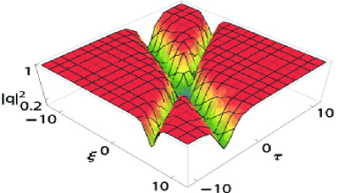
Figure 3: (Color online) The dark two-soliton propagation through homogenous fiber for parameters $k_{1}=-1.5$, $k_{2}=1.5$, $k=a_{0}=D(\xi)=1$, $p=0$, $\delta=1$ and $\gamma=0.2$.

IV.1 Two-soliton interactions

The interaction behaviors between two solitons in fibers can be revealed by the asymptotic states of soliton solution. Based on the two-soliton solution, we discuss the collision between dark solitons in inhomogeneous fibers. The asymptotic analysis of two soliton solutions are constructed as follows:

1) Before collision

(a)$S_{1}^{-}(\theta_{1}\sim 0,\theta_{2}\rightarrow-\infty)$

$$q(\xi,\tau)\rightarrow S_{1}^{-}=\frac{a_{0}e^{i\psi}}{2e^{\int p(\xi)d\xi}}[(1+\alpha_{1})+(\alpha_{1}-1)tanh(\frac{\theta_{1}}{2})]$$ (10)

(b)$S_{2}^{-}(\theta_{2}\sim 0,\theta_{1}\rightarrow\infty)$

$$q(\xi,\tau)\rightarrow S_{2}^{-}=\frac{a_{0}\alpha_{1}e^{i\psi}}{2e^{\int p(\xi)d\xi}}[(1+\alpha_{2})+(\alpha_{2}-1)tanh(\frac{\theta_{2}}{2}+\ln(\sqrt{A_{12}}))]$$ (11)

2)After collision

(a)$S_{1}^{+}(\theta_{1}\sim 0,\theta_{2}\rightarrow\infty)$

$$q(\xi,\tau)\rightarrow S_{1}^{+}=\frac{a_{0}\alpha_{2}e^{i\psi}}{2e^{\int p(\xi)d\xi}}[(1+\alpha_{1})+(\alpha_{1}-1)tanh(\frac{\theta_{1}}{2}+\ln(\sqrt{A_{12}}))]$$ (12)

(b)$S_{2}^{+}(\theta_{2}\sim 0,\theta_{1}\rightarrow-\infty)$

$$q(\xi,\tau)\rightarrow S_{2}^{+}=\frac{a_{0}e^{i\psi}}{2e^{\int p(\xi)d\xi}}[(1+\alpha_{2})+(\alpha_{2}-1)tanh(\frac{\theta_{2}}{2})]$$ (13)

From the asymptotic expressions before collision (10)- (11) and after collision (12)- (13), one can infer the elastic interaction and particle like behavior of solitons during the time of collisions between $S_{1}$ and $S_{2}$. The relevant physical quantities of solitons $S_{1}$ and $S_{2}$ before and after collisions are mentioned in Table 1.

Table 1: Physical quantities of solitons $S_{1}$ and $S_{2}$ before and after the collision.

Solitons	Velocities	Widths	Amplitudes	Energies
$s_{1}^{-}$	$\frac{\omega_{1}}{k_{1}}D(\xi)$	$\frac{1}{k_{1}}$	$|\frac{a_{0}(1+\alpha_{1})}{2e^{\int p(\xi)d\xi}}|$	$\frac{a_{0}^{2}(2-\alpha_{1}-\alpha_{1}^{*})}{k_{1}e^{2\int p(\xi)d\xi}}$
$s_{2}^{-}$	$\frac{\omega_{2}}{k_{2}}D(\xi)$	$\frac{1}{k_{2}}$	$|\frac{a_{0}\alpha_{1}(1+A_{12}\alpha_{2})}{e^{\int p(\xi)d\xi}(1+A_{12})}|$	$\frac{a_{0}^{2}(2-\alpha_{2}-\alpha_{2}^{*})}{k_{2}e^{2\int p(\xi)d\xi}}$
$s_{1}^{+}$	$\frac{\omega_{1}}{k_{1}}D(\xi)$	$\frac{1}{k_{1}}$	$|\frac{a_{0}\alpha_{2}(1+A_{12}\alpha_{1})}{e^{\int p(\xi)d\xi}(1+A_{12})}|$	$\frac{a_{0}^{2}(2-\alpha_{1}-\alpha_{1}^{*})}{k_{1}e^{2\int p(\xi)d\xi}}$
$s_{2}^{+}$	$\frac{\omega_{2}}{k_{2}}D(\xi)$	$\frac{1}{k_{2}}$	$|\frac{a_{0}(1+\alpha_{2})}{2e^{\int p(\xi)d\xi}}|$	$\frac{a_{0}^{2}(2-\alpha_{2}-\alpha_{2}^{*})}{k_{2}e^{2\int p(\xi)d\xi}}$

(a)

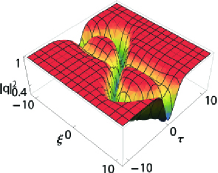
(b)

Figure 4: (Color online) The dispersion and nonlinearity managed dark solitons, (a) One-soliton (b) Two-soliton. Other physical quantities are $k=a_{0}=D(\xi)=Cos(0.3\xi)$, $p=0$, $\delta=2$ and $\gamma=1$.

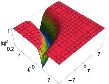
(a)

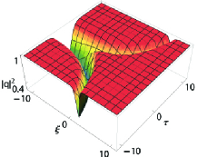
(b)

Figure 5: (Color online) The pulse compression of dark solitons, (a) One-soliton (b) Two-soliton. Other physical quantities are $k=a_{0}=D(\xi)=Exp(0.3\xi)$, $p=0$, $\delta=2$ and $\gamma=1$.

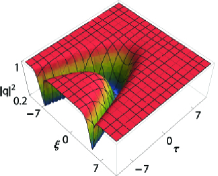
(a)

(b)

Figure 6: (Color online) The boomerang like dark solitons, (a) One-soliton, (b) Two-soliton. Other physical quantities are $k=a_{0}=D(\xi)=0.3+0.5\xi$, $p=0$, $\delta=2$ and $\gamma=1$.

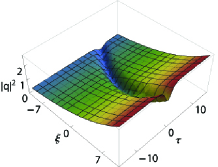
(a)

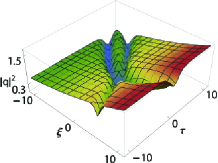
(b)

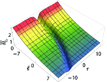
(c)

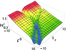
(d)

Figure 7: (Color online) The dark solitons propagation with gain, (a) One-soliton, (b) Two-soliton. The other parameters are $k=a_{0}=D(\xi)=1$, $p=-0.05$, $\delta=2$ and $\gamma=0.2$. The dark solitons propagation with loss, (c) One-soliton (d) Two-soliton with $p=+0.05$.

V Results and discussions

In the presented analytical work, we first investigated the constant propagation of dark soliton pulse in the homogeneous medium. In such system, the coefficient corresponding to dispersion and nonlinearity remains constant. Using Hirota Bilinear method, the analytical dark soliton solution corresponding to one and two are presented graphically in Figs. 1 and 3) via Eqs. (7)and (9) respectively. It is found that the dark soliton propagates without deformation in such homogeneous system, and its amplitude and velocity remains constant. In the following section, we examine the dynamical evolution of dark soliton for different physical effects in inhomogenous fibers with variable coefficients, dispersion and nonlinearity.

(a)

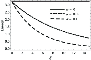
(b)

Figure 8: (Color online) Energy variation with gain/loss via the solution (8). (a) Gain with $p=-\sigma$, (b) Loss with $p=+\sigma$. The other relevant physical quantities are $k=a_{0}=\delta=D(\xi)=1$,$k_{1}=1.5$ and $\gamma=0.1$.

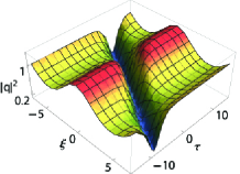
(a)

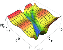
(b)

Figure 9: (Color online) The dark solitons propagation with periodic background, (a) One-soliton, (b) Two-soliton. The other physical quantities are $k=a_{0}=D(\xi)=1$, $p=0.1sin(0.7\xi)$, $R(\xi)=1$ and $S(\xi)=0.5$.

V.1 Periodic varying dispersion and nonlinearity

To study the dispersion-managed dark soliton by periodic perturbations, we consider a system with GVD parameter $D(\xi)$ and nonlinearity parameters $R(\xi)$ and $S(\xi)$ as a trigonometric periodic function. In this case, the solitons are oscillating without any compression or broadening and the pulse peak position and velocity vary periodically during the time of propagation. This kind of soliton is commonly called as a snaking soliton ref:61 ; ref:62 ; ref:63 ; ref:64 . Similar type of inhomogeneous behavior is observed in two-soliton solution as well. In all the cases, the dispersion and nonlinearity parameters are taken in the form of $a\cos(b\xi)$, where $a$ and $b$ are integers. Fig. 4) represents the one and two soliton pulse evolutions with periodically varying effects. It shows that the amplitude, energy and pulse width remains constants during the propagation of the pulse down the fiber.

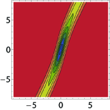
(a)

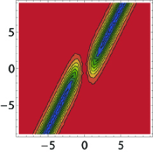
(b)

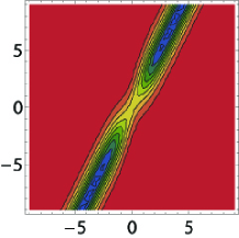
(c)

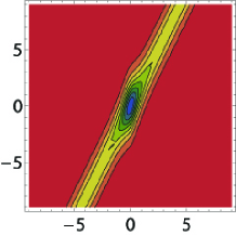
(d)

Figure 10: (Color online) Contour plot of nonlinear tunneling of dark one-soliton via solution (20). (a) Dispersion barrier with $D(\xi)=1+hsech[\xi-\xi_{0}]^{2}$, $R=1$, $S=0.2$ and $h=0.5$.(b) Dispersion well with $h=-0.9$.(c) Nonlinear barrier with $D(\xi)=1$,$R=1+hsech[\xi-\xi_{0}]^{2}$,$S=0.2(1+hsech[\xi-\xi_{0}]^{2})$ and $h=1$.(d) Nonlinear well with $h=-0.5$. Other physical quantities are $k_{1}=a_{0}=1$ and $\xi_{0}=0$.

V.2 Pulse Compression

Pulse compression (PC) is an important technique to produce ultrashort pulse in nonlinear fiber. It a mechanism of shortening the duration of the pulse. Techniques like soliton effect, adiabatic pulse compression, self-similar methods are few of the most popular pulse compression techniques. Generally, exponential dispersion and nonlinearity is preferred, as it found to compress soliton with a better a compression factor ref:65 ; ref:66 . In similar lines with the earlier report, we consider the dispersion and nonlinearity parameters of the form $c\exp(d\xi)$, where $c$ is the initial peak power and $d$ is an integer. The PC occurs, when the leading edge of the pulse is delayed by just the right amount to arrive nearly with the trailing edge ref:4 . The PC of one and two solitons are shown in the Fig. (5).

V.3 Boomerang Soliton

To study the parabolic profile of dark soliton, we choose the dispersion and nonlinearity parameters as $e+f\xi$, where $e$ and $f$ are integers. During the propagation, the soliton exhibits parabolic bending, and after the bending, the width of the soliton decreases gradually. Such type of soliton is commonly known as Boomerang soliton ref:62 ; ref:63 . For the above choices the one and two-soliton solutions are shown in the Fig. (6)

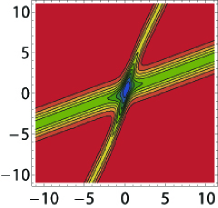
(a)

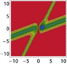
(b)

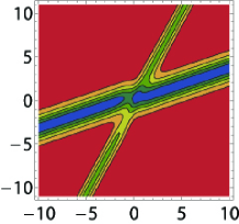
(c)

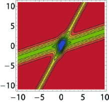
(d)

Figure 11: (Color online) Contour plot of nonlinear tunneling of dark two-soliton via solution (24). (a) Dispersion barrier with $D(\xi)=1+hsech[\xi-\xi_{0}]^{2}$, $R=1$,$S=0.2$ and $h=0.7$.(b) Dispersion well with $h=-0.9$.(c) Nonlinear barrier with $D(\xi)=1$,$R=1+hsech[\xi-\xi_{0}]^{2}$,$S=0.2(1+hsech[\xi-\xi_{0}]^{2})$ and $h=1$.(d) Nonlinear well with $h=-0.5$. Other physical quantities are $k_{1}=-0.8$, $k_{2}=0.8$, $a_{0}=1$ and $\xi_{0}=0$.

V.4 Gain/Loss

In the long distance optical fiber transmission system, the optical soliton will deform progressively as a result of fiber loss. In Eq. (1) coefficient $p(\xi)$ plays an important role in determining the amplification or absorption of the soliton pulse. The coefficient $p(\xi)=0$ corresponds to the case of fibers without any loss or gain. When $p(\xi)$ is a constant value, say $\sigma$, the solution represents the propagation of soliton pulse in a medium with constant gain or loss.

Figs. 7 illustrate the propagation of one and two solitons in a medium with gain/loss. When $\sigma<0(\sigma>0)$, the pulse undergoes the amplification (compression), and their amplitude of the pulse increases (decreases) as it propagates down the fiber. By varying the coefficient $p(\xi)$, the soliton amplification or absorption can be controlled. Fig. 8, represents the variation of dark soliton energy for some representative values of gain (Fig. 8a) and loss (Fig. 8b). It is quite evident that the energy monotonously increases (decreases) with gain (loss).

The gain/loss coefficient $p(\xi)$ can significantly influences the shape of the pulse background, in many recent works, different type of background profiles were considered ref:67 . Here, we demonstrated that the background undergoes a periodic oscillation. Fig. 9 shows the evolution of one- and two- solitons in a periodic background with $p(\xi)=g\sin(h\xi)$, where $g$ and $h$ are integers.

(a)

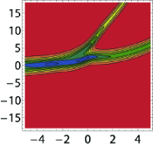
(b)

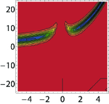
(c)

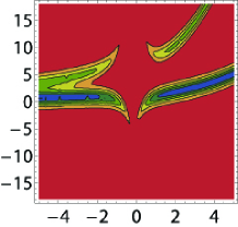
(d)

Figure 12: (Color online) Contour plot of nonlinear tunneling with exponential background. Dispersion barrier of (a) One soliton, (b) Two soliton, with $D(\xi)=d_{0}e^{-r\xi}+hsech[\xi-\xi_{0}]^{2}$,$R=R_{0}e^{-r\xi}$,$S=S_{0}e^{-r\xi}$ and $h=0.7$. Dispersion well of (c) One soliton, (d) Two soliton, with the same as for (a-b) except that $h=-0.9$. Other physical quantities are $d_{0}=R_{0}=1$ $S_{0}=0.2$,$r=-0.3$ $k_{1}=-0.8$, $k_{2}=0.8$, $k_{3}=-0.7$ and $\xi_{0}=0$.

VI Nonlinear tunneling effect

In the previous sections, we discussed about the impact of various physical effects and inhomogenous parameters in the one and two solitons. Now, we intent to investigate one of the dramatic nonlinear effects, known as the nonlinear tunneling (NL). Recently, many leading research works have been devoted to investigate the tunneling of solitons in different physical systems ref:48 ; ref:49 ; ref:50 ; ref:51 ; ref:52 ; ref:53 ; ref:54 ; ref:55 ; ref:56 ; ref:57 ; ref:58 ; ref:59 . All pioneering works have shown that the soliton can pass through the barrier without loss under a special conditions, which depends on the ratio between the height of the barrier and the amplitude of the soliton. The NL tunneling of soliton may create a new field of interest and feature wide applications in all-optical switches and logic circuits.

VI.0.1 Nonlinear tunneling without exponential background

To investigate the NL of Vc-MNLS dark soliton propagating through the dispersion barrier or well, we choose the dispersion and nonlinear parameter as follows:

$$D(\xi) =r_{0}\pm h\,sech^{2}(c(\xi-\xi_{0}))$$

$$R(\xi) =R_{0}$$

$$S(\xi) =S_{0}$$

In the above expressions, $h$ and $c$ represent the height and width of the barrier. $\xi_{0}$ represents the longitudinal co-ordinate indicating the location of the dispersion barrier/well. $D_{0}$, $R_{0}$ and $S_{0}$ are constant parameters. Here the positive or the negative sign of $\pm h$ denotes the barrier or the well. If $h=0$, the soliton is said to propagate through a homogenous fiber.

To investigate the soliton propagation through the nonlinear barrier or well, we consider the variable coefficients as follows:

$$D(\xi) =D_{0}$$

$$R(\xi) =R_{0}(r_{0}\pm h\,sech^{2}(c(\xi-\xi_{0}))$$

$$S(\xi) =S_{0}(r_{0}\pm h\,sech^{2}(c(\xi-\xi_{0}))$$

When the dark soliton is passing through the dispersion barrier, the intensity of the soliton grows and forms a peak at $\xi=\xi_{0}$. After passing through the barrier, the pulse retains its original shape as illustrated in Fig. 10a. For the case of dispersion well, the amplitude of the soliton vanishes and a valley is formed at $\xi=\xi_{0}$; after the tunneling, solitons are restored to their original shape as shown in Fig. 10b. On the other hand for nonlinear barrier/well, a valley is formed for nonlinear barrier and a peak is formed for well as evident from the Figs. 10c and 10d, respectively. In similar lines with one-soliton case, the NL tunneling of two solitons is demonstrated in the Figs. 11.

Due to the existing region of dark soliton ($0\leq A<a_{0}$), we can found that the height of the barrier (h) and amplitude of pulse (A) have a mutual relation in given soliton solutions. Thus we have studied the tunneling effect with suitable parametric choice of $h$. To investigate the dark soliton propagation through the dispersion barrier or well, we obtained a condition, where $h>0$ indicates the dispersion barrier, and $-1<h<0$ represents the dispersion well. Similarly, in the case of nonlinear barrier or well, we also obtained a condition, where $h>0$ indicates the nonlinear barrier, and $-1<h<0$ represents the nonlinear well.

VI.1 Nonlinear tunneling with exponential background

Now, we consider the tunneling effect with exponential background. This case is of particular importance, because, pulse tunneling through the exponential background generally results in the compression of the pulse. To investigate this special case, we consider the dispersion and nonlinear parameter as follows:

$$D(\xi) =D_{0}exp(-r\xi)\pm h\,sech^{2}(c(\xi-\xi_{0}))$$

$$R(\xi) =R_{0}exp(-r\xi)$$

$$S(\xi) =S_{0}exp(-r\xi)$$

Here, $r$ in the above expression represents the decaying parameter, which accounts for the exponential decay. Figs. (12a - 12b), represents the dark one and two solitons tunneling through dispersion barrier with exponential decay. It is observed that the amplitude of the soliton increases at $\xi=\xi_{0}$, and after tunneling through the barriers, the width of the soliton decreases gradually during propagation. Similarly, Figs. (12c - 12d) illustrates the dark soliton tunneling through dispersion well with exponential background for the case of one and two solitons. As it is evident that the amplitude of the soliton vanishes at $\xi=\xi_{0}$ and after emerging from the well, the soliton width compresses. From this result, one can infer that the input pulse can be compressed to a desired extent in a controllable manner by the proper choice of barrier or well parameters.

VII Summary and conclusion

In this paper, we have investigated a Vc-MNLS model with distributed dispersion, SPM, SS and linear gain/loss, which describes the dynamics of ultrashort pulse propagation in the inhomogeneous fiber systems. Using Hirota’s bilinear method, we analytically derived the exact one and two dark soliton solutions. We illustrated the effect of self-steepening such as shock wave formation during the propagation, which has been confirmed through direct numerical simulation. In order to validate the stability of the soliton solution, we numerically perform the stability analysis in the presence of photon noise, and our simulation illustrates the stable propagation of the dark soliton pulse. The collision behaviors of the dark soliton pulses in inhomogeneous fibers have also been discussed through asymptotic analysis.

For better insight about the effect of inhomogeneity, we exclusively studied the dynamical behavior of dark soliton with different physical effects up to the level of two-dark soliton interactions. In particular, we focused on the nonlinear tunneling of dark soliton through barrier/well. It has been found that the intensity of the tunneling soliton either forms a peak or valley and retains its shape after tunneling through barrier/well. We also identified the tunneling of dark soliton with exponential background tends to compress the pulse. Thus, in this paper, we attempt to give a complete study about the dark soliton dynamics in the Vc-MNLS model, by incorporating most of the physical effects. We believe the aforementioned results of the paper can serve as a reference for many future studies related to dark soliton.

VIII Acknowledgements

KP thanks DST, CSIR, NBHM, IFCPAR and DST-FCT Government of India, for the financial support through major projects. N. M. Musammil thanks UGC MANF, Government of India, for the financial support through Junior Research fellow. K.Nithyanandan thanks CNRS for post doctoral fellowship at Universite de Bourgogne, Dijon, France.

References

- (1) A. Hasegawa, F.D. Tappert, Appl. Phys. Lett. 23(1973)142
- (2) L.F. Mollenauer et al., Phys. Rev. Lett.45 (1980)1095
- (3) A. Hasegawa, Y. Kodama, Solitons in Optical Communications (Oxford University Press, Oxford, 1995)
- (4) G.P. Agrawal, Nonlinear Fiber Optics (Academic, New York, 2013)
- (5) F. Abdullaev, S. Darmanyan, P. Khabibullaev, Optical Solitons (Springer-Verlag, Berlin, 1991)
- (6) Yuri S. Kivshar, Barry Luther-Davies” Physics Reports. 298 (1998)81
- (7) P. Emplit, J. P. Hamaide, F. Reynaud, and A. Barthelemy, Opt. Commun. 62 (1987)374 .
- (8) A. M. Weiner, J. P. Heritage, R. J. Hawkins, R. N. Thurston, E. M. Kirschner, D. E. Leaird, and W. J. Tomlinson, Phys.Rev. Lett. 61 (1988)2445
- (9) Yuri S. Kivshar et al Chaos, Solitons and Fractals Vol. 4(1994) 1745
- (10) M. Mitchell, Z. Chen, M. Shih, and M. Segev, Phys. Rev. Lett. 77 490 (1996).
- (11) M.Mitchell and M. Segev, Nature (London) 387 (1997)880 .
- (12) Demetrios N. Christodoulides and Tamer H. Coskun. Phys. Rev. Lett.80 (1998)23
- (13) Xu T, Tian B, Li L L, L X and Zhang C Phys. Plasmas 15 (2008)102307
- (14) D. Mandelik, R. Morandotti, J. S. Aitchison, and Y. Silberberg, Phys. Rev. Lett. 92 (2004)093904
- (15) T. Tsurumi and M. Wadati, J.Phys. Soc. Jpn. 67 (1998)2294 .
- (16) M. Wadati and N. Tsuchida, J. Phys. Soc. Jpn. 75 (2006)014301.
- (17) A. Chabchoub, O. Kimmoun, H. Branger, N. Hoffmann, D. Proment, M. Onorato, and N. Akhmediev, Phys. Rev. Lett. 110 (2013)124101
- (18) F. De Martini, C. H. Townes, T. K. Gustafsson, and P. L. Kelley, Phys. Rev. 164(1967)312 .
- (19) D. Anderson and M. Lisak, Phys. Rev. A 27(1983)1393 .
- (20) J. R. de Oliveira and M. A. Moura,Phys. Rev. E 57(1998) 4751 .
- (21) Jeffrey Moses, Boris A. Malomed and Frank W. Wise1, Phys. Rev. A 76 (2007)021802(R) .
- (22) Seung-Ho Han and Q-Han Park, Phys. Rev. E 83(2011)066601 .
- (23) Yu Yu , Jia Wei-Guo, Yan Qing,Menke Neimule and Zhang Jun-Ping, Chin. Phys. 24(8) (2015) 084210
- (24) Min Li, Bo Tian, Wen-Jun Liu, Yan Jiang and Kun Sun, Eur. Phys. J. D 59 (2010)279
- (25) H.Q. Zhang, T. Xu, J. Li, B. Tian, Phys.Rev.E 77(2008)026605
- (26) M. Li, B. Tian, W.J. Liu, H.Q. Zhang, and P. Wang, Phys. Rev. E 81 (2010)046606.
- (27) V.N. Serkin, A. Hasegawa, Phys. Rev. Lett. 85, (2000)4502
- (28) I. Gabitov, E.G. Shapiro, S.K. Turitsyn, Phys. Rev. E 55(1997) 3624
- (29) Lakoba T I and Kaup D J, Phys. Rev. E 58 (1998)6728
- (30) Kruglov V I, Peacock A C and Harvey J D, Phys. Rev. Lett. 90(2003)113902
- (31) S.H. Chen, L. Yi, Phys. Rev. E 71 (2005)016606
- (32) Liu W J, B Tian and H Q Zhang, Phys. Rev. E 78(2008) 066613
- (33) Zhang H Q, Tian B, Liu W J and Xue Y S, Eur. Phys. J. D59 (2010)443
- (34) Hai-Qiang Zhang, Bao-Guo Zhai and Xiao-LiWang, Phys. Scr. 85(2012)015006.
- (35) Chao-Qing Dai, Zhen-Yun Qin and Chun-Long Zheng, Phys. Scr. 85 (2012)045007
- (36) Y. Kodama, M.J. Ablowitz, Stud. Appl. Math.64(1981) 225
- (37) K.J. Blow, N.J. Doran, Opt. Commun. 42 (1982)403 .
- (38) P. A. Subha et al., J. Modern Opt.54(2007)1827.
- (39) R. Hirota, The Direct Method in Soliton Theory (Cambridge University Press, Cambridge, 2004)
- (40) R. Radhakrishnan, M. Lakshmanan, J. Hietarinta, Phys. Rev. E 56 (1997)2213
- (41) T. Kanna, M. Lakshmanan, Phys. Rev. Lett. 86(2001)5043
- (42) W.J. Liu, B. Tian, H.Q. Zhang, L.L. Li, Y.S. Xue, Phys. Rev. E 77 (2008)066605
- (43) R.Radhakrishnan and M.Lakshmanan J.Phys.A:Math.Gen.28 (1995)2683.
- (44) K. Porsezian, K. Nakkeeran, Phys. Rev. Lett. 76 (1996)3955 .
- (45) A. Mahalingam and K. Porsezian Phys. Rev. E 64 (2001)046608.
- (46) S.G. Bindu, A. Mahalingam and K. Porsezian, Phys. Lett. A 286(2001)321.
- (47) Liu W J, B Tian, H Q Zhang, T Xu and H Li, Phys. Rev. A 79(2009) 063810
- (48) M. IdrishMiah, Optik 122(2011) 55.
- (49) A.C. Newell, J. Math. Phys. 19(1978) 1126
- (50) V.N. Serkin, T.L. Belyaeva, J. Exp. Theor. Phys. Lett. 74,(2001) 573
- (51) V.N. Serkin, V.M. Chapela, J. Percino, T.L. Belyaeva, Opt. Commun.192 (2001)237
- (52) Assaf Barak, Or Peleg, Chris Stucchio, Avy Soffer, and Mordechai Segev, Phys. Rev. Lett. 100(2008)153901
- (53) W.P. Zhong, M.R. Belic, Phys. Rev. E 81,(2010) 056604
- (54) C.Q. Dai, G.Q. Zhou, J.F. Zhang, Phys. Rev. E 85(2012) 016603
- (55) C.Q. Dai, Y.Y. Wang, Q. Tian, J.F. Zhang, Ann. Phys. 327 (2012)512
- (56) C.Q. Dai, Y.Y. Wang, J.F. Zhang, Opt. Express 18 (2010)17548
- (57) T.L. Belyaeva, V.N. Serkin, Eur. Phys. J. D 66(2012)153
- (58) V.N. Serkin, A. Hasegawa, T.L. Belyaeva, J. Mod. Opt. 60(2013) 116
- (59) . J.D. He, J.F. Zhang, J. Phys. A:Math. Theor 44 (2011)205203
- (60) M.S. Mani Rajan, J. Hakkim, A. Mahalingam and A. Uthayakumar, Eur. Phys. J. D 67 (2013)150.
- (61) Lei Wang, Min Li, Feng-Hua Qi and Chao Geng, Eur. Phys. J. D 69 (2015)108.
- (62) M J Ablowitz, S D Nixon, T P Horikis and D J Frantzeskakis. J. Phys. A: Math. Theor. 46(2013)095201
- (63) Malomed B A 2006 Soliton Management in Periodic Systems (Berlin: Springer)
- (64) A. Mahalingam, A. Uthayakumar and P. Anandhi, J Opt.42(3)(2013)182 .
- (65) . M.S. Mani Rajan, A. Mahalingam, A. Uthayakumar, J. Opt.14 (2012)105204
- (66) K.Porsezian, A.Hasegawa, V.N.Serkin, T.L. Belyaeva and R.Ganapathy, Phys. Lett. A 361(2007) 504
- (67) M N Vinoj and V C Kuriakose, J. Opt. A: Pure Appl. Opt. 6 (2004)63.
- (68) K. Nithyanandan, R. Vasantha Jayakantha Raja, and K. Porsezian, J. Opt. Soc. Am. B 30(2013) 178 .
- (69) Yu-Jie Feng et al., Phys. Scr. 90 (2015)045201