Thermal Pressure in Diffuse H₂ Gas Measured by
Herschel [C ii] Emission and FUSE UV H₂ Absorption

Abstract

UV absorption studies with the FUSE satellite have made important observations of H₂ molecular gas in Galactic interstellar translucent and diffuse clouds. Observations of the 158 $\mu$m [C ii] fine structure line with Herschel trace the same H₂ molecular gas in emission. We present [C ii] observations along 27 lines of sight (LOSs) towards target stars of which 25 have FUSE H₂ UV absorption. Two stars have only HST STIS C ii$\lambda$2325 absorption data. We detect [C ii] 158 $\mu$m emission features in all but one target LOS. For three target LOSs which are close to the Galactic plane, ${|\it b|}<$ 1^∘, we also present position-velocity maps of [C ii] emission observed by Herschel HIFI in on-the-fly spectral line mapping. We use the velocity resolved [C ii] spectra observed by the HIFI instrument towards the target LOSs observed by FUSE to identify [C ii] velocity components associated with the H₂ clouds. We analyze the observed velocity integrated [C ii] spectral line intensities in terms of the densities and thermal pressures in the H₂ gas using the H₂ column densities and temperatures measured by the UV absorption data. We present the H₂ gas densities and thermal pressures for 26 target LOSs and from the [C ii] intensities derive a mean thermal pressure in the range of $\sim$ 6100 to 7700 K cm^-3 in diffuse H₂ clouds. We discuss the thermal pressures and densities towards 14 targets, comparing them to results obtained using the UV absorption data for two other tracers C i and CO. Our results demonstrate the richness of the far-IR [C ii] spectral data which is a valuable complement to the UV H₂ absorption data for studying diffuse H₂ molecular clouds. While the UV absorption is restricted to the directions of the target star, far-IR [C ii] line emission offers an opportunity to employ velocity resolved spectral line mapping capability to study in detail the clouds’ spatial and velocity structures.

1. Introduction

The evolution of interstellar clouds can be broadly classified into four different evolutionary stages as diffuse atomic, diffuse molecular, translucent, and dense molecular clouds. The diffuse molecular and translucent clouds represent stages where the gas is primarily molecular hydrogen (Snow & McCall 2006) and UV radiation is present throughout the cloud. However, these diffuse and translucent H₂ clouds have been difficult to study throughout the Galaxy because H₂ does not emit under typical cloud temperatures, and CO, an important surrogate for H₂ in regions of higher extinction, is virtually absent due to UV photodissociation. Instead these clouds have primarily been studied locally (within $\sim$1 kpc) by visual and UV absorption lines against a bright background source. It has been proposed that Giant Molecular Cloud (GMC) formation, and thus the star formation rate in galaxies, is regulated by thermal pressure in the interstellar medium, or ISM (Cox 2005; Blitz & Rosolowsky 2006). Cloud formation over large scales depends on the thermal and dynamical state of the interstellar gas which in turn is modulated by heating and cooling rates, the gravitational potential, and turbulent and thermal pressures. Thus to more fully understand the thermodynamic state of the Galactic ISM and its relation to star formation, it is important to evaluate the pressure over the full extent of the disk. At present, the variation of thermal pressure throughout the Milky Way is observationally poorly defined. Gerin et al. (2015) have used the 158 $\mu$m [C ii] absorption spectra observed by HIFI towards a few selected Galactic objects to derive the thermal pressure in the diffuse ISM. In the solar neighborhood ($\sim$1 kpc) measurements of the thermal gas pressure have been made with C i UV absorption spectra towards a sample of about 89 selected target stars (Jenkins et al. 1983; Jenkins & Tripp 2001, 2011) and CO UV absorption towards 76 stars (Goldsmith 2013).

In this paper we develop a different approach to measuring the thermal pressure that relies on emission from [C ii], the fine structure emission line of ionized carbon at 158 $\mu$m (1.9 THz). To test this approach we observed spectrally resolved [C ii] with the Heterodyne Instrument in the Far Infrared (HIFI, de Graauw et al. (2010)) on the Herschel Space Observatory (Pilbratt et al. 2010) towards a sample of 25 lines of sight (LOS) with H₂ column densities previously derived from Far Ultraviolet Spectroscopic Explorer (FUSE) UV absorption observations (Rachford et al. 2002; Sheffer et al. 2008) and two from those observed in C ii$\lambda$2325 absorption by HST STIS (Sofia et al. 2004). The advantage of [C ii] is that it is observed in emission and so can probe the thermal pressure across the Milky Way. The large–scale Herschel [C ii] survey of the Milky Way (GOT C+; see Langer et al. (2010)) has shown that [C ii] emission can be apportioned among the different phases of the interstellar medium (Langer et al. 2010, 2014; Pineda et al. 2010, 2013; Velusamy et al. 2010; Velusamy & Langer 2014) and that a significant fraction is attributed to the emission from diffuse and translucent H₂ clouds.

Table 1Target lines of sight (LOS) observed by Herschel HIFI in [C ii] emission at 158 $\mu$$m$

Target Star		log $N$(H2)		log $N$(H i)		log $N$(C+)		T01(H2)	Distance
		cm-2	ref	1020 cm-2	ref	1017 cm-2	ref	(K)	(pc)
BD +31 643	G 160.491 -17.802	21.09 $\pm$ 0.19	1	21.38	1	–		73$\pm$48	150
HD 24534	G 163.081 -17.136	20.92 $\pm$ 0.04	1	20.73	1	17.49	7	57$\pm$4	2100
HD 34078	G 172.081 -02.259	20.88	2	21.19	5	—		75	450
HD 37021	G 209.006 -19.384	—		21.68	4	17.64	3,8	7011	560
HD 37061	G 208.925 -19.274	—		21.73	4	17.72	3,8	7011	640
HD 37903	G 206.851 -16.537	20.92 $\pm$ 0.06	2,10	21.16	4	18.02	3,8,9	68$\pm$7	830
HD 62542	G 255.915 -09.237	20.81 $\pm$ 0.21	1	20.93	1	—		43$\pm$11	310
HD 73882	G 260.182 +00.643	21.11 $\pm$ 0.08	1	21.11	1	—		51$\pm$6	450
HD 94454	G 295.692 -14.726	20.76	2	0.00	5	17.50	7	74	300
HD 96675	G 296.616 -14.569	20.82 $\pm$ 0.05	2	20.66	1	—		61$\pm$7	160
HD 115071	G 305.764 +00.152	20.69	2	20.91	6	17.87	7	71	2700
HD 144965	G 339.043 +08.417	20.79	2	20.52	5	17.52	7	70	510
HD 147683	G 344.857 +10.089	20.74	2	20.72	5	17.64	7	58	370
HD 147888	G 353.647 +17.709	20.47 $\pm$ 0.05	2,10	21.71	4	17.75	3,8,9	44$\pm$4	120
HD 152590	G 344.840 +01.830	20.51	2	21.37	4	17.80	3,8,9	64	3600
HD 154368	G 349.970 +03.215	21.46 $\pm$ 0.07	1	21.00	1	—		51$\pm$8	910
HD 167971	G 018.251 +01.684	20.85 $\pm$ 0.12	1	21.60	1	—		64$\pm$17	660
HD 168076	G 016.937 +00.838	20.68 $\pm$ 0.08	1	20.64	6	—		68$\pm$13	2000
HD 170740	G 021.057 -00.526	20.86 $\pm$ 0.08	1	20.96	6	—		70$\pm$13	330
HD 185418	G 053.602 -02.171	20.76 $\pm$ 0.05	1	21.19	4	17.64	9	105$\pm$6	1200
HD 192639	G 074.901 +01.480	20.75 $\pm$ 0.09	1,2	21.29	4	17.59	9	98$\pm$15	2100
HD 200775	G 104.062 +14.193	21.15	2	20.68	5	—		44	430
HD 203938	G 090.558 -02.234	21.00 $\pm$ 0.06	1	21.48	1	—		74$\pm$9	1040
HD 206267	G 099.290 +03.738	20.86 $\pm$ 0.04	1	21.30	1	17.85	7	65$\pm$5	860
HD 207198	G 103.136 +06.995	20.83 $\pm$ 0.04	1	21.14	1	17.51	3,8,9	66$\pm$5	1300
HD 207538	G 101.599 +04.673	20.91 $\pm$ 0.06	1	21.32	1	—		73$\pm$8	2000
HD 210839	G 103.828 +02.611	20.84 $\pm$ 0.04	1	21.15	1	17.79	7	72$\pm$6	1100

References: (1) Rachford et al. (2002, 2009)); (2) Sheffer et al. (2008); (3) Sofia et al. (2004); (4) Cartledge et al. (2004); (5) This paper: N(HI)= 5.8$\times$10²¹$E(B-V)$ -2N(H₂); (6) This paper: from the H i 21 cm $(l-V$) maps; (7) Jenkins & Tripp (2011); (8) Sofia et al. (2011); (9) Parvathi et al. (2012); (10) Rachford et al. (2009); (11) Assumed value.

By combining our HIFI [C ii] emission spectra with FUSE and STIS direct detections of H₂ or C⁺ in absorption we can better constrain many of the physical conditions in the clouds including the density and pressure of the H i and H₂ gas components. The availability of the thermal pressure and density in the literature from the C i and CO data on a subset of our [C ii] sample allows us to verify our approach. This validation is a step forward in the interpretation of [C ii] emission as a viable alternative to H₂ absorption studies of diffuse molecular clouds in the Galaxy.

An outline of our paper is as follows. In Section 2 we present the pointed observations towards the target selections and on-the-fly (OTF) spectral line mapping along three LOSs, and describe the data reduction. In Section 3 we present the [C ii] spectra for all 27 LOSs and spatial-velocity maps towards three targets. For the three mapped LOSs we compare the distributions of [C ii] with publicly available H i and ¹²CO or ¹³CO data. We analyze and interpret the [C ii] intensities to derive the thermal pressures and densities using H₂ column densities measured in the UV absorption. In Section 4 we present a comparison of the thermal pressures derived by [C ii] data with those available from the C i survey. We summarize our results in Section 5.

2. Observations

Our sample consists of the 25 FUSE targets with the highest H₂ column densities and two (HD 37021 & HD 37061) from the C ii$\lambda$2325 sample for which there are no FUSE H₂ absorption data. In Table 1 we list the target lines-of-sight (LOSs) selected from available FUSE and STIS UV absorption studies of H₂ (Rachford et al. 2002; Sheffer et al. 2008) and C ii$\lambda$2325 (Sofia et al. 2004) towards more heavily reddened diffuse clouds. The target distances in Table 1 are those available in Sheffer et al. (2008) or in more recent papers (e.g. Jenkins & Tripp 2011) and for a few are estimated from parallax given in the SIMBAD online data base. Though we do not use the distances in our analysis we include them here to give an overall view of the distribution of our target selection. The H i column densities and their reference sources are also given in Table 1. When available we use H i column densities derived from profile fitting of the naturally broadened wings of the Ly$\alpha$ absorption spectra (e.g. Diplas & Savage 1994; Cartledge et al. 2004). The H₂ rotational temperatures T₀₁(H₂) are from FUSE H₂ absorption data in Rachford et al. (2002, 2009) and Sheffer et al. (2008). For HD 37021 & HD 37061 we list the typical value $\sim$ 70 K. Although these two targets are severely confused by the overall emission from the Orion molecular cloud, we include them here as examples of PDR environments close to some of the FUSE target stars. We do not have the H₂ column density for these two target LOS but the C⁺ column density measurements are available from the STIS UV absorption Sofia et al. (2004, 2011); Parvathi et al. (2012). In Table 1 we list the C⁺ column densities for 15 targets, 8 estimated from UV C⁺ absorption spectra (Sofia et al. 2004 & 2011; Parvathi et al. 2012) and for 7 the C⁺ column densities are derived from scaling O i and/or S ii (Jenkins & Tripp 2011).

The observations of the fine-structure transition of C⁺ (²P_3/2 – ²P_1/2) at 1900.5369 GHz, reported here were made with the HIFI band 7b instrument (de Graauw et al. 2010) on Herschel (Pilbratt et al. 2010). The [C ii] spectra were obtained using the Wide Band Spectrometer with 0.22 km s^-1 velocity resolution over 350 km s^-1. For each target we used the Load CHOP (HPOINT) with a sky reference at $\sim$1$\fdg$4 to 2^∘ off from the target. To minimize the off source emission in the HPOINT spectra of 4 targets we used the OFF position from the GOT C+ survey (cf. Pineda et al. 2013). In the case of 8 targets which had a second target close to it within 2^∘ we used a common off position for each pair. This choice helped us to constrain any off source emission which, if present, would appear equally in both HPOINT spectra. For 12 targets we observed two HPOINT spectra using an off position at $\pm$1^∘ in right ascension and $\pm$1^∘ in declination.

HIFI Band 7 utilized Hot Electron Bolometer (HEB) mixers which produced strong electrical standing waves with characteristic periods of $\sim$320 MHz that depend on the signal power. Prior to the release of HIPE-13 the Level 2 [C ii] spectra provided by the Herschel Science Center show these residual waves. Our data were processed in HIPE-14 using the standard HIFI pipeline, which minimizes these residual waves. We used a new feature in HIPE-14 that mitigates the HEB electronic standing wave in band 7 (at the [C ii] frequency) as part of the standard pipe line. Any residual optical standing waves in the Level 2 spectra were removed by applying the fitHifiFringe task to the Level 2 data to produce satisfactory baselines. The H– and V–polarization data were processed separately and combined only after applying fitHifiFringe. We also extracted the OFF-source spectrum to examine and correct for any [C ii] spectral contamination due to the OFF–source subtraction.

For three targets (HD 115071, HD 168076 & HD 170740) which are close to the Galactic plane ($|b|$ $<$ 1$\fdg$0) we observed an OTF 6 arcmin longitudinal scan centered at the target star positions. All HIFI OTF scans were made in the LOAD-CHOP mode using a reference off–source position from the GOT C+ survey (cf. Langer et al. 2014) which were about 1 to 2 degrees away in latitude. The OTF 6 arcmin scans are sampled every 20 arcsec and the total duration of each OTF scan was typically $\sim$2000 sec.

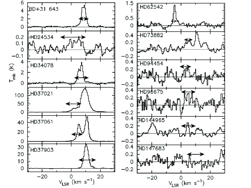
Figure 1.— HIFI pointed observation spectra of [C ii] 158 $\mu$m emission towards 12 FUSE target stars with names in the upper left corner of each spectrum. The horizontal double arrows mark the V_LSR range of CH, CH⁺ or atomic line absorption velocities available in an online catalog (Welty 2016) except for HD 73882 (Ritchey et al. 2011; Lacour et al. 2005).

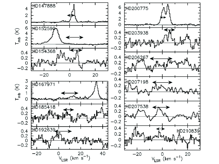
Figure 2.— HIFI pointed observation spectra of [C ii] 158 $\mu$m emission towards 12 FUSE target stars with names in the upper left corner of each spectrum. The horizontal double arrows mark the V_LSR range of CH, CH⁺ or atomic line absorption velocities available in an online catalog (Welty 2016) or in other resources, such as: Ritchey et al. (2011) for HD 154368; Lacour et al. (2005) for HD 185418, HD 192639, HD 206267 & HD 207538; Federman et al. (1997) for HD200775.

We processed the OTF scan map data following the procedure discussed in Velusamy & Langer (2014). Using the HIPE-14 Level 2 data (which are already corrected for the HEB standing waves) the [C ii] maps were made as “spectral line cubes” using the standard mapping scripts in HIPE. Any residual HEB and optical standing waves in the “gridded” map spectra were minimized further by applying fitHifiFringe to the individual spectra in the gridded scan map. The H– and V–polarization data were processed separately and were combined only after applying fitHifiFringe to the gridded data. This approach minimizes the standing wave residues in the scan maps by taking into account the standing wave differences between H– and V–polarization. We then used the processed spectral line data cubes to make longitude–velocity ($l$–$V$) maps of the [C ii] emission as a function of the longitude range in each of the 3 OTF scan observations. For HIFI observations we used the Wide Band Spectrometer (WBS) with a spectral resolution of 1.1 MHz for all the scan maps. The final $l$–$V$ maps presented here were restored with a velocity resolution of 1 km s^-1.

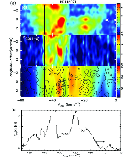
Figure 3.— HD 115071 (G305.764-0.152): (a) l–V maps of [C ii] 158 $\mu$m emission H i, and CO. The position offset zero corresponds to the target star. The H i 21 cm data are from the SGPS (McClure-Griffiths et al. 2005), ¹²CO (1-0) data are taken from the ThrUMMS survey (Barnes et al. 2011). Longitude-offset zero corresponds to $l$ = 305.7642^∘. The black vertical line represents the tangent velocity (see text). The brightness (T_mb K) scales for the images are indicated by the color bars. [C ii] emission contours are overlaid on the image of the H i 21 cm emission and the contour levels (T_mb) are 1, 2, 3, 4, 5, and 6 K. b: [C ii] spectrum towards the target star (at zero longitude-offset) observed by HIFI in the pointed observation. The horizontal double arrow marks the V_LSR range of CH absorption (from Andersson et al. 2002).

At 1.9 THz the angular resolution of the Herschel telescope is 12^′′, but the [C ii] OTF observations employed 20^′′ sampling. Such fast scanning results in an undersampled scan, and broadening of the effective beam size along the scan direction (Mangum et al. 2007). Therefore all [C ii] maps have been restored with an effective beam size corresponding to twice the 20^′′ sampling interval along the scan direction. Thus the shorter integration time per pixel in the final OTF maps restored with an 40^′′ beam and 1 km s^-1 wide channels yields an rms $\sim$0.22 K for T_mb which is slightly larger than in the HPOINT mode.

To compare the distribution of the C⁺ gas with the atomic and molecular gas we use the ¹²CO and H i 21 cm data in the southern Galactic plane surveys available in public archives. For HD 115071 the ¹²CO(1-0) data are taken from the Three-mm Ultimate Mopra Milky Way Survey (ThrUMMS) observed with the 22m Mopra telescope (Barnes et al. 2011) and the H i 21 cm data are taken from the Southern Galactic Plane Survey (SGPS) observed with the Australia Telescope Compact Array (McClure-Griffiths et al. 2005). For the other two targets we use H i 21 cm data from the VLA Galactic plane survey (VGPS) (Stil et al. 2006) and the ¹³CO(1-0) data from the Galactic Ring Survey (GRS) (Jackson et al. 2006).

3. Results

3.1. HIFI [C ii] emission spectra and (l–V) maps

The HIFI spectra of the velocity resolved [C ii] far-IR spectral line emission towards all targets in our sample are shown in Figures 1 to 5. The spectra are shown as main beam temperature, T_mb, plotted against the local standard of rest velocity, $V_{LSR}$, (we use a Band 7 main beam efficiency $\eta_{mb}$ = 0.585 and forward efficiency $\eta_{l}$ = 0.96). In these spectra, except for a few target LOSs, we detect weak to strong [C ii] emission features at multiple velocities. Unfortunately, the FUSE UV H₂ absorption data do not have velocity resolved spectral information to make direct comparison of the velocity features in the [C ii] emission spectra with the H₂ gas seen in UV absorption. However, to identify $V_{LSR}$ velocities of the [C ii] emission from the H₂ gas seen in absorption we can use available velocity resolved atomic and molecular UV absorption spectra towards our target stars, because these species are associated with diffuse gas. Here we primarily use CH or CH⁺, and if these are not available, atomic O i , Na i, or K i absorption spectra. We can then associate the $V_{LSR}$ velocity ranges over which absorption is detected in any of these spectra with the corresponding HIFI [C ii] emission spectral features. In the spectra in Figures 1 to 5 the UV absorption velocity range for each target derived from these tracers is marked by a horizontal double arrow. For most target stars we use the velocity resolved absorption data available in the online catalog of spectra compiled by Welty (2016) and the references therein. Whenever possible we use the high-resolution CH $\lambda$4300 line absorption spectra because, like most hydrides, it is present in diffuse molecular clouds (cf. Gerin et al. 2016) and shows a linear relationship between CH and H₂ column densities for A_V $<$ 4 mag. (e.g. Federman 1982; Rachford et al. 2002; Sheffer et al. 2008). Furthermore, for the [C ii] spectra in a few targets the identified V_LSR velocities near V_LSR=0 extend to positive and negative values which appear inconsistent with predicted velocity ranges for kinematic distances towards these target LOS if we assume circular Galactic orbits and a simple Galactic rotation curve. However, if we adopt the V_LSR velocities inferred from available directly observed UV absorption spectra it eliminates the need to model non-circular or peculiar velocities which will likely introduce more uncertainties.

By selecting only the absorption velocity range of the tracers of H₂ gas we can thus exclude any [C ii] emission features along the LOS that are not associated with the H₂ gas observed by FUSE. However, this exclusion is true only for LOS toward the outer Galaxy because we obtain a unique kinematic distance for any given V_LSR using the V_LSR–distance relationship derived by assuming circular Galactic orbits and using a simple Galactic rotation curve. For the LOS toward the inner Galaxy there is degeneracy in the V_LSR -distance relationship resulting in a near- and far-distance solution (e.g. Roman-Duval et al. 2009). In our FUSE–H₂ sample, of the 26 Galactic LOSs with [C ii] detections, 14 LOSs are toward the outer Galaxy with no distance ambiguity in associating [C ii] emission velocity with H₂ gas, while 12 are towards the inner Galaxy which are affected by the near- and far-distance ambiguity in the location of [C ii] emission whether it is between the target star and observer. Thus the V_LSR velocities, marked in Figs. 1 to 5, provide distances to two regions along each LOS, one at the far-distance (typically $>$ 10 kpc) beyond the target star and the second region at near-distance between the star and observer. In these target sights the [C ii] ] emission detected at a given $V_{LSR}$ can originate from the gas at the near-distance (between the target and observer) or at the far-distance beyond the target or may include emission from both near- and far-distance sources. We calculate the near- and far-distances for the $V_{LSR}$ velocities shown in the [C ii] spectra in Figs 1 to 5 and estimate their $z$-distance above or below the Galactic plane using their LOS Galactic latitude and far-distances which are typically $>$ 10 kpc. Except for HD 115071 and HD 192639, in all other target LOSs any gas at the far-distance would be located at $|z|$ $>$ 150 pc (up to a few kpc in many cases) where little diffuse H₂ gas is likely be present (Velusamy & Langer (2014) derived a scale height of 100 pc for diffuse H₂ using the GOT C+ [C ii] survey–see their Figure 15 and Table 3). Therefore, we conclude that for all but two LOS, the [C ii] emission identified by the $V_{LSR}$ velocities do not contain much, if any, contamination from any other sources beyond the target stars. In the case of HD 115071 and HD 192639 the far-distance gas if present would be at $z$ = 25 pc and 100 pc, respectively. If the emissions in the near- and far distances are roughly equal, the [C ii] intensities, which are assumed to be in the near-distance in our analysis, are overestimated by a factor of two. In this case the thermal pressures derived from [C ii] intensities for these two LOSs (Table 2) assuming all emission is in front of the target star are higher than the mean value for thermal pressure (see Section 4.1). On the other hand, if we have to correct their [C ii] intensities for contribution from far-distance gas their thermal pressures would be lower but still consistent with our results and conclusions.

In each spectrum in Figs. 1 to 5 the baseline used is marked by the horizontal line through zero intensity. These baselines were first fitted in the HIPE data processing using the full useable velocity range ($>$ 160 km s^-1) as part of the fitHifiFringe task which also removes the residual standing waves in the spectra. For a few LOSs the baselines were then improved by fitting over a narrower velocity range ($\sim$ 50 km s^-1) centered near the V_LSR of the H₂ gas. We caution that some of the low level velocity features (T_mb $<$ 0.2 K) in the spectra may be residual standing waves and may not be real. It may be noted that the rms noise estimates (in Table 2) exclude the low level standing waves.

For three FUSE targets: HD 115071 (G305.764+0.152), HD 168076 (G016.937+0.837) and HD 170740 (G021.057-0.526), for which we have [C ii] HIFI OTF scan maps, we show pointed spectra and (l–V) maps in Figures 3 to 5. These three targets have low Galactic latitudes (within 1^∘ of the plane) and therefore for these regions there exist high angular resolution ancillary H i 21 cm and some CO map data. The [C ii] maps allow us to resolve spatially the diffuse H₂ gas detected in the LOS UV absorption spectra. The availability of the H i 21 cm and CO maps allow us to further characterize the diffuse H₂ molecular cloud. The (l–V) maps of [C ii] intensity in T_mb and the corresponding H i 21 cm and CO maps (when available) are shown as color maps in $T_{mb}$. The spectra shown in Figures 3 to 5 have lower rms noise than those in the (l–V) maps because of the longer integration used for the pointed observations compared to the OTF scans. Furthermore, [C ii] emission in these pointed spectra correspond to a narrow beam (12^′′$\times$12^′′) while the (l–V) maps have a larger beam size of (40^′′$\times$12^′′ ) (see Section 2).

All three (l–V) maps show a clear detection of [C ii] at the velocities of the H₂ absorption. In addition, we detect [C ii] features at velocities corresponding to the inner Galaxy and many have associated CO counterparts. However, for both HD 115071 and HD 170740 there is no detectable CO matching the H₂ absorption clouds, confirming that these are diffuse clouds with very little or no CO in them. Here we discuss only the [C ii] features associated with the FUSE H₂ absorption.

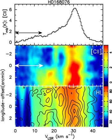
Figure 4.— HD 168076 (G016.937+0.837): Top panel: HIFI [C ii] velocity spectrum towards the target star (at zero longitude–offset) in a pointed observation. The double arrow marks the $V_{LSR}$ range of the K i absorption (Welty 2016 online catalog). Image panels: l–V maps of [C ii] 158 $\mu$m emission along with H i 21 cm. No CO map data are available for this target LOS. Longitude-offset zero corresponds to $l$ = 16.9373^∘. The H i 21 cm data are from the VGPS (Stil et al. 2006) observed with a beam of 1^′. The brightness (T_mb K) scales for the images are indicated by the color bars.

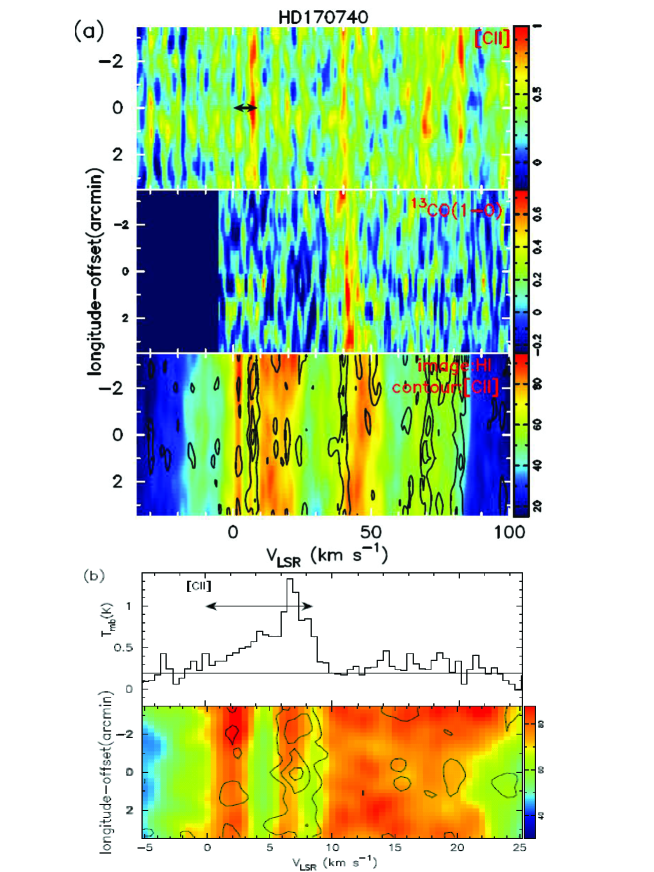
Figure 5.— HD 170740 (G021.057-0.526): (a) l–V maps of [C ii] 158 $\mu$m emission (top) along with ¹³CO (middle) and H i 21 cm (lower). The H i data are from the VGPS (Stil et al. 2006) and ¹³CO(1-0) from the GRS (Jackson et al. 2006). Longitude-offset zero corresponds to $l$ = 21.0574^∘. The brightness (T_mb K) scales for the images are indicated by the color bars. (b) Top panel: The HIFI [C ii] velocity spectrum towards the target star (at zero longitude-offset) observed in a pointed observation. The double arrow marks the $V_{LSR}$ range of the CH absorption (Ritchey et al. 2011). Image panel: Enlarged view of the l–V maps for the selected velocity range. The [C ii] intensity contours are overlaid on the H i 21 cm map.

3.2. [C ii] intensity analysis and H₂ cloud properties

A direct method to measure the density and temperature in H₂ clouds, and therefore their thermal pressure, is by observing several transitions of one or more gas probes that have the right energy spacing and collisional rate coefficients that probe the relevant parameter range. C⁺ has a fine-structure transition at 158 $\mu$m that arises from the ²P_3/2 level at an energy of 91.21 K, comparable to the kinetic temperatures in the diffuse and translucent clouds. It has been used to study the physical conditions in the ISM across the Galaxy (cf. Pineda et al. 2013; Langer et al. 2014) as well as in the Galactic Center (cf. García et al. 2016; Langer et al. 2017). Because C⁺ has only one fine-structure transition, [C ii] emission can only be used to derive one of three key physical parameters of the gas, either density, kinetic temperature, or column density as a function of the other two. For example, Gerin et al. (2015) derive the thermal pressures using C⁺ column densities measured from the [C ii] absorption data, with auxiliary assumptions about density, temperature, and the H i source. However, in the case of [C ii] observed in emission, as shown by Langer et al. (2014), there are regimes in density–temperature space where [C ii] can be used to estimate the product of density and temperature, or the thermal pressure, $P_{th}$ = $nT$, if one knows the C⁺ or H₂ column density. (We adopt the notation $P_{th}$ in units of K cm^-3 to express pressure divided by Boltzmann’s constant). In an Appendix we extend the treatment of Langer et al. (2014) and give a general solution applicable to a wider range of cloud conditions. Here we employ this approach as it applies to the lines of sight to the FUSE target stars and compare the pressures derived from [C ii] emission to those using UV absorption lines.

3.2.1 [C ii] intensities in the H i and H₂ gas components

To determine the [C ii] spectral line intensities it is critical to use a $V_{LSR}$ window that realistically represents the range of H₂ absorption within the [C ii] velocity profile. The ranges over which the velocity integrated [C ii] intensities were obtained are indicated in the spectral line velocity profiles in Figures 1 to 5. In cases where the [C ii] velocity feature is blended with adjacent emissions (e.g. HD37021, HD37061HD 152590, HD 200775) we use multi-Gaussian fits to compute the integrated intensities. The integrated [C ii] intensities, $I$([C ii]) in K km s^-1, are given in column 3 in Table 2. $I$([C ii]) is detected at the 5-$\sigma$ level or better for most targets, for three at the 3- to 4-$\sigma$ level, with one non-detection for HD 147683. In a few cases the [C ii] detections are marginal considering the presence of other comparable velocity features in the spectra. Nevertheless, they are statistically significant for studying the thermal pressures as the marginal detections can be used to determine upper limits to thermal pressure.

The [C ii] intensities integrated over the $V_{LSR}$ ranges of the H₂ UV absorption, in addition to the emission from the H₂ cloud (C⁺ excited by H₂ collisions), includes some emission from the H i gas along the line of sight (C⁺ excited by H collisions). We can thus write the observed [C ii] intensity as

$$I([CII])_{obs}=\int T_{mb}dV=I([CII])_{\rm HI}+I([CII])_{\rm H_{2}}$$ (1)

where $I$([C ii])_HI and $I$([C ii])${}_{H_{2}}$ are the emission in the H i and H₂ clouds respectively. To analyze the [C ii] emission from just the H₂ cloud we follow the steps below: (1) Determine $I$([C ii])_obs by integrating [C ii] emission over the $V_{LSR}$ window; (2) Calculate $I$([C ii])_HI from $N$(H i) with an assumed C⁺ fractional abundance and cloud pressure; (3) Calculate $I$([C ii])${}_{H_{2}}$ correcting the observed [C ii] intensities for any contribution from the H i gas; and finally, (4) Calculate the thermal pressure $P_{th}$ and density n(H₂) using the [C ii] intensity in the H₂ gas, the measured H₂ column density and temperature.

We use the observed H i column densities listed in Table 1 to determine the [C ii] contribution from the H i clouds. In Figure 6 we show a scatter plot of the total [C ii] intensity ($I$([C ii])_obs) against the H i column density $N$(H i). We do not see any strong correlation to suggest that there is any dominant contribution to $I({\rm CII})_{obs}$ from the H i column densities. However, the lower envelope of the scatter plot suggests there is a small contribution to $I({\rm CII})_{obs}$ that increases slowly with $N$(H i) as indicated by the solid line in Figure 6. We can therefore use Eq. A.9 to quantify the H i contribution in terms of H i gas pressure and $N$(H i) as a proxy for $N$(C⁺) in the H i clouds. Here we adopt a value for C⁺ fractional abundance $x$(C⁺/H i) = $x$(C/H) = 2.2 $\times$10^-4 (see section 4.2).

Figure 6.— Scatter plot of the observed HIFI [C ii] intensity against the H i column density. The solid line shows a lower boundary to the [C ii] intensity as a function $N$(H i). The solid line also represents [C ii] intensities for an assumed thermal pressure of the lower boundary $P_{th}$ = 2000 K cm^-3 (in Eq. A.9 assuming x(C⁺/H i) = 2.2$\times$10^-4 -see text).

Jenkins & Tripp (2001) derived the thermal pressure in diffuse atomic clouds from absorption line measurements of neutral carbon towards 26 stars and find an average pressure of 2240 K cm^-3. In a recent survey towards 89 stars Jenkins & Tripp (2011) (hereafter referred to as JT2011) derive their thermal pressure using the UV C i absorption. The number distribution of their pressure estimates have a mean value of $P_{th}$ = 3800 K cm^-3. Because C i is present in H₂ molecular gas rather than in the atomic H i gas this value is more representative of diffuse molecular clouds. However, 10% of their sample (about 9 target LOSs) have much lower values in the range of 900 to 2500 with a mean of value of 2000 K cm^-3. Since the pressure in the H i gas is likely to be lower we assume the lower values in the JT2011 pressure distribution and for our analysis of [C ii] in H i gas adopt $P_{th}$ $\sim$2000 K cm^-3. The $I({\rm CII})_{\rm HI}$ computed using this value for thermal pressure in H i as a function of $N$(H i) is shown in Figure 6 as the solid line which also fits well the lower envelope of the observed [C ii] intensity versus $N$(H i). To determine $I$([C ii])_HI we use the low density solution (Eq. A.9). Thus, using a gas pressure $P_{th}$ = 2000 K cm^-3 for atomic clouds and expressing H i column density in units of 10²⁰ cm^-2, we can reduce Eq. A.9 to,

$$I({\rm CII})_{\rm HI}=3.3\times 10^{-2}N_{20}({\rm HI})\qquad\qquad{\rm K\,km\,s^{-1}}.$$ (2)

For each target LOS we estimate the ${\rm I}({\rm CII})_{HI}$ in the H i gas component from Eq. 2 using the respective H i column densities in Table 1 column 4. In principle we can now compute the $I({\rm CII})_{\rm H_{2}}$ using these values for $I({\rm CII})_{HI}$. However, it should be noted that the H i column density used in Eq. 2 corresponds to the entire path length between observer and the target star while the observed velocity integrated [C ii] emission is over a smaller path length limited to the narrow V_LSR range of the UV absorption features. Ideally we should use the H i column density integrated over the same V_LSR range used to measure the [C ii] intensity. The H i column density derived from extinction or $L\alpha$ observations represents an integration over a much wider V_LSR range, corresponding to that between heliocentric zero to target radial velocity while the diffuse H₂ cloud is located over a narrower velocity range. Therefore the H i contribution within the V_LSR range of the [C ii] emission is overestimated. Indeed for the three LOS for which we have high angular resolution H i spectra (Figs. 3 to 5) the fraction of $N$(H i) seen in extinction within the [C ii] emission V_LSR range is 68% (HD 170740), 12% (HD168076), and 60% (HD115071) of the total velocity range to the target. The [C ii] intensity from the H i for all our LOSs varies between 0.1 K km s^-1 to 1.7 K km s^-1. However it is not likely that all of this H i contribution is overlapping the H₂ gas component seen in the [C ii] emission. We can then assume the true value of the [C ii] intensity in the H₂ gas is between the total observed and that corrected for H i contribution; here we use the average value:

$$I({\rm CII})_{H_{2}}=I({\rm CII})_{obs}-0.5\times I({\rm CII})_{HI}$$ (3)

For the three LOSs for which we have higher angular resolution H i spectra the full (100%) ${\rm I}({\rm CII})_{HI}$ is subtracted. In Table 2 we give the observed [C ii] intensities integrated over the V_LSR range as indicated in the spectra in Figs. 1 to 5, [C ii] intensity from the H i gas component and the H i corrected [C ii] intensities (Eq. 3) in the H₂ gas, ${\rm I}({\rm CII})_{H_{2}}$. Half of the contribution in the H i gas is added to the uncertainty in the estimate of I(CII)${}_{H_{2}}$. The 1-$\sigma$ uncertainty in [C ii] intensity from rms noise alone is in the range 0.2 to 0.5 K km s^-1. The 1-$\sigma$ error in Table 2 includes the uncertainties from the noise and the estimated H i contribution.

3.2.2 [C ii] cloud intensities and H₂ cloud pressure & density

In Figure 7 we show the measured $I$([C ii])${}_{H_{2}}$ for each target LOS plotted against the respective $N$(H₂). The data in Fig. 7 show some scatter in the observed [C ii] emission for any given H₂ column density in the diffuse cloud. The lack of a tight correlation between the [C ii] intensities and H₂ column densities may be the result of a wide range of pressures in the individual LOSs and at high [C ii] intensities due to the influence of the target star itself creating a high pressure PDR environment. To understand better the scatter in Fig. 7 we estimate the predicted $I$([C ii])${}_{H_{2}}$ as a function of $N$(H₂) using Eq. A.8 (for the low density solution in Appendix A and using $N$(H₂) as proxy for $N$(C⁺)) for several values of thermal pressure in H₂ gas. As discussed in Section 4.1 in our $I$([C ii])${}_{H_{2}}$ – $N$(H₂) analysis, we use a constant value of $x$(C/H₂)= $4.4\times 10^{-4}$ for all target LOS to estimate $N$(C⁺) from the measured $N$(H₂). The solid lines in Figure 7 delineate the lines of constant thermal pressure in $I$([C ii])${}_{H_{2}}$ – $N$(H₂) space. For a majority of the LOSs the [C ii] intensities are consistent with those expected for thermal pressures between 5000 and 20000 K cm^-3 with a few high pressure H₂ clouds possibly located in a PDR environment excited by the target stars.

To analyze the thermal pressures and their distribution in our FUSE H₂ sample we determine the values of $P_{th}$ in each LOS. Since we have estimates of the H₂ gas temperatures (T₀₁) from the excited levels of H₂, $T_{01}$(H₂) for this analysis we do not use the the low density solution in Appendix A. Instead we use the general solution Eq. B.2 (from Appendix B) for the thermal gas pressure and density, substituting $N$(C⁺) = $4.4\times 10^{-4}N$(H₂), temperature functions $f$(T), $b$(T) with corresponding values for T₀₁ and using n_cr(H₂)= 4500 cm^-3, and $a_{0}$ =3.28$\times$10^-16:

$$P_{th}=\frac{150\times{\rm I}({\rm CII})_{H_{2}}}{f(T)N_{20}(H_{2})}\frac{1}{1-0.07\times b(T)I([{\rm CII}])_{H_{2}}/N_{20}({\rm H_{2}})}$$ (4)

where $P_{th}$ is the cloud pressure expressed in K cm^-3 and the temperature functions are $f(T)={T_{01}}^{-1}e^{-91.21/T_{01}}$; and $b(T)=1+0.5e^{91.21/T_{01}}$. Finally, the volume density $n$(H₂) is derived from the $P_{th}$ obtained from the general solution as

$$n(H_{2})=P_{th}/T_{01}\qquad\quad{\rm cm^{-3}}.$$ (5)

The derived pressures and densities are summarized in Table 2. The uncertainty includes only that in the [C ii] intensity and does not include the uncertainty in the H₂ column density, kinetic temperature, or C⁺ fractional abundance. In most cases the overall uncertainty is $\sim$ 20%. Note that the first term in Eq 4 is the same as the solution for the low density approximation. For 3 out of the total 26 LOSs the [C ii] intensities are too high, $I$([C ii])${}_{H_{2}}$/$N_{20}$(H₂) is $>$ 7, and for values beyond 7 the general solution (Eq. 4) fails. Therefore, for these three target LOSs (HD 37021, HD 37061 & HD 37903) we show the values derived from the low density approximation which gives a lower bound. These and a few other high pressure LOSs are identified with the spectral type of target star which is also the exciting source of a PDR environment as discussed in Section 4.3. In general as shown in Appendix B, the thermal pressure derived from the [C ii] emission intensity analysis used in this paper is also consistent with radiative transfer analysis.

Figure 7.— 158 $\mu$m [C ii] intensity from the H₂ gas as a function of H₂ column density. The predicted [C ii] intensity for a given H₂ column density for a range of molecular gas pressure is also plotted. The error bars for the [C ii] intensities include the uncertainty in subtracting the H i contribution and the noise in the spectrum. The solid lines show the expected [C ii] intensity as a function of H₂ column density for assumed thermal pressures (K km s^-1; Eq. A.8 in Appendix A) adopting x(C⁺/H₂) = 4.4$\times$10^-4.

Figure 8.— $I$([C ii])${}_{H_{2}}$/$N$(C⁺)${}_{H_{2}}$ versus $I$([C ii])${}_{H_{2}}$ using the data in Tables 1 & 2 (see text). $I$([C ii])${}_{H_{2}}$/$N$(C⁺)${}_{H_{2}}$ is a direct measure of thermal pressure, $P_{th}$, and the corresponding values (see Eq. 8) are marked on the Y-axis to the right. The crosses represent data points (FUSE–H₂ sample) for which the $N$(C⁺)${}_{H_{2}}$ is computed from $N$(H₂) using x(C⁺/H₂)= 4.4$\times$10^-4. Note that for the crosses we use the H₂ column density and the corresponding [C ii] intensity in the H₂ gas component along the LOS. The filled triangles represent data points (UV–C⁺ sample) for which the $N$(C⁺)${}_{H_{2}}$ is obtained using $N$(C⁺) from direct UV absorption studies (references in Table 1) and H₂ fraction $f$(H₂) fraction (see text). The ellipses show the distribution of the H₂ clouds in the $I$([C ii]) versus $P_{th}$ space from the lower left to upper right suggesting a population of clouds in an evolutionary sequence– from low density, low pressure to a high pressure regime.

Table 2HIFI [C ii] intensities and derived thermal pressures and densities: Comparison with UV C i and CO results

Target	$I$([C ii])	$I$([C ii])	$I$([C ii])	$P_{th}$1	$P_{th}$2	n(H2)1	n(H2)3	Notes
Star	K km s-1	K km s-1	K km s-1	$\times$103 K cm-3	$\times$103 K cm-3	$\times$102 cm-3	$\times$102 cm-3
	observed	in H i gas	in H2 gas	[C ii]	C i	[C ii]	CO
BD +31 643	19.8 $\pm$ 0.18	0.79	19.40 $\pm$ 0.43	86 $\pm$ 1.4	—	12 $\pm$ 0.2	—	PDR (B5 V)
HD 24534	1.82 $\pm$ 0.26	0.18	1.73 $\pm$ 0.27	9.3 $\pm$ 1.4	14.8	1.6 $\pm$ 0.2	1.6
HD 34078	13.3 $\pm$ 0.25	0.51	13.04 $\pm$ 0.36	96 $\pm$ 1.8	—	13 $\pm$ 0.2	—	PDR (O9.5 Ve)
HD 37021	101.5 $\pm$ 0.22	1.58	100.71 $\pm$ 0.82	400 $\pm$ 3.2	6.8	56 $\pm$ 0.5	—	PDR $\theta^{1}$ Ori B (B3 V)
HD 37061	118 $\pm$ 0.33	1.77	117.11 $\pm$ 0.95	375 $\pm$ 3.0	19.1	54 $\pm$ 0.4	—	PDR $\nu$ Ori (B0.5 V)
HD 37903	133.43 $\pm$ 0.22	0.48	133.19 $\pm$ 0.32	580 $\pm$ 1.4	40.7	85 $\pm$ 0.2	$<$ 0.3	PDR (B1.5 V)
HD 62542	3.23 $\pm$ 0.21	0.28	3.09 $\pm$ 0.25	31.1 $\pm$ 2.1	—	7.2 $\pm$ 0.5	—	PDR (B3 V)?
HD 73882	2.44 $\pm$ 0.42	0.43	2.23 $\pm$ 0.47	8.3 $\pm$ 1.7	—	1.6 $\pm$ 0.3	—
HD 94454	1.06 $\pm$ 0.2	-0.02	1.07 $\pm$ 0.20	7.2 $\pm$ 1.3	4.0	1.0 $\pm$ 0.2	0.2 - 1.0
HD 96675	1.41 $\pm$ 0.27	0.15	1.33 $\pm$ 0.28	7.8 $\pm$ 1.6	—	1.3 $\pm$ 0.3	0.8 - 4.0
HD 115071	1.48 $\pm$ 0.21	0.27	1.35 $\pm$ 0.25	10.0 $\pm$ 2.0	4.4	1.4 $\pm$ 0.3	0.1 -0.8
HD 144965	0.51 $\pm$ 0.2	0.11	0.46 $\pm$ 0.21	2.9 $\pm$ 1.3	6.3	0.4 $\pm$ 0.2	1.3 - 1.6
HD 147683	0.13 $\pm$ 0.31	—	—	—	7.8	—	2.5
HD 147888	2.54 $\pm$ 0.21	1.69	1.69 $\pm$ 0.87	27.8 $\pm$ 12.0	9.6	6.3 $\pm$ 2.7	4.0 - 5.0
HD 152590	2.42 $\pm$ 0.38	0.77	2.03 $\pm$ 0.54	29.0 $\pm$ 6.7	5.1	4.5 $\pm$ 1.0	0.3 - 1.3	PDR (O7.5 V)
HD 154368	3.2 $\pm$ 0.48	0.33	3.04 $\pm$ 0.51	10.2 $\pm$ 1.6	—	2.0 $\pm$ 0.3	1.0 -4.0
HD 167971	4.63 $\pm$ 0.33	1.31	3.97 $\pm$ 0.74	25.5 $\pm$ 4.1	—	4.0 $\pm$ 0.6	—	PDR (O8 Ib)
HD 168076	3.44 $\pm$ 0.26	0.14	3.37 $\pm$ 0.27	31.2 $\pm$ 2.2	—	4.6 $\pm$ 0.3	—	PDR (O4 V)
HD 170740	3.24 $\pm$ 0.21	0.30	3.09 $\pm$ 0.26	17.0 $\pm$ 1.4	—	2.4 $\pm$ 0.2	—
HD 185418	1.06 $\pm$ 0.29	0.51	0.80 $\pm$ 0.39	5.4 $\pm$ 2.5	2.6	0.5 $\pm$ 0.2	0.1 - 0.4
HD 192639	2.16 $\pm$ 0.33	0.64	1.84 $\pm$ 0.46	12.9 $\pm$ 3.1	4.8	1.3 $\pm$ 0.3	$<$ 0.8
HD 200775	38.5 $\pm$ 0.2	0.16	38.42 $\pm$ 0.22	140 $\pm$ 0.8	—	32 $\pm$ 0.2	—	PDR (NGC2023)
HD 203938	2.73 $\pm$ 0.25	1.00	2.23 $\pm$ 0.56	8.9 $\pm$ 2.1	—	1.2 $\pm$ 0.3	—
HD 206267	3.17 $\pm$ 0.37	0.66	2.84 $\pm$ 0.50	17.0 $\pm$ 2.7	4.4	2.6 $\pm$ 0.4	2.0 - 2.5
HD 207198	1.62 $\pm$ 0.37	0.45	1.39 $\pm$ 0.43	8.5 $\pm$ 2.5	4.3	1.3 $\pm$ 0.4	0.3 -0.8
HD 207538	2.06 $\pm$ 0.29	0.69	1.72 $\pm$ 0.45	8.4 $\pm$ 2.1	—	1.2 $\pm$ 0.3	—
HD 210839	1.12 $\pm$ 0.27	0.47	0.89 $\pm$ 0.36	5.0 $\pm$ 2.0	4.6	0.7 $\pm$ 0.3	0.5

Note: (1) This paper; (2) Jenkins & Tripp (2011); (3) Goldsmith (2013).

4. Discussion

4.1. Molecular Gas Pressure

To understand better the scatter in the [C ii] intensity versus H₂ column density in Figure 7 and the effect of assuming a value for the fractional C⁺ abundance $x$(C/H₂), we consider a slightly different approach for displaying the data. We can rewrite Eq. A.8 as

$$\frac{{\rm I}({\rm CII})_{H_{2}}}{N_{17}(C^{+})_{H_{2}}}=0.51\times 10^{-4}P_{th},$$ (6)

where $N$(C⁺)${}_{H_{2}}$, expressed in units of 10¹⁷ cm^-2, is the C⁺ column density in the H₂ gas corresponding to the column density $N$(H₂). Thus the ratio of [C ii] intensity to C⁺ column density is a direct measure of the thermal pressure. For the FUSE targets with measured H₂ column densities we can use $N$(C⁺)${}_{H_{2}}$ = $N$(H₂)$x$(C/H₂). Therefore to interpret the [C ii] intensities in terms of the measured $N$(H₂), it is necessary to assume a value of $x$(C⁺/H₂) which introduces considerable ambiguity in the derived parameters such as pressure and volume density. There exist large variations in $x$(C/H) values in the literature. For example, Esteban et al. (2013) fit a value $\sim$ 3.2$\times$10^-4 for the solar neighborhood from deep echelle spectrophotometry of Galactic H ii regions (Esteban et al. 2013; García-Rojas & Esteban 2007). Using the solar abundance of $x$(C/H) $\sim$ 2.8$\times$10^-4 as a reference Jenkins (2009) derives depleted ISM gas phase carbon abundance $\sim$ 1.8 to 2.2$\times$10^-4. Parvathi et al. (2012) measure the ISM gas and dust-phase carbon abundance along 15 Galactic lines of sight and find values of gas phase $x$(C/H) between 0.7 and 4.6$\times$10^-4. As seen from Table 1 in our sample there are 13 targets that have column densities of H₂ from FUSE and $N$(C⁺) from UV absorption studies. (We refer to the targets which have $N$(C⁺) from UV absorption studies as UV–C⁺ sample and those with H₂ absorption as FUSE–H₂ sample.) We can then use these targets to calibrate our data and estimate a more realistic value for x(C⁺/H₂) applicable to all LOSs in our diffuse H₂ sample using the following approach.

(1) First, for the targets in the UV–C⁺ sample, we use the fraction of H₂ along the line of sight, $f$(H₂) = 2$N$(H₂)/(2$N$(H₂)+$N$(H i)), derived from the FUSE H₂ and H i column densities, to estimate the column density fraction of C⁺ in H₂, $N$(C⁺)${}_{H_{2}}$ = $N$(C⁺)$f$(H₂) where the total $N$(C⁺) is listed in Table 1.

(2) We then correlate $N$(C⁺)${}_{H_{2}}$ and $N$(H₂) for these 13 targets. The slope of a linear fit to these data corresponds to $x$(C⁺/H₂). We find, $x$(C⁺/H₂) = (4.4$\pm$0.5)$\times$10^-4 which is within the range of depletion with respect to H ($x$(C/H) $\sim$ 1.8 – 2.2$\times$10^-4) derived by (Jenkins 2009) (note $x$(C/H₂) = 2$x$(C/H)) and in our analysis it is obtained by using a sub-set of the FUSE targets themselves.

In Figure 8 we plot the ratio $I$([C ii])${}_{H_{2}}$/$N$(C⁺)${}_{H_{2}}$ for each target LOS against its [C ii] intensity $I$([C ii])${}_{H_{2}}$. The data points shown as crosses represent the targets in the FUSE–H₂ sample for which the $N$(C⁺)${}_{H_{2}}$ are calculated using the H₂ column density and x(C⁺/H₂)= 4.4$\times$10^-4. To further demonstrate the reliability of this value for $x$(C⁺/H₂) in Fig. 8 we plot $I$([C ii])${}_{H_{2}}$/$N$(C⁺)${}_{H_{2}}$ versus $I$([C ii])${}_{H_{2}}$ using a subset of 14 targets for which we have both $N$(C⁺) data determined by STIS UV absorption studies and have HIFI [C ii] detections. The data points are shown as filled triangles representing the UV–C⁺ sample for which the $N$(C⁺)${}_{H_{2}}$ is obtained using $N$(C⁺) and $f$(H₂) as discussed above. It may be noted that this data set is not dependent on the assumed values for $x$(C/H₂). Thus the distribution of these data points (filled triangles) in $I$([C ii])${}_{H_{2}}$/$N$(C⁺) – $I$([C ii])${}_{H_{2}}$ space provides a “bench mark” for the data plotted using the measured $N$(H₂) (crosses). The thermal pressure shown along the Y-axis on the right side corresponds to the value of the [C ii] intensity to C⁺ column density ratio, $I$([C ii])${}_{H_{2}}$/$N$(C⁺), shown along the Y-axis on the left (see Eq. 6). The degree of overlap between the two sets of data (the crosses and filled triangles) can be regarded as an independent validation of the assumed value for $x$(C⁺/H₂) and our overall approach for estimating thermal pressure using the [C ii] intensities.

In a $I$([C ii])–$P_{th}$ representation, as shown in Figure 8, our FUSE H₂ sample points (crosses) are distributed from the lower left (low pressure regime with low [C ii] intensity) to upper right (high pressure regime with high [C ii] intensity). This relationship seems to indicate that our H₂ cloud sample represents a population of clouds in an evolutionary sequence. Thus the [C ii] brightness of the cloud is a good indicator of the evolutionary status of the cloud: low brightness tracing formation stages while the high brightness ones the more evolved clouds in which increase in thermal pressure due to increase in density, UV field and gravity become more important. Alternatively, the H₂ clouds in our FUSE sample could represent different environments, from low to high pressure regions.

Observational data on the diffuse H₂ cloud properties such as mass, density, kinetic temperature, thermal and turbulent pressures, and their chemical make up are key to understanding the evolution of gas phases in the ISM. Jenkins & Tripp (2011) have reviewed the status of the thermal gas pressure in diffuse H₂ clouds in the solar neighborhood. Their measurements of thermal pressure towards 89 target stars using the HST STIS absorption studies in the C i fine structure lines provide a large enough sample for comparison to our derivation of thermal pressures using the HIFI [C ii] emission in concert with the H₂ UV absorption data. There are a total of 15 target stars common to our FUSE H₂ sample and the JT2011 C i sample, and we have [C ii] detections in 14 of them ([C ii] was not detected in HD 147683 above a 5-$\sigma$ noise). In Figure 9 we compare the thermal pressures derived by JT2011 with those from [C ii] emission.

As seen in Figure 9 the thermal pressures derived from $I$([C ii]) and $N$(H₂) are typically higher than the corresponding C i values in JT2011. Part of this difference may be due to the sensitivity of [C ii] emission to the PDR and FUV environments, as discussed further in Section 4.3. To bring out this difference more clearly we compare in Figure 10 histograms of the number distribution of $P_{th}$ measured with [C ii] and C i. The distribution maximum occurs for thermal pressures $\sim$4000 to 5000 K cm^-3 in the C i sample and $\sim$7500 to 9000 K cm^-3 in the [C ii] sample. The peaks are similar enough that we can regard these sources as corresponding to the ISM pressure in diffuse H₂ gas along the LOS, while those with much higher thermal pressure, $P_{th}\geq$10⁴ K cm^-3, as due to target-related PDR conditions. This bias is greatly enhanced by the likelihood for many of the target stars to occur in regions of high gas density especially, because they are generally of early spectral type as identified in Table 2. The 158 $\mu$m [C ii] absorption measurements provides a more robust estimate of $N$(C⁺) (Gerin et al. 2015). The thermal pressures derived from these absorption data are also in the range of 3800 to 22,000 K cm^-3 with a median value of 5900 K cm^-3. These values are broadly consistent with our results from [C ii] emission spectra. However, there are several sources of uncertainties in all these comparisons.

Figure 9.— Comparison of the molecular gas pressure derived using the observed [C ii] intensities and H₂ column density with those derived by JT2011. The solid line represents the two pressures being equal.

Figure 10.— Number distribution of the molecular gas pressure (a) derived using the observed [C ii] intensities and H₂ column density , and (b) C i from JT2011.

In the FUSE–H₂ sample among the total of 26 LOSs for which we measured the thermal pressure using the [C ii] emission, six have $P_{th}$ $>$ 50,000 K cm^-3 and eight have 12,000 $<$ $P_{th}$ $<$ 30,000 K cm^-3 while 12 out of 26, have $P_{th}$ $\leq$ 10000 K cm^-3. In a sub-set of 14 LOSs common to both our [C ii] and JT2011 C i targets, seven LOSs measured with [C ii] and eleven measured with C i are in the low pressure regime with $P_{th}$ $<$ 10,000 K cm^-3. When we exclude the high pressure PDR gas ($P_{th}$ $>$ 10,000 K cm^-3) the mean thermal pressure measured by [C ii] is 7700 K cm^-3, which is about 1.5 times higher than 5200 K cm^-3, measured by using C i. The differences in distribution of thermal pressures measured with [C ii] and C i, as seen in the histograms in Figure 10, indicates the differences in their intrinsic sensitivity to tracing H₂ gas in diffuse clouds. Systematic effects in the analysis of [C ii] emission and C i absorption can lead to over-/under- estimating thermal pressures. For example, if low values for $x$(C⁺/H) and $x$(C⁺/H₂) are used $P_{th}$ is overestimated or the contribution to observed [C ii] intensity from H i is underestimated. Furthermore, the uncertainties in $P_{th}$ listed in Table 2 are due to that in our estimate of the [C ii] intensity in the H₂ gas which in turn is mostly due to that in the contribution from H i (see Section 3.2.1 & Eq. 3). Thus $P_{th}$ is likely overestimated by underestimating the H i contribution. Indeed if we use the lower limit to $P_{th}$ as given by the uncertainties in Table 2 in the FUSE–H₂ sample, we find 13 LOS with $P_{th}$ $<$ 10,000 K cm^-3 with a mean pressure of 6100 K cm^-3 which is in better agreement with C i results. We conclude that mean thermal pressure measured by [C ii] in diffuse H₂ gas is in the range of 6100 to 7700 K cm^-3.

4.2. H₂ volume densities

Goldsmith (2013) constrained the H₂ densities in diffuse molecular clouds using an excitation analysis of the UV absorption measurements of CO low lying rotational levels up to J=3 towards many of the targets in our sample. His procedure also uses the FUSE H₂ column densities that we use in our [C ii] analysis. He derives the H₂ density from the excitation temperatures of the CO rotational levels seen in absorption, assuming a kinetic temperature typical of such clouds (the results are not overly sensitive to $T_{kin}$ because the highest level observed, J=3, has an excitation energy of 33.2 K, much less than the typical $T_{kin}$ $\sim$ 70 K in the gas). The CO excitation analysis uses the column densities of the J = 1–0, 2–1, and 3–2 transitions, where available, and the more levels detected the better the estimate of density. In about 40% of the sources excitation temperatures for two transitions are available, and in about 17% all three were determined. When only one transition is detected only lower and upper limits on the densities can be determined. In Table 2 we list the H₂ gas densities along the target LOSs derived using the [C ii] intensities and the respective H₂ column densities [Eq. 5]. For comparison with the [C ii] measurements, in Table 2 we show the densities for 14 target LOSs derived from CO absorption data (Goldsmith 2013). In Figure 11 we show a scatter plot of the densities derived independently using the far-IR [C ii] and UV CO data. The vertical bars for the densities measured with the CO data represents the range of densities constrained by the upper and lower limits given by Goldsmith (2013). The plot shows a reasonable agreement considering the different assumptions in the two approaches and that two outliers with high densities are in the high pressure PDR gas.

Figure 11.— Comparison of the molecular gas densities derived using the observed [C ii] intensities and H₂ column density with those derived by Goldsmith (2013) from CO excitation. The vertical error bars represent the upper and lower limits and the downward arrow the upper limit in Goldsmith’s data. The solid line is defined by the two densities being equal.

4.3. Excess far-IR [C ii] emission towards the target stars

In a few cases the proximity of the target star to the absorbing H₂ cloud becomes important as the target star plays the role of an exciting source creating a dense bright PDR environment resulting in larger [C ii] intensities. In such cases the density and temperature structure within the H₂ cloud can vary significantly between the near– and far–side to the observer. These sources are readily distinguishable in UV by a rich spectrum of vibrationally excited H₂ observed by the STIS on HST (e.g. Meyer et al. (2001)). In our sample, in addition to HD37021 & HD 37061, which lie in a strong UV and likely dense PDR environment in the Orion molecular cloud, there are several other target LOSs (BD +31 643, HD 34078HD 37903, HD 147888, HD152590 and HD 200775) that have [C ii] emission greatly enhanced by the presence of the PDRs. These are easily distinguished by their extremely high thermal pressure, $P_{th}>$ 15000 K cm^-3 (see Table 2). The models for the PDR environment in HD 37903 (Gnaciński 2011), in HD 147888 (Gnaciński 2013) show high densities and temperature structure as a function of target distance on the near side of the cloud. In the case of HD37903 the populations of the excited H₂ rovibrational states are consistent with the high density ($\sim$10⁴ cm^-3) molecular gas located about 0.5 pc from the B1.5 V star. BD +31 643 is a binary B5 V in IC 438, a young cluster (cf. Olofsson et al. (2012)). HD 200775 is the illuminating source of the reflection nebula NGC 7023 (Federman et al. 1997). HD 34078 is a runaway star with a dense shell at the stellar wind/molecular cloud interface that shows CH absorption and pronounced CO emission at the same V_LSR velocities as the [C ii] emission (Boissé et al. 2009). Thus the presence of an enhanced UV field and ionization front in these target environments also enhance the [C ii] emission, thus yielding the high pressures we derived from [C ii] for these LOSs. The thermal pressures estimated from [C ii] intensities are underestimated, and represent likely lower bound. However, these targets require a detailed PDR modeling analysis using the temperature and density structures (cf. Gnaciński 2011).

4.4. $(l-V)$ maps of [C ii] , H i and CO emissions

The target HD 115071 is located towards the Crux spiral arm tangency and the (l–V) maps (Fig. 3a) show a snapshot of the [C ii] and H i emissions, and the absence of CO at V_LSR$\sim$ -45 km s^-1 which bring out the differences among them in spiral arm tangencies. The angular resolution of the the H i 21 cm map (SGPS beam size $\sim$ 2.2^′) is much lower than that of the CO or [C ii] maps, but has comparable velocity resolutions. Therefore, we can compare the velocity structures. Beyond the tangent velocity the [C ii] shows a relatively strong emission in contrast to that of H i (with no CO) consistent with the results reported by Velusamy et al. (2012, 2015) that the [C ii] emission at this velocity is tracing the compressed warm ionized medium (WIM) along this spiral arm tangency. The [C ii] emission in this feature delineating the compressed WIM is due to excitation by the electrons in contrast to the excitation by H₂ molecules in the features at V_LSR $>$ -45 km s^-1 seen association with CO. Similarly, in the (l–V) maps of HD 170740 we identify the enhanced [C ii] emission with no CO, seen at the highest velocities near the tangent velocity at V_LSR $\sim$ 80 km s^-1 as a likely WIM component. In all three (l-V) maps the relatively strong [C ii] emission features, which have associated CO, trace the spiral arms along the LOSs: the Scutum-Crux arm at V_LSR$\sim$ -45 to -30 km s^-1 (HD 115071), the Scutum arm at V_LSR velocities near $\sim$ 40 km s^-1 (HD 170740), the Perseus spiral arm at V_LSR near $\sim$ 20 km s^-1, and the Scutum and some of the Sagittarius-Carina arms at V_LSR $\sim$ 30 km s^-1 (HD 168076).

5. Summary

The pressure in diffuse clouds is an important parameter in understanding the processes that affect their origin and determine their evolution. In this paper we have shown how [C ii] emission can be used to determine the thermal pressure and density in diffuse H₂ gas that is not readily traced in CO or other species. The diffuse H₂ clouds can be identified by the presence of ionized carbon (C⁺) emission ([C ii]) without any CO emission. Thus [C ii] provides an additional tool to complement H₂ and C i studied by UV absorption towards bright stars.

In this paper, we present [C ii] observations along 27 LOSs towards target stars of which 25 have FUSE H₂ UV absorption data and demonstrate how it could be used to estimate the thermal pressure in diffuse H₂ clouds. We detect [C ii] 158 $\mu$m emission features in 26 of these LOSs. For three LOSs which are close to the Galactic plane ${|\it b|}<$1^∘ we also present longitude–velocity maps of [C ii] emission observed by HIFI in on-the-fly (OTF) spectral line mapping. We analyzed and correlated the [C ii] velocity components detected along these LOSs in terms of the diffuse H₂ gas seen in the UV absorption data. We use the intensities of the [C ii] velocity components along with the column density of the diffuse H₂ gas as seen in the UV to derive the thermal pressure and H₂ densities in the diffuse molecular clouds. The distribution of thermal pressure in diffuse H₂ clouds shows a peak at $\sim$ 7500 – 9000 K cm^-3. Our results provide a validation of the use of [C ii] line intensity as a measure of the H₂ gas in the diffuse H₂ molecular clouds. We illustrate that the [C ii] intensity in H₂ clouds is a direct measure of the thermal pressure and that it traces the low– and high–pressure regimes in molecular cloud evolution.

Unlike the UV absorption studies which are limited to a pencil-like beam towards the direction of the target star, far-IR [C ii] line emission offers a much broader opportunity to study the diffuse H₂ gas over a cloud and throughout the Galaxy. Spectral line mapping has the further advantage allowing us to study in detail their spatial and velocity structures. We present examples of such spectral line map data towards three target LOSs. This use of [C ii] is particularly important in view of the new and enhanced opportunities from sub-orbital observations including SOFIA.

Appendix A A. Low density solution

Here we derive an equation to relate $I$([C ii]) to the thermal pressure under some realistic restrictions on the gas kinetic temperature. In the optically thin limit (see Equation 25 in Goldsmith et al. 2012), the [C ii] intensity, $I$([C ii]) is given by

$$I({\rm[CII]})=\int T_{A}dv=a_{0}N_{3/2}({\rm C^{+}})\,\,{\rm(K\,km\,s^{-1})},$$ (A1)

where

$$a_{0}=\frac{hc^{3}A_{3/2,1/2}}{8\pi k\nu_{3/2,1/2}^{2}}=3.28\times 10^{-16}\,\,{\rm(K\,km\,s^{-1}\,cm^{-2})},$$ (A2)

$A$= 2.3$\times$10^-6 s^-1, is the Einstein A-coefficient, the frequency $\nu_{3/2,1/2}$=1.9005 THz, and $N_{3/2}$ is the column density of the upper state in cm^-2. The units for $I$([C ii]) are K km s^-1. For a uniform medium we can write $N_{3/2}$(C⁺)=$n_{3/2}$(C⁺)$L$, where $L$ is the path length in cm, and $n_{3/2}$(C⁺) is the number density of ionized carbon in the upper ²P_3/2 state. For a two level system, in the optically thin regime, $n_{3/2}$(C⁺) can be solved exactly, yielding

$$n_{3/2}({\rm C^{+}})=\frac{n_{tot}({\rm C^{+}})}{1+0.5[1+n_{cr}(X)/n(X)]e^{\Delta E/T_{k}}},$$ (A3)

where $n_{tot}$(C⁺) is the total carbon ion density, $n$(X) is the density for X, the dominant collision partner (H, H₂, or e), $n_{cr}$(X) is the critical density of X, $T_{k}$ is the kinetic temperature, and $\Delta E$ =91.21 K, is the excitation energy of the ²P_3/2 state in Kelvins. Combining these terms yields

$$I({\rm[CII]})=\frac{a_{0}N({\rm C^{+}})}{1+0.5[1+n_{cr}(X)/n(X)]e^{\Delta E/T_{k}}}\,\,{\rm(K\,km\,s^{-1})}.$$ (A4)

In the low density limit where $n/n_{cr}<<$1, Equation A4 simplifies to,

$$I({\rm[CII]})=2a_{0}N({\rm C^{+}})\frac{n(X)e^{-\Delta E/T_{k}}}{n_{cr}(X)}\,\,{\rm(K\,km\,s^{-1})},$$ (A5)

which can be rewritten in terms of the thermal pressure $P_{th}^{0}$(X) =$n$(X)$T_{k}$, where X designates H or H₂, and the pressure is in units of K cm^-3.

$$I({\rm[CII]})=2a_{0}N({\rm C^{+}})\frac{P_{th}^{0}(X)}{n_{cr}({\rm X})}f(T_{k})\,\,{\rm(K\,km\,s^{-1})},$$ (A6)

where we use $P^{0}$ to denote the thermal pressure in the low density limit. The term $f$($T_{k}$)=$T^{-1}_{k}e^{-\Delta E/T_{k}}$ is plotted in Figure A.1. As discussed in Langer et al. (2014) it can be set to a constant value of 3.52$\times$10^-3 to within $\pm$15% over the temperature range 45 to 200K, which is the typical temperature range for [C ii] emission. The resulting approximate solution for the pressure in the low density limit is

$$P_{th}^{0}({\rm X})=4.14\times 10^{17}\frac{I({\rm[CII]})n_{cr}(X)}{N({\rm C^{+}})}\,\,({\rm K\,cm^{-3}}).$$ (A7)

The critical density for H₂ with an ortho-to-para ratio of one is $\sim$4.5$\times$10³ cm^-3 at $T_{k}$= 100K (Wiesenfeld & Goldsmith 2014) and is relatively insensitive to temperature, resulting in

$$P_{th}^{0}({\rm H_{2}})=1.96\times 10^{4}\frac{I({\rm[CII]}}{N_{17}({\rm C^{+}})}\,\,({\rm K\,cm^{-3}}),$$ (A8)

where we have expressed the column density, $N$(C⁺), in natural units of 10¹⁷ cm^-2, $N_{17}$(C⁺). For atomic hydrogen regions $n_{cr}$(H) $\simeq$ 3.3$\times$10³ cm^-3 for typical cloud temperatures, $T_{k}\sim$100K (Goldsmith et al. 2012), and in H i clouds

$$P_{th}^{0}({\rm H})\simeq 1.32\times 10^{4}\frac{I({\rm[CII]}}{N_{17}({\rm C^{+}})}\,\,({\rm K\,cm^{-3}}).$$ (A9)

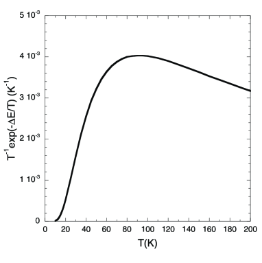
Figure A.1.— Dependence of $T^{-1}$exp(-91.21/T), which is proportional to the relative excitation rate to the ²P_3/2 level of C⁺, on the kinetic temperature. This term in the excitation rate varies by only 15% about its mean value of 3.52$\times$10^-3 over the range 45K $\leq T_{kin}\leq$ 200K, and by only 20% from 40K to 200K.

Appendix B B. General solution

It is possible to generalize the solution for the thermal pressure to all densities, i.e. arbitrary $n$(X)$/n_{cr}$(X), but under a slightly more restrictive temperature range. Fortunately this range, $T_{k}\sim$ 65 to 125 K, is appropriate for most [C ii] emission arising from atomic and molecular hydrogen regions. We start by rewriting Equation A4 in terms of the thermal pressure, $P_{th}$, for arbitrary $n$(X)/$n_{cr}$(X), which gives

$$I({\rm[CII]})=\frac{a_{0}N({\rm C^{+}})}{1+0.5e^{\Delta E/T_{k}}+[0.5n_{cr}(X)]/[P_{th}({\rm X})f(T)]}\,$$ (B1)

Solving for $P_{th}$ yields

$$P_{th}({\rm X})=\frac{0.5n_{cr}({\rm X})I([{\rm CII]})}{a_{0}f(T)N({\rm C^{+}})}\frac{1}{1-[b(T)I([{\rm CII}])]/[a_{0}N({\rm C^{+}})]},$$ (B2)

where $b(T)$=1+0.5e${}^{\Delta E/T_{k}}$. Note that the first term in Equation B2 is just the low density solution, $P_{th}^{0}$(X), given in Equation A7, so that

$$\frac{P_{th}}{P_{th}^{0}}=\Big{[}1-\frac{b(T)I([{\rm CII}])}{a_{0}N_{17}({\rm C^{+}})}\Big{]}^{-1}.$$ (B3)

We see from Equation B3 that $P_{th}^{0}$ underestimates the true thermal pressure for large values of $I$([C ii])/$N_{17}$(C⁺), which are characteristic of higher density regions. In Figure B.1 we plot $P_{th}/P^{0}_{th}$ in Equation B3 versus $I$([C ii])/$N_{17}$(C⁺) for a range of relevant kinetic temperatures. It is clear that the low density solution is excellent for $I$([C ii])/$N_{17}$(C⁺)$\leq$3, and reasonable up to a ratio of 5, but beyond that the solution to the pressure is sensitive to $T_{k}$.

If we do not know the kinetic temperature we see that from Figure B.1 over the important temperature range, 65 K to 125 K, we can set $b$(T) to a constant value and get a reasonable estimate of $P_{th}$. We find that fixing $b$(T) = 2.70 fits $P_{th}/P^{0}_{th}$ to within $\pm$25% over $T_{k}$ = 60 to 125 K, and to better than $\pm$20% over 65 to $\sim$110 K. This substitution, when used with a fixed value for $f(T_{k})$, yields an approximate expression for $P_{th}$(X) independent of density,

$$P_{th}=\Big{[}1-8.23\times 10^{-2}\frac{I([{\rm CII}])}{N_{17}({\rm C^{+}})}\Big{]}^{-1}{P_{th}^{0}},$$ (B4)

which has a solution for $I$([C ii])/$N_{17}$(C⁺)$\lesssim$12.1. We plot the ratio $P_{th}/P_{th}^{0}$ from Equation B.4 in Figure B.1 (dashed line) and it can be seen to provide a reasonable solution for the temperature range 65 to 125 K, when $T_{k}$ is not well known. We do not recommend estimating the true thermal pressure for very large values of the ratio $I$([C ii])$/N_{17}$(C⁺)$\geq$5, unless the kinetic temperature is reasonably well known.

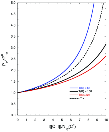
Figure B.1.— The ratio of the thermal pressure to the low density solution as a function of $I$([C ii])/$N_{17}$(C⁺) for a range of $T_{k}$ (solid lines). The approximate solution when the kinetic temperature is not known and a fixed value is adopted for $b(T_{k})$ is shown by the dashed line (Eq. B.4)

To test how well Equation B.4 reproduces the pressure given the ratio $I$([C ii])/$N$(C⁺) we compared the results to a radiative transfer model assuming a Large Velocity Gradient (LVG). We used the RADEX radiative transfer code (van der Tak et al. 2007) and the LAMDA data base (Schöier et al. 2005) to calculate $I$([C ii]) as a function of $P$ = $nT$ and column density, $N$(C⁺). In contrast to our optically thin solution, the RADEX code includes the effects of [C ii] opacity, $\tau$([C ii]). In the RADEX code we fixed $T_{k}$ = 100 K, the linewidth $\Delta V$ = 5 and 10 km s^-1, and the column density to $N$(C⁺) = 5$\times$10¹⁷ and 2$\times$10¹⁸ cm^-2 to represent a typical range in our data set. We then varied the density $n$(H₂) and calculate $P$=$nT$ and $I$([C ii]). We found good agreement within 15 – 20% between the approximate and RADEX solutions for $P_{th}$.

References

- Andersson et al. (2002) Andersson, B.-G., Wannier, P. G., & Crawford, I. A. 2002, MNRAS, 334, 327
- Barnes et al. (2011) Barnes, P. J., Yonekura, Y., Fukui, Y., et al. 2011, ApJS, 196, 12
- Blitz & Rosolowsky (2006) Blitz, L. & Rosolowsky, E. 2006, ApJ, 650, 933
- Boissé et al. (2009) Boissé, P., Rollinde, E., Hily-Blant, P., et al. 2009, A&A, 501, 221
- Cartledge et al. (2004) Cartledge, S. I. B., Lauroesch, J. T., Meyer, D. M., & Sofia, U. J. 2004, ApJ, 613, 1037
- Cox (2005) Cox, D. P. 2005, ARA&A, 43, 337
- de Graauw et al. (2010) de Graauw, T., Helmich, F. P., Phillips, T. G., et al. 2010, A&A, 518, L6
- Diplas & Savage (1994) Diplas, A. & Savage, B. D. 1994, ApJ, 427, 274
- Esteban et al. (2013) Esteban, C., Carigi, L., Copetti, M. V. F., et al. 2013, MNRAS, 433, 382
- Federman (1982) Federman, S. R. 1982, ApJ, 257, 125
- Federman et al. (1997) Federman, S. R., Knauth, D. C., & Lambert, D. L. 1997, ApJ, 489, 758
- García et al. (2016) García, P., Simon, R., Stutzki, J., et al. 2016, A&A, 588, A131
- García-Rojas & Esteban (2007) García-Rojas, J. & Esteban, C. 2007, ApJ, 670, 457
- Gerin et al. (2016) Gerin, M., Neufeld, D. A., & Goicoechea, J. R. 2016, ARA&A, 54, 181
- Gerin et al. (2015) Gerin, M., Ruaud, M., Goicoechea, J. R., et al. 2015, A&A, 573, A30
- Gnaciński (2011) Gnaciński, P. 2011, A&A, 532, A122
- Gnaciński (2013) Gnaciński, P. 2013, A&A, 549, A37
- Goldsmith (2013) Goldsmith, P. F. 2013, ApJ, 774, 134
- Goldsmith et al. (2012) Goldsmith, P. F., Langer, W. D., Pineda, J. L., & Velusamy, T. 2012, ApJS, 203, 13
- Jackson et al. (2006) Jackson, J. M., Rathborne, J. M., Shah, R. Y., et al. 2006, ApJS, 163, 145
- Jenkins (2009) Jenkins, E. B. 2009, ApJ, 700, 1299
- Jenkins et al. (1983) Jenkins, E. B., Jura, M., & Loewenstein, M. 1983, ApJ, 270, 88
- Jenkins & Tripp (2001) Jenkins, E. B. & Tripp, T. M. 2001, ApJS, 137, 297
- Jenkins & Tripp (2011) Jenkins, E. B. & Tripp, T. M. 2011, ApJ, 734, 65
- Lacour et al. (2005) Lacour, S., Ziskin, V., Hébrard, G., et al. 2005, ApJ, 627, 251
- Langer et al. (2017) Langer, W. D., Velusamy, T., Morris, M. R., Goldsmith, P. F., & Pineda, J. L. 2017, ArXiv e-prints
- Langer et al. (2010) Langer, W. D., Velusamy, T., Pineda, J. L., et al. 2010, A&A, 521, L17
- Langer et al. (2014) Langer, W. D., Velusamy, T., Pineda, J. L., Willacy, K., & Goldsmith, P. F. 2014, A&A, 561, A122
- Mangum et al. (2007) Mangum, J. G., Emerson, D. T., & Greisen, E. W. 2007, A&A, 474, 679
- McClure-Griffiths et al. (2005) McClure-Griffiths, N., Dickey, J., Gaensler, B., et al. 2005, ApJS, 158, 178
- Meyer et al. (2001) Meyer, D. M., Lauroesch, J. T., Sofia, U. J., Draine, B. T., & Bertoldi, F. 2001, ApJ, 553, L59
- Olofsson et al. (2012) Olofsson, G., Nilsson, R., Florén, H.-G., Djupvik, A., & Aberasturi, M. 2012, A&A, 544, A43
- Parvathi et al. (2012) Parvathi, V. S., Sofia, U. J., Murthy, J., & Babu, B. R. S. 2012, ApJ, 760, 36
- Pilbratt et al. (2010) Pilbratt, G. L., Riedinger, J. R., Passvogel, T., et al. 2010, A&A, 518, L1
- Pineda et al. (2013) Pineda, J. L., Langer, W. D., Velusamy, T., & Goldsmith, P. F. 2013, A&A, 554, A103
- Pineda et al. (2010) Pineda, J. L., Velusamy, T., Langer, W. D., et al. 2010, A&A, 521, L19
- Rachford et al. (2009) Rachford, B. L., Snow, T. P., Destree, J. D., et al. 2009, ApJS, 180, 125
- Rachford et al. (2002) Rachford, B. L., Snow, T. P., Tumlinson, J., et al. 2002, ApJ, 577, 221
- Ritchey et al. (2011) Ritchey, A. M., Federman, S. R., & Lambert, D. L. 2011, ApJ, 728, 36
- Roman-Duval et al. (2009) Roman-Duval, J., Jackson, J. M., Heyer, M., et al. 2009, ApJ, 699, 1153
- Schöier et al. (2005) Schöier, F. L., van der Tak, F. F. S., van Dishoeck, E. F., & Black, J. H. 2005, A&A, 432, 369
- Sheffer et al. (2008) Sheffer, Y., Rogers, M., Federman, S. R., et al. 2008, ApJ, 687, 1075
- Snow & McCall (2006) Snow, T. P. & McCall, B. J. 2006, ARA&A, 44, 367
- Sofia et al. (2004) Sofia, U. J., Lauroesch, J. T., Meyer, D. M., & Cartledge, S. I. B. 2004, ApJ, 605, 272
- Sofia et al. (2011) Sofia, U. J., Parvathi, V. S., Babu, B. R. S., & Murthy, J. 2011, AJ, 141, 22
- Stil et al. (2006) Stil, J. M., Taylor, A. R., Dickey, J. M., et al. 2006, AJ, 132, 1158
- van der Tak et al. (2007) van der Tak, F. F. S., Black, J. H., Schöier, F. L., Jansen, D. J., & van Dishoeck, E. F. 2007, A&A, 468, 627
- Velusamy & Langer (2014) Velusamy, T. & Langer, W. D. 2014, A&A, 572, A45
- Velusamy et al. (2015) Velusamy, T., Langer, W. D., Goldsmith, P. F., & Pineda, J. L. 2015, A&A, 578, A135
- Velusamy et al. (2012) Velusamy, T., Langer, W. D., Pineda, J. L., & Goldsmith, P. F. 2012, A&A, 541, L10
- Velusamy et al. (2010) Velusamy, T., Langer, W. D., Pineda, J. L., et al. 2010, A&A, 521, L18
- Welty (2016) Welty, D. E. 2016, in http://astro.uchicago.edu/dwelty/ew-atom.html
- Wiesenfeld & Goldsmith (2014) Wiesenfeld, L. & Goldsmith, P. F. 2014, ApJ, 780, 183