Variational discretization of the nonequilibrium thermodynamics of simple systems

Abstract

In this paper, we develop variational integrators for the nonequilibrium thermodynamics of simple closed systems. These integrators are obtained by a discretization of the Lagrangian variational formulation of nonequilibrium thermodynamics developed in Gay-Balmaz and Yoshimura [2017a], and thus extend the variational integrators of Lagrangian mechanics, to include irreversible processes. In the continuous setting, we derive the structure preserving property of the flow of such systems. This property is an extension of the symplectic property of the flow of the Euler-Lagrange equations. In the discrete setting, we show that the discrete flow solution of our numerical scheme verifies a discrete version of this property. We also present the regularity conditions which ensure the existence of the discrete flow. We finally illustrate our discrete variational schemes with the implementation of an example of a simple and closed system.

1 Introduction

Nonequilibrium thermodynamics is a phenomenological theory which aims to identify and describe the relations among the observed macroscopic properties of a physical system and to determine the macroscopic dynamics with the help of fundamental laws of thermodynamics (e.g. Stueckelberg and Scheurer [1974]). The field of nonequilibrium thermodynamics naturally includes macroscopic disciplines such as classical mechanics, fluid dynamics, elasticity, and electromagnetism.

It is well known that the equations of motion of classical mechanics, i.e., the Euler-Lagrange equations can be derived from Hamilton’s variational principle applied to the action functional associated to the Lagrangian of the mechanical system. One of the many features of the variational formulation is that it admits a discrete version which allows the derivation of structure preserving numerical schemes for the system. Such schemes, called variational integrators, (see, Wendlandt and Marsden [1997], Marsden and West [2001], Lew, Marsden, Ortiz and West [2004]) are obtained via a discrete version of Hamilton’s principle and are originally based on Moser-Veselov discretizations (see, Veselov [1988], Veselov [1991], Moser and Veselov [1991]). Several extensions of this method have been developed, for example to treat the case of forced mechanical systems (Kane, Marsden, Ortiz, and West [2000]) or nonholonomic mechanical systems (Cortés and Martínez [2001], McLachlan and Perlmutter [2006]).

In Gay-Balmaz and Yoshimura [2017a, b], we have developed a Lagrangian variational formulation for nonequilibrium thermodynamics which extends Hamilton’s principle of classical mechanics by allowing the inclusion of irreversible phenomena in both discrete and continuum systems, i.e., systems with finite and infinite degrees of freedom. The irreversibility is encoded into a nonlinear nonholonomic constraint given by the expression of the entropy production associated to all the irreversible processes involved. From a mathematical point of view, the variational formulation of Gay-Balmaz and Yoshimura [2017a, b] may be regarded as a nonlinear generalization of the Lagrange-d’Alembert principle used in nonholonomic mechanics, see e.g., Bloch [2003]. In order to formulate the nonholonomic constraint, to each irreversible process is associated a variable called the thermodynamic displacement that generalizes the thermal displacement introduced in Green and Naghdi [1991], following von Helmholtz [1884]. The introduction of such variables allows the definition of a corresponding variational constraint.

In the present paper, we develop variational integrators for nonequilibrium thermodynamics by discretizing the Lagrangian variational formulation developed in Gay-Balmaz and Yoshimura [2017a]. The resulting numerical schemes are thus extensions of the variational integrators of Lagrangian mechanics that enable to include irreversible phenomena. In the present paper, we restrict our discussions to the case of simple closed systems, i.e., closed systems in which one thermal scalar variable and a finite set of mechanical variables are sufficient to describe entirely the state of the system, though we will be able to develop our discrete theory to handle more general cases including the nonequilibrium thermodynamics of continuum systems.

A key property of variational integrators in Lagrangian mechanics is their symplecticity, meaning that the discrete flow, similarly to the flow of the continuous system, preserves a symplectic form. This ensures an excellent long-time energy behavior, see Hairer, Lubich, and Wanner [2006]. When irreversible effects are considered in the dynamics, the symplecticity of the flow may be lost at the continuous level, so there is no hope to discretize the system with a symplectic integrator, in general. In the paper, we shall present a property of the flow $F_{t}$ of simple closed systems in thermodynamics, which reduces to the symplecticity of the flow in absence of thermal effects. This property has the form

$$F_{t}^{\ast}\Omega-\Omega=-\mathbf{d}\int_{0}^{t}(F_{s}^{\ast}\omega)ds,\quad\text{for all $t$},$$

where $\Omega$ is an entropy-dependent symplectic form, $\omega$ is a one-form encoding the effects of friction and temperature, and $\mathbf{d}$ is the exterior derivative. We then show that our numerical scheme verifies a discrete version of this formula and therefore it reduces to a symplectic integrator in absence of thermal effects.

The paper is organized as follows. In Section 2 we review the fundamental laws governing the nonequilibrium thermodynamics of macroscopic systems by following the axiomatic formulation of Stueckelberg and Scheurer [1974]. Then, we also review the Lagrangian variational formulation of nonequilibrium thermodynamics developed in Gay-Balmaz and Yoshimura [2017a], which is an extension of Hamilton’s principle of classical mechanics that allows the inclusion of irreversible phenomena. In Section 3, after recalling some basic facts about variational integrators in Lagrangian mechanics, we propose a discrete version of the variational formulation for nonequilibrium thermodynamics of simple closed systems and deduce a variational integrator for these systems. In Section 4, we present a property of the flow $F_{t}$ of simple closed systems in thermodynamics, which reduces to the symplecticity of the flow in absence of thermal effects. Then we show that the discrete flow of our variational integrator verifies a discrete version of this property. We also study the regularity conditions which ensure the existence of the discrete flow. Finally, in Section 5, we illustrate the implementation of our integrator with an example of a simple system.

2 Nonequilibrium thermodynamics of simple systems

In this section we first review the fundamental laws governing the nonequilibrium thermodynamics of macroscopic systems. We follow the axiomatic formulation of thermodynamics developed by Stueckelberg around 1960 (see, for instance, Stueckelberg and Scheurer [1974]), which is well suited for the study of nonequilibrium thermodynamics as a general macroscopic dynamic theory that extends classical mechanics to account for irreversible processes. Needless to say, it is important to point out that this axiomatic formulation includes the description of systems out of equilibrium and is not restricted to the treatment of equilibrium states and transition from one equilibrium state to another. Then, we review the Lagrangian variational formulation of nonequilibrium thermodynamics from Gay-Balmaz and Yoshimura [2017a] which is an extension of Hamilton’s principle of classical mechanics to allow the inclusion of irreversible phenomena. For brevity, in this paper, we will restrict to the case of simple and closed systems.

2.1 Fundamental laws of nonequilibrium thermodynamics

For the macroscopic description of nonequilibrium thermodynamics, we have the following laws, see Stueckelberg and Scheurer [1974]:

• First law: For every system, there exists an extensive scalar state function $E$, called energy, which satisfies

  $$\frac{d}{dt}E(t)=P^{\rm ext}_{W}(t)+P^{\rm ext}_{H}(t)+P^{\rm ext}_{M}(t),$$

  where $t$ denotes time, $P^{\rm ext}_{W}(t)$ is the power due to external forces acting on the mechanical variables of the system, $P^{\rm ext}_{H}(t)$ is the power due to heat transfer, and $P^{\rm ext}_{M}(t)$ is the power due to matter transfer between the system and the exterior.

• Second law: For every system, there exists an extensive scalar state function $S$, called entropy, which obeys the following two conditions.

  • Evolution part:
    If the system is adiabatically closed, the entropy $S$ is a non-decreasing function with respect to time, i.e.,

    $$\frac{d}{dt}S(t)=I(t)\geq 0,$$

    where $I(t)$ is the entropy production rate of the system accounting for the irreversibility of internal processes.

  • Equilibrium part:
    If the system is isolated, as time tends to infinity the entropy tends towards a finite local maximum of the function $S$ over all the thermodynamic states $\rho$ compatible with the system, i.e.,

    $$\lim_{t\rightarrow+\infty}S(t)=\max_{\rho\;\text{compatible}}S[\rho].$$

In this context, a system is said to be closed if there is no exchange of matter between the system and the exterior, i.e., $P^{\rm ext}_{M}(t)=0$; a system is said to be adiabatically closed if it is closed and there is no heat exchanges between the system and the exterior, i.e., $P^{\rm ext}_{M}(t)=P^{\rm ext}_{H}(t)=0$; and a system is said to be isolated if it is adiabatically closed and there is no mechanical power exchange between the system and the exterior, i.e., $P^{\rm ext}_{M}(t)=P^{\rm ext}_{H}(t)=P^{\rm ext}_{W}(t)=0$.

By definition, the evolution of an isolated system is said to be reversible if $I(t)=0$, namely, the entropy is constant. In general, the evolution of a system is said to be reversible, if the evolution of the total isolated system with which it interacts is reversible.

In this paper, we only consider simple and closed systems. By definition, a simple system¹ is a system where one (scalar) thermal variable $S$ and a finite set $(q^{i},\dot{q}^{i})$ of mechanical variables are sufficient to describe entirely the state of the system, and we assume that there is no power due to matter transfer $P^{\rm ext}_{M}$ between the system and the exterior since the system is closed.

2.2 Variational formulation for nonequilibrium thermodynamics

Consider a simple closed system described by a mechanical variable $q\in Q$ and one entropy variable $S\in\mathbb{R}$. Let $L=L(q,\dot{q},S):TQ\times\mathbb{R}\rightarrow\mathbb{R}$ be the Lagrangian of the system, $F^{\rm ext}:TQ\times\mathbb{R}\rightarrow T^{*}Q$ the external force, $F^{\rm fr}:TQ\times\mathbb{R}\rightarrow T^{*}Q$ the friction force, and $P^{\rm ext}_{H}$ the power due to heat transfer between the system and the exterior. The forces are fiber preserving maps, i.e., $F^{\rm fr}(q,\dot{q},S),F^{\rm ext}(q,\dot{q},S)\in T^{*}_{q}Q$, where $T^{*}_{q}Q$ denotes the cotangent space to $Q$ at $q$.

A common form for the Lagrangian is

$$L(q,\dot{q},S):=K_{\rm mech}(q,\dot{q})-U(q,S),$$

where $K_{\rm mech}:TQ\rightarrow\mathbb{R}$ denotes the kinetic energy of the mechanical part of the system (assumed to be independent of $S$) and $U:Q\times\mathbb{R}\rightarrow\mathbb{R}$ denotes the potential energy, which is a function of both the mechanical variable $q$ and the entropy $S$.

The variational formulation for the thermodynamics of simple closed systems is defined as follows; see Def. 2.1 in Gay-Balmaz and Yoshimura [2017a].

A curve $(q(t),S(t))\in Q\times\mathbb{R}$, $t\in[0,T]\subset\mathbb{R}$ is a solution of the variational formulation if it satisfies the variational condition

$$\delta\int_{0}^{T}L(q,\dot{q},S)dt+\int_{0}^{T}\left\langle F^{\rm ext}(q,\dot{q},S),\delta q\right\rangle dt=0,\quad\;\;\;\textsc{Variational Condition}$$ (2.1)

for admissible variations $\delta q(t)$ and $\delta S(t)$ subject to the constraint

$$\frac{\partial L}{\partial S}(q,\dot{q},S)\delta S=\left\langle F^{\rm fr}(q,\dot{q},S),\delta q\right\rangle,\qquad\qquad\,\textsc{Variational Constraint}$$ (2.2)

and if it satisfies the nonlinear nonholonomic constraint

$$\frac{\partial L}{\partial S}(q,\dot{q},S)\dot{S}=\left\langle F^{\rm fr}(q,\dot{q},S),\dot{q}\right\rangle-P_{H}^{\rm ext}.\quad\textsc{Phenomenological Constraint}$$ (2.3)

Taking variations of the integral in (2.1), integrating by part and using $\delta q(0)=\delta q(T)=0$, it follows

$$\int_{0}^{T}\left(\left\langle\frac{\partial L}{\partial q}-\frac{d}{dt}\frac{\partial L}{\partial\dot{q}}+F^{\rm ext},\delta q\right\rangle+\frac{\partial L}{\partial S}\delta S\right)dt=0,$$

where the variations $\delta q$ and $\delta S$ have to satisfy the variational constraint (2.2). Now, replacing $\frac{\partial L}{\partial S}\delta S$ by the virtual work expression $\left\langle F^{\rm fr}(q,\dot{q},S),\delta q\right\rangle$ according to (2.2) and using the phenomenological constraint, the curve $(q(t),S(t))$ satisfies the following evolution equations for the thermodynamics of the simple closed system

$$\left\{\begin{array}[]{l}\displaystyle\vspace{0.2cm}\frac{d}{dt}\frac{\partial L}{\partial\dot{q}}-\frac{\partial L}{\partial q}=F^{\rm ext}(q,\dot{q},S)+F^{\rm fr}(q,\dot{q},S),\\ \displaystyle\frac{\partial L}{\partial S}\dot{S}=\left\langle F^{\rm fr}(q,\dot{q},S),\dot{q}\right\rangle-P_{H}^{\rm ext}.\end{array}\right.$$ (2.4)

Notice that the explicit expression of the constraint (2.3) involves phenomenological laws for the friction force $F^{\rm fr}$; this is the reason why we refer to it as a phenomenological constraint. The constraint (2.2) is called a variational constraint since it is a condition on the variations to be used in (2.1), which follows from (2.3) by formally replacing the velocity by the corresponding virtual displacement, and by removing the contribution from the exterior of the system. Such a simple correspondence between the phenomenological and variational constraints still holds for the general class of thermodynamical systems considered in Gay-Balmaz and Yoshimura [2017a, b]; Gay-Balmaz [2017].

Energy balance law.

The energy associated with $L:TQ\times\mathbb{R}\rightarrow\mathbb{R}$ is the function $E:TQ\times\mathbb{R}\rightarrow\mathbb{R}$ defined by $E(q,\dot{q},S):=\left\langle\frac{\partial L}{\partial\dot{q}},\dot{q}\right\rangle-L(q,\dot{q},S)$. Using the system (2.4) and defining $P_{W}^{\rm ext}:=\left\langle F^{\rm ext},\dot{q}\right\rangle$, we obtain the energy balance law :

$$\frac{d}{dt}E=\left\langle\frac{d}{dt}\frac{\partial L}{\partial\dot{q}}-\frac{\partial L}{\partial q},\dot{q}\right\rangle-\frac{\partial L}{\partial S}\dot{S}=P_{W}^{\rm ext}+P_{H}^{\rm ext},$$

which is consistent with the first law of thermodynamics. Notice that energy is preserved when the system is isolated, i.e., when $P^{\rm ext}_{W}=P^{\rm ext}_{H}=P^{\rm ext}_{M}=0$, consistently with the first law of thermodynamics.

Entropy production.

The temperature is given by minus the partial derivative of the Lagrangian with respect to the entropy, $T=-\frac{\partial L}{\partial S}$, which is assumed to be positive. So the second equation in (2.4) reads

$$T\dot{S}=P_{H}^{\rm ext}-\left\langle F^{\rm fr}(q,\dot{q},S),\dot{q}\right\rangle.$$

According to the second law of thermodynamics, for adiabatically closed systems, i.e., when $P^{\rm ext}_{H}=P^{\rm ext}_{M}=0$, entropy is increasing. So the friction force $F^{\rm fr}$ must be dissipative, that is $\left\langle F^{\rm fr}(q,\dot{q},S),\dot{q}\right\rangle\leq 0$, for all $(q,\dot{q},S)\in TQ\times\mathbb{R}$. For the case in which the force is linear in velocity, i.e., $F^{\rm fr}(q,\dot{q},S)=-\lambda(q,S)(\dot{q},\_\,)$, where $\lambda(q,S):T_{q}Q\times T_{q}Q\rightarrow\mathbb{R}$ is a two covariant tensor field, this implies that the symmetric part $\lambda^{\rm sym}$ of $\lambda$ has to be positive. For a simple system, the internal entropy production has the form

$$I(t)=-\frac{1}{T}\left\langle F^{\rm fr}(q,\dot{q},S),\dot{q}\right\rangle.$$

Recovering Hamilton’s principle.

In absence of the entropy variable and the external force, the constraints disappear and hence the variational formulation given in equations (2.1)–(2.3) reduces to Hamilton’s principle of Lagrangian mechanics

$$\delta\int_{0}^{T}L(q,\dot{q})dt=0,$$ (2.5)

for variations $\delta q(t)$ vanishing at the endpoints, i.e., $\delta q(0)=\delta q(T)=0$.

Reversibility.

As we recalled earlier, the evolution of an isolated system is said to be reversible if the entropy is constant. In the case of an isolated simple system, in view of the second equation in (2.4) this means that the evolution is such that

$$\left\langle F^{\rm fr}(q(t),\dot{q}(t),S(t)),\dot{q}(t)\right\rangle=0.$$

3 Discretization of the variational formulation

In this section we first make a brief review of some basic facts about variational integrators in Lagrangian mechanics. Then we propose a discrete version of the variational formulation for nonequilibrium thermodynamics of simple closed systems and deduce a variational integrator for these systems. We also present a condition which ensures the existence of the flow of the integrator and we make several comments on the construction of the constraint.

3.1 Variational integrators in Lagrangian mechanics

Variational integrators are numerical schemes that arise from a discrete version of Hamilton’s variational principle (2.5); see, for instance, Wendlandt and Marsden [1997] and Marsden and West [2001]. Let $Q$ be the configuration manifold of a mechanical system and let $L:TQ\rightarrow\mathbb{R}$ be a Lagrangian. Suppose that a time step $h$ has been fixed, denote by $\{t_{k}=kh\mid k=0,...,N\}$ the sequence of times discretizing $[0,T]$, and by $q_{d}:\{t_{k}\}_{k=0}^{N}\rightarrow Q$, $q_{k}:=q_{d}(t_{k})$ the corresponding discrete curve. A discrete Lagrangian $L_{d}:Q\times Q\rightarrow\mathbb{R}$ is an approximation of the time integral of the continuous Lagrangian between two consecutive configurations $q_{k}$ and $q_{k+1}$

$$L_{d}(q_{k},q_{k+1})\approx\int_{t_{k}}^{t_{k+1}}L(q(t),\dot{q}(t))dt,$$ (3.1)

where $q_{k}=q(t_{k})$ and $q_{k+1}=q(t_{k+1})$. Equipped with such a discrete Lagrangian, one can now formulate a discrete version of Hamilton’s principle (2.5) according to

$$\delta\sum_{k=0}^{N-1}L_{d}(q_{k},q_{k+1})=0,$$

for variations $\delta q_{k}$ vanishing at the endpoints. Thus, if we denote $D_{i}$ the partial derivative with respect to the $i^{th}$ variable, three consecutive configuration variables $q_{k-1},q_{k},q_{k+1}$ must verify the discrete analogue of the Euler-Lagrange equations:

$$D_{2}L_{d}(q_{k-1},q_{k})+D_{1}L_{d}(q_{k},q_{k+1})=0.$$ (3.2)

These discrete Euler-Lagrange equations define, under appropriate conditions, an integration scheme which solves for $q_{k+1}$, knowing the two previous configuration variables $q_{k-1}$ and $q_{k}$.

A discrete Lagrangian $L_{d}$ is called regular if the following maps, called discrete Legendre transforms, are local diffeomorphisms:

$$\mathbb{F}^{+}L_{d}:Q\times Q\rightarrow T^{*}Q,\quad\mathbb{F}^{+}L_{d}(q_{0},q_{1})=(q_{1},D_{2}L_{d}(q_{0},q_{1}))\in T^{*}_{q_{1}}Q$$ (3.3)

$$\mathbb{F}^{-}L_{d}:Q\times Q\rightarrow T^{*}Q,\quad\mathbb{F}^{+}L_{d}(q_{0},q_{1})=(q_{0},-D_{1}L_{d}(q_{0},q_{1}))\in T^{*}_{q_{0}}Q.$$

In fact it is enough to prove that one of these maps is a local diffeomorphism. This turns out to be equivalent to the invertibility of the matrix $D_{1}D_{2}L_{d}(q_{0},q_{1})$ for all $q_{0},q_{1}$.

Under the regularity hypothesis, the scheme (3.2) yields a well-defined discrete flow $F_{L_{d}}:Q\times Q\to Q\times Q;\;(q_{k-1},q_{k})\mapsto(q_{k},q_{k+1})$ that is symplectic:

$$F_{L_{d}}^{\ast}\Omega_{L_{d}}=\Omega_{L_{d}},$$ (3.4)

where the symplectic form $\Omega_{L_{d}}:=(\mathbb{F}^{\pm}L_{d})^{\ast}\Omega_{\rm can}$ is defined with respect to either $\mathbb{F}^{+}L_{d}$ or $\mathbb{F}L_{d}^{-}$.

External forces can be added using a discrete version of the Lagrange-d’Alembert principle in a similar manner, see Marsden and West [2001].

3.2 Variational integrators for the thermodynamics of simple systems

Let us first extend the concept of discrete Lagrangian (3.1) from mechanics to the nonequilibrium thermodynamics of simple closed systems described by a mechanical variable $q\in Q$ and one entropy variable $S\in\mathbb{R}$.

Definition 3.1.

Consider a simple closed system with Lagrangian $L=L(q,\dot{q},S):TQ\times\mathbb{R}\rightarrow\mathbb{R}$, suppose that a time step $h$ has been fixed, and denote by $\{t_{k}=kh\mid k=0,...,N\}$ the sequence of times discretizing $[0,T]$. A discrete Lagrangian is a function

$$L_{d}:(Q\times Q)\times(\mathbb{R}\times\mathbb{R})\rightarrow\mathbb{R},$$

which is an approximation of the time integral of $L$ between two consecutive states $(q_{k},S_{k})$ and $(q_{k+1},S_{k+1})$:

$$L_{d}(q_{k},q_{k+1},S_{k},S_{k+1})\simeq\int_{t_{k}}^{t_{k+1}}L(q(t),\dot{q}(t),S(t))dt,$$

where $q(t_{i})=q_{i}$ and $S(t_{i})=S_{i}$, for $i=k,k+1$.

One example of such a discrete Lagrangian, when $Q$ is a vector space, may be given by

$$L_{d}(q_{k},q_{k+1},S_{k},S_{k+1}):=\frac{h}{2}\left[L\left(q_{k},\frac{q_{k+1}-q_{k}}{h},S_{k}\right)+L\left(q_{k+1},\frac{q_{k+1}-q_{k}}{h},S_{k+1}\right)\right].$$

Similarly, we define the discrete analogue of external and friction forces as follows.

Definition 3.2.

Consider an external force $F^{\rm ext}:TQ\times\mathbb{R}\rightarrow T^{*}Q$ and a friction force $F^{\rm fr}:TQ\times\mathbb{R}\rightarrow T^{*}Q$, which are fiber preserving maps, i.e., $F^{\rm fr}(q,\dot{q},S),F^{\rm ext}(q,\dot{q},S)\in T^{*}_{q}Q$. We define discrete friction forces and discrete exterior forces to be maps

$$F^{\rm fr-},F^{\rm fr+},F^{\rm ext-},F^{\rm ext+}:(Q\times Q)\times(\mathbb{R}\times\mathbb{R})\rightarrow T^{*}Q,$$

such that the following approximation holds

$$\left\langle F^{\rm fr-}(q_{k},q_{k+1},S_{k},S_{k+1}),\delta q_{k}\right\rangle+\left\langle F^{\rm fr+}(q_{k},q_{k+1},S_{k},S_{k+1}),\delta q_{k+1}\right\rangle$$

$$\hskip 199.16928pt\simeq\int_{t_{k}}^{t_{k+1}}\left\langle F^{\rm fr}(q(t),\dot{q}(t),S(t)),\delta q(t)\right\rangle,$$

similarly for $F^{\rm ext\pm}$, $F^{\rm ext}$, where $q(t_{i})=q_{i}$, $S(t_{i})=S_{i}$, $\delta q(t_{i})=\delta q_{i}$, and $\delta S(t_{i})=\delta S_{i}$, for $i=k,k+1$.

These discrete forces are required to be fiber preserving in the sense that

$$\pi_{Q}\circ F^{\rm fr\pm}=\pi_{Q}^{\pm},\quad\pi_{Q}\circ F^{\rm ext\pm}=\pi_{Q}^{\pm},$$

where $\pi_{Q}:T^{*}Q\rightarrow Q$ is the cotangent bundle projection and $\pi_{Q}^{-},\pi_{Q}^{+}:(Q\times Q)\times(\mathbb{R}\times\mathbb{R})\rightarrow Q$ are defined by $\pi_{Q}^{-}(q_{0},q_{1},S_{0},S_{1})=q_{0}$ and $\pi_{Q}^{+}(q_{0},q_{1},S_{0},S_{1})=q_{1}$.

Construction of the constraint.

For the case of nonholonomic mechanics with linear constraint, the discrete constraint can be constructed from a finite difference map, see Cortés and Martínez [2001] and McLachlan and Perlmutter [2006]. We shall extend this construction to our nonlinear situation and with the entropy variable.

Following McLachlan and Perlmutter [2006], a finite difference map $\varphi_{Q}$ on a manifold $Q$ is a diffeomorphism

$$\varphi_{Q}:N_{0}(\Delta_{Q})\rightarrow T_{0}Q,$$

where $N_{0}(\Delta_{Q})$ is a neighborhood of the diagonal $\Delta_{Q}$ in $Q\times Q$ and $T_{0}Q$ is a neighborhood of the zero section of $TQ$, which satisfies the following conditions:
1. $\varphi_{Q}(\Delta_{Q})$ is the zero section of $TQ$;
2. $\tau(\varphi_{Q}(N_{0}(\Delta_{Q})))=Q$;
3. $\tau(\varphi_{Q}(q,q))=q$.

All three conditions can be equivalently described as: $\varphi_{Q}(q,q)=0_{q}$.

Definition 3.3.

Taking two finite difference maps

$$\varphi_{Q}:N_{0}(\Delta_{Q})\rightarrow T_{0}Q\quad\text{and}\quad\varphi_{\mathbb{R}}:N_{0}(\Delta_{\mathbb{R}})\rightarrow T_{0}\mathbb{R},$$

we define the finite difference map $\varphi=\varphi_{Q}\times\varphi_{\mathbb{R}}:N_{0}(\Delta_{Q\times\mathbb{R}})\rightarrow T_{0}(Q\times\mathbb{R})$ by

$$\varphi(q_{k},q_{k+1},S_{k},S_{k+1})=\left(\varphi_{Q}(q_{k},q_{k+1}),\varphi_{\mathbb{R}}(S_{k},S_{k+1})\right),$$ (3.5)

where the neighborhoods are $N_{0}(\Delta_{Q\times\mathbb{R}})\cong N_{0}(\Delta_{Q})\times N_{0}(\Delta_{\mathbb{R}})$, $\Delta_{Q\times\mathbb{R}}=\Delta_{Q}\times\Delta_{\mathbb{R}}$, and $T_{0}(Q\times\mathbb{R})\cong T_{0}Q\times T_{0}\mathbb{R}$.

Recall that, in the continuous setting, the phenomenological constraint is the subset $C_{K}\subset T(Q\times\mathbb{R})$ defined by

$$(q,\dot{q},S,\dot{S})\in C_{K}\Longleftrightarrow\frac{\partial L}{\partial S}(q,\dot{q},S)\dot{S}-\left\langle F^{\rm fr}(q,\dot{q},S),\dot{q}\right\rangle=0,$$ (3.6)

where we assumed $P_{H}^{\rm ext}=0$ for simplicity. Notice that for any physically relevant Lagrangian (see also Assumption II in (4.3) below), the function $P:T(Q\times\mathbb{R})\rightarrow\mathbb{R}$ defined by

$$P(q,\dot{q},S,\dot{S}):=\frac{\partial L}{\partial S}(q,\dot{q},S)\dot{S}-\left\langle F^{\rm fr}(q,\dot{q},S),\dot{q}\right\rangle,$$ (3.7)

is a submersion, since $\frac{\partial P}{\partial\dot{S}}=\frac{\partial L}{\partial S}(q,\dot{q},S)\neq 0$, being minus the temperature. Thus $C_{K}$ is a codimension one submanifold of $T(Q\times\mathbb{R})$. Notice also that the zero section is included in $C_{K}$.

In order to formulate the discrete version of the phenomenological constraint, we need to define a discrete version $C_{K}^{d}\subset(Q\times Q)\times(\mathbb{R}\times\mathbb{R})$ of the submanifold $C_{K}\subset T(Q\times\mathbb{R})$. Such a discrete version is written with the help of a function $P_{d}:(Q\times Q)\times(\mathbb{R}\times\mathbb{R})\rightarrow\mathbb{R}$ as

$$C_{K}^{d}=\{(q_{0},q_{1},S_{0},S_{1})\in(Q\times Q)\times(\mathbb{R}\times\mathbb{R})\mid P_{d}(q_{0},q_{1},S_{0},S_{1})=0\}.$$ (3.8)

In the definition below, we present a way to construct $C_{K}^{d}$ from a given finite difference map. We will then show how to construct both $C_{K}^{d}$ and $L_{d}$ in a consistent way.

Definition 3.4.

Given the constraint in (3.6) and a finite difference map $\varphi$ in (3.5), the associated discrete constraint is defined by

$$C_{K}^{d}:=\varphi^{-1}(C_{K}\cap T_{0}(Q\times\mathbb{R}))\subset(Q\times Q)\times(\mathbb{R}\times\mathbb{R}).$$ (3.9)

In this case the function $P_{d}$ in (3.8) is obtained by composing the function $P:T(Q\times\mathbb{R})\to\mathbb{R}$ in (3.7) with the finite difference map $\varphi$.

It is possible to construct both the discrete phenomenological constraint and the discrete Lagrangian in a consistent way. Indeed, suppose that a finite difference map $\varphi:(Q\times Q)\times(\mathbb{R}\times\mathbb{R})\to T(Q\times\mathbb{R})$ is given, then one can construct $C_{K}^{d}$ as in (3.9) and $L_{d}$ as

$$L_{d}:=hL\circ\pi\circ\varphi,$$ (3.10)

where we recall $h$ is the time step and $\pi:T(Q\times\mathbb{R})\cong TQ\times T\mathbb{R}\to TQ\times\mathbb{R}$ is the canonical projection. This formula can be interpreted in two ways. On one hand, as $L_{d}=h\tilde{L}\circ\varphi$, where $\tilde{L}:=\pi^{\ast}L$ is the lifted Lagrangian on $T(Q\times\mathbb{R})$, while it can be written as $L_{d}=hL\circ\Psi$, where we define the discretizing map $\Psi$ by $\Psi:=\pi\circ\varphi:(Q\times Q)\times(\mathbb{R}\times\mathbb{R})\to TQ\times\mathbb{R}$.

Remark 3.5.

We will show that the construction of both $L_{d}$ and $C_{K}^{d}$ from a unique finite difference map $\varphi$ is not needed to obtain the structure preserving properties in §5. One can choose a finite difference map $\varphi$ and a discretizing map $\Psi$ which are not necessarily related through $\Psi=\pi\circ\varphi$. For example, in nonholonomic mechanics (linear case), there are examples of integrators in which $C_{K}^{d}$ and $L_{d}$ are not constructed from the same finite difference mapping, but which perform extremely well, see (4.18) in McLachlan and Perlmutter [2006].

Definition 3.6.

By analogy with the continuous variational constraint (2.2), we define the discrete variational constraint by imposing the following constraint on $\delta q_{k}$ and $\delta S_{k}$ as

$$D_{3}L_{d}(q_{k},q_{k+1},S_{k},S_{k+1})\delta S_{k}+D_{4}L_{d}(q_{k},q_{k+1},S_{k},S_{k+1})\delta S_{k+1}$$ (3.11)

$$\qquad\qquad=\left\langle F^{\rm fr-}(q_{k},q_{k+1},S_{k},S_{k+1}),\delta q_{k}\right\rangle+\left\langle F^{\rm fr+}(q_{k},q_{k+1},S_{k},S_{k+1}),\delta q_{k+1}\right\rangle.$$

Definition 3.7 (Discrete variational formulation for the nonequilibrium thermodynamics of simple systems).

Given a discrete Lagrangian $L_{d}$, discrete friction forces $F^{\rm fr\pm}$, external forces $F^{\rm ext\pm}$, and a discrete phenomenological constraint $C_{K}^{d}$, a discrete curve $(q_{d},S_{d})=\{(q_{k},S_{k})\}_{k=0}^{N}$ is a solution of the variational formulation if it satisfies the discrete variational condition

$$\delta\sum_{k=0}^{N-1}L_{d}(q_{k},q_{k+1},S_{k},S_{k+1})$$

$$\qquad+\sum_{k=0}^{N-1}\left(\left\langle F^{\rm ext-}(q_{k},q_{k+1},S_{k},S_{k+1}),\delta q_{k}\right\rangle+\left\langle F^{\rm ext+}(q_{k},q_{k+1},S_{k},S_{k+1}),\delta q_{k+1}\right\rangle\right)=0,$$

for variations satisfying the discrete variational constraint (3.11) and where the discrete curve $(q_{d},S_{d})=\{(q_{k},S_{k})\}_{k=0}^{N}$ is subject to the discrete phenomenological constraint

$$(q_{k},q_{k+1},S_{k},S_{k+1})\in C_{K}^{d}.$$

A direct application of this variational formulation yields the following result.

Theorem 3.8.

A discrete curve $(q_{d},S_{d})=\{(q_{k},S_{k})\}_{k=0}^{N}$ is a solution of the variational formulation if and only if it satisfies the following discrete evolution equations:

$$\left\{\begin{array}[]{l}\vspace{0.2cm}D_{1}L_{d}(q_{k},q_{k+1},S_{k},S_{k+1})+D_{2}L_{d}(q_{k-1},q_{k},S_{k-1},S_{k})\\ \vspace{0.2cm}\qquad\qquad\qquad\qquad\quad+(F^{\rm fr-}+F^{\rm ext-})(q_{k},q_{k+1},S_{k},S_{k+1})\\ \vspace{0.2cm}\qquad\qquad\qquad\qquad\quad+(F^{\rm fr+}+F^{\rm ext+})(q_{k-1},q_{k},S_{k-1},S_{k})=0,\\[5.69054pt] (q_{k},q_{k+1},S_{k},S_{k+1})\in C_{K}^{d}.\end{array}\right.$$ (3.12)

Discrete flow map.

By applying the implicit function theorem, we see that if the following matrix

$$\left[\begin{array}[]{ll}D_{2}D_{1}L_{d}(r)+D_{2}F_{d}^{-}(r)&D_{4}D_{1}L_{d}(r)+D_{4}F_{d}^{-}(r)\\ D_{2}P_{d}(r)&D_{4}P_{d}(r)\end{array}\right]$$ (3.13)

is invertible for all $r:=(q_{0},q_{1},S_{0},S_{1})$, where we set $F_{d}^{-}:=F^{\rm fr-}+F^{\rm ext-}$, then the scheme (3.12) yields a well-defined discrete flow

$$F_{L_{d}}:(q_{k},q_{k+1},S_{k},S_{k+1})\in C_{K}^{d}\mapsto(q_{k+1},q_{k+2},S_{k+1},S_{k+2})\in C_{K}^{d}.$$ (3.14)

It is easy to check that a matrix of the form (3.13) is invertible if and only if $D_{4}P_{d}(r)\neq 0$ and the matrix

$$D_{2}D_{1}L_{d}(r)+D_{2}F_{d}^{-}(r)-\frac{1}{D_{4}P_{d}(r)}\left(D_{4}D_{1}L_{d}(r)+D_{4}F_{d}^{-}(r)\right)D_{2}P_{d}(r)$$ (3.15)

is invertible. This criteria generalizes to the case of thermodynamics, the regularity criteria of the discrete Lagrangian of discrete mechanics, namely the condition that $D_{2}D_{1}L_{d}(q_{0},q_{1})$ is invertible for all $(q_{0},q_{1})$, see (3.3), which may be recovered from (3.15) when the entropy variable and the forces are absent.

4 Structure preserving properties

In this Section, we present a property of the flow $F_{t}$ of a simple and closed system which reduces to the symplecticity of the flow in absence of thermal effects. Then we show that the discrete flow of our numerical integrator verifies a discrete version of this property.

4.1 Thermodynamics of simple systems - continuous case

It is well known that when the Lagrangian $L:TQ\rightarrow\mathbb{R}$ of a mechanical system is regular, then the flow $F_{t}:TQ\to TQ$ of the Euler-Lagrange equations preserves the symplectic form $\Omega_{L}=(\mathbb{F}L)^{\ast}\Omega_{\rm can}$ called the Lagrangian two-form on $TQ$:

$$F_{t}^{\ast}\Omega_{L}=\Omega_{L}.$$ (4.1)

In order to formulate the extension of this property to the case of the thermodynamics of simple systems, we first make below some definitions and assumptions concerning the Lagrangian function in thermodynamics.

Regularity and assumptions on the Lagrangian.

Given a Lagrangian $L:TQ\times\mathbb{R}\rightarrow\mathbb{R}$, the Legendre transform is defined by

$$\mathbb{F}L:TQ\times\mathbb{R}\rightarrow T^{*}Q,\quad\mathbb{F}L(q,v,S):=\Big{(}q,\frac{\partial L}{\partial v}(q,v,S)\Big{)}.$$

The only difference with the standard case in mechanics is the dependence on $S$. By definition, we say that the Lagrangian $L(q,v,S)$ is regular if and only if for each $S$ fixed, the map

$$(q,v)\in TQ\mapsto\mathbb{F}L(q,v,S)\in T^{*}Q$$

is a local diffeomorphism. One easily checks that this is equivalent to the invertibility of the matrix $\frac{\partial^{2}L}{\partial v^{i}v^{j}}(q,v,S)$ for all $(q,v,S)$.

We define the following two Lagrangian forms on $TQ\times\mathbb{R}$, namely, the Lagrangian one-form

$$\Theta_{L}(q,v,S):=(\mathbb{F}L)^{\ast}\Theta_{\rm can}=\frac{\partial L}{\partial v}(q,v,S)\mbox{d}q$$

and the Lagrangian two-form

$$\Omega_{L}:=-\mathbf{d}\Theta_{L}\in\Omega^{2}(TQ\times\mathbb{R}),$$

which reads locally

$$\Omega_{L}(q,v,S)=\frac{\partial^{2}L}{\partial v^{i}\partial q^{j}}(q,v,S){\mbox{d}q}^{i}\wedge{\mbox{d}q}^{j}+\frac{\partial^{2}L}{\partial v^{i}\partial v^{j}}(q,v,S){\mbox{d}q}^{i}\wedge{\mbox{d}v}^{j}+\frac{\partial^{2}L}{\partial v^{i}\partial S}(q,v,S){\mbox{d}q}^{i}\wedge{\mbox{d}S}.$$

In absence of the entropy variable, these forms recover the usual Lagrangian forms on $TQ$ defined in Lagrangian mechanics.

We now write two physical assumptions made on the Lagrangian $L:TQ\times\mathbb{R}\rightarrow\mathbb{R}$.

• Assumption I: A first physical restriction on the Lagrangian is the following assumption

  $$\frac{\partial^{2}L}{\partial v^{i}\partial S}=0,$$ (4.2)

  which means that the temperature $T=-\frac{\partial L}{\partial S}$ does not depend on $v$ or, equivalently, the momentum $p=\frac{\partial L}{\partial v}$ does not depend on $S$. In other words,

  $$\frac{\partial L}{\partial S}(q,v,S)=\frac{\partial L}{\partial S}(q,S)\quad\text{and}\quad\frac{\partial L}{\partial v}(q,v,S)=\frac{\partial L}{\partial v}(q,v).$$

  It follows from Assumption I (4.2) that the Lagrangian is necessarily of the form

  $$L(q,v,S)=K(q,v)-U(q,S),$$

  for two functions $K:TQ\rightarrow\mathbb{R}$ and $U:Q\times\mathbb{R}\rightarrow\mathbb{R}$. Under Assumption I, the Lagrangian two-form reads

  $$\Omega_{L}(q,v,S)=\frac{\partial^{2}L}{\partial v^{i}\partial q^{j}}(q,v,S){\mbox{d}q}^{i}\wedge{\mbox{d}q}^{j}+\frac{\partial^{2}L}{\partial v^{i}\partial v^{j}}(q,v,S){\mbox{d}q}^{i}\wedge{\mbox{d}v}^{j}.$$

  In this case, $\Omega_{L}$ can be seen as a $S$-dependent two-form on $TQ$. Moreover, $\Omega_{L}$ is symplectic on $TQ$, for each $S$ fixed, if and only if the Lagrangian is regular.

• Assumption II: Any physical Lagrangian must verify the condition

  $$\frac{\partial L}{\partial S}(q,v,S)<0,\quad\text{for all $(q,v,S)$},$$ (4.3)

  since $\frac{\partial L}{\partial S}=-T$ is identified with minus the temperature. If Assumption I (4.2) is verified, then Assumption II (4.3) reads simply

  $$\frac{\partial U}{\partial S}(q,S)>0,\quad\text{for all $(q,S)$}.$$

Structure preserving property.

Recall that given a Lagrangian $L:TQ\times\mathbb{R}\rightarrow\mathbb{R}$, and the forces $F^{\rm fr},F^{\rm ext}:TQ\times\mathbb{R}\rightarrow T^{*}Q$, the evolution equations are given by the system (2.4), rewritten here for the curve $(q(t),v(t),S(t))$ as

$$\left\{\begin{array}[]{l}\vspace{0.2cm}\displaystyle\frac{d}{dt}\frac{\partial L}{\partial\dot{q}}(q(t),v(t),S(t))-\frac{\partial L}{\partial q}(q(t),v(t),S(t))\\ \vspace{0.2cm}\qquad\qquad\qquad\qquad\qquad=F^{\rm ext}(q(t),v(t),S(t))+F^{\rm fr}(q(t),v(t),S(t)),\\ \vspace{0.2cm}\displaystyle\frac{\partial L}{\partial S}(q(t),v(t),S(t))\dot{S}(t)=F^{\rm fr}(q(t),v(t),S(t))\cdot v(t)-P_{H}^{\rm ext}(t),\\ \dot{q}(t)=v(t),\end{array}\right.$$ (4.4)

where $\dot{q}(t)=\frac{dq}{dt}$. We assume that the Lagrangian is regular and that the physical assumptions (4.2) and (4.3) are verified. In this case, one observes that (4.4) gives a well-defined first order ordinary differential equation for the curve $(q(t),v(t),S(t))$ and, therefore, a well-defined flow $F_{t}$. Let us identify $TQ\times\mathbb{R}$ with the space of solution of (4.4) by using the correspondence

$$(q_{0},v_{0},S_{0})\in TQ\times\mathbb{R}\longleftrightarrow F_{t}(q_{0},v_{0},S_{0})=(q(t),v(t),S(t))\in\text{Solutions of (\ref{simple_system})},$$

where $F_{t}:TQ\times\mathbb{R}\to TQ\times\mathbb{R}$ is the flow of the system (4.4).

We define the horizontal one-forms $\omega^{\rm fr},\omega^{\rm ext}\in\Omega^{1}(TQ\times\mathbb{R})$ associated to the friction and external forces by

$$\omega^{\rm fr}(q,v,S)\cdot(\delta q,\delta v,\delta S) :=\left<F^{\rm fr}(q,v,S),\delta q\right>,$$

$$\omega^{\rm ext}(q,v,S)\cdot(\delta q,\delta v,\delta S) :=\left<F^{\rm ext}(q,v,S),\delta q\right>,$$

where $(\delta q,\delta v,\delta S)\in T_{(q,v,S)}(TQ\times\mathbb{R})$. We also define the one-form $\omega^{\tau}:=T\mbox{d}S$ on $TQ\times\mathbb{R}$ by

$$\omega{{}^{\tau}}(q,v,S)\cdot(\delta q,\delta v,\delta S):=T(q,S)\delta S=-\frac{\partial L}{\partial S}(q,v,S)\delta S.$$

In order to derive the structure preserving property, we shall extend the argument used in Marsden and West [2001, §1.2.3]. Let us define the restricted action map as

$$\hat{\mathfrak{S}}:TQ\times\mathbb{R}\rightarrow\mathbb{R},\quad\hat{\mathfrak{S}}(q_{0},v_{0},S_{0}):=\int_{0}^{T}L\big{(}F_{t}(q_{0},v_{0},S_{0})\big{)}dt.$$

The derivative of this map reads

$$\mathbf{d}\hat{\mathfrak{S}}(q_{0},v_{0},S_{0})\cdot(\delta q_{0},\delta v_{0},\delta S_{0})$$

$$=\int_{0}^{T}\left<\frac{\partial L}{\partial q}(q(t),\dot{q}(t),S(t))-\frac{d}{dt}\frac{\partial L}{\partial\dot{q}}(q(t),\dot{q}(t),S(t)),\delta q(t)\right>dt+\left<\frac{\partial L}{\partial\dot{q}}(q(t),\dot{q}(t),S(t),\delta q(t)\right>\bigg{|}_{t=0}^{t=T}$$

$$\qquad\qquad+\int_{0}^{T}\frac{\partial L}{\partial S}(q(t),\dot{q}(t),S(t))\delta S(t)dt$$

$$=-\int_{0}^{T}\left<F^{\rm fr+ext}(q(t),\dot{q}(t),S(t)),\delta q(t)\right>\,dt+\Theta_{L}(q(t),\dot{q}(t),S(t))\cdot(\delta q(t),\delta v(t),\delta S(t))\bigg{|}_{t=0}^{t=T}$$

$$\qquad\qquad-\int_{0}^{T}T(q(t),S(t))\delta S(t)dt$$

$$=-\int_{0}^{T}F_{t}^{\ast}\omega^{\rm fr+ext}(q_{0},v_{0},S_{0})\cdot(\delta q_{0},\delta v_{0},\delta S_{0})\,dt$$

$$\qquad\qquad+\left(F_{T}^{\ast}\Theta_{L}-\Theta_{L}\right)\cdot(q_{0},v_{0},S_{0})(\delta q_{0},\delta v_{0},\delta S_{0})-\int_{0}^{T}F_{t}^{\ast}\omega^{\tau}(q_{0},v_{0},S_{0})\cdot(\delta q_{0},\delta v_{0},\delta S_{0})dt,$$

where we used the notations $F^{\rm fr+ext}:=F^{\rm fr}+F^{\rm ext}$ and $\omega^{\rm fr+ext}:=\omega^{\rm fr}+\omega^{\rm ext}$. Thus we obtain the relation

$$\mathbf{d}\hat{\mathfrak{S}}=F_{T}^{\ast}\Theta_{L}-\Theta_{L}-\int_{0}^{T}F_{t}^{\ast}(\omega^{\rm fr+ext+\tau})dt.$$

as one-forms on $TQ\times\mathbb{R}$, where $\omega^{\rm fr+ext+\tau}:=\omega^{\rm fr}+\omega^{\rm ext}+\omega^{\rm\tau}$. By taking the exterior derivative of this equality, we obtain the following result.

Theorem 4.1.

Consider a simple thermodynamic system and assume that the Lagrangian $L(q,\dot{q},S)$ is regular and the physical assumptions (4.2) and (4.3) are verified. Then (4.4) defines a well-defined flow $F_{t}$ on $TQ\times\mathbb{R}$. This flow verifies the following generalization of the symplectic property (4.1) of the flow in classical mechanics:

$$F_{T}^{\ast}\Omega_{L}=\Omega_{L}-\mathbf{d}\int_{0}^{T}F_{t}^{\ast}(\omega^{\rm fr+ext+\tau})\,dt.$$ (4.5)

Note that we can write this property as

$$F_{T}^{\ast}\Omega_{L}=\Omega_{L}-\int_{0}^{T}F_{t}^{\ast}(\mathbf{d}\omega^{\rm fr+ext+\tau})\,dt.$$

4.2 Thermodynamics of simple systems - discrete case

In this section, we will show that the discrete flow of our variational integrator satisfies a discrete analogue of the property (4.5). We assume that the discrete thermodynamical system satisfies the regularity criteria (3.13). This ensures the existence of the discrete flow $F_{L_{d}}:C_{K}^{d}\rightarrow C_{K}^{d}$:

$$(q_{k},q_{k+1},S_{k},S_{k+1})\in C_{K}^{d}\mapsto(q_{k+1},q_{k+2},S_{k+1},S_{k+2})\in C_{K}^{d},$$

obtained by solving the numerical scheme (3.12), namely,

$$\left\{\begin{array}[]{l}D_{1}L_{d}(q_{k},q_{k+1},S_{k},S_{k+1})+D_{2}L_{d}(q_{k-1},q_{k},S_{k-1},S_{k})\\ \qquad\qquad\qquad\qquad\quad+(F^{\rm fr-}+F^{\rm ext-})(q_{k},q_{k+1},S_{k},S_{k+1})\\ \qquad\qquad\qquad\qquad\quad+(F^{\rm fr+}+F^{\rm ext+})(q_{k-1},q_{k},S_{k-1},S_{k})=0,\\[5.69054pt] (q_{k},q_{k+1},S_{k},S_{k+1})\in C_{K}^{d}.\end{array}\right.$$ (4.6)

In order to formulate the property of the discrete flow, we need to define the following discrete forms on $(Q\times Q)\times(\mathbb{R}\times\mathbb{R})$.

Definition 4.2.

Given a discrete thermodynamical system with discrete Lagrangian $L_{d}$ and discrete friction and external forces $F^{\rm fr\pm}$ and $F^{\rm ext\pm}$, we define the discrete one-forms

$$\Theta_{L_{d},F_{d}}^{-}(q_{0},q_{1},S_{0},S_{1}) :=-D_{1}L_{d}(q_{0},q_{1},S_{0},S_{1})\mbox{d}q_{0}-F_{d}^{-}(q_{0},q_{1},S_{0},S_{1})\mbox{d}q_{0},$$

$$\Theta_{L_{d},F_{d}}^{+}(q_{0},q_{1},S_{0},S_{1}) :=D_{2}L_{d}(q_{0},q_{1},S_{0},S_{1})\mbox{d}q_{1}+F_{d}^{+}(q_{0},q_{1},S_{0},S_{1})\mbox{d}q_{1},$$

where $F_{d}^{\pm}:=F^{\rm fr\pm}+F^{\rm ext\pm}$, and the discrete one-forms

$$\omega^{\rm fr}_{d}(q_{0},q_{1},S_{0},S_{1}): =F^{\rm fr-}(q_{0},q_{1},S_{0},S_{1})\mbox{d}q_{0}+F^{\rm fr+}(q_{0},q_{1},S_{0},S_{1})\mbox{d}q_{1},$$

$$\omega^{\rm ext}_{d}(q_{0},q_{1},S_{0},S_{1}): =F^{\rm ext-}(q_{0},q_{1},S_{0},S_{1})\mbox{d}q_{0}+F^{\rm ext+}(q_{0},q_{1},S_{0},S_{1})\mbox{d}q_{1},$$

$$\omega^{\tau}_{d}(q_{0},q_{1},S_{0},S_{1}): =-D_{3}L_{d}(q_{0},q_{1},S_{0},S_{1})\mbox{d}S_{0}-D_{4}L_{d}(q_{0},q_{1},S_{0},S_{1})\mbox{d}S_{1},$$

which are the discrete analogue of the one-forms $\omega^{\rm fr}$, $\omega^{\rm ext}$, $\omega^{\tau}$ defined in the continuous case earlier.

The one-forms $\Theta_{L_{d},F_{d}}^{\pm}\in\Omega^{1}\big{(}(Q\times Q)\times(\mathbb{R}\times\mathbb{R})\big{)}$ are related to the canonical one-form $\Theta_{\rm can}\in\Omega^{1}(T^{*}Q)$ as

$$\Theta_{L_{d},F_{d}}^{\pm}=(\mathbb{F}L_{F_{d}}^{\pm})^{\ast}\Theta_{\rm can},$$

where $\mathbb{F}L_{F_{d}}^{\pm}:(Q\times Q)\times(\mathbb{R}\times\mathbb{R})\rightarrow T^{*}Q$ are the discrete Legendre transforms with force defined by

$$\mathbb{F}L_{F_{d}}^{-}(q_{0},q_{1},S_{0},S_{1}) :=\big{(}q_{0},-D_{1}L_{d}(q_{0},q_{1},S_{0},S_{1})-F_{d}^{-}(q_{0},q_{1},S_{0},S_{1})\big{)}=(q_{0},p_{0}),$$

$$\mathbb{F}L_{F_{d}}^{+}(q_{0},q_{1},S_{0},S_{1}) :=\big{(}q_{1},D_{2}L_{d}(q_{0},q_{1},S_{0},S_{1})+F_{d}^{+}(q_{0},q_{1},S_{0},S_{1})\big{)}=(q_{1},p_{1}).$$

These one-forms are the natural extensions of the one-forms for the discrete Euler-Lagrange equations with external forces considered in Marsden and West [2001].

We show below that the discrete flow (3.14) satisfies a discrete analogue of the property (4.5) of the continuous flow obtained in Theorem 4.1. To obtain this result, we extend the argument used in Marsden and West [2001, §1.3.2]. Similarly with the continuous case earlier, we identify the space of solutions of (3.12) with the space of initial conditions $(q_{0},q_{1},S_{0},S_{1})$ and we define the restricted discrete action map

$$\hat{\mathfrak{S}}_{d}(q_{0},q_{1},S_{0},S_{1}):=\sum_{k=0}^{N-1}L_{d}(q_{k},q_{k+1},S_{k},S_{k+1}),$$

where on the right hand side, the discrete action functional is evaluated on the solution of (3.12) with initial conditions $(q_{0},q_{1},S_{0},S_{1})$.

Theorem 4.3.

Consider the numerical scheme (4.6) arising from the discrete variational formulation of Definition 3.7 for the nonequilibrium thermodynamic of a simple system. Assume that the regularity criteria (3.13) is verified. Then the scheme (4.6) induces a well-defined discrete flow $F_{L_{d}}:C_{K}^{d}\rightarrow C_{K}^{d}$:

$$(q_{k},q_{k+1},S_{k},S_{k+1})\in C_{K}^{d}\mapsto(q_{k+1},q_{k+2},S_{k+1},S_{k+2})\in C_{K}^{d}.$$

Moreover, this flow verifies the following property

$$\big{(}F_{L_{d}}^{(N-1)}\big{)}^{\ast}\Omega_{L_{d},F_{d}}^{+}-\Omega_{L_{d},F_{d}}^{-}=-\mathbf{d}\sum_{k=0}^{N-1}\big{(}F_{L_{d}}^{(k)}\big{)}^{\ast}\omega^{\rm fr+ext+\tau}_{d},$$ (4.7)

which is a discrete version of the property (4.5) of the flow of a simple and closed system. This property is also an extension to nonequilibrium thermodynamics of the symplectic property (3.4) of the flow of a variational integrator in classical mechanics.

Proof.

The first part of the theorem has been proven above. We now prove formula (4.7). Using the notations $L_{d}^{k}:=L_{d}(q_{k},q_{k+1},S_{k},S_{k+1})\quad\text{and}\quad F^{k\pm}:=(F^{\rm fr\pm}+F^{\rm ext\pm})(q_{k},q_{k+1},S_{k},S_{k+1}),$ we compute the derivative of $\hat{\mathfrak{S}}_{d}$ as

$$\mathbf{d}\hat{\mathfrak{S}}_{d}(q_{0},q_{1},S_{0},S_{1})\cdot(\delta q_{0},\delta q_{1},\delta S_{0},\delta S_{1})$$

$$\quad=\sum_{k=0}^{N-1}D_{1}L_{d}^{k}\delta q_{k}+D_{2}L_{d}^{k}\delta q_{k+1}+D_{3}L_{d}^{k}\delta S_{k}+D_{4}L_{d}^{k}\delta S_{k+1}$$

$$\quad=D_{1}L_{d}^{0}\delta q_{0}+\sum_{k=1}^{N-1}(D_{1}L_{d}^{k}+D_{2}L_{d}^{k-1})\delta q_{k}+D_{2}L_{d}^{N-1}\delta q_{N}+\sum_{k=0}^{N-1}\left(D_{3}L_{d}^{k}\delta S_{k}+D_{4}L_{d}^{k}\delta S_{k+1}\right)$$

$$\quad=D_{1}L_{d}^{0}\delta q_{0}-\sum_{k=1}^{N-1}(F^{k-}_{d}+F^{k-1+}_{d})\delta q_{k}+D_{2}L_{d}^{N-1}\delta q_{N}+\sum_{k=0}^{N-1}\left(D_{3}L_{d}^{k}\delta S_{k}+D_{4}L_{d}^{k}\delta S_{k+1}\right)$$

$$\quad=D_{1}L_{d}^{0}\delta q_{0}+F_{d}^{0-}\delta q_{0}-\sum_{k=0}^{N-1}\left(F^{k-}_{d}\delta q_{k}+F^{k+}_{d}\delta q_{k+1}\right)$$

$$\hskip 85.35826pt+F_{d}^{N-1+}\delta q_{N}+D_{2}L_{d}^{N-1}\delta q_{N}+\sum_{k=0}^{N-1}\left(D_{3}L_{d}^{k}\delta S_{k}+D_{4}L_{d}^{k}\delta S_{k+1}\right)$$

$$\quad=-\Theta_{L_{d},F_{d}}^{-}(q_{0},q_{1},S_{0},S_{1})(\delta q_{0},\delta q_{1},\delta S_{0},\delta S_{1})$$

$$\hskip 85.35826pt-\sum_{k=1}^{N-1}\omega_{d}^{\rm fr+ext}(q_{k},q_{k+1},S_{k},S_{k+1})(\delta q_{k},\delta q_{k+1},\delta S_{k},\delta S_{k+1})$$

$$\quad+\Theta_{L_{d},F_{d}}^{+}(q_{N-1},q_{N},S_{N-1},S_{N})(\delta q_{N-1},\delta q_{N},\delta S_{N-1},\delta S_{N})$$

$$\hskip 85.35826pt-\sum_{k=0}^{N-1}\omega^{\tau}_{d}(q_{k},q_{k+1},S_{k},S_{k+1})(\delta q_{k},\delta q_{k+1},\delta S_{k},\delta S_{k+1}).$$

By using the notation

$$F_{L_{d}}^{(k)}:=\underbrace{F_{L_{d}}\circ...\circ F_{L_{d}}}_{k},$$

we can write this differential as

$$\mathbf{d}\hat{\mathfrak{S}}_{d}=\big{(}F_{L_{d}}^{(N-1)}\big{)}^{\ast}\Theta_{L_{d},F_{d}}^{+}-\Theta_{L_{d},F_{d}}^{-}-\sum_{k=0}^{N-1}\big{(}F_{L_{d}}^{(k)}\big{)}^{\ast}\omega^{\rm fr+ext+\tau}_{d}.$$

Taking the exterior derivative of this relation, we have the result. ∎

5 Examples

In this section, we develop several numerical schemes based on the variational integrator for the nonequilibrium thermodynamics derived in Section 3 by considering several standard discretizations of a given Lagrangian. Then, we illustrate our schemes with the example of the mass-spring-friction system moving in an ideal gas.

5.1 Variational discretization schemes

We consider three standard types of approximation of the time integral of a given Lagrangian. This leads to numerical schemes which are extensions of the Verlet scheme, of the variational midpoint rule scheme as well as of the symmetrized Lagrangian variational integrator. Let us assume $Q=\mathbb{R}^{n}$.

Variational scheme 1.

Let us first choose the finite difference map $\varphi:(Q\times Q)\times(\mathbb{R}\times\mathbb{R})\to T(Q\times\mathbb{R})$ as

$$\varphi(q_{k},q_{k+1},S_{k},S_{k+1})=\left(q_{k},S_{k},\frac{q_{k+1}-q_{k}}{h},\frac{S_{k+1}-S_{k}}{h}\right).$$

For a given Lagrangian $L(q,\dot{q},S)$, the discrete Lagrangian in (3.10) thus reads

$$L_{d}(q_{k},q_{k+1},S_{k},S_{k+1})=hL\left(q_{k},\frac{q_{k+1}-q_{k}}{h},S_{k}\right)$$

and the discrete phenomenological constraint (3.9) is given here by

$$\frac{\partial L}{\partial S}(q_{k},S_{k})\frac{S_{k+1}-S_{k}}{h}=F^{\rm fr}\left(q_{k},\frac{q_{k+1}-q_{k}}{h},S_{k}\right)\frac{q_{k+1}-q_{k}}{h}.$$

The natural discretization of the forces $F^{\rm fr}$ and $F^{\rm ext}$ associated to this discretization of the Lagrangian may be given as follows (see Marsden and West [2001, §3.2.5]):

$$F^{\rm fr-}_{d}(q_{k},q_{k+1},S_{k},S_{k+1}) =hF^{\rm fr}\left(q_{k},\frac{q_{k+1}-q_{k}}{h},S_{k}\right),\quad F^{\rm fr+}_{d}(q_{k},q_{k+1},S_{k},S_{k+1})=0,$$

$$F^{\rm ext-}_{d}(q_{k},q_{k+1},S_{k},S_{k+1}) =hF^{\rm ext}\left(q_{k},\frac{q_{k+1}-q_{k}}{h},S_{k}\right),\quad F^{\rm ext+}_{d}(q_{k},q_{k+1},S_{k},S_{k+1})=0.$$

The first equation in (3.12) thus becomes

$$\frac{1}{h}\left[\frac{\partial L}{\partial v}\left(q_{k},\frac{q_{k+1}-q_{k}}{h},S_{k}\right)-\frac{\partial L}{\partial v}\left(q_{k-1},\frac{q_{k}-q_{k-1}}{h},S_{k-1}\right)\right]-\frac{\partial L}{\partial q}\left(q_{k},\frac{q_{k+1}-q_{k}}{h},S_{k}\right)$$

$$\qquad\qquad=F^{\rm fr}\left(q_{k},\frac{q_{k+1}-q_{k}}{h},S_{k}\right)+F^{\rm ext}\left(q_{k},\frac{q_{k+1}-q_{k}}{h},S_{k}\right).$$

For the standard Lagrangian

$$L(q,v,S)=\frac{1}{2}m|v|^{2}-U(q,S),$$ (5.1)

where $v=\dot{q}$, we obtain the following numerical scheme:

Scheme 1:

$$\left\{\begin{array}[]{l}\vspace{0.2cm}m\displaystyle\frac{q_{k+1}-2q_{k}+q_{k-1}}{h^{2}}+\frac{\partial U}{\partial q}(q_{k},S_{k})=F^{\rm fr}\left(q_{k},\frac{q_{k+1}-q_{k}}{h},S_{k}\right)+F^{\rm ext}\left(q_{k},\frac{q_{k+1}-q_{k}}{h},S_{k}\right),\\[14.22636pt] \displaystyle\frac{\partial U}{\partial S}(q_{k},S_{k})\frac{S_{k+1}-S_{k}}{h}=-F^{\rm fr}\left(q_{k},\frac{q_{k+1}-q_{k}}{h},S_{k}\right)\frac{q_{k+1}-q_{k}}{h}.\end{array}\right.$$

This is an extension of the Verlet scheme to nonequilibrium thermodynamics. The matrix (3.13) for Scheme 1 has the entries:

$$\left\{\begin{array}[]{ll}A_{11}=-\displaystyle\frac{m}{h}+\frac{\partial F}{\partial v},\quad F:=F^{\rm fr}+F^{\rm ext},&A_{12}=0,\\[14.22636pt] A_{21}=\displaystyle\frac{1}{h}\frac{\partial F^{\rm fr}}{\partial v}\frac{q_{1}-q_{0}}{h}+\frac{1}{h}F^{\rm fr},&A_{22}=\displaystyle\frac{1}{h}\frac{\partial U}{\partial S},\end{array}\right.$$ (5.2)

where $F^{\rm ext}=F^{\rm ext}\left(q_{0},\frac{q_{1}-q_{0}}{h},S_{0}\right)$, $F^{\rm fr}=F^{\rm fr}\left(q_{0},\frac{q_{1}-q_{0}}{h},S_{0}\right)$ and $U=U(q_{0},S_{0})$. The regularity criteria (3.13) is thus satisfied if and only if

$$\frac{\partial U}{\partial S}(q_{0},S_{0})\frac{1}{h}\neq 0\quad\text{and}\quad-\frac{m}{h}+\frac{\partial F^{\rm fr}}{\partial v}\left(q_{0},\frac{q_{1}-q_{0}}{h},S_{0}\right)\neq 0.$$

The first condition is always satisfied under the physical assumption (4.3). The second condition is satisfied for all friction forces that are linear in velocity.

Variational scheme 2.

More generally, we can choose a finite difference map of the form

$$\varphi(q_{k},q_{k+1},S_{k},S_{k+1})=\left((1-\alpha)q_{k}+\alpha q_{k+1},\frac{q_{k+1}-q_{k}}{h},(1-\alpha)S_{k}+\alpha S_{k+1},\frac{S_{k+1}-S_{k}}{h}\right)$$

for some parameter $\alpha\in[0,1]$. For $\alpha=\frac{1}{2}$, we have

$$L_{d}(q_{k},q_{k+1},S_{k},S_{k+1}):=hL\left(\frac{q_{k}+q_{k+1}}{2},\frac{q_{k+1}-q_{k}}{h},\frac{S_{k}+S_{k+1}}{2}\right).$$

The natural discretization of the force $F^{\rm fr}$ associated to this discretization of the Lagrangian is (see Marsden and West [2001, §3.2.5])

$$F^{\rm fr-}_{d}(q_{k},q_{k+1},S_{k},S_{k+1}) =h\frac{1}{2}F^{\rm fr}\left(\frac{q_{k}+q_{k+1}}{2},\frac{q_{k+1}-q_{k}}{h},\frac{S_{k}+S_{k+1}}{2}\right)$$

$$=F^{\rm fr+}_{d}(q_{k},q_{k+1},S_{k},S_{k+1}),$$

similarly for $F^{\rm ext}$. The discrete phenomenological constraint (3.9) is given here by

$$\frac{\partial L}{\partial S}\left(\frac{q_{k}+q_{k+1}}{2},\frac{S_{k}+S_{k+1}}{2}\right)\frac{S_{k+1}-S_{k}}{h}=F^{\rm fr}\left(\frac{q_{k}+q_{k+1}}{2},\frac{q_{k+1}-q_{k}}{h},\frac{S_{k}+S_{k+1}}{2}\right)\frac{q_{k+1}-q_{k}}{h}.$$

The first equation in (3.12) is

$$\frac{1}{h}\left[\frac{\partial L}{\partial v}\left(\frac{q_{k}+q_{k+1}}{2},\frac{q_{k+1}-q_{k}}{h},\frac{S_{k}+S_{k+1}}{2}\right)-\frac{\partial L}{\partial v}\left(\frac{q_{k-1}+q_{k}}{2},\frac{q_{k}-q_{k-1}}{h},\frac{S_{k-1}+S_{k}}{2}\right)\right]$$

$$\qquad-\frac{1}{2}\left[\frac{\partial L}{\partial q}\left(\frac{q_{k-1}+q_{k}}{2},\frac{q_{k}-q_{k-1}}{h},\frac{S_{k-1}+S_{k}}{2}\right)+\frac{\partial L}{\partial q}\left(\frac{q_{k}+q_{k+1}}{2},\frac{q_{k+1}-q_{k}}{h},\frac{S_{k}+S_{k+1}}{2}\right)\right]$$

$$=\frac{1}{2}F^{\rm fr}\left(\frac{q_{k}+q_{k+1}}{2},\frac{q_{k+1}-q_{k}}{h},\frac{S_{k}+S_{k+1}}{2}\right)+\frac{1}{2}F^{\rm fr}\left(\frac{q_{k-1}+q_{k}}{2},\frac{q_{k}-q_{k-1}}{h},\frac{S_{k-1}+S_{k}}{2}\right)$$

$$\qquad+\frac{1}{2}F^{\rm ext}\left(\frac{q_{k}+q_{k+1}}{2},\frac{q_{k+1}-q_{k}}{h},\frac{S_{k}+S_{k+1}}{2}\right)+\frac{1}{2}F^{\rm ext}\left(\frac{q_{k-1}+q_{k}}{2},\frac{q_{k}-q_{k-1}}{h},\frac{S_{k-1}+S_{k}}{2}\right).$$

The corresponding expressions for arbitrary $\alpha\in[0,1]$ are derived similarly.

For the standard Lagrangian (5.1) we obtain the following numerical scheme:

Scheme 2:

$$\left\{\begin{array}[]{l}\vspace{0.2cm}m\displaystyle\frac{q_{k+1}-2q_{k}+q_{k-1}}{h^{2}}+\frac{1}{2}\left[\frac{\partial U}{\partial q}\left(\frac{q_{k-1}+q_{k}}{2},\frac{S_{k-1}+S_{k}}{2}\right)+\frac{\partial U}{\partial q}\left(\frac{q_{k}+q_{k+1}}{2},\frac{S_{k}+S_{k+1}}{2}\right)\right]\\[5.69054pt] \vspace{0.2cm}\quad=\displaystyle\frac{1}{2}F^{\rm fr}\left(\frac{q_{k}+q_{k+1}}{2},\frac{q_{k+1}-q_{k}}{h},\frac{S_{k}+S_{k+1}}{2}\right)+\frac{1}{2}F^{\rm fr}\left(\frac{q_{k-1}+q_{k}}{2},\frac{q_{k}-q_{k-1}}{h},\frac{S_{k-1}+S_{k}}{2}\right)\\[5.69054pt] \vspace{0.2cm}\;\;+\displaystyle\frac{1}{2}F^{\rm ext}\left(\frac{q_{k}+q_{k+1}}{2},\frac{q_{k+1}-q_{k}}{h},\frac{S_{k}+S_{k+1}}{2}\right)+\frac{1}{2}F^{\rm ext}\left(\frac{q_{k-1}+q_{k}}{2},\frac{q_{k}-q_{k-1}}{h},\frac{S_{k-1}+S_{k}}{2}\right),\\[19.91692pt] \vspace{0.2cm}\displaystyle\frac{1}{2}\left[\frac{\partial U}{\partial S}\left(\frac{q_{k-1}+q_{k}}{2},\frac{S_{k-1}+S_{k}}{2}\right)+\frac{\partial U}{\partial S}\left(\frac{q_{k}+q_{k+1}}{2},\frac{S_{k}+S_{k+1}}{2}\right)\right]\frac{S_{k+1}-S_{k}}{h}\\[5.69054pt] \qquad\qquad=-F^{\rm fr}\left(\displaystyle\frac{q_{k}+q_{k+1}}{2},\frac{q_{k+1}-q_{k}}{h},\frac{S_{k}+S_{k+1}}{2}\right)\displaystyle\frac{q_{k+1}-q_{k}}{h}.\end{array}\right.$$

This is an extension to nonequilibrium thermodynamics of the variational midpoint rule scheme. The matrix (3.13) has the entries:

$$\left\{{\begin{array}[]{l}A_{11}=-\displaystyle\frac{m}{h}-\frac{h}{2}\frac{\partial^{2}U}{\partial q^{2}}+\frac{h}{4}\frac{\partial F}{\partial q}+\frac{1}{2}\frac{\partial F}{\partial v},\quad F:=F^{\rm fr}+F^{\rm ext},\\[14.22636pt] A_{12}=-\displaystyle\frac{h}{4}\frac{\partial^{2}U}{\partial S\partial q}+\frac{h}{4}\frac{\partial F}{\partial S},\\[14.22636pt] A_{21}=\displaystyle\frac{1}{2}\frac{\partial^{2}U}{\partial S\partial q}\frac{S_{1}-S_{0}}{h}+\left(\frac{1}{2}\frac{\partial F^{\rm fr}}{\partial q}+\frac{1}{h}\frac{\partial F^{\rm fr}}{\partial v}\right)\frac{q_{1}-q_{0}}{h}+\frac{1}{h}F^{\rm fr},\\[14.22636pt] A_{22}=\displaystyle\frac{1}{2}\frac{\partial^{2}U}{\partial S^{2}}\frac{S_{1}-S_{0}}{h}+\frac{1}{h}\frac{\partial U}{\partial S}+\frac{1}{2}\frac{\partial F^{\rm fr}}{\partial S}\frac{q_{1}-q_{0}}{h},\end{array}}\right.$$ (5.3)

where

$$U=U\left(\frac{q_{0}+q_{1}}{2},\frac{S_{0}+S_{1}}{2}\right)\;\;\textrm{and}\;\;F^{\rm fr}=F^{\rm fr}\left(\frac{q_{0}+q_{1}}{2},\frac{q_{1}-q_{0}}{h},\frac{S_{0}+S_{1}}{2}\right).$$

Variational scheme 3.

We can choose to approximate the Lagrangian by the symmetrized discrete Lagrangian as follows

$$L_{d}(q_{k},q_{k+1},S_{k},S_{k+1})=\frac{1}{2}hL\left(q_{k},\frac{q_{k+1}-q_{k}}{h},S_{k}\right)+\frac{1}{2}hL\left(q_{k+1},\frac{q_{k+1}-q_{k}}{h},S_{k+1}\right).$$

The associated natural choice of discrete forces is given by

$$F^{\rm fr-}_{d}(q_{k},q_{k+1},S_{k},S_{k+1}) =h\frac{1}{2}F^{\rm fr}\left(q_{k},\frac{q_{k+1}-q_{k}}{h},S_{k}\right),$$

$$F^{\rm fr+}_{d}(q_{k},q_{k+1},S_{k},S_{k+1}) =h\frac{1}{2}F^{\rm fr}\left(q_{k+1},\frac{q_{k+1}-q_{k}}{h},S_{k+1}\right),$$

similarly for $F^{\rm ext\pm}$; see Kane, Marsden, Ortiz, and West [2000, p. 29] ($\alpha=0$). A natural discrete phenomenological constraint is given here by

$$\left[\frac{\partial L}{\partial S}(q_{k},S_{k})+\frac{\partial L}{\partial S}(q_{k+1},S_{k+1})\right]\frac{S_{k+1}-S_{k}}{h}$$

$$\qquad\qquad=\left[F^{\rm fr}\left(q_{k},\frac{q_{k+1}-q_{k}}{h},S_{k}\right)+F^{\rm fr}\left(q_{k+1},\frac{q_{k+1}-q_{k}}{h},S_{k+1}\right)\right]\frac{q_{k+1}-q_{k}}{h}.$$

The first equation in (3.12) is

$$\frac{1}{h}\frac{1}{2}\left[\frac{\partial L}{\partial v}\left(q_{k},\frac{q_{k+1}-q_{k}}{h}\right)+\frac{\partial L}{\partial v}\left(q_{k+1},\frac{q_{k+1}-q_{k}}{h}\right)-\frac{\partial L}{\partial v}\left(q_{k-1},\frac{q_{k}-q_{k-1}}{h}\right)-\frac{\partial L}{\partial v}\left(q_{k},\frac{q_{k}-q_{k-1}}{h}\right)\right]$$

$$\qquad\qquad\qquad-\frac{1}{2}\left[\frac{\partial L}{\partial q}\left(q_{k},\frac{q_{k}-q_{k-1}}{h}\right)+\frac{\partial L}{\partial q}\left(q_{k},\frac{q_{k+1}-q_{k}}{h}\right)\right]$$

$$=\frac{1}{2}\left(F^{\rm fr}\left(q_{k},\frac{q_{k+1}-q_{k}}{h},S_{k}\right)+F^{\rm fr}\left(q_{k},\frac{q_{k}-q_{k-1}}{h},S_{k}\right)\right)$$

$$\qquad\qquad\qquad+\frac{1}{2}\left(F^{\rm ext}\left(q_{k},\frac{q_{k+1}-q_{k}}{h},S_{k}\right)+F^{\rm ext}\left(q_{k},\frac{q_{k}-q_{k-1}}{h},S_{k}\right)\right).$$

For the standard Lagrangian (5.1) we obtain the following numerical scheme:

Scheme 3:

$$\left\{\begin{array}[]{l}\vspace{0.2cm}m\displaystyle\frac{q_{k+1}-2q_{k}+q_{k-1}}{h^{2}}+\frac{\partial U}{\partial q}(q_{k},S_{k})=\frac{1}{2}\left[F^{\rm fr}\left(q_{k},\frac{q_{k+1}-q_{k}}{h},S_{k}\right)+F^{\rm fr}\left(q_{k},\frac{q_{k}-q_{k-1}}{h},S_{k}\right)\right]\\[5.69054pt] \vspace{0.2cm}\qquad\qquad\qquad+\displaystyle\frac{1}{2}\left[F^{\rm ext}\left(q_{k},\displaystyle\frac{q_{k+1}-q_{k}}{h},S_{k}\right)+F^{\rm ext}\left(q_{k},\displaystyle\frac{q_{k}-q_{k-1}}{h},S_{k}\right)\right],\\[14.22636pt] \vspace{0.2cm}\left[\displaystyle\frac{\partial U}{\partial S}(q_{k},S_{k})+\frac{\partial U}{\partial S}(q_{k+1},S_{k+1})\right]\displaystyle\frac{S_{k+1}-S_{k}}{h}\\[5.69054pt] \vspace{0.2cm}\qquad\qquad\qquad=-\left[F^{\rm fr}\left(q_{k},\displaystyle\frac{q_{k+1}-q_{k}}{h},S_{k}\right)+F^{\rm fr}\left(q_{k+1},\displaystyle\frac{q_{k+1}-q_{k}}{h},S_{k+1}\right)\right]\displaystyle\frac{q_{k+1}-q_{k}}{h}.\end{array}\right.$$

This is a symmetrized Lagrangian variational integrator applied to nonequilibrium thermodynamics. The matrix (3.13) for Scheme 3 has the entries:

$$\left\{{\begin{array}[]{l}A_{11}=-\displaystyle\frac{m}{h}+\frac{1}{2}\frac{\partial F_{0}}{\partial v},\quad F_{0}:=F_{0}^{\rm fr}+F_{0}^{\rm ext},\\[14.22636pt] A_{12}=\displaystyle\frac{1}{2}\frac{\partial F_{0}}{\partial S},\\[14.22636pt] A_{21}=\displaystyle\frac{\partial^{2}U_{1}}{\partial S\partial q}\frac{S_{1}-S_{0}}{h}+\left[\frac{1}{h}\frac{\partial F_{0}^{\rm fr}}{\partial v}+\frac{1}{h}\frac{\partial F_{1}^{\rm fr}}{\partial v}+\frac{\partial F_{1}^{\rm fr}}{\partial q}\right]\frac{q_{1}-q_{0}}{h}+\frac{F^{\rm fr}_{0}+F^{\rm fr}_{1}}{h},\\[14.22636pt] A_{22}=\displaystyle\frac{\partial^{2}U_{1}}{\partial S^{2}}\frac{S_{1}-S_{0}}{h}+\left(\frac{\partial U_{0}}{\partial S}+\frac{\partial U_{1}}{\partial S}\right)\frac{1}{h}+\frac{\partial F_{1}^{\rm fr}}{\partial S}\frac{q_{1}-q_{0}}{h},\end{array}}\right.$$ (5.4)

where $F_{0}=F\left(q_{0},\frac{q_{1}-q_{0}}{h},S_{0}\right)$, $F^{\rm fr}_{0}=F^{\rm fr}\left(q_{0},\frac{q_{1}-q_{0}}{h},S_{0}\right)$, $F^{\rm fr}_{1}=F^{\rm fr}\left(q_{1},\frac{q_{1}-q_{0}}{h},S_{1}\right)$, $U_{0}=U(q_{0},S_{0})$ and $U_{1}=U(q_{1},S_{1})$.

5.2 Example: a mass-spring-friction system moving in an ideal gas

We consider the example of a mass-spring-friction system moving in a closed room filled with an ideal gas. This system, denoted $\boldsymbol{\Sigma}$, is illustrated in Fig.5.1. We refer to Ferrari and Gruber [2010] for the derivation of the equations of motion for this system from Stueckelberg’s point of view. We consider this simple example since we can take advantage of the fact that the equations of evolution for this system can be explicitly solved. This allows us to easily estimate the numerical validity of the scheme to simulate the entropy, temperature, and internal energy behaviors.

Continuous setting.

The Lagrangian $L$ for the system $\boldsymbol{\Sigma}$ is given by $L(x,\dot{x},S)=\frac{1}{2}m\dot{x}^{2}-U(x,S)$, where $(x,\dot{x},S)$ denotes the state of the system, $m$ is the mass of the solid, and $k$ is the spring constant, and where $U(x,S)=\frac{1}{2}kx^{2}+\mathcal{U}(S)$ is the potential energy. The internal energy of the ideal gas is given by $\mathcal{U}=cN\!RT$, where $c$ is the gas constant, $N$ is the number of moles, $R$ is the universal gas constant, and $T$ is the temperature². Note that $\mathcal{U}$ may be rewritten as a function

$$\mathcal{U}(S,N,V)=\mathcal{U}_{0}e^{\frac{1}{cR}\left(\frac{S}{N}-\frac{S_{0}}{N_{0}}\right)}\left(\frac{N}{N_{0}}\right)^{\frac{1}{c}+1}\left(\frac{V_{0}}{V}\right)^{\frac{1}{c}},$$

where $\mathcal{U}_{0}$ indicates the initial value of the internal energy, $N_{0}$ is the initial mole number of the ideal gas, and $V$ is the volume of the room with the ideal gas, which is assumed to be constant, i.e., $V=V_{0}$. We assume that the friction force is given by a viscous force as $F^{\rm fr}(x,\dot{x},S)=-\lambda\dot{x}$, where $\lambda\geq 0$ is the phenomenological coefficient determined experimentally and also that the system $\boldsymbol{\Sigma}$ is subject to an external force $F^{\rm ext}$ exerted from the exterior $\boldsymbol{\Sigma}^{\rm ext}$. We also assume that the system is adiabatically closed, so the power due to heat transfer between the system and the exterior is zero, i.e., $P^{\rm ext}_{H}=0$ and there is no change in the number of moles of the gas, i.e., $N=N_{0}$.

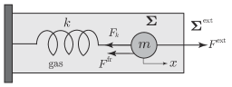
Figure 5.1: A mass-spring-friction system in a room with gas

With the above choice of Lagrangian and force, the general equations (2.4) (arising from the variational formulation (2.1)–(2.3)) yield the time evolution equations of the coupled mechanical and thermal system as

$$m\ddot{x}=-kx-\lambda\dot{x}+F^{\rm ext}(x,\dot{x},S),\qquad\dot{S}=\frac{1}{T}\lambda\dot{x}^{2},$$

where

$$T=\frac{\partial\mathcal{U}}{\partial S}(S)=\frac{\mathcal{U}_{0}}{cN_{0}R}e^{\frac{1}{cRN_{0}}(S-S_{0})}=T_{0}e^{\frac{1}{cRN_{0}}(S-S_{0})}.$$

The total energy, given by $E(x,\dot{x},S)=\frac{1}{2}m\dot{x}^{2}+U(x,S)$, verifies the energy balance equation $\frac{d}{dt}E=\left<F^{\rm ext}(x,\dot{x},S),\dot{x}\right>$.

Exact solutions.

Consider the special case in which there is no external force, i.e., $F^{\rm ext}=0$. In this case the time evolution equations are given by

$$m\ddot{x}=-kx-\lambda\dot{x}\quad\text{and}\quad T\dot{S}=\lambda\dot{x}^{2},$$ (5.5)

and the total energy is preserved. These equations can be easily solved explicitly, see Ferrari and Gruber [2010].

Setting $x_{0}=x(0)$ and $v_{0}=\dot{x}(0)$, the solution of the first equation in (5.5) is

$$x(t)=e^{-\kappa t}\left(x_{0}\cos(\omega t)+\frac{v_{0}+\kappa x_{0}}{\omega}\sin(\omega t)\right),$$ (5.6)

where

$$\kappa=\frac{\lambda}{2m},\;\;\omega_{0}=\sqrt{\frac{k}{m}},\quad\omega=\sqrt{\omega_{0}^{2}-\kappa^{2}},\quad\kappa<\omega_{0}.$$

In order to solve the second equation in (5.5), we note that

$$\frac{d}{dt}\mathcal{U}=T\dot{S}=\lambda\dot{x}^{2}\quad\text{and}\quad\frac{d}{dt}\mathcal{U}=cNR\dot{T},$$ (5.7)

from which we obtain the evolution of the temperature as

$$T(t)=T(0)+\frac{1}{cNR}f(t),\quad\textrm{where $f(t):=\lambda\int_{0}^{t}\dot{x}^{2}(s)ds.$}$$ (5.8)

In the above,

$$\dot{x}(t)=e^{-\kappa t}\left(v_{0}\cos(\omega t)-\left(\kappa\frac{v_{0}+\kappa x_{0}}{\omega}+x_{0}\omega\right)\sin(\omega t)\right)$$

and hence

$$f(t) =\lambda\int_{0}^{t}\dot{x}^{2}(s)$$

$$=\left(\frac{1}{2}mv_{0}^{2}+\frac{1}{2}kx_{0}^{2}\right)-\frac{1}{2(4km-\lambda^{2})}e^{-\frac{\lambda}{m}t}\Big{(}4km(mv_{0}^{2}+\lambda v_{0}x_{0}+kx_{0}^{2})$$

$$\qquad-\lambda(v_{0}^{2}\lambda m+4v_{0}mkx_{0}+\lambda kx_{0}^{2})\cos(2\omega t)-\lambda(mv_{0}^{2}-kx_{0}^{2})(4km-\lambda^{2})^{1/2}\sin(2\omega t)\Big{)}.$$

Using (5.8) and (5.7), we get the explicit evolution of the entropy as

$$S(t)=S(0)+cNR\ln\left(\frac{T(t)}{T(0)}\right).$$ (5.9)

Variational discretizations.

We now apply our variational discretization schemes 1, 2, 3 to this example.

Scheme 1:

The first scheme yields

$$\left\{\begin{array}[]{l}\vspace{0.2cm}\displaystyle m\frac{x_{k+1}-2x_{k}+x_{k-1}}{h^{2}}+kx_{k}=-\lambda\frac{x_{k+1}-x_{k}}{h},\\ \displaystyle\frac{\partial\mathcal{U}}{\partial S}(S_{k})\frac{S_{k+1}-S_{k}}{h}=\lambda\left(\frac{x_{k+1}-x_{k}}{h}\right)^{2}.\end{array}\right.$$

The second equation can be restated as

$$S_{k+1}=\frac{h\lambda}{T_{k}}\left(\displaystyle\frac{x_{k+1}-x_{k}}{h}\right)^{2}+S_{k},\quad$$

where

$$T_{k}=\frac{\partial\mathcal{U}}{\partial S}(S_{k})=\frac{\mathcal{U}_{0}}{cN_{0}R}e^{\frac{1}{cRN_{0}}(S_{k}-S_{0})}=T_{0}e^{\frac{1}{cRN_{0}}(S_{k}-S_{0})}.$$

For this example, the matrix (5.2) of the variational discretization scheme 1 reads

$$\left[\begin{array}[]{cc}-\displaystyle\frac{m}{h}-\lambda&0\\[8.53581pt] 0&\displaystyle\frac{1}{h}T(x_{0},S_{0})\end{array}\right].$$

Thus, since $m>0$, $\lambda\geq 0$, and $T>0$, the discrete flow of the extended Verlet scheme is well-defined.

Scheme 2:

The second scheme yields

$$\left\{\begin{array}[]{l}\vspace{0.2cm}\displaystyle m\frac{x_{k+1}-2x_{k}+x_{k-1}}{h^{2}}+\frac{1}{2}k\left(\frac{x_{k-1}+x_{k}}{2}+\frac{x_{k}+x_{k+1}}{2}\right)\displaystyle=-\frac{1}{2}\lambda\left(\frac{x_{k+1}-x_{k}}{h}+\frac{x_{k}-x_{k-1}}{h}\right),\\[14.22636pt] \displaystyle{\frac{1}{2}}\left[\frac{\partial\mathcal{U}}{\partial S}\left(\frac{S_{k-1}+S_{k}}{2}\right)+\frac{\partial\mathcal{U}}{\partial S}\left(\displaystyle\frac{S_{k}+S_{k+1}}{2}\right)\right]\frac{S_{k+1}-S_{k}}{h}=\lambda\left(\frac{x_{k+1}-x_{k}}{h}\right)^{2}.\end{array}\right.$$

For this example, the matrix (5.3) of the variational discretization scheme 2 reads

$$\left[\begin{array}[]{ll}-\displaystyle\frac{m}{h}-\frac{\lambda}{2}&0\\[8.53581pt] -\displaystyle\frac{2\lambda}{h^{2}}\left(x_{1}-x_{0}\right)&\displaystyle\frac{T}{h}\left(\frac{S_{1}-S_{0}}{2cN_{0}R}+1\right)\end{array}\right],$$

where $T=\frac{\partial\mathcal{U}}{\partial S}\left(\frac{S_{0}+S_{1}}{2}\right)$. Thus, since $m>0$, $\lambda\geq 0$, $T>0$, and $cN_{0}R>0$, the discrete flow of the variational midpoint rule scheme is well-defined.

Scheme 3:

The third example yields

$$\left\{\begin{array}[]{l}\vspace{0.2cm}\displaystyle m\frac{x_{k+1}-2x_{k}+x_{k-1}}{h^{2}}+kx_{k}=-\frac{1}{2}\lambda\left(\frac{x_{k+1}-x_{k}}{h}+\frac{x_{k}-x_{k-1}}{h}\right),\\[5.69054pt] \displaystyle\frac{1}{2}\left[\frac{\partial\mathcal{U}}{\partial S}(S_{k})+\frac{\partial\mathcal{U}}{\partial S}(S_{k+1})\right]\frac{S_{k+1}-S_{k}}{h}=\lambda\left(\frac{x_{k+1}-x_{k}}{h}\right)^{2}.\end{array}\right.$$

For this example, the matrix (5.4) of the variational discretization scheme 3 reads

$$\left[\begin{array}[]{ll}-\displaystyle\frac{m}{h}-\frac{\lambda}{2}&0\\[14.22636pt] -\displaystyle\frac{4\lambda}{h^{2}}\left(x_{1}-x_{0}\right)&\displaystyle\frac{T_{1}}{cN_{0}R}\left(\displaystyle\frac{S_{1}-S_{0}}{h}\right)+(T_{0}+T_{1})\displaystyle\frac{1}{h}\end{array}\right],$$

where $T_{0}=\frac{\partial\mathcal{U}}{\partial S}(S_{0})$ and $T_{1}=\frac{\partial\mathcal{U}}{\partial S}(S_{1})$. Thus, since $m>0$, $\lambda\geq 0$, $T_{1}>0$, $T_{2}>0$ and $cN_{0}R>0$, the discrete flow of the symmetrized Lagrangian variational integrator is well-defined.

5.3 Numerical tests

We illustrate the behavior of the three variational schemes for the mass-spring-friction system, by considering two cases of physical parameters and various values for the friction coefficient, namely $\lambda=0$, $0.2$, $5$, and $10$ ${\rm[N\!\cdot\!s/m]}$.

For each of the five values of $\lambda$ we display the evolutions of the position, entropy, total energy $E(q_{k},q_{k+1},S_{k})$, relative energy errors $\bigr{|}\frac{E(q_{k},q_{k+1},S_{k})-E_{0}}{E_{0}}\bigr{|}$, internal energy, and temperature. Each figure shows the results for the three schemes as well as the exact solution, through $10^{5}$ time steps.

Case 1.

For the first series of numerical tests, we choose the time step $h=10^{-3}{\rm[s]}$ and we set the parameters of the system $\boldsymbol{\Sigma}$ as follows: $m=5\,{\rm[kg]}$, $N=1\,{\rm[mol]}$, $k=5\,{\rm[N/m]}$, $V=2.494\times 10^{-2}\,{\rm[m^{3}]}$. The initial conditions are $x_{0}=0.3\,{\rm[m]}$, $x_{1}=0.3\,{\rm[m]}$, $T_{0}=300\,{\rm[K]}$, $S_{0}=0\,{\rm[J/K]}$.

The results for $\lambda=0$, see Figures 5.2 and 5.3, consistently recover the behavior obtained through a usual variational discretization of the Euler-Lagrange equations for the conservative mass-spring system in classical mechanics. In particular, for each scheme the internal energy $\mathcal{U}(S_{k})=\mathcal{U}_{0}$ is preserved and the temperature, given by $T_{k}=\frac{\partial\mathcal{U}}{\partial S}(S_{k})$, remains a constant, see Figure 5.4. Exactly as in the continuous case, in absence of friction in an isolated simple system, the entropy and temperature stay constant, the system is reversible, and the dynamics is completely described by the Euler-Lagrange equations.

For all the cases with friction, $\lambda=0.2$, $5$, $10$, the numerical solutions of the position, entropy, internal energy, and temperature reproduce the correct behaviors for all the three schemes, as we see from a direct comparison with the exact solutions, see Figures 5.5, 5.7, 5.8, 5.10, 5.11, 5.13.

For Scheme 1, the relative energy error is bounded by $10^{-8}$ for all values of $\lambda$, and decreases in time, whereas for Scheme 2 and 3, the relative energy error is bounded by $10^{-11}$ for all values of $\lambda$, see Figures 5.6, 5.9, 5.12, and stays constant in time.

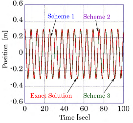
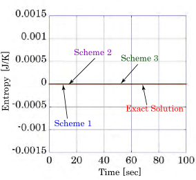
Figure 5.2: Time evolutions of position and entropy (Case 1: $\lambda=0$)

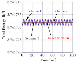
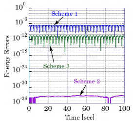
Figure 5.3: Total energy and relative energy error (Case 1: $\lambda=0$)

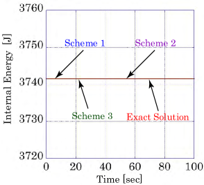
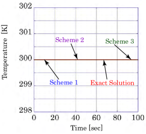
Figure 5.4: Internal energy and temperature (Case 1: $\lambda=0$)

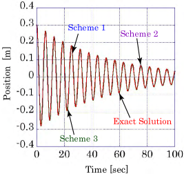
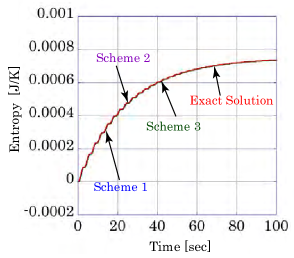
Figure 5.5: Time evolutions of position and entropy (Case 1: $\lambda=0.2$)

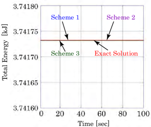
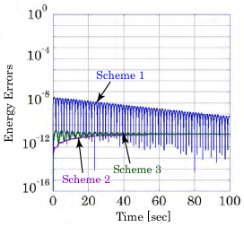
Figure 5.6: Total energy and relative energy error (Case 1: $\lambda=0.2$)

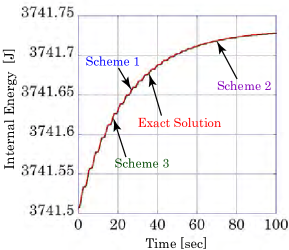
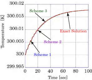
Figure 5.7: Internal energy and temperature (Case 1: $\lambda=0.2$)

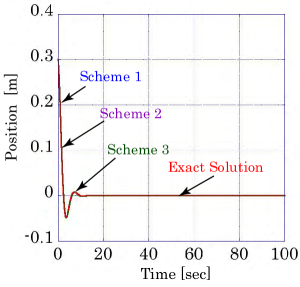
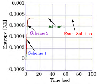
Figure 5.8: Time evolutions of position and entropy (Case 1: $\lambda=5$)

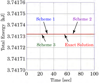
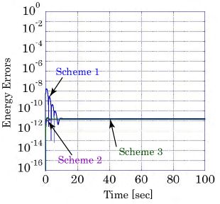
Figure 5.9: Total energy and relative energy error (Case 1: $\lambda=5$)

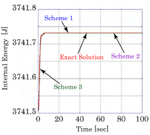
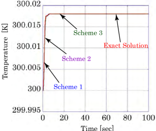
Figure 5.10: Internal energy and temperature (Case 1: $\lambda=5$)

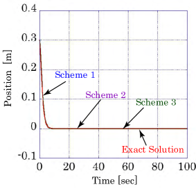
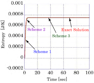
Figure 5.11: Time evolutions of position and entropy (Case 1: $\lambda=10$)

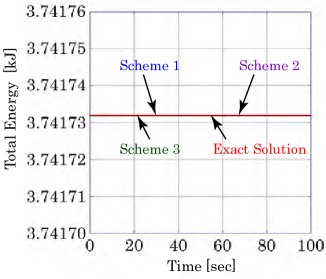
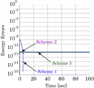
Figure 5.12: Total energy and relative energy error (Case 1: $\lambda=10$)

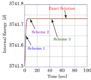
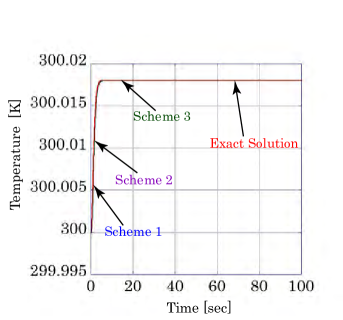
Figure 5.13: Internal energy and temperature (Case 1: $\lambda=10$)

Case 2.

For the second series of numerical tests, we choose the time step $h=10^{-3}{\rm[s]}$ and we set the parameters of the system $\boldsymbol{\Sigma}$ as follows: $m=10\,{\rm[kg]}$, $N=2\,{\rm[mol]}$, $k=20\,{\rm[N/m]}$, $V=9.9775\times 10^{-2}\,{\rm[m^{3}]}$. The initial conditions are $x_{0}=0.1\,{\rm[m]}$, $x_{1}=0.1\,{\rm[m]}$, $T_{0}=300\,{\rm[K]}$, $S_{0}=0\,{\rm[J/K]}$.

The results for $\lambda=0$ are shown in Figures 5.14 and 5.15, and, similarly to Case 1, consistently recover the behavior obtained through a usual variational discretization of the Euler-Lagrange equations. In particular, the internal energy $\mathcal{U}(S_{k})=\mathcal{U}_{0}$ is preserved and the temperature, given by $T_{k}=\frac{\partial\mathcal{U}}{\partial S}(S_{k})$, remains a constant, see Figure 5.16.

For all the cases with friction, $\lambda=0.2$, $5$, $10$, the numerical solutions of the position, entropy, internal energy, and temperature reproduce the correct behaviors for all the three schemes, as we see from a direct comparison with the exact solutions, see Figures 5.17, 5.19, 5.20, 5.22, 5.23, 5.25.

For Scheme 1, the relative energy error is bounded by $10^{-6}$ for all values of $\lambda$, and decreases in time, whereas for Scheme 2 and 3, the relative energy error is bounded by $10^{-9}$ for all values of $\lambda$, see Figures 5.18, 5.21, 5.24, and stays constant in time.

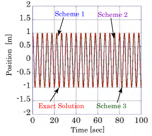
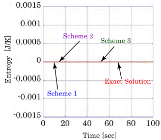
Figure 5.14: Time evolutions of position and entropy (Case 2: $\lambda=0$)

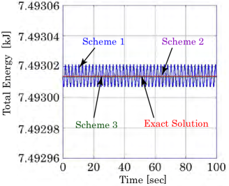
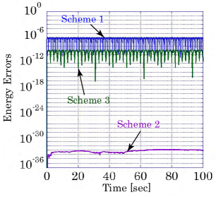
Figure 5.15: Total energy and relative energy error (Case 2: $\lambda=0$)

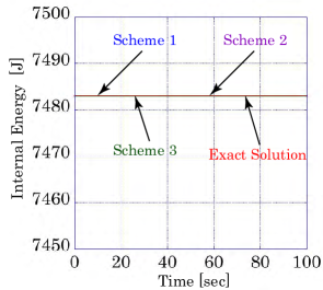
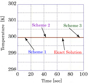
Figure 5.16: Internal energy and temperature (Case 2: $\lambda=0$)

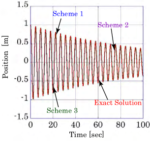
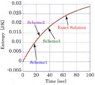
Figure 5.17: Time evolutions of position and entropy (Case 2: $\lambda=0.2$)

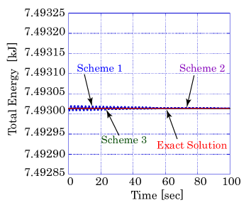
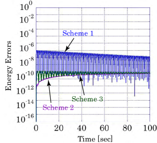
Figure 5.18: Total energy and relative energy error (Case 2: $\lambda=0.2$)

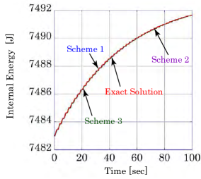
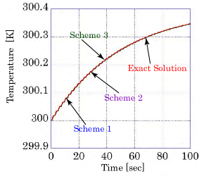
Figure 5.19: Internal energy and temperature (Case 2: $\lambda=0.2$)

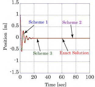
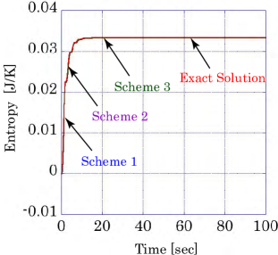
Figure 5.20: Time evolutions of position and entropy (Case 2: $\lambda=5$)

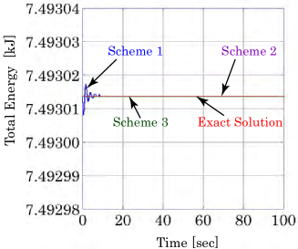
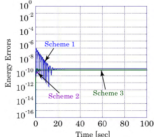
Figure 5.21: Total energy and relative energy error (Case 2: $\lambda=5$)

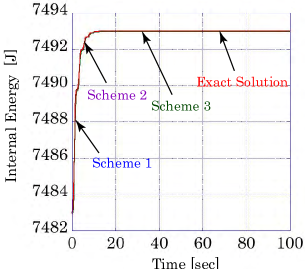
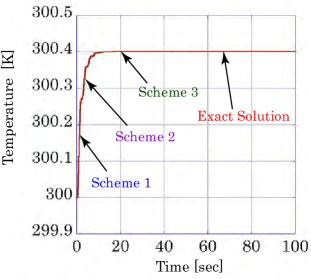
Figure 5.22: Internal energy and temperature (Case 2: $\lambda=5$)

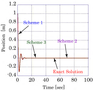
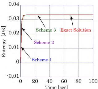
Figure 5.23: Time evolutions of position and entropy (Case 2: $\lambda=10$)

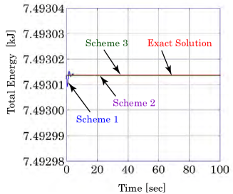
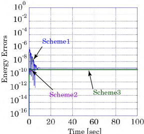
Figure 5.24: Total energy and relative energy error (Case 2: $\lambda=10$)

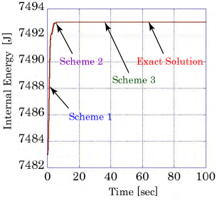
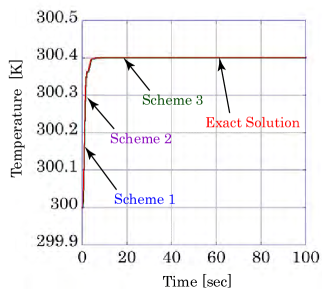
Figure 5.25: Internal energy and temperature (Case 2: $\lambda=10$)

For this particular example of the mass-spring-friction system with thermodynamics, we have observed an excellent total energy behavior for all the three schemes, i.e., changes of mechanical energy are compensated by changes of internal energy during the evolution, exactly as in the continuous case. A thorough study of the energy behaviors of the numerical schemes derived from our variational discretization has to be explored in order to analyze to what class of simple thermodynamical systems does this property extend.

It is important to mention that in general, a variational discretization of the Lagrange-d’Alembert type in mechanics does not necessarily produce a scheme with a well accurate energy behavior. We refer, e.g., to McLachlan and Perlmutter [2006]; Celledoni, et al. [2016] for some examples of such schemes in nonholonomic mechanics which are derived from a discrete Lagrange-d’Alembert principle and which present an energy drift.

Acknowledgements.

The authors thank C. Gruber for extremely helpful discussions and also graduate students, T. Nishiyama and H. Momose, for their supporting in numerical computations. F.G.B. is partially supported by the ANR project GEOMFLUID, ANR-14-CE23-0002-01; H.Y. is partially supported by JSPS Grant-in-Aid for Scientific Research (26400408, 16KT0024), Waseda University (SR 2014B-162, SR 2015B-183), and the MEXT “Top Global University Project”.

References

- Bloch [2003] Bloch, A. M. [2003], Nonholonomic Mechanics and Control, volume 24 of Interdisciplinary Applied Mathematics, Springer-Verlag, New York. With the collaboration of J. Baillieul, P. Crouch and J. Marsden, and with scientific input from P. S. Krishnaprasad, R. M. Murray and D. Zenkov.
- Celledoni, et al. [2016] Celledoni, E., Farré Puiggali, M., Høiseth, E.H., Martin de Diego, D., Energy-preserving integrators applied to nonholonomic systems, https://arxiv.org/pdf/1605.02845v1.pdf
- Cortés and Martínez [2001] Cortés, J. and S. Martínez [2001], Nonholonomic integrators, Nonlinearity 14, 1365–1392.
- Ferrari and Gruber [2010] Ferrari, C. and C. Gruber [2010], Friction force: from mechanics to thermodynamics, Europ. J. Phys. 31(5), 1159–1175.
- Gay-Balmaz [2017] Gay-Balmaz, F. [2017], A variational derivation of the thermodynamics of a moist atmosphere with irreversible processes, https://arxiv.org/pdf/1701.03921v1.pdf
- Gay-Balmaz and Yoshimura [2017a] Gay-Balmaz, F. and H. Yoshimura [2017a], A Lagrangian formulation for nonequilibrium thermodynamics. Part I: discrete systems, J. Geom. Phys., 111, 169–193.
- Gay-Balmaz and Yoshimura [2017b] Gay-Balmaz, F. and H. Yoshimura [2017b], A Lagrangian formulation for nonequilibrium thermodynamics. Part II: continuum systems, J. Geom. Phys., 111, 194–212.
- Green and Naghdi [1991] Green, A. E. and P. M. Naghdi [1991], A re-examination of the basic postulates of thermomechanics, Proc. R. Soc. London. Series A: Mathematical, Physical and Engineering Sciences, 432(1885), 171–194.
- Gruber [1999] Gruber, C. [1999], Thermodynamics of systems with internal adiabatic constraints: time evolution of the adiabatic piston, Eur. J. Phys. 20, 259–266.
- Gruber and Brechet [2011] Gruber, C. and S. D. Brechet [2011], Lagrange equation coupled to a thermal equation: mechanics as a consequence of thermodynamics, Entropy 13, 367–378.
- Hairer, Lubich, and Wanner [2006] Hairer, E., C. Lubich, and G. Wanner [2006], Geometric Numerical Integration, Structure-Preserving Algorithms for Ordinary Differential Equations, Springer Series in Computational Mathematics, 31, Springer, Heidelberg, 2010.
- Kane, Marsden, Ortiz, and West [2000] Kane, C., J. E. Marsden, M. Ortiz, and M. West [2000], Variational integrators and the Newmark algorithm for conservative and dissipative mechanical systems, International Journal for Numerical Methods in Engineering, 49(10), 1295–1325.
- Lew, Marsden, Ortiz and West [2004] Lew, A., J. E. Marsden, M. Ortiz, and M. West [2004a], Variational time integrators, Internat. J. Numer. Methods Eng., 60 (1), 153–212.
- McLachlan and Perlmutter [2006] McLachlan, R. and M. Perlmutter [2006], Integrators for nonholonomic mechanical systems, J. Nonlin. Sci., 16(4), 283–328.
- Moser and Veselov [1991] Moser, J. and A. P. Veselov [1991], Discrete versions of some classical integrable systems and factorization of matrix polynomials, Comm. Math. Phys. 139, 217–243.
- Marsden and West [2001] Marsden, J. E. and M. West [2001], Discrete mechanics and variational integrators, Acta Numer., 10, 357–514.
- Stueckelberg and Scheurer [1974] Stueckelberg, E. C. G. and P. B. Scheurer [1974], Thermocinétique phénoménologique galiléenne, Birkhäuser, 1974.
- Veselov [1988] Veselov, A. P. [1988], Integrable discrete-time systems and difference operators (Russian), Funktsional. Anal. i Prilozhen., 22(2), 1–13, 96; English translation in Funct. Anal. Appl., 22(2), 83–93.
- Veselov [1991] Veselov, A. P. [1991], Integrable Lagrangian correspondences and the factorization of matrix polynomials (Russian), Funkts. Anal. Prilozhen 25(2), 38–49; English translation in Funct. Anal. Appl., 25(2), 112–122.
- von Helmholtz [1884] von Helmholtz, H. [1884], Studien zur Statik monocyklischer Systeme. Sitzungsberichte der Königlich Preussischen Akademie der Wissenschaften zu Berlin, 159–177.
- Wendlandt and Marsden [1997] Wendlandt, J. M. and J. E. Marsden [1997], Mechanical integrators derived from a discrete variational principle, Physica D, 106, 223–246.