Tuning friction with composite hierarchical surfaces

Abstract

Macroscopic friction coefficients observed in experiments are the result of various types of complex multiscale interactions between sliding surfaces. Therefore, there are several ways to modify them depending on the physical phenomena involved. Recently, it has been demonstrated that surface structure, e.g. artificial patterning, can be used to tune frictional properties. In this paper, we show how the global friction coefficients can also be manipulated using composite surfaces with varying roughness or stiffness values, i.e. by combining geometrical features with the modification of local friction coefficients or stiffnesses. We show that a remarkable reduction of static friction can be achieved by introducing hierarchical arrangements of varying local roughness values, or by introducing controlled material stiffness variations.

1 Introduction

The constitutive laws of friction appear to be very simple at the macroscopic scale, indeed they were already formulated by Leonardo da Vinci, and later introduced in the context of classical mechanics with the so called Amonton’s-Coulomb (AC) law: the friction force is proportional to the applied normal load and is independent of the apparent contact surface and of the sliding velocity [1]. The proportionality constants are called friction coefficients, which are different in the static and the dynamic sliding phase. Although some violations have been observed [2], this is a good approximate description of the macroscopic frictional force between two solid sliding surfaces [3].

However, the origin of this behaviour turns out to be much more complicated, since friction coefficients are effective values, enclosing all the interactions occurring from atomic length scales, involving “dry” or chemical adhesion forces, to macroscopic scales, involving forces due to solid deformation and surface roughness. Moreover, friction coefficients are not a specific feature of the specific material, rather they are the result of the complex interplay between the contact surfaces occurring at various length scales in that material and involving different basic physical mechanisms [4][5]. Thus, in order to modify the macroscopic emergent behaviour, one can intervene on the single mechanisms involved. For example, it is possible to modify the interactions at the microscopic level by means of lubrication between surfaces, so that solid-solid molecular forces are switched to liquid-solid interactions and friction is reduced. At the macroscopic level, friction can be reduced by means of smoothing or polishing procedures, in order to remove surface asperities hindering relative motion. Thus, problems related to friction, which is a complex multiscale phenomenon, can be addressed with different methods, from a practical and a theoretical point of view [6].

Another way to modify frictional properties is to manufacture sliding surfaces with artificial patterning, from micrometric to millimetric scales, e.g. grooves and pawls perpendicular to the direction of motion. The effects of these structures have been studied both numerically [7] and experimentally [8][9], and recently their hierarchical arrangement has also been investigated by means of numerical simulations [10]: results show that by changing the architecture of the contact surface only, the global static friction coefficients can be tuned without changing the chemical or physical properties of the material. This is because by exploiting patterning it is possible to modify mesoscopic features, i.e. the effective contact area and the stress concentrations occurring in the static phase, providing a way to modify macroscopic friction coefficients.

In this paper, we show that this approach can be combined with the local variation of friction coefficients, corresponding to a local change of material properties or of local surface roughness, in order to reduce static friction. We consider only roughness modifications occurring at the mesoscopic scale, using a statistical description based on a one-dimensional version of the spring-block model [11]. This approach allows to address the problem of friction in composite materials, which are widely used in practical applications [12]-[16] but whose frictional behavior is still scarcely studied from a theoretical and numerical point of view. Moreover, we consider local hierarchical arrangements of surface properties on different characteristic length scales. This allows us to highlight the main mechanisms taking place in the presence of different length scales, which could be exploited to design artificial surfaces with specific tribologic properties.

Finally, we also consider a composite material with varying elastic properties, i.e. in which the elastic modulus is characterized by a linear grading. This can be found for example in functionally-graded composite materials, i.e. inhomogeneous materials whose physical properties are designed to vary stepwise or continuously [17][18] to manipulate global properties such as elasticity, thermal conductivity, hardness etc. These types of composite materials are widely adopted in practical applications, so that it is useful to investigate their frictional properties. A linear grading of elastic properties can be also combined with a local change of surface roughness in order to exploit both effects.

2 Spring-block model

Figure 1: Schematic of the spring-block model with the notation used in the text.

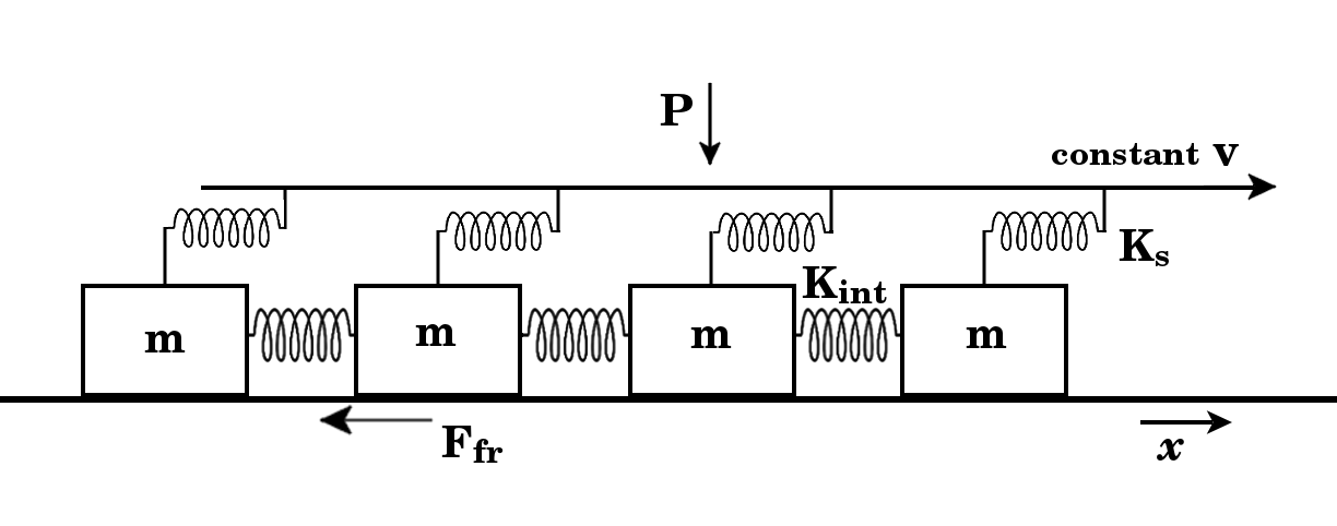
In order to study the effect of varying local friction coefficients on a surface, we adopt the one-dimensional spring-block model [19][20], which is schematically represented in figure 1: the material is discretized in $N$ blocks of mass $m$ along the direction of motion, connected by means of springs of stiffness $K_{int}$ and rest length $l_{x}$. Each block is also attached by means of shear springs of stiffness $K_{s}$ to a slider which is moving at constant velocity $v$. A normal pressure $P$ is applied uniformly to the surface, so that the same normal force is acting on all blocks. A viscous force with damping coefficient $\gamma$ in the underdamped regime is also added, in order to eliminate artificial block oscillations. Despite its simplicity, this model has already been used in many studies to investigate the frictional properties of elastic materials [11],[21]-[30].

The blocks, representing a region of characteristic length $l_{x}$ on the surface of the material, are in contact with an infinitely rigid plane. Friction at the block scale is introduced through the classical AC friction force: each block is characterized by microscopic static and dynamic friction coefficients, respectively ${\mu_{s}}_{i}$, ${\mu_{d}}_{i}$, extracted from a Gaussian statistical distribution. In the following, we will drop the subscripts $s$ or $d$ of the friction coefficients every time the considerations apply to both the coefficients.

This distribution does not necessarily represent the statistics of the contact points due to the surface roughness, rather it is a distribution of force thresholds for an elementary surface unit, used to provide an effective statistical description of the AC friction force at larger length scales than those relative to micro-scale phenomena. Though others can also be appropriate, the Gaussian distribution is a conventional choice that can be used to approximate any peaked distribution with parameters that are easily associated with the mean value and the standard deviation. The probability distribution is $p({\mu}_{i})=(\sqrt{2\pi}\sigma)^{-1}\exp{[-({\mu}_{i}-(\mu)_{m})^{2}/(2\sigma^{2})]}$, where $(\mu)_{m}$ is the average microscopic coefficient and $\sigma$ is its standard deviation. This distribution is adopted for both the coefficients but with different parameters.

The global friction coefficients, obtained from the sum of all the friction forces on the blocks, will be denoted with $M$, i.e. $(\mu)_{M}$. The global dynamic friction coefficient is calculated from the time average during the kinetic phase. The model does not include any roughness variation of value or other long term effects occurring after the onset of macroscopic sliding. Results regarding the dynamic friction are to be intended within the limits of this approximation. The global static friction coefficient is calculated from the maximum of the total friction force during the initial static phase, identified using the absolute maximum of the number of moving blocks, representing a macroscopic sliding event. In most cases, this coincides with the maximum of the total friction force over time.

In summary, the forces acting of each block are: the shear elastic force due to the slider uniform motion, $F_{s}=K_{s}(vt+l_{i}-x_{i})$, where $x_{i}$ is the position of the block $i$ and $l_{i}$ is its starting rest position; the internal elastic restoring force between blocks $F_{int}=K_{int}(x_{i+1}+x_{i-1}-2x_{i})$; the normal force $F_{n}=P\;l_{x}l_{y}$ and the viscous force $F_{d}=-m\gamma\dot{x_{i}}$; finally, the AC friction force $F_{fr}$: if the block $i$ is at rest, the friction force is equal and opposite to the resulting driving force, i.e. $F_{fr}=-(F_{s}+F_{int})$ up to the threshold $F_{fr}={\mu_{s}}_{i}\;{F_{n}}$. When this limit is exceeded, a constant dynamic friction force opposes the motion, i.e. $F_{fr}=-{\mu_{d}}_{i}\;F_{n}$. Thus, the equation of the motion for the block $i$ along the sliding direction $x$ is obtained from Newton’s law: $m\ddot{x}_{i}=F_{int}+F_{s}-m\gamma\dot{x_{i}}+F_{fr}$.

The friction coefficients are fixed at the beginning of the simulation by extracting their values from the chosen distribution with a pseudo-random number generator. We have adopted a generator based on the Mersenne-Twister algorithm [31]. The overall system of ordinary differential equations can be solved numerically with a fourth-order Runge-Kutta algorithm with constant time step integration [32]. Since the friction coefficients of the blocks are assigned after generating them with a pseudo-random number generator from the chosen distribution at each run, the final result of any observable consists on an average of various repetitions of the simulation. Usually, we assume an elementary integration time step $h=10^{-4}$ ms and we repeat the simulation about twenty times for statistical reliability.

The values of the parameters can be assigned by relating them to the macroscopic properties of the material, such as the Young’s modulus $E$, the shear modulus $G$, the mass density $\rho$, the transversal dimensions $l_{y}$, $l_{z}$ and the total length $L_{x}=Nl_{x}$. The mass is $m=\rho\;l_{x}l_{y}l_{z}$, the stiffnesses are $K_{int}=E\cdot(N-1)l_{y}l_{z}/L_{x}$ and $K_{s}=G\cdot l_{y}l_{x}/l_{z}$. The stiffnesses are assumed constant for all the blocks, also in presence of different roughnesses, unless grading is explicitly introduced (see section 6). This choice is made to reduce the number of free parameters of the model, but other formulations are equally valid (e.g. with constant friction coefficients and a statistical dispersion on the stiffnesses) and would not significantly affect the qualitative behaviour. We choose the global shear modulus as $G=5$ MPa, the Young’s modulus $E=15$ MPa, the mass density $\rho=1.2$ g/cm³, which are typical values for a rubber-like material with Poisson ratio $\nu=0.5$.

The length $l_{x}$ is an arbitrary parameter representing the elementary discretization of the material and, consequently, the smallest surface feature that can be described in the model. We have fixed $l_{x}=0.05$ mm, corresponding to a size larger than micro-scale structures, like the surface roughness [33][34] or microscopic patterns [35]-[37]. In any case, qualitative results are not affected by changing this parameter by an order of magnitude. The transversal lengths are fixed to $l_{z}=0.05$ mm, $l_{y}=1.0$ mm. The damping coefficient $\gamma$ is an arbitrary parameter which is tuned in the underdamped regime so that it is smaller than the characteristic frequencies of the system [24]. We fix $\gamma=100$ ms^-1, $N=480$, $v=0.05$ cm/s, $P=0.1$ MPa. The microscopic friction coefficients are specified for each considered case.

3 Friction on uniform surfaces

The spring-block model described in section 2 requires that microscopic friction coefficients be assigned to each block, extracting them from a statistical distribution, while the global friction coefficients are deduced by solving the equation of motion of the whole system. In this section, we investigate how the global friction coefficients are affected by these microscopic distributions of the friction coefficients, while other parameters are unchanged from section 2. This is useful to derive the behaviour of the model as a benchmark for the next sections, where more complex statistical distributions are introduced for the blocks. Here and in the next sections we will focus on the static friction coefficient, since the dynamic one has already been studied in [10].

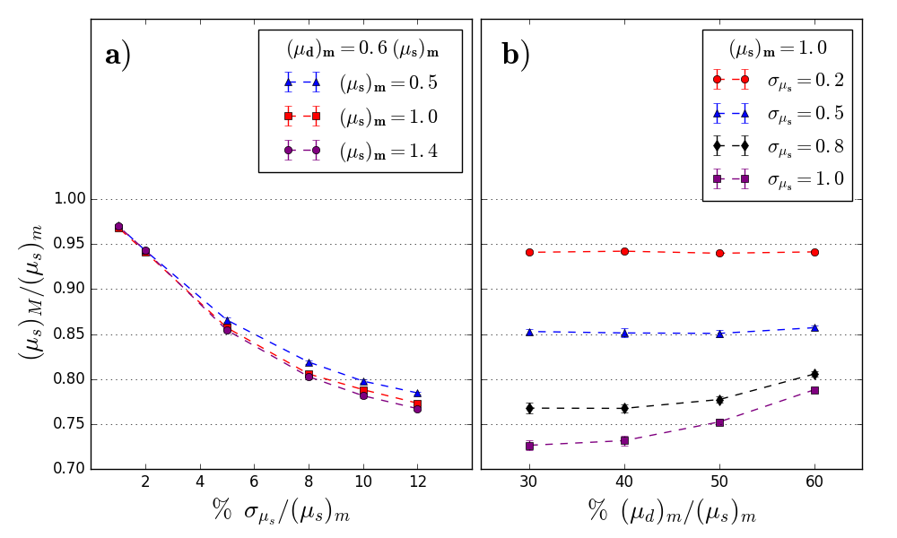
In general, the numerical simulation of static friction is similar to that in a fracture mechanics problem [38]. The static friction coefficient distribution, corresponding to the threshold forces for block motion, are analogous to the thresholds for breaking bonds in fiber bundle or lattice spring models [39][40]. Hence, we expect the global friction coefficient to decrease with a wider static statistical distribution, since the presence of weaker elements can trigger avalanche ruptures leading to a macroscopic sliding event. This is confirmed by numerical simulations in figure 2a: for narrow statistical distributions, the relative reduction from $(\mu_{s})_{m}$ to $(\mu_{s})_{M}$ depends only on the ratio between microscopic static and dynamic coefficients. For a larger variance this is correct only as first approximation. This behaviour is taken as a reference for the cases considered in the following, when variations of the local coefficient distributions are introduced along then surface to model a spatially varying surface roughness. Figure 2b shows that the local dynamic coefficient influences the global static coefficient only for large variance values of the local static coefficients. This is because the macroscopic detachment phase (i.e. when some blocks are already in motion while others are still attached to the substrate) is longer with larger variances, so that the dynamic friction forces due to the moving blocks influence the total friction.

Figure 2: a) Global static friction coefficients $(\mu_{s})_{M}$ as a function of the statistical dispersion of the local ones $\sigma_{\mu_{s}}$ (with a fixed ratio between microscopic dynamic and static values $(\mu_{d})_{m}$ and $(\mu_{s})_{m}$, respectively). At first order the results do not depend on the values of the local static coefficients. b) Global static coefficients as a function the local dynamic coefficient (with a fixed local static one). For small variance values, the global static coefficient becomes insensitive to the local dynamic coefficient value.

4 Friction on variable-roughness patterned surfaces

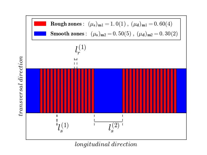
For the sake of simplicity, let us assume that our system can display two types of surface roughnesses (figure 3): for simplicity we will call them “rough” and “smooth” regions, although both have non negligible friction. In the rough regions of the surface the local friction coefficients are extracted from a probability distribution with $(\mu_{s})_{m1}=1.0(1)$ and $(\mu_{d})_{m1}=0.60(4)$, while in the smooth ones $(\mu_{s})_{m2}=0.50(5)$ and $(\mu_{d})_{m2}=0.30(2)$. The global friction coefficients for a uniform surface with these coefficients are $(\mu_{s})_{M1}=0.788(2)$, $(\mu_{d})_{M1}=0.616(4)$ for rough regions, and $(\mu_{s})_{M2}=0.398(2)$, $(\mu_{d})_{M2}=308(3)$ for smooth ones. As expected from section 3, their ratio is about one half.

Let us consider pattern of alternating rough and smooth regions with a characteristic length $l_{g}$, as depicted in figure 3. All other parameters of the system are fixed. In this configuration half of the surface is rough, and half is smooth. The number of blocks in a length $l_{g}$ is indicated as $n_{g}$, so that $l_{g}=n_{g}l_{x}$. Thus, the number of blocks in a rough zone $n_{r}$ or a smooth one $n_{s}$ are $n_{r}=n_{s}=N/(2n_{g})$.

Figure 3: Example of a pattern alternating rough and smooth zones of length $l_{g}$, with local friction coefficients respectively $(\mu)_{m1}$, $(\mu)_{m2}$.

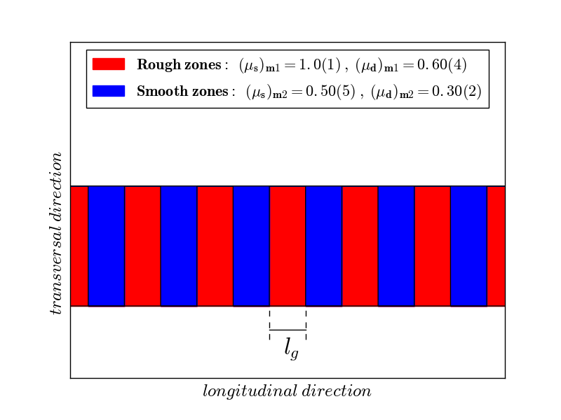
The structure considered in figure 3 is similar to a patterned surface with grooves, in which the friction coefficient is assumed to be zero. In this case, it is known both from numerical studies [7] and experimental results [41][42] that static friction decreases with the width of the grooves. In our previous work [10] we have also shown that this is due to the increase of the shear stress concentrations at the edge of the grooves. In the present situation, instead, the whole surface is in contact with the rigid substrate, but the mean value of the static friction coefficient varies periodically along the slider.

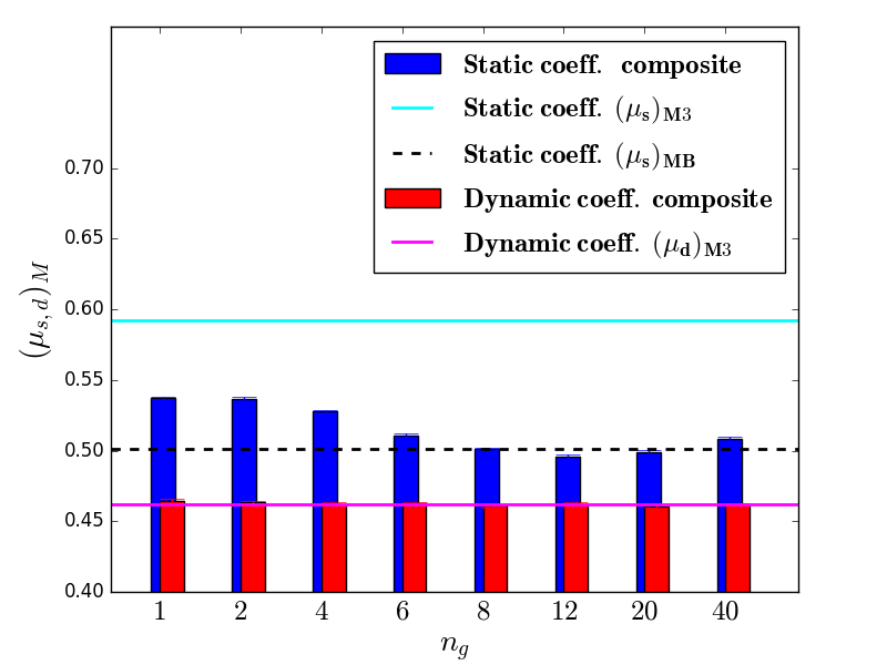
In this case, the resulting global coefficient is expected to be included between the mean values of the two areas: $(\mu)_{M2}<{\mu}_{M}<(\mu)_{M1}$. In particular one could trivially think that the result for the global coefficient should be close to that obtained by setting as microscopic average $(\mu)_{m3}=((\mu)_{m1}+(\mu)_{m2})/2$, i.e. the arithmetic mean between the microscopic coefficients of the rough and smooth zones. Instead, as shown in figure 4, this is true only for the dynamic coefficient, while the static one always displays a reduction with respect to the average value. In particular, if we extract the microscopic coefficients of the blocks from a single Gaussian distribution corresponding to the arithmetic mean, $(\mu_{s})_{m3}=0.75(7)$ and $(\mu_{d})_{m3}=0.45(3)$, we obtain $(\mu_{s})_{M3}=0.592(3)$ and $(\mu_{d})_{M3}=0.462(1)$, while the coefficients obtained with a pattern of rough and smooth zones are always smaller. These results are consistent with those obtained with a multiscale version of the model, whose implementation is conceptually different, but applied to the same structure [43].

This effect is due to the different variance between a single Gaussian distribution for all the surface and two separate Gaussian distributions: although the mean value is the same, the global static coefficient is reduced when a wider statistical dispersion is present, as shown in section 3. If we extract all the local coefficients from a bimodal Gaussian distribution (i.e. double peaked around $(\mu)_{m1}$ and $(\mu)_{m2}$), the result is $(\mu_{s})_{MB}=0.501(2)$, i.e. twenty percent less than that of a single Gaussian. This configuration corresponds to a random arrangement of rough and smooth regions, as could be realized by a composite material, whose two component materials have different statistically distributed frictional properties.

The resulting global friction properties are not dependent on statistical effects, since there is also an influence due to geometry: as shown in figure 4, the size $l_{g}$ of the regions influences the global static coefficient similarly to what is observed with a patterning of grooves and pawls. The fundamental difference is that, in the present case, all blocks are always in contact, and the normal load is equally distributed along the whole surface, but a similar mechanism takes place: when the contact points of the surface in the smooth zones (typically with smaller threshold forces) begin to slide, they lead to an increase in the force exerted on the points still at rest in the rough zones, so that static friction is reduced with respect to $(\mu_{s})_{M3}$ for any $l_{g}$. Moreover, the resulting global static coefficient can be either be tuned to be greater or smaller than $(\mu_{s})_{MB}$, depending on the length $l_{g}$.

This example shows how the geometric organization of rough and smooth zones along the surface allows to modify static friction. In the following, we show that by combining this idea with a hierarchical structure, it is possible to obtain an even more consistent static friction reduction.

Figure 4: Global friction coefficients as a function of the ratio between the widths of rough and smooth zones $n_{g}=l_{g}/l_{x}$. For comparison, we also show the global friction coefficients of a uniform surface, whose microscopic coefficients are extracted from a single Gaussian distribution with mean value corresponding to the arithmetic mean of the rough and smooth zones (the continuous lines, indicated with $(\mu)_{M3}$ in the text). The dotted line indicates the static coefficient $(\mu_{s})_{MB}$ obtained with a bimodal Gaussian distribution.

5 Friction on surfaces with hierarchically patterned roughness

In this section, we investigate the effects on global friction coefficients induced by hierarchical organization of the regions with different roughnesses, as shown for example in figure 5. This configuration is hierarchical in the sense that there are two different length scales for the smooth regions (blue in the figure), that are included between the rough ones (red in the figure). To compare the results with those of section 4, we choose a hierarchical pattern in which half of the overall surface area is smooth and the other is rough, so that the mean value of the distributions of the microscopic coefficients is still $(\mu)_{m3}$.

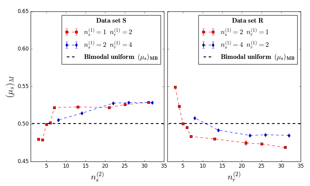
We identify such configurations by indicating the length of the smooth zones and the rough ones, respectively $l_{s}^{(i)}$ and $l_{r}^{(i)}$, ordered with the index $i$ increasing for the larger length scale. For example, the configuration shown in figure 5 is characterized by the parameters $l_{s}^{(1)}$, $l_{s}^{(2)}$ and $l_{r}^{(1)}$, i.e. there are large smooth zones of size $l_{s}^{(2)}$, and then smaller rough and smooth zones of sizes $l_{r}^{(1)}$ and $l_{r}^{(1)}$, respectively. We can express these quantities using the adimensional ratios $n_{s}^{(i)}\equiv l_{s}^{(i)}/l_{x}$ and $n_{r}^{(i)}\equiv l_{s}^{(i)}/l_{x}$, representing the number of blocks for each region. Results for these configurations are shown in figure 6.

Figure 5: Example of a surface with a hierarchical arrangement of smooth zones alternating with rough ones. The ratio between the sizes indicated in the figure are $l_{s}^{(2)}/l_{s}^{(1)}=33$, $l_{r}^{(1)}/l_{s}^{(1)}=3$, where the subscript $s$ denotes the smooth zones and $r$ the rough ones. The pattern is designed in such way that exactly half of the total surface is covered by rough zones and the other half by smooth zones.

A complementary configuration to that shown in figure 5 can be obtained by exchanging the rough regions with the smooth ones, i.e. the subscript $s$ with $r$. In this case the statistics of the detachment thresholds for the configuration are exactly the same, but the geometry is different. In the case of a single level of patterning, as in section 4, there is no effect by exchanging rough and smooth zones, while with a hierarchical arrangement the results are not symmetric and differ by up to ten percent. Since the statistics is the same, this effect is purely geometric. Thus, we have found a peculiar feature which can be obtained by means of hierarchical structures. We will call “data set S” that obtained with two length scales for the smooth regions (exactly as in figure 5) and “data set R” the complementary one, i.e. with two length scales for rough regions.

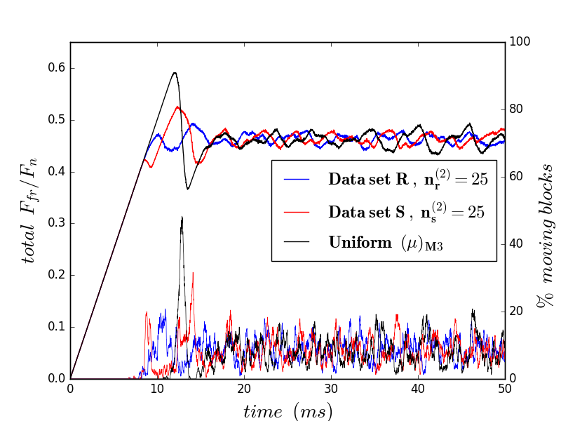
As we can see in figure 6, there are two different regimes leading to an increase or a decrease of the static friction with respect to the case of a uniform surface with local coefficients extracted from the bimodal Gaussian distribution: for data set S, static friction is greater for larger separations between length scales, i.e. for a large asymmetry between rough and smooth regions. Hence, configurations similar to data set R are preferable to reduce static friction and to “flatten” the transition between the static and kinetic phase. This is because of the interplay between microscopic degrees of freedom during the transition from static to kinetic friction, as shown in figure 7, where the total friction force as a function of time is compared for both the data sets.

Thus, it is possible to tune the static friction by means of a hierarchical organization of zones with different roughnesses, and to obtain a friction coefficient close to the lower nominal limit $(\mu)_{M2}$, but with only half of the surface smoothed. From this we can conclude that to reduce the static friction of a material it is sufficient to smooth only part of the surface as long as it is in a “smart” way.

Figure 6: Global static friction coefficients for hierarchical configurations such as the one shown in figure 5, as a function of the larger length scale, that is $n_{s}^{(2)}$ for data set S and $n_{r}^{(2)}$ for data set R. The smaller length scales are reported in the legends. The dashed line indicates the case of a uniform surface with local friction coefficients $(\mu)_{MB}$ extracted from the bimodal Gaussian distribution.

Figure 7: Comparison of the total normalized friction force, as a function of time, between the data set S (case $n_{s}^{(1)}=2$, $n_{r}^{(1)}=1$, $n_{s}^{(2)}=25$ ), data set R (case $n_{r}^{(1)}=2$, $n_{s}^{(1)}=1$, $n_{r}^{(2)}=25$ ) and the uniform case with the same arithmetic mean of the local friction coefficient. The difference in the structure of the local friction coefficients of the illustrated cases causes a different qualitative transition between the static and dynamic sliding phase. On the right, axis the time evolution of the number of moving blocks is reported.

6 Friction on surfaces with graded stiffness

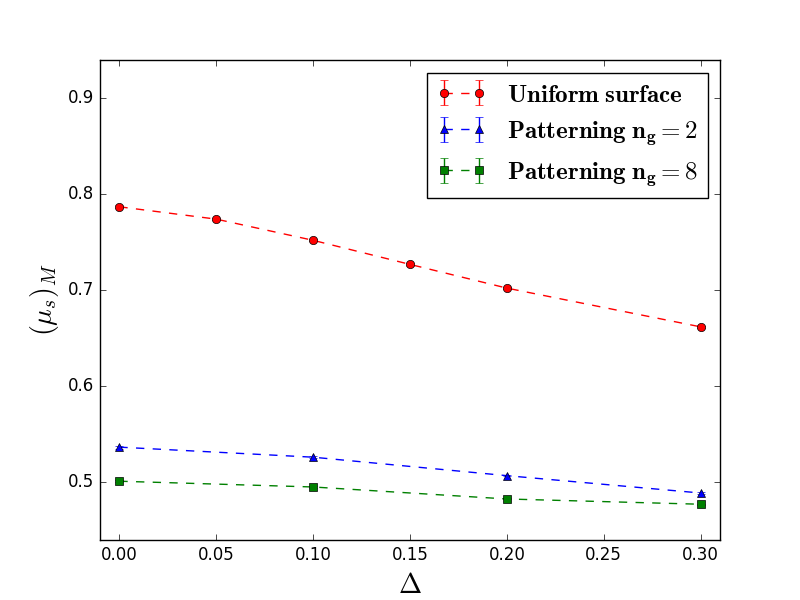
In this section, we investigate the modification of static friction due to the introduction of a linear grading of the elastic modulus, as occurs in a functionally graded composite material. We consider a linear increase (or decrease) of the elastic modulus along the longitudinal direction of the material, i.e. the sliding direction. In the spring-block model, this means that $K_{int}$ and $K_{s}$ depend on the block index $i$. In order to compare the results, the overall stiffness value $(K_{s})_{tot}\equiv\sum_{i}(K_{s})_{i}$ is fixed, and similarly for $K_{int}$. Then, we introduce the relative maximum variation at the edges, namely $\Delta$, so that $\Delta=0.2$ means, for example, that for both the stiffnesses the maximum difference at the edge is twenty percent above/below their average. In symbols, $(K_{s})_{i}=K_{s}(1+\Delta(2i/(N-1)-1))$ where $K_{s}$ is the value without grading, and the same holds for $K_{int}$.

In the spring-block model, variations of $K_{int}$ turn out to be irrelevant, so that the effect can be studied by setting the grading only on the springs $K_{s}$. Results are shown in figure 8. In the presence of grading, the static friction coefficient is considerably reduced. The explanation for this is that in this case the local rupture/sliding thresholds are exceeded sooner than in the case with no grading in the region where the stiffnesses are increased, so that an avalanche of ruptures is triggered in the neighbouring contact points, until the whole surface detaches. We observe no dependence on the orientation of the grading. Also the dynamic friction coefficient is left unchanged.

The exact amount of change of the static friction depends on the system parameters, but we may expect this effect on every configuration, because the grading always induces a stress distribution on the surface that favors avalanche phenomena. Indeed, a reduction of the static friction is also observed in the case of patterning of the local surface roughness. In these simulations, only a linear grading has been considered, but similar effects are expected with a generic functional shape. Thus, we have shown that a further reduction of the static friction can be obtained with a grading on the elastic properties of the material, i.e. in a composite material with a functionally-graded elastic modulus.

Figure 8: Decrease of the macroscopic static friction coefficient as a function of the elastic modulus grading level for a uniform surface with microscopic coefficients $(\mu)_{m1}$ (red points), and for two cases of periodic patterning of the local roughness, as in section 4, with $n_{g}=2$ (blue points) and $n_{g}=8$ (green points).

7 Conclusions

In this paper, we have investigated by means of numerical simulations the variation of the friction coefficients of a material characterized by two distinct surface roughnesses and local friction coefficients, as found in composite materials, or in materials whose surfaces have different degrees of smoothing. For this purpose, we have adopted a one-dimensional version of the spring-block model, which is particularly appropriate for parametric studies on the frictional behaviour of a structured elastic material.

First, we have studied the effects due to statistical variations in surface roughness of a composite surface: the presence of a double-peaked distribution of the local friction coefficients implies that the variance is typically larger than for a single peak distribution, so that static friction is reduced. This effect also occurs without any surface patterning.

Secondly, we have evaluated the influence of the geometry on these composite systems. If the surface is divided into rough and smooth regions of the same size, the global static friction coefficient depends on their length scale, similarly to the case of a surface with a patterning of grooves and pawls. This effect is purely due to structure, since the statistics is the same, and the patterning can be used either to reduce the static friction or to increase it depending on the length scale of the different roughness zones. Thus, in order to considerably reduce static friction, it is sufficient to smooth only a part surface, as long as this is done in a “smart” way.

If instead we introduce different length scales for rough and smooth regions, i.e. we adopt a hierarchical organization of the zones with different roughnesses, we obtain opposite results depending on the ordering between rough and smooth zones. The surface is no longer symmetric under the exchange of the smooth and rough zones, and this has an influence on the global frictional behaviour. Thus, the geometric and multiscale arrangement is crucial to determine measurable variations of static friction, even when the statistical properties of the local coefficients are the same. This example suggests a possible mechanism for modifying the static friction properties of a surface by combining different mesoscopic roughness and geometric parameters. Additionally, it is possible to modify not only the numerical value of the static coefficient, but also the qualitative behaviour of the transition from static to dynamic friction.

Finally, we have considered a composite material with a graded elastic modulus by considering linearly varying stiffnesses in the spring-block model. Results show that this provides the possibility of a further reduction of the static friction, both in the case of a smooth surface and of patterning of the local roughness.

All of these results can be relevant for a large number of applications where maximization or minimization of friction is crucial. One example could be the friction performance of vehicle tires that are typically produced in reinforced rubber composites with various levels of patterning or roughnesses. The large level of tunability of properties obtained exploiting composite material composition, stiffness, roughness and patterning provide an attractive way to reach desired properties, and the presented model a useful tool in the design of optimal solutions.

References

- [1] B.N.J. Persson, Sliding Friction - Physical principles and application, in Nanoscience and Technology, Springer-Verlag Berlin Heidelberg (2000)
- [2] Y. Katano, K. Nakano, M. Otsuki, H. Matsukawa, Novel Friction Law for the Static Friction Force based on Local Precursor Slipping, Sci. Rep. 4 (2014) 6324
- [3] V. Popov, Contact Mechanics and Friction, Springer-Verlag Berlin Heidelberg (2010)
- [4] M. Nosonovsky, B. Bhushan, Multiscale friction mechanisms and hierarchical surfaces in nano- and bio-tribology, Mater. Sci. Eng. R 58 (2007) 162
- [5] B. Bhushan, Introduction to Tribology, 2nd Edition Wiley (2013)
- [6] A. Vanossi, N. Manini, M. Urbakh, S. Zapperi, E. Tosatti, Colloquium: Modeling friction: From nanoscale to mesoscale, Rev. Mod. Phys. 85 (2013) 529
- [7] R. Capozza, N.M. Pugno, Effect of Surface Grooves on the Static Friction of an Elastic Slider, Tribol. Lett. 58 (2015) 35
- [8] M.J. Baum, L. Heepe, E. Fadeeva, S.N. Gorb, Dry friction of microstructured polymer surfaces inspired by snake skin, Beilstein J. Nanotechnol. 5 (2014) 1091
- [9] S. Maegawaa, F. Itoigawa, T. Nakamura, Effect of surface grooves on kinetic friction of a rubber slider, Tribology International, 102 (2016) 326
- [10] G. Costagliola, F. Bosia, N.M. Pugno, Static and dynamic friction of hierarchical surfaces, Phys. Rev. E 94 (2016) 063003
- [11] O.M. Braun, I. Barel, M. Urbakh, Dynamics of Transition from Static to Kinetic Friction, Phys. Rev. Lett. 103 (2009) 194301
- [12] K. Friedrich editor, Advances in composite tribology, Composite materials series, vol. 8, Elsevier, Amsterdam (1993)
- [13] J.W. Hutchinson, H.M. Jensen, Models of fiber debonding and pullout in brittle composites with friction, Mechanics of materials, 9 (1990) 2
- [14] Z.P. Lu, K. Friedrich, On sliding friction and wear of PEEK and its composites, Wear 181 (1995) 624
- [15] S.J. Kim, H. Jang, Friction and wear of friction materials containing two different phenolic resins reinforced with aramid pulp, Tribology International 33 (2000) 7
- [16] B.K. Satapathy, J. Bijwe, Composite friction materials based on organic fibres: Sensitivity of friction and wear to operating variables, Composites A 37 (2006) 1557
- [17] S. Suresh, Graded Materials for Resistance to Contact Deformation and Damage, Science 292 (2001) 2447
- [18] G. Udupa, S.Shrikantha Rao, K.V. Gangadharan, Functionally graded composite materials: an overwiev, Procedia Materials Science 5 (2014) 1291
- [19] R. Burridge and L. Knopoff, Model and theoretical seismicity, Bull. Seismol. Soc. Am. 57 (1967) 341
- [20] S.R. Brown, C.H. Scholz, J.B. Rundle, A simplified spring-block model of earthquakes, Geophys. Res. Lett. 18 (1991) 2
- [21] S. Maegawa, A. Suzuki, K. Nakano, Precursors of Global Slip in a Longitudinal Line Contact Under Non-Uniform Normal Loading, Tribol. Lett. 38 (2010) 3
- [22] J. Scheibert, D.K. Dysthe, Role of friction-induced torque in stick-slip motion, EPL 92 (2010) 5
- [23] R. Capozza, S.M. Rubinstein, I. Barel, M. Urbakh, J. Fineberg, Stabilizing Stick-Slip Friction, Phys. Rev. Lett. 107 (2011) 024301
- [24] J. Trømborg, J. Scheibert, D.S. Amundsen, K. Thøgersen, A. Malthe-Sørenssen, Transition from Static to Kinetic Friction: Insights from a 2D Model, Phys. Rev. Lett. 107 (2011) 074301
- [25] E. Bouchbinder, E.A. Brener, I. Barel, M. Urbakh, Slow Cracklike Dynamics at the Onset of Frictional Sliding, Phys. Rev. Lett. 107 (2011) 235501
- [26] D. S. Amundsen, J. Scheibert, K. Thøgersen, J. Trømborg, A. Malthe-Sørenssen, 1D Model of Precursors to Frictional Stick-Slip Motion Allowing for Robust Comparison with Experiments, Tribology Letters 45 (2012) 357
- [27] J. Trømborg, H.A. Sveinsson, K. Thøgersen, J. Scheibert, A. Malthe-Sørenssen, Speed of fast and slow rupture fronts along frictional interfaces Phys. Rev. E 92 (2015) 012408
- [28] D. S. Amundsen, J. Trømborg, K. Thøgersen, E. Katzav, A. Malthe-Sørenssen, J. Scheibert, Steady-state propagation speed of rupture fronts along one-dimensional frictional interfaces, Phys. Rev. E 92 (2015) 032406
- [29] R. Capozza and M. Urbakh, Static friction and the dynamics of interfacial rupture, Phys. Rev. B 86 (2012) 085430
- [30] N.M. Pugno, Q. Yin, X. Shi, R. Capozza, A generalization of the Coulomb’s friction law: from graphene to macroscale, Meccanica 48 (2013) 8
- [31] E. Gentle, Random Number Generation and Monte Carlo Methods (Statistics and Computing). Springer-Verlag, New York (2003)
- [32] J. Butcher, Numerical Methods for Ordinary Differential Equations, Second Edition, John Wiley & Sons, Ltd, Chichester (2008)
- [33] B.N.J. Persson, O.Albohr, U.Tartaglino, A.I. Volokitin, E. Tosatti, On the nature of surface roughness with application to contact mechanics, sealing, rubber friction and adhesion, J. Phys. Condens. Matter 17 (2005) R1
- [34] M.J. Baum, A.E. Kovalev, J. Michels, S.N. Gorb, Anisotropic Friction of the Ventral Scales in the Snake Lampropeltis getula californiae, Tribol Lett 54 (2014) 139
- [35] B. Murarash, Y. Itovicha, M. Varenberg, Tuning elastomer friction by hexagonal surface patterning, Soft Matters 7 (2011) 5553
- [36] H. E. Jeong, J.K. Lee, H.N. Kim, S.H. Moon, K.Y. Suh, A nontransferring dry adhesive with hierarchical polymer nanohairs, Proc. Nat. Acad. Sci. USA, 106, 14 (2009) 5639
- [37] J. Lee, B. Bush, R. Maboudian, R. Fearing, Gecko-inspired combined lamellar and nanofibrillar array for adhesion on nonplanar surface, Langmuir, 25, 21 (2009) 449
- [38] E. Bayart, I. Svetlizky, J. Fineberg, Fracture mechanics determine the lengths of interface ruptures that mediate frictional motion, Nature Physics 12 (2016) 166
- [39] N.M Pugno, F. Bosia, A. Carpinteri, Multiscale stochastic simulations for tensile testing of nanotube-based macroscopic cables, Small 4 (2008) 8
- [40] L. Brely, F. Bosia, N.M. Pugno, A hierarchical lattice spring model to simulate the mechanics of 2-D materials-based composites, Frontiers in Materials 2 (2015) 51
- [41] E. Gualtieri, A. Borghi, L. Calabri, N.M. Pugno, S. Valeri, Increasing nanohardness and reducing friction of nitride steel by laser surface texturing, Tribol. Int. 42 (2009) 699
- [42] R. Capozza, A. Fasolino, M. Ferrario, A. Vanossi, Lubricated friction on nanopatterned surfaces via molecular dynamics simulations, Phys. Rev. B 77 (2008) 235432
- [43] G. Costagliola, F. Bosia, N.M. Pugno, Hierarchical spring-block model for multiscale friction problems, ACS Biomater. Sci. Eng. doi:10.1021/acsbiomaterials.6b00709