Understanding the Spatial and Temporal Activity Patterns of Subway Mobility Flows

Zhanwei Du Department of Computer Science, Hong Kong Baptist University, Kowloon Tong KLN, Hong Kong Bo Yang School of Computer Science and Technology, Jilin University, Changchun, China Jiming Liu

Abstract

In urban transportation systems, mobility flows in the subway system reflect the spatial and temporal dynamics of working days. To investigate the variability of mobility flows, we analyse the spatial community through a series of snapshots of subway stations over sequential periods. Using Shanghai as a case study, we find that the spatial community snapshots reveal dynamic passenger activities. Adopting a dual-perspective, we apply spatial and temporal models separately to explore where and when individuals travel for entertainment. In the two models, microblog topics and spatial facilities such as food venues and entertainment businesses are used to characterise the spatial popularity of each station and people’s travelling perceptions. In the studied case, the city centre is characterised by greater social influence, and it is better described by the spatial model. In the temporal model, shorter travel distances motivate individuals to start their trips earlier. Interestingly, as the number of food-related facilities near the starting station increases, until it exceeds 1563, the speed of people’s journeys slows down. This study provides a method for modelling the effects of social features on mobility flows and for predicting the spatial-temporal mobility flows of newly built subway stations.

Introduction

Urban transport plays an important role in shaping and reflecting the evolution of cities [1, 2]. To create the desired social-economic outputs, urban transport planners use human mobility flows to understand the spatial-temporal interactions of people [1] on transportation systems. An urban public transport network (UTN) consists of the mobility flows of an urban transportation system, where the nodes represent the public transit stand locations and the directional edges denote the mobility flows from one node to another [3]. For example, in a subway network, each node denotes a subway station and each edge denotes the mobility flow between two nodes, weighted by the volume.

The mobility flows dynamically change over time as people’s reasons for travelling change activities (e.g. work or entertainment) [4]. To measure the variability of spatial-temporal mobility flows, communities in a UTN (a community is a set of densely interconnected nodes that have few connections to outside nodes [5]) are used to show the dynamic changes in UTN over time. Furthermore, a community snapshot is a snapshot of the communities in a UTN at a single point in time (e.g. a period, day or year). Community snapshots have many applications in transport planning, e.g. in urban development analysis, experts use them to quantify the influence of urban development on transportation networks [6, 7]; in urban dynamics analysis, experts use them to measure the variability of human mobility patterns [4]; and in urban area analysis, experts use them to identify functional zones [8]. The community method is not the only means of observing dynamic mobility flows; driven spatial-temporal models with high-order structures of activity patterns are also valuable in many scenarios. For example, in public transit scheduling and pricing, ticket prices are optimised to ease traffic congestion by influencing passengers’ driven models of temporal scheduling [9]; in urban planning, cities can be planned according to valuable factors, i.e. factors that attract individuals’ decisions to live in a or visit a particular place [10]. To further understand the dynamic decision-making processes that shape individuals’ spatial-temporal movements, we study dynamic mobility flows by measuring the variability in a heterogeneous sample of community snapshots in a UTN and explore the models that drive these patterns.

We observe the dynamic mobility flows using community snapshots of different spatial stations over time. These flows exist in many public transit systems (e.g. shared bicycle systems [11, 12], public bus systems [13, 14] and taxi systems [15, 16]). Here, we use a subway system, an important part of a public transport network [3], to demonstrate the use of community snapshots. As current static or aggregated mobility measures are robust to perturbations and cannot clearly reveal the variability of temporal community structures [4], communities patterns are commonly studied retrospectively to get a deeper understanding of how people’s activities change over time. Here, we study changes in the use of a subway system by detecting and comparing community snapshots from different time periods [4, 6]. Retrospective studies of community snapshots improve our ability to measure the mobility flows from the perspective of the network. However, they do not provide insight into the spatial-temporal models that drive the mobility dynamics. For the current day, we cannot determine where individuals would like to go, let alone when they would like to begin any of their activities.

To address this issue, we also study the patterns of passengers’ movements between places [17, 18, 19, 20] as a high-order spatial-temporal structure. The examination of the activity patterns should answer two questions: (1) where do individuals travel to for their activities; and (2) when do people start their activities? For example, in the evening, can our models infer where and when a person is likely to go for entertainment after work? These studies will raise planners’ awareness of human movements between stations over different time periods. Specifically, the likelihood of an individual participating in an activity in a particular spatial-temporal space is associated with both the station’s spatial characteristics (such as population density and number of retail venues) and temporal characteristics (such as the day of the week and time of day) [17].

Previous studies of the where (spatial) dimension of intra-urban spatial mobility in public transit have typically focused on regional populations (such as Beijing [21, 22], Shenzhen [22], London [21], Chicago [21, 22], Los Angeles [21] and Abidjan [22]) and travelling distance (e.g. in Seoul [23]). However, the correlation between public transit and its surrounding economic and social environment is obvious (such as in Biscay [24]), especially the subway system (e.g. in Sao Paulo[25]). Most of the existing studies focus on universal laws of human intra-urban mobility, but neglect the influence of a heterogeneous spatial environment on activities over periods of time, and thus ignore the dynamics of universal mobility laws [23, 26]. Thus, the where (spatial) dimension can be studied by analysing individuals’ spatial movements as revealed by measurements of stations’ popularity in a heterogeneous spatial environment. Static information (such as population) cannot reflect dynamic spatial popularity over periods of time. Some studies have used individual digital traces to detect the urban magnetism of different places (e.g. in New York City [10]). For example, location-based microblogs such as Twitter [27, 28] have been found to correlate with individuals’ profiles, spatial-temporal behaviour and preferences[29]. Thus, in this study, each station’s spatial popularity is measured by the volume of spatial microblogs associated with it. The study uses a location-based mobility model based on the spatial microblogs of neighbouring stations to describe the heterogeneous spatial popularity of each station, i.e. its attractiveness to individuals.

Existing studies of the when (temporal) dimension of passengers’ activities focus on factors in the traffic system such as trip fares, delay cost and travel distance [30], and on travel discomfort or congestion [31, 32, 9]). They use a variety of methods such as the equilibrium equation [31, 32, 9] to measure the effect of these factors. However, it is not enough to explain the dynamic uncertainty in individuals’ scheduling decisions, especially under the influence of a particular social and economic environment. A passenger’s travelling objective is to find an equilibrium between travelling comfort and schedule delay cost [9]. Thus, differential equations can be used to model individuals’ decision-making processes regarding temporal activities that balance travelling comfort and delay cost. More specifically, a station’s perceived travelling comfort can be measured by the number of business buildings surrounding the station (for Seoul see [33] and for Shanghai see [34]). In addition, the perception of delay cost correlates with the distance between two places [9]. Thus distance can be used to infer individuals’ perception of delay cost. In this way, we study the when (temporal) dimension of flows by considering the balance between travelling discomfort and delay cost. To characterise individuals’ perceptions, features such as spatial facilities are correlated with perceptions through a generalised additive model[35, 36].

In this study, we take the subway system of Shanghai as a case study. This dataset provides the detailed trace information of 11 million individuals over a one-month period, including check-in and check-out times for each subway trip. The aggregated data on the subway system are collected by the Shanghai Public Transportation Card Co. Ltd, and released by the organising committee of the Shanghai Open Data Apps [37]. To examine the stations’ environments, we collect microblog data and information about the spatial facilities around each station from Baidu APIs [38] and Weibo APIs[39] for the studied month.

In our case study, we first measure the variability of mobility flows by investigating the dynamic spatial-temporal community snapshots of the mobility flows. The community snapshots taken at different periods (morning, morning/afternoon and evening) do not agree with each other; the evening snapshots are particularly distinct. We further investigate the high-order structure of the evening activity patterns. The findings show that most individuals return home after work. Activity patterns with more edges are less common. In addition, we use spatial and temporal models to examine the effects of social factors on activity patterns. Specifically, in our examination of the where dimension, we find that the city centre has a higher social influence. This influence is better described by the spatial model, which illustrates heterogeneous spatial popularity. Finally, in the exploration of the when dimension, we find that the individuals tend to start their trips earlier when they travel shorter distances. Interestingly, if there are more food-related facilities (but no more than 1563) near the starting station, people are more likely to slow down their trip to avoid travelling discomfort. Our results deepen the understanding of spatial-temporal mobility flows in urban public transport networks by helping to model and estimate the spatial-temporal mobility flows. Specifically, we highlight the effects of social influences as measured by microblogs and spatial facilities.

Refer to caption — Figure 1: Snapshots of communities at different times, embedded in geographical regions. Taking one working day as an example, these snapshots of communities at four different times of day (morning, morning/afternoon, evening and night) show the structure of the subway system. The various communities are indicated by the colour of the nodes in the subway system. A comparison of any two adjacent periods shows that the communities move, as shown by the shifting nodes, especially in the evening and at night. Due to the low passenger volume at night, we focus on the evening period. An extended evening snapshot, shown in the middle of the diagram, combines the eight administrative divisions of Shanghai [40]. The dynamic community snapshots reveal passengers’ various decisions about where and when they travel for different activities over a one-day period. These data are useful for exploring the where and when dimensions of mobility flows. The spatial map was created using OpenStreetMap online platform (http://http://www.openstreetmap.org/) (© OpenStreetMap contributors) under the license of CC BY-SA (http://www.openstreetmap.org/copyright). More details of the licence can be found in http://creativecommons.org/licenses/by-sa/2.0/. Line graphs were drawn using Tableau Software for Desktop version 9.2.15 (https://www.tableau.com/zh-cn/support/releases/9.2.15). The layouts were modified with Keynote version 6.6.2 (http://www.apple.com/keynote/).

Results

Mining community snapshots for activity patterns

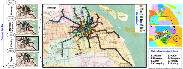
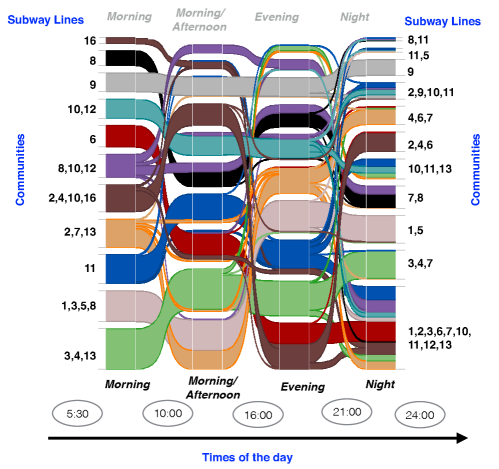
To characterise the properties of community snapshots, we start by analysing the daily community snapshots (which are the aggregate of the community snapshots of the four periods) for the studied month. Of the 18 working days, the daily community snapshots are the same for 17 days; the exception is the first working day after a holiday (Qing-ming Day). The common daily community snapshots for each period are shown in Fig. 1. Each period is represented by a snapshot; the changing colours of the station nodes show the communities joining and splitting over the four periods. To be more specific, Fig. 2 shows the community snapshots of the subway system that appear to represent 94% of working days. The subway lines that make up each community are displayed. The relationships between subway lines and administrative divisions are given in Tab. S1. The subway lines that pass through the city centre are likely to construct communities with other subway lines that are associated with residential, tourist and business areas. For example, in the morning, five of the six communities with more than two subway lines include subway lines 10 and 13, which cross the city centre, as described in Tab. S1. Furthermore, the number of stations in each community class is relatively stable, with one more or less between adjacent periods. However, the snapshots of the communities over all four periods (morning, morning/afternoon, evening and night) do not conform to this pattern, as stations in the last period join other communities. The mixing of communities is particularly obvious in the evening. For example, the black community (subway line 8) in the evening combines with the purple community (subway line 8, 10 and 12). Thus, no single community snapshot accurately shows the interactions between stations throughout a working day. The changes reveal passengers’ various activities, and the decisions they make regarding where and when to travel.

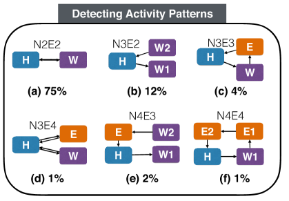
Thus we further study passengers’ activities. Due to the relatively small passenger volume in the night, as shown in Fig. S2, we mainly study evening behaviour; a snapshot of evening communities is shown in Fig. 1, which also has additional information on administrative divisions. Our analysis focuses on workers who start the first trip before 10:00 and make other trips after 17:00, as their activity patterns reflect regular behaviour. The high-order structure of their activity patterns is described in Fig. 3. We label each activity pattern by their number of nodes and edges. For example, the pattern N2E2 denotes an activity pattern with two Nodes and two Edges. We find that the activity pattern of N2E2 is the most common, followed by N3E2 (with three nodes and two edges) and others. Each activity pattern describes a daily activity scenario. For example, the pattern N3E2 describes an individual who goes from home H to workplace W1, then back home after work from place W2. The activity patterns in the subway system show that most (85%) individuals tend to go home after work, following pattern N2E2. Only a few people (around 15%) go to other places after work. We conclude that an activity with more edges has less probability of occurring. This is consistent with previous studies of other cities, such as Singapore [41], Paris [42] and Chicago [42].

Exploring the where and when dimensions

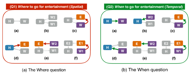
The community snapshot approach can improve our ability to measure the dynamics of mobility flows. However, the spatial-temporal models that drive the mobility dynamics are still unclear. From morning to afternoon, individuals’ spatial and temporal activities are stable, as they have fixed homes and workplaces. However, in the evening, travel to entertainment places is unstable. Thus we further analyse the evening activities by exploring the where and when dimensions, as shown by the coloured edges shown in Fig. 4 (a) and Fig. 4 (b), respectively . Next, we describe them separately.

Exploring the where dimension

First, we analyse the emotional strength of each station in the eight administrative divisions of Shanghai. Specifically, the distribution of emotion for each station is described in Fig. 5 (a) which shows a heterogeneous spatial distribution. The colours vary from blue to red. For each station, the redder the colour, the more positive the emotion. We find that the stations in the city centre around the ’Jing’an’ and ’Huangpu’ divisions have higher positive emotions than the outer divisions.

Then, we apply the microblog-based spatial model to different groups of administrative divisions, as shown in Tab. 1. The correlation weight is a value between 0 and 1. The larger the correlation, the more accurately the model describes the reality. We find that the divisions near the city centre have higher correlations than divisions on the edge of the city. Specifically, the model of the stations in the city centre has the highest correlation with reality. In contrast, the gravity mobility model [43] is much less accurate, with correlations around 0.1 in all three groups shown in Tab. 1. These results suggest that considering the heterogeneous spatial popularity of stations in addition to the influence of distance can improve the description of individuals’ spatial mobility flows.

Table 1: Correlations of the real mobility flows between stations with the predictions of the spatial model. There are two groups (’Centre’ and ’Outer’) of administrative divisions. ’Centre’ divisions are divisions 1 to 4 in Fig. 1, whereas ’Outer’ divisions are 5 to 8 in Fig. 1. A third group, which combines the two groups, is labelled ’Centre&Outer’.

	Pearson’s correlations	95% confidence interval of Pearson’s correlations
Centre&Outer	0.32	0.31 $\sim$ 0.32
Centre	0.35	0.34 $\sim$ 0.36
Outer	0.30	0.29 $\sim$ 0.31

Exploring the when dimension

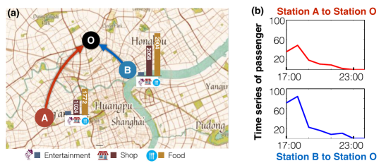
To investigate the temporal mobility flow, especially in the evening, we further explore the underlying temporal model by considering the influence of the environment. The model examines the influence of different types of places by varying the facilities, such as the food-related facilities shown in Fig. 5 (b). Fig. 6 presents two samples of mobility flows that each have two origins and one destination. The two origins are in different environments with different facilities around the stations, which may play a role in individuals’ temporal decision making.

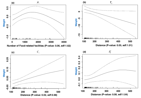
To identify the meaningful characteristics of facilities, we first use training samples (80% of all of the samples)to analyse the correlations between the spatial facilities and the parameters in the temporal model. The samples are shown in the x-axis of Fig. 7. A $p$ -value for a model’s smooth term that is less than or equal to 5% or 1% indicates that the chosen smooth term is significant. Moreover, the estimated degree of freedom (edf) for the smooth terms’ significance is estimated. When the value of the edf is far from 1, the smooth item tends to reflect a nonlinear relationship. In this study, keeping only the significant features ( $p$ -value $<$ 0.1), we find that only the food-related feature, with $P$ -value 0.06, has an obvious correlation with $\mu$ . The edf is far from 1, indicating a nonlinear relationship between individuals’ perceptions of travelling discomfort and the presence of food-related facilities, as shown in Fig. 7. Individuals near stations with a higher $\mu$ tend to have lower travelling discomfort when the number of food-related facilities is near 1563. As the number of food-related facilities increases, $\mu$ first increases, then decreases, indicating that a moderate number of food-related facilities has the greatest influence. As for the perception ( $\tau$ ) of delay cost, distance plays an obvious role, with a $p$ -value of $<$ 0.05. $\tau$ ’s edf of the smooth term on distance is near 1, indicating a linear relationship between perception of delay cost and distance. Specifically, as shown in Fig. 7, individuals near stations with higher $\tau$ values tend to start their travel earlier. The other two parameters ( $C$ and $P_{0}$ ) are only related to distance, with which they have a positive linear relationship.

In addition, applying the correlations learned by the training samples, we use the testing samples (20% of all samples) to examine whether it is possible to simulate the temporal flows with the inferred parameters. There are 17 pairs of stations in the testing sample. We mainly study their temporal flows in the evening after work (from 17:00 to 24:00). The simulation result is shown in Fig. S1. As we see, the simulation based on the temporal model driven by the desire to balance travelling comfort and delay cost is much closer to the real temporal flows. This result shows that our temporal model describes to some extent the real temporal mobility flows, and can take into account the influences of the environment on individuals’ perceptions.

Discussion

To study the dynamics of mobility flows in urban transport it is important to estimate the spatial and temporal interactions of human mobility flows between stations. Understanding these flows helps planners to evaluate traffic congestion [44], and avoid the dangers of overcrowding [45]). Taking the subway system of Shanghai as a case study, we used community snapshots to investigate the variability of spatial-temporal mobility flows on working days. The results show that the flows change at different times of day, but the patterns are similar on each working day. Recognising these dynamics will help to predict human movements between stations on spatial-temporal scales, which may help planners to efficiently schedule subway cars.

To further understand the models, we investigate the high-order structure of activity patterns in both the temporal and spatial dimensions. Specifically, we use the patterns in passengers’ travelling activities to determine passengers’ lifestyle needs and then investigate (1) the where (spatial) dimension of mobility flows between subway stations by correlating microblog topics with spatial popularity and (2) the when (temporal) dimension of individual schedules of activities by correlating spatial facilities and travelling distance with the perceptions of travelling discomfort and delay cost. We argue that correlations between the stations and their environments may to some extent be explained by urban catalyst theory (first proposed in 1960 [46] and fully developed in 2000 [47]). According to this theory, railway stations can act as urban catalysts and have positive effects on their surroundings, but are also influenced by their surroundings [48, 34, 49]. Therefore, a boom in living/business buildings or popular locations around a subway station can increase its traffic flows, as appears to be the case in Shanghai[34], Seoul[33], Kun Dae Yeok[50] and Toronto [51]. Note that the nonlinear relationship between $\mu_{i}$ and food-related facilities, shown in Fig. 7, indicate that although the overall influence of food-related facilities is related to the quantity of facilities, more is not necessarily better. Once the number of food-related facilities in a specified spatial area exceeds a threshold, which may vary with the size of the area, many small but low-level food-related facilities may appear, thus decreasing the total influence of food-related facilities. This study has some limitations. Community snapshots of the Shanghai subway system are used as a case study, and the dataset contains information for only one month. Other patterns may be found with data covering a longer time period. However, the same methods analysis of could be used. In this study, we focus on community snapshots of the subway system; future studies could consider the similarity and differences of the patterns in other public transit systems. Furthermore, in this study we only analyse the correlations of individual spatial-temporal perceptions with the environment. The causal relationships should be examined in future studies. In this study we characterise the environment by counting the number of various kinds of facilities, but do not consider their scales. Thus we do not sufficiently capture the correlation with entertainment and shopping facilities, as their effect on individuals’ perceptions cannot be measured by simply counting the facilities. Better measures are needed to further analyse their effect.

Methods

Data

To study our tasks, we use the travel smart card dataset from Shanghai, China for the month of April 2015. Items (such as card number, transaction date, transaction time, station name and transaction amount) are recorded by the subway system. The dataset contains information about 313 subway stations, 11 million individuals and around 120 million trips. We define the morning period as from 5:30 to 09:59, and the evening period from 16:00 to 20:59. Both periods are approximately 5 hours. The two time periods between these periods are labelled morning/afternoon and night. A trip is only counted as belonging to a given period if both the starting time and end time occur within the same period. More details can be found in the Supplement $\S 2.1$ .

Baidu APIs [38] is used to identify the 2 million spatial facilities within 1 km of a subway station. The spatial facilities are assigned to one of three categories (entertainment, shopping and food) according to their business type. We also use the Weibo APIs[39] to identify 1 million microblogs generated near the stations. To identify the topics of these microblogs, we use the Topic Expertise Model, an improved Latent Dirichlet allocation (LDA) topic model for the detection of keywords [52]; we use the groups of microblogs generated near each station as files. Finally, we determine the distribution of topics across the subway system using the word distribution in each topic. See Supplement $\S 2.1$ for details.

Mining community snapshots

To address the technical challenges of the community snapshot analysis for each period, we use community detection methods. The community snapshot analysis constitutes four steps. For each day, there are different temporal scales of flow matrices, representing the directed mobility flows between any two stations at a certain temporal scale. In this study, we focus on the temporal scale of four periods in a day. Through community detection and consensus analysis of each period, we can build a matrix of community identification for each station, producing a community matrix for each period. With the help of clustering methods, we can identify the categories of these community snapshots. See Supplement $\S 2.2$ for details.

Spatial and temporal models for the where and when dimensions

We adopt a dual-perspective on passengers’ activity patterns to investigate the spatial and temporal dimensions of individuals travelling decision making. Specifically, we examine where and when individuals go for entertainment in the evening, by introducing an individual-based model. Specifically, we use microblogs, which reflect individuals’ relevant perceptions of popularity and distance, to determine the heterogeneous spatial popularity $X_{j}^{i}$ of each topic at every station. This results in a spatial model based on the location-based mobility model.

To study the temporal model of individual schedules of activities, we use the difference equations of temporal flows to model the dynamic evolution of balancing travelling comfort and delay cost, which are correlated with environment and distance. Let $Y_{t}^{i}$ denote the travelling volume from the $i$ -th station at time $t$ . Thus $Y_{t}^{i}$ is modelled as $Y_{t}^{i}=N_{i}(\tau_{i}\Delta t-\mu_{i}Y_{t-1}^{i}+C_{i})$ . Here let $\mu_{i}$ refers to individuals’ perceptions of the travelling discomfort in the $i$ -th station, correlated with the nearby economic/social buildings. $\tau_{i}$ refer to individuals’ perceptions of the delay cost, correlated with the distances between stations. $N_{i}$ denotes the total volume of passengers in station $i$ in the evening. Thus individual’s temporal choice at time $t$ has a probability of $p_{t}^{i}=Y_{t}^{i}/N_{i}$ . In addition, these parameters (such as $\mu_{i}$ and $\tau_{i}$ ) are further correlated with features (such as economic/social buildings and distances) by the generalised additive model. See Supplement $\S 2.3$ for more details.

References

[1] Batty, M. et al. A theory of city size. Science 340, 1418–1419 (2013).
[2] Batty, M. The size, scale, and shape of cities. Science 319, 769–771 (2008).
[3] Rodrigue, J.-P., Comtois, C. & Slack, B. The Geography of Transport Systems (2nd Edition) (Routledge, 2009).
[4] Zhong, C., Manley, E., Arisona, S. M., Batty, M. & Schmitt, G. Measuring variability of mobility patterns from multiday smart-card data. J.Comput.Sci. 9, 125–130 (2015).
[5] Newman, M. E. The structure and function of complex networks. SIAM Rev. Soc. Ind. Appl. Math. 45, 167–256 (2003).
[6] Sun, L., Jin, J. G., Axhausen, K. W., Lee, D.-H. & Cebrian, M. Quantifying long-term evolution of intra-urban spatial interactions. J. R. Soc. Interface 12, 20141089 (2015).
[7] Zhong, C., Arisona, S. M., Huang, X., Batty, M. & Schmitt, G. Detecting the dynamics of urban structure through spatial network analysis. Int. J. Geogr. Inf. Sci. 28, 2178–2199 (2014).
[8] Kim, K., Oh, K., Lee, Y. K., Kim, S. & Jung, J.-Y. An analysis on movement patterns between zones using smart card data in subway networks. Int. J. Geogr. Inf. Sci. 28, 1781–1801 (2014).
[9] De Palma, A., Kilani, M. & Proost, S. Discomfort in mass transit and its implication for scheduling and pricing. Transport. Res. B-Meth. 71, 1–18 (2015).
[10] Paldino, S., Bojic, I., Sobolevsky, S., Ratti, C. & González, M. C. Urban magnetism through the lens of geo-tagged photography. EPJ Data Sci. 4, 1 (2015).
[11] Austwick, M. Z., O’Brien, O., Strano, E. & Viana, M. The structure of spatial networks and communities in bicycle sharing systems. PLoS ONE 8, e74685 (2013).
[12] Borgnat, P. et al. A dynamical network view of lyon’s vélo’v shared bicycle system. In Dynamics On and Of Complex Networks, vol.2,267–284 (Springer, 2013).
[13] Chatterjee, A. Studies on the structure and dynamics of urban bus networks in indian cities. arXiv preprint arXiv:1512.05909 (2015).
[14] Zhang, H., Zhao, P., Wang, Y., Yao, X. & Zhuge, C. Evaluation of bus networks in china: From topology and transfer perspectives. Discrete. Dyn. Nat. Soc. 501, 328320 (2015).
[15] Liu, X., Gong, L., Gong, Y. & Liu, Y. Revealing travel patterns and city structure with taxi trip data. J. Transp. Geogr. 43, 78–90 (2015).
[16] Kang, C., Sobolevsky, S., Liu, Y. & Ratti, C. Exploring human movements in singapore: a comparative analysis based on mobile phone and taxicab usages. In Proceedings of the 2nd ACM SIGKDD International Workshop on Urban Computing, 1 (ACM, 2013).
[17] Diao, M., Zhu, Y., Ferreira, J. & Ratti, C. Inferring individual daily activities from mobile phone traces: A boston example. Environ. Plann B Plann. Des. 0265813515600896 (2015).
[18] Gong, L., Liu, X., Wu, L. & Liu, Y. Inferring trip purposes and uncovering travel patterns from taxi trajectory data. Cartogr. Geogr. Inf. Sci. 1–12 (2015).
[19] Alexander, L., Jiang, S., Murga, M. & González, M. C. Origin–destination trips by purpose and time of day inferred from mobile phone data. Transport. Res. C-Emerg. Technol. 58, 240–250 (2015).
[20] Jiang, S., Ferreira Jr, J. & Gonzalez, M. C. Discovering urban spatial-temporal structure from human activity patterns. In Proceedings of the ACM SIGKDD International Workshop on Urban Computing, 95–102 (ACM, 2012).
[21] Liang, X., Zhao, J., Dong, L. & Xu, K. Unraveling the origin of exponential law in intra-urban human mobility. Sci. Rep. 3 (2013).
[22] Yan, X.-Y., Zhao, C., Fan, Y., Di, Z. & Wang, W.-X. Universal predictability of mobility patterns in cities. J. R. Soc. Interface 11, 20140834 (2014).
[23] Goh, S., Lee, K., Park, J. S. & Choi, M. Modification of the gravity model and application to the metropolitan seoul subway system. Phys. Rev. E 86, 026102 (2012).
[24] Mendiola, L., González, P. & Cebollada, À. The link between urban development and the modal split in commuting: the case of biscay. J. Transp. Geogr. 37, 1–9 (2014).
[25] Haddad, E. A., Hewings, G. J., Porsse, A. A., Van Leeuwen, E. S. & Vieira, R. S. The underground economy: Tracking the higher-order economic impacts of the são paulo subway system. Transport. Res. A-Policy and Pract. 73, 18–30 (2015).
[26] Perkins, T. A. et al. Theory and data for simulating fine-scale human movement in an urban environment. J. R. Soc. Interface. 11, 20140642 (2014).
[27] Preoţiuc-Pietro, D., Lampos, V. & Aletras, N. An analysis of the user occupational class through twitter content (The Association for Computational Linguistics, 2015).
[28] Preoţiuc-Pietro, D., Volkova, S., Lampos, V., Bachrach, Y. & Aletras, N. Studying user income through language, behaviour and affect in social media. PLoS One 10, e0138717 (2015).
[29] Yuan, Q., Cong, G., Ma, Z., Sun, A. & Thalmann, N. M. Who, where, when and what: discover spatio-temporal topics for twitter users. In Proceedings of the 19th ACM SIGKDD International Conference on Knowledge Discovery and Data Mining, 605–613 (ACM, 2013).
[30] Mohring, H. Optimization and scale economies in urban bus transportation. Am. Econ. Rev. 62, 591–604 (1972).
[31] Kraus, M. Discomfort externalities and marginal cost transit fares. J. Urban. Econ. 29, 249–259 (1991).
[32] de Lapparent, M. & Koning, M. Analyzing time sensitivity to discomfort in the paris subway: an interval data model approach. Transportation 1–21 (2015).
[33] Bae, C.-H. C., Jun, M.-J. & Park, H. The impact of seoul’s subway line 5 on residential property values. Transport Policy 10, 85–94 (2003).
[34] Wang, T. & Lu, J. Railway station complex and urban catalyst—example of shanghai south railway station. In Urban Plan. Forum, vol. 4, 76–83 (2006).
[35] Hastie, T. J. & Tibshirani, R. J. Generalized Additive Models, vol. 43 (CRC Press, 1990).
[36] Wood, S. Generalized Additive Models: An Introduction with R (CRC press, 2006).
[37] Seasson information technology Co. Ltd. Shanghai open data apps (2015). URL {http://soda.datashanghai.gov.cn/}. Online; accessed January 18, 2016.
[38] Inc., B. Javascript api (2016). URL {http://lbsyun.baidu.com/index.php?title=jspopular}. Online; accessed August 31, 2016.
[39] Weibo, S. Api document (2016). URL {http://open.weibo.com/wiki/}. Online; accessed August 31, 2016.
[40] wikipedia. Shanghai (2016). URL {https://en.wikipedia.org/wiki/Shanghai/}. Online; accessed August 31, 2016.
[41] Jiang, S., Ferreira Jr, J. & González, M. C. Activity-based human mobility patterns inferred from mobile phone data: A case study of singapore. In Proceedings of the 4th International Workshop on Urban Computing (2015).
[42] Schneider, C. M., Belik, V., Couronné, T., Smoreda, Z. & González, M. C. Unravelling daily human mobility motifs. J. R. Soc. Interface. 10, 20130246 (2013).
[43] Alonso, W. A theory of movements: Introduction (1976). Working Paper No. 266, Institute of Urban and Regional Development, University of California, Berkeley, CA.
[44] Ceapa, I., Smith, C. & Capra, L. Avoiding the crowds: understanding tube station congestion patterns from trip data. In Proceedings of the ACM SIGKDD International Workshop on Urban Computing, 134–141 (ACM, 2012).
[45] Pearl, T. H. Crowd crush: How the law leaves american crowds unprotected. SSRN (2015).
[46] Jacobs, J. The Death and Life of Great American Cities (Vintage, 1961).
[47] Davis, J. Urban catalysts in theory and practice. Archit. Res. Q. 13, 295–306 (2009).
[48] Geng, L. Effect of subway development on consumption space of big cities. City Plan. Rev. 3, 17–24 (2009).
[49] Papa, E., Pagliara, F. & Bertolini, L. Rail system development and urban transformations: Towards a spatial decision support system. In Railway Development: Impacts on Urban Dynamics, 337–357 (Physica-Verlag HD, 2008).
[50] Lee, H. Accessibility and land use changes around subway stations: case study of kun dae yeok. Korean J. Geogr. 32, 69–90 (1997).
[51] Dewees, D. N. The effect of a subway on residential property values in toronto. J. Urban. Econ. 3, 357–369 (1976).
[52] Yang, L. et al. Cqarank: jointly model topics and expertise in community question answering. In Proceedings of the 22nd ACM International Conference on Information & Knowledge Management, 99–108 (ACM, 2013).

Acknowledgements (not compulsory)

The authors are grateful to Dr Yongjian Yang for his valuable support of high performance computing cluster.

Author contributions statement

J.L. , B.Y. and Z.D. defined the problem. Z.D. J.L. and Y.B. discussed the method. Z.D. implemented and refined the method and conducted the experiments.All authors reviewed the manuscript.

Additional information

Competing financial interests: The authors declare no competing financial interests. Supplement can be found in URL: https://www.overleaf.com/read/qbdzxhsgfmbm