Monte Carlo determination of the low-energy constants for a two-dimensional spin-1 Heisenberg model with spatial anisotropy

Abstract

The low-energy constants, namely the spin stiffness $\rho_{s}$, the staggered magnetization density ${\cal M}_{s}$ per area, and the spinwave velocity $c$ of the two-dimensional (2D) spin-1 Heisenberg model on the square and rectangular lattices are determined using the first principles Monte Carlo method. In particular, the studied models have antiferromagnetic couplings $J_{1}$ and $J_{2}$ in the spatial 1- and 2-directions, respectively. For each considered $J_{2}/J_{1}$, the aspect ratio of the corresponding linear box sizes $L_{2}/L_{1}$ used in the simulations is adjusted so that the squares of the two spatial winding numbers take the same values. In addition, the relevant finite-volume and -temperature predictions from magnon chiral perturbation theory are employed in extracting the numerical values of these low-energy constants. Our results of $\rho_{s1}$ are in quantitative agreement with those obtained by the series expansion method over a broad range of $J_{2}/J_{1}$. This in turn provides convincing numerical evidence for the quantitative correctness of our approach. The ${\cal M}_{s}$ and $c$ presented here for the spatially anisotropic models are new and can be used as benchmarks for future related studies.

I Introduction

During the last three decades, the two-dimensional (2D) spin-1/2 Heisenberg model and its generalizations have been investigated in great detail both analytically and numerically Cana92 ; Oit941 ; Oit942 ; Wie94 ; San97 ; Bea96 ; Jia08 ; Jia11.2 . This is because these models are regarded as the relevant models for the 2D quantum antiferromagnets. Furthermore, although the phase diagram of high temperature cuprate superconductors is not well understood, it is generally believed that these cuprate superconductors may be obtained by doping the quantum antiferromagnetic insulators with charge carriers. As a result, research related to these models is still very active even today.

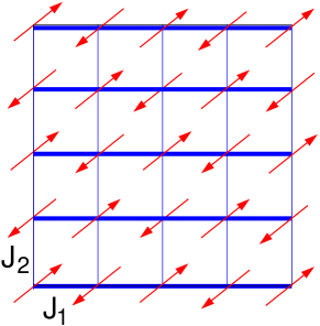
In addition to the spin-1/2 Heisenberg model, higher spin antiferromagnets, in particular the spin-1 Heisenberg model, are of theoretical interest due to the fact that they are relevant in explaining experimental results of real materials as well Ren87 ; Yam95 ; Mon96 ; Hon97 ; Hag98 ; Hon98 ; Uch99 ; Nar01 . For example, NDMAZ, NENP, and PbNi₂V₂O₈ are found to be spin-1 quasi-one-dimensional antiferromagnets. Besides the simplest type of these models which have spatially isotropic couplings, the spatially anisotropic Heisenberg models are also studied thoroughly Hal831 ; Hal832 ; Aff87 ; Sin88 ; Sak89 ; Egg94 ; Kat94 ; Yam951 ; Kit96 ; Koh98 ; Kog00 ; Kim00 ; Matsumoto02 ; Wan05 ; Wen09 ; Pardini08 ; Jia09 . In particular, these generalized models are frequently used as a route for studying quantum phase transitions. Moreover, the spatially anisotropic models are important in understanding experimental data. Two notable examples are the 2D spin-1/2 Heisenberg model with antiferromagnetic couplings $J_{1}$ and $J_{2}$ on the square and rectangular lattices as depicted in fig. 1, and the three-dimensional (3D) quantum antiferromagnet with a ladder pattern of spatial anisotropy on a cubic lattice. The former is argued to be relevant to the newly discovered pinning effects of the electronic liquid crystal in the underdoped cuprate superconductor YBa₂Cu₃O_6.45 Hinkov2007 ; Hinkov2008 , and the latter is considered to be the right model for explaining the phase diagram of TlCuCl₃ under pressure Rue03 ; Rue08 ; Jin12 ; Oit12 ; Kao13 ; Mer14 . To conclude, despite their simplicity, the spatially anisotropic Heisenberg models are among the most important and frequently studied systems in condensed matter physics.

Among the spatially anisotropic Heisenberg models with quantum spin, the one shown in fig. 1 is particularly special. For this model one sees clearly that as the magnitude of the ratio of couplings $J_{2}/J_{1}$ decreases, the system will eventually become decoupled one-dimensional (1D) antiferromagnetic chains (This takes place when $J_{2}/J_{1}=0$). One intriguing physics to explore for this spin-1/2 model is to examine whether a phase transition, between the antiferromagnetic and dimerized phases, occurs before one reaches the extreme case $J_{2}/J_{1}=0$. Analytic (and some numerical) evidence indicates that for the model of fig. 1 with quantum spin, the long-range antiferromagnetic order is destroyed only for infinitesimal $J_{2}/J_{1}$ Aff94 ; Aff96 . As a result, to study whether a phase transition appears at a particular value of $J_{2}/J_{1}>0$ using unbiased quantum Monte Carlo simulations is subtle. Indeed, as suggested in Refs. Matsumoto02 ; San99 , square lattice is not the appropriate lattice geometry for studying this model and rectangular lattice should be used instead. Furthermore, to capture the 2D characters of the model, the ratio of linear lattice sizes $L_{2}/L_{1}$ needs to be adjusted individually for each considered $J_{2}/J_{1}$. Even so, one must carry out careful investigation for the relevant observables so that the correct physics is obtained. For example, to make sure that the extrapolating results are reliable, for every $J_{2}/J_{1}$ several ratios of $L_{2}/L_{1}$ may be needed in the calculations.

For the spin-1/2 model depicted in fig. 1, one proposed quantitative approach to study the 2D ground state properties for every considered $J_{2}/J_{1}$ is to adjust the corresponding ratio $L_{2}/L_{1}$ so that the spatial winding number squared in the 1- and 2-directions, namely $\langle W_{1}^{2}\rangle$ and $\langle W_{2}^{2}\rangle$ take the same values. With such a method the 2D characters of the model will not be lost and can be obtained unbiasedly. This idea and similar ones have been used to study the spin-1/2 model (of fig. 1) Jia09 as well as quantum phase transitions of 2D dimerized quantum spin models Jia12 ; Shi13 .

The motivation of our study presented here is to provide a more convincing numerical result to support the quantitative correctness of the method of requiring $\langle W_{1}^{2}\rangle=\langle W_{2}^{2}\rangle$ in the simulations. Indeed, for the model in fig. 1 with quantum spin, Monte Carlo and series expansion results of the observable spin stiffness in the 1-direction agree with each other only for $J_{2}/J_{1}>0.4$ Jia09 . Therefore it is desirable to carry out a more detailed investigation so that the validity of this method can be justified. Notice it is known that the quantum phase transition associated with dimerization for the spin-1 model with the same spatial anisotropy takes place at a finite value of $J_{2}/J_{1}$ Matsumoto02 . Hence simulating the spin-1 model with the same spatial anisotropy shown in fig. 1 provides a great opportunity to further examine the validity of this method. Indeed as we will demonstrate later, our Monte Carlo results of $\rho_{s1}$ for the spin-1 model agree quantitatively with those determined by the series expansion method from $J_{2}/J_{1}=1$ down to $J_{2}/J_{1}\sim 0.08$ Pardini08 . Consequently our investigation gives convincing evidence for the correctness of this method.

Notice the spatially anisotropic quantum Heisenberg model of fig. 1 and its 1D limit are two completely different systems Cha89 ; Neu89 ; Has90 ; Has91 ; Egg94 ; Has93 . Therefore an unconventional behavior is likely to appear as one approaches the 1D limit from the 2D model. Our study paves a way to investigate the novel phenomena of dimension crossover from a 2D system to its 1D limit. We would like to point out that even with the method of adjusting the aspect ratio $L_{2}/L_{1}$ in the calculations so that the two spatial winding numbers squared reach the same numbers, the determination of ground state bulk properties requires the simulations being conducted at very low temperatures. Such zero temperature calculations are computationally demanding. Therefore instead of performing the simulations at very low temperatures and using the conventional approach of fitting the data with polynomials of the relevant parameters, we carry out the calculations at finite temperatures and employ the relevant predictions from magnon chiral perturbation theory (m$\chi$PT) to extract the bulk properties of the considered model. Later we will briefly argue that under certain circumstances, this approach seems to be more efficient than the conventional one. Indeed, for each considered $J_{2}/J_{1}$, a few tens of the corresponding data points can be described quantitatively by two equations with only three unknown parameters, and particularly, we are able to arrive at high precision results with moderate computing resources. Finally, another remarkable finding in our investigation is that, the m$\chi$PT can also be used to examine unambiguously the presence of the long-range antiferromagnetic order. This will be explained in more detail in the relevant section.

Figure 1: The two-dimensional (2D) spatially anisotropic spin-1 Heisenberg model on the square and rectangular lattices investigated in this study.

This paper is organized as follows. First, after the introduction, the spatially anisotropic spin-1 Heisenberg model and the observables considered in this work are detailed. Furthermore, the m$\chi$PT is briefly introduced and some of its predictions relevant to our study are also listed. We then present the data as well as the resulting numerical results based on these data. Finally a section is devoted to conclude our investigation.

II Microscopic Models and Corresponding Observables

The 2D spin-1 Heisenberg model we consider in this study is defined by the Hamilton operator

$$H=\sum_{x}\Big{[}\,J_{1}\vec{S}_{x}\cdot\vec{S}_{x+\hat{1}a}+J_{2}\vec{S}_{x}\cdot\vec{S}_{x+\hat{2}a}\,\Big{]},$$ (1)

and is depicted by fig. 1. In Eq. (1), $\hat{1}$ and $\hat{2}$ refer to the two spatial unit-vectors and $a$ is the lattice spacing. In addition, $J_{1}$ and $J_{2}$ are the antiferromagnetic couplings in the $1$- and $2$-direction, respectively. Finally the $\vec{S_{i}}$ shown above is a spin-1 operator at site $i$.

A physical quantity measured in our simulations is the staggered susceptibility $\chi_{s}$, which is given by

$$\chi_{s} = \frac{1}{L_{1}L_{2}}\int_{0}^{\beta}dt\ \frac{1}{Z}\mbox{Tr}[M^{3}_{s}(0)M^{3}_{s}(t)\exp(-\beta H)].$$ (2)

Here $\beta$ is the inverse temperature, $L_{1}$ and $L_{2}$ are the spatial box sizes in the $1$- and $2$-direction, respectively, and $Z=\mbox{Tr}\exp(-\beta H)$ is the partition function. Furthermore, $M^{3}_{s}$ appearing in Eq. (2) is the third component of the staggered magnetization $\vec{M}_{s}=\sum_{x}(-1)^{x_{1}+x_{2}}\vec{S}_{x}$. Another observables considered here is the uniform susceptibility $\chi_{u}$, which takes the form

$$\chi_{u} = \frac{1}{L_{1}L_{2}}\int_{0}^{\beta}dt\ \frac{1}{Z}\mbox{Tr}[M^{3}(0)M^{3}(t)\exp(-\beta H)].$$ (3)

Here $\vec{M}=\sum_{x}\vec{S}_{x}$ is the uniform magnetization. Both $\chi_{s}$ and $\chi_{u}$ can be measured very efficiently with the loop-cluster algorithm using improved estimators Wie94 .

Notice both of these two observables can be expressed in quantities related to the clusters. In particular, $\chi_{u}$ is associated with the temporal winding number $W_{t}=\sum_{\cal C}W_{t}({\cal C})$ which is the sum of winding numbers $W_{t}({\cal C})$ of the loop-clusters ${\cal C}$ around the Euclidean time direction. Similarly, the spatial winding numbers $W_{i}$ for $i\in\{1,2\}$ are defined in the same manner. With the convention employed here, the spin stiffness $\rho_{s}$ (for $J_{2}/J_{1}=1$) can be obtained directly from the standard relation $\rho_{s}=\frac{3}{4\beta}\left(\langle W_{1}^{2}\rangle+\langle W_{2}^{2}\rangle\right)$ in the zero-temperature and infinite-volume limits. In addition, the temporal winding number squared $\langle W_{t}^{2}\rangle$ calculated in this study is exactly the susceptibility $\chi$ and is related to $\chi_{u}$ by $\chi_{u}=\frac{\beta}{L_{1}L_{2}}\langle W_{t}^{2}\rangle$. Finally the spinwave velocity $c$ can be estimated from these winding numbers squared by the method detailed in Refs. Jia11.1 ; Sen15 ; Kao13 .

III Low-Energy Effective Theory for Magnons

In this section we summarize the relevant theoretical predictions, namely the finite-volume and -temperature expressions of $\chi_{s}$ and $\chi_{u}$ from m$\chi$PT Cha89 ; Neu89 ; Has90 ; Has91 ; Has93 . These predictions are used to calculate the desired low-energy constants. Due to the spontaneous breaking of the $SU(2)_{s}$ spin symmetry down to its $U(1)_{s}$ subgroup, the low-energy physics of antiferromagnets is governed by two massless Goldstone bosons, the magnons. The systematic low-energy effective field theory for magnons is formulated in term of the staggered magnetization. The staggered magnetization of an antiferromagnet is described by a unit-vector field $\vec{e}(x)$ in the coset space $SU(2)_{s}/U(1)_{s}=S^{2}$, i.e. $\vec{e}(x)=\big{(}e_{1}(x),e_{2}(x),e_{3}(x)\big{)}$ with $\vec{e}(x)^{2}=1$. Here $x=(x_{1},x_{2},t)$ denotes a point in (2+1)-dimensional space-time. To leading order, the Euclidean magnon low-energy effective action takes the form

$$S[\vec{e}\,] = \int^{L_{1}}_{0}dx_{1}\int^{L_{2}}_{0}dx_{2}\int^{\beta}_{0}\ dt\ \left(\frac{\rho_{s1}}{2}\partial_{1}\vec{e}\cdot\partial_{1}\vec{e}\right.$$ (4)

$$+\left.\frac{\rho_{s2}}{2}\partial_{2}\vec{e}\cdot\partial_{2}\vec{e}+\frac{\rho_{s}}{2c^{2}}\partial_{t}\vec{e}\cdot\partial_{t}\vec{e}\right),$$

where the index $i\in\{1,2\}$ labels the two spatial directions and $t$ refers to the Euclidean time-direction. The temporal spin stiffness $\rho_{s}$ is given by $\rho_{s}=\sqrt{\rho_{s1}\rho_{s2}}$, where $\rho_{s1}$ and $\rho_{s2}$ are the spin stiffness in the spatial directions. Finally, the parameter $c$ in Eq. (4) is the spinwave velocity. Notice the physical quantities, namely $\rho_{s}$, $\rho_{s1}$, $\rho_{s2}$, and c appearing inside Eq. (4) are the bulk ones Has93 . By introducing $x^{\prime}_{1}=(\rho_{s2}/\rho_{s1})^{1/4}x_{1}$ and $x^{\prime}_{2}=(\rho_{s1}/\rho_{s2})^{1/4}x_{2}$, Eq. (4) can be rewritten as

$$S[\vec{e}\,] = \int^{L^{\prime}_{1}}_{0}dx^{\prime}_{1}\int^{L^{\prime}_{2}}_{0}dx^{\prime}_{2}\int^{\beta}_{0}dt\ \frac{\rho_{s}}{2}\Big{(}\partial^{\prime}_{i}\vec{e}\cdot\partial^{\prime}_{i}\vec{e}$$ (5)

$$+\frac{1}{c^{2}}\partial_{t}\vec{e}\cdot\partial_{t}\vec{e}\Big{)}.$$

If one additionally requires $L^{\prime}_{1}=L^{\prime}_{2}=L$, then the condition of square area is obtained.

With the Euclidean action Eq. (5), the finite-volume and -temperature expressions of $\chi_{s}$ and $\chi_{u}$ in the cubical regime, where the condition $\beta c\approx L$ is met, are calculated in Ref. Has93 and take the following forms

$$\chi_{s} = \frac{{\cal M}_{s}^{2}L^{2}\beta}{3}\left\{1+2\frac{c}{\rho_{s}Ll}\beta_{1}(l)\right.$$ (6)

$$+\left.\left(\frac{c}{\rho_{s}Ll}\right)^{2}\left[\beta_{1}(l)^{2}+3\beta_{2}(l)\right]+O\left(\frac{1}{L^{3}}\right)\right\}$$

and

$$\chi_{u} = \frac{2\rho_{s}}{3c^{2}}\left\{1+\frac{1}{3}\frac{c}{\rho_{s}Ll}\widetilde{\beta}_{1}(l)+\frac{1}{3}\left(\frac{c}{\rho_{s}Ll}\right)^{2}\times\right.$$ (7)

$$\left.\left[\widetilde{\beta}_{2}(l)-\frac{1}{3}\widetilde{\beta}_{1}(l)^{2}-6\psi(l)\right]+O\left(\frac{1}{L^{3}}\right)\right\},$$

respectively. In Eqs. (6) and (7), the functions $\beta_{i}(l)$, $\widetilde{\beta}_{i}(l)$, and $\psi(l)$, which only depend on $l=(\beta c/L)^{1/3}$, are shape coefficients of the space-time box. The explicit formulas of these shape coefficients can be found in Ref. Has93 .

IV Determination of the Low-Energy Constants

In order to determine the low-energy constants as functions of $J_{2}/J_{1}$ for the 2D spatially anisotropic spin-1 Heisenberg model given by Eq. (1) (and depicted in fig. 1), we have performed simulations for $0.0435\leq J_{2}/J_{1}\leq 1.0$ with various box sizes using the loop algorithm Troyer08 ; Bau11 . The value of $J_{2}/J_{1}=0.0435$ is included in our consideration since it is slightly below the critical point $(J_{2}/J_{1})_{c}=0.043648(8)$ determined in Ref. Matsumoto02 . The results at $J_{2}/J_{1}=0.0435$ provide an opportunity to examine whether our Monte Carlo data at $J_{2}/J_{1}=0.0435$ can be captured quantitatively by the relevant predictions of m$\chi$PT. Without loss of generality, we have set $J_{1}=1.0$ in our Monte Carlo simulations. The cubical regime is determined by the condition $\langle W_{1}^{2}\rangle\approx\langle W_{2}^{2}\rangle\approx\langle W_{t}^{2}\rangle$. Notice Eqs. (6) and (7) are obtained for a (2+1)-dimensional box with equal extent in the two spatial directions. Since $J_{2}\leq J_{1}$ in our calculations, the box sizes $L_{1}$ and $L_{2}$ used in the simulations must satisfy $L_{2}\leq L_{1}$ so that the condition $\langle W_{1}^{2}\rangle\approx\langle W_{2}^{2}\rangle$ can be fulfilled. Finally interpolation of the data points is necessary as well in order to use Eqs. (6) and (7). After employing all these requirements in our calculations, the low-energy constants can be extracted by fitting the Monte Carlo data to the effective field theory predictions. First of all, in the next subsection we focus on our Monte Carlo results of the isotropic situation $J_{2}/J_{1}=1$.

IV.1 The low-energy constants for the isotropic model

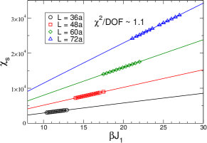
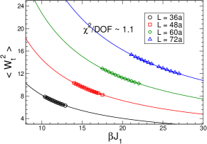
As a first step toward a high accuracy determination of the desired low-energy constants, the spinwave velocity $c$ is calculated through the square of winding numbers as suggested in Refs. Jia11.1 ; Sen15 . Specifically, for a given square lattice with linear box size $L_{1}$, one tunes the inverse temperature $\beta$ to a value $\beta^{\star}$ so that $\langle W_{1}^{2}\rangle\approx\langle W_{2}^{2}\rangle\approx\langle W_{t}^{2}\rangle$. Then the $c$ corresponding to this finite lattice is estimated to be $c\sim L_{1}/\beta^{\star}$. The numerical values of $c$ obtained by this method for several box sizes $L_{1}$ are given in table 1, and a weighted average of these values of $c$ leads to $c=3.0648(8)J_{1}a$. The result of $c$, namely $c=3.0648(8)J_{1}a$ reached here has (much) better precision than its early known Monte Carlo results Bea99 , and is in nice agreement with the spinwave theory estimate $c=3.067J_{1}a$ Oit942 . Furthermore, since for the isotropic case one can reach the condition $\langle W_{1}^{2}\rangle$ = $\langle W_{2}^{2}\rangle$ without performing any interpolation, we employ Eqs. (6) and (7) directly with a fixed $c=3.0648(8)J_{1}a$ to simultaneously fit the uninterpolated data of $\chi_{s}$ and $\langle W_{t}^{2}\rangle$. The numerical values of ${\cal M}_{s}$ and $\rho_{s}$ obtained from the fit are given by ${\cal M}_{s}=0.80460(4)/a^{2}$ and $\rho_{s}=0.8731(6)J_{1}$, respectively. In addition, the $\chi^{2}/{\text{DOF}}$ of this fit is around 1.0. Notice the ${\cal M}_{s}$ and $\rho_{s}$ calculated here also match excellently with ${\cal M}_{s}=0.80426/a^{2}$ and $2\pi\rho_{s}=5.461J_{1}$ determined by the spinwave theory. The results of the fit are shown in Fig. 2.

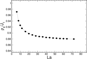
Besides the method of employing the predictions of m$\chi$PT, $\rho_{s}$ can be determined directly from the spatial winding numbers squared. Such a calculation of $\rho_{s}$ through $\langle W_{1}^{2}\rangle$ and $\langle W_{2}^{2}\rangle$ provides a good opportunity to verify the quantitative correctness of m$\chi$PT. Hence we have carried out new simulations with $J_{2}/J_{1}=1.0$ for several box sizes $L$ at low temperatures. The newly obtained $\rho_{s}$ data as a function of the box sizes $L$ is shown in Fig. 3. Remarkably, the $\rho_{s}$ determined from the spatial winding numbers squared is in quantitative agreement with that calculated using the predictions of m$\chi$PT. For instance, by applying polynomials up to third (fourth) order in $1/L$ to the relevant data of $6\leq L\leq 72$ ($6\leq L\leq 72$), we arrive at $\rho_{s}=0.8728(5)J_{1}$ ($\rho_{s}=0.8730(10)J_{1}$). These values of $\rho_{s}$ match nicely with those we calculated earlier using the related formulas from m$\chi$PT. To extract $\rho_{s}$ directly from the squares of spatial winding numbers, one has to obtain the zero-temperature values of the relevant observables. This is computationally demanding. In addition, it is also crucial to include as many data points as possible in the fits so that one can reach a accurate result of $\rho_{s}$. Hence when obtaining the ground state properties of a system is challenging, our approach, i.e. fitting the data using the relevant equations from m$\chi$PT, seems to be a more efficient way of calculating these low-energy constants since the related simulations are performed at finite-temperature and cubical regime.

$L_{1}/a$	$c/(J_{1}a)$
36	3.0645(11)
48	3.0647(16)
60	3.0651(16)
72	3.0647(15)

Table 1: The numerical values of $c$ at finite lattices for $J_{2}/J_{1}=1$. These results are obtained from the squares of spatial and temporal winding numbers.

Figure 2: Results of fitting the cubical regime data points of $\chi_{s}$ (top panel) and $\langle W_{t}^{2}\rangle$ (bottom panel) calculated at $J_{2}/J_{1}$ = $1$ to their m$\chi$PT predictions. The solid lines are obtained using the results from the fits.

Figure 3: The values of $\rho_{s}$ as a function of the box sizes $L$ for $J_{2}/J_{1}=1.0$. The results are obtained directly from the squares of spatial winding numbers and the dotted line is added to guide the eyes.

Figure 4: Results of fitting the cubical regime interpolated data points of $\chi_{s}$ calculated at $J_{2}/J_{1}$ = $0.8$, $0.6$, $0.4$, $0.2$, $0.1$, $0.08$, $0.06$, and $0.05$ to their m$\chi$PT predictions. The filled squares in the bottom panel are the uninterpolated data points determined at $J_{2}/J_{1}=0.0435$. The solid lines are obtained using the results from the fits. No result of m$\chi$PT fit associated with $J_{2}/J_{1}=0.0435$ is shown since such a fit is of poor quality.

Figure 5: Results of fitting the cubical regime interpolated data points of $\langle W_{t}^{2}\rangle$ calculated at $J_{2}/J_{1}$ = $0.8$, $0.6$, $0.4$, $0.2$, $0.1$, $0.08$, $0.06$, and $0.05$ to their m$\chi$PT predictions. The filled squares in the bottom panel are the uninterpolated data points determined at $J_{2}/J_{1}=0.0435$. The solid lines are obtained using the results from the fits. No result of m$\chi$PT fit associated with $J_{2}/J_{1}=0.0435$ is shown since such a fit is of poor quality.

Figure 6: The Monte Carlo results of ${\cal M}_{s}a^{2}$ (top panel) and $c/(J_{1}a)$ (bottom panel) as functions of $J_{2}/J_{1}$. The solid lines are added to guide the eyes.

IV.2 The low-energy constants for the anisotropic models

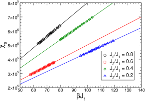
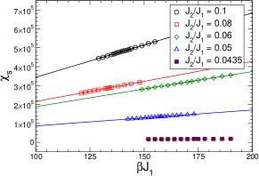
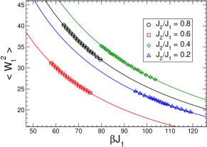
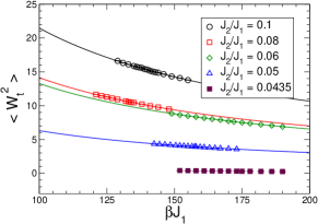
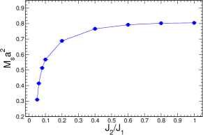
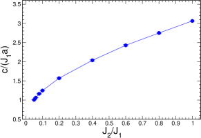
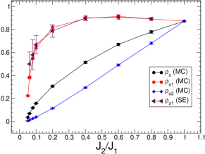
After having determined high precision values of ${\cal M}_{s}$, $\rho_{s}$, and $c$ for $J_{2}/J_{1}=1.0$, we turn to the calculations of these low-energy constants for the anisotropic models. Similar to the strategy used for the calculations associated with $J_{2}/J_{1}=1.0$, the numerical values of $c$ for various anisotropies $J_{2}/J_{1}$ considered here are determined using the square of winding numbers first. In particular, for each $J_{2}/J_{1}\neq 1.0$ the box sizes $L_{1}$ and $L_{2}$ as well as $\beta$ are chosen so that the condition $\langle W_{1}^{2}\rangle$ $\approx$ $\langle W_{2}^{2}\rangle$ $\approx$ $\langle W_{t}^{2}\rangle$ is satisfied. Notice interpolated data of $\chi_{s}$ and $\langle W_{t}^{2}\rangle$, based on the spatial winding numbers squared, are used in order to employ Eqs. (6) and (7) for the fits. In addition, the effective box sizes $L$ shown in Eqs. (6) and (7) are given by $L=\sqrt{L_{1}L_{2}}$. Figs. 4 and 5 demonstrate the results of the fits for all the considered $J_{2}/J_{1}$. The obtained ${\cal M}_{s}$, $\rho_{s}$, and $c$ are shown in table 2, figs. 6 and 7. Notice fig. 6 indicates that the antiferromagnetism is indeed weakened as one increases the anisotropy. Furthermore, the numerical values of $\rho_{s1}$ obtained from our Monte Carlo data and the series expansion results determined in Pardini08 are in nice agreement from $J_{2}/J_{1}=1$ down to $J_{2}/J_{1}\approx 0.08$. Although the truncation errors of series expansion results are large for small values of $J_{2}/J_{1}$, the outcomes of series expansion without the truncation errors agree very well with those of Monte Carlo for $J_{2}/J_{1}\geq 0.08$.

Interestingly, while for $J_{2}/J_{1}\geq 0.05$ the $\chi^{2}/{\text{DOF}}$ of the fits are smaller than 1.2, the fit using the data of $J_{2}/J_{1}=0.0435$ has a very poor quality. Specifically, we arrive at a $\chi^{2}/{\text{DOF}}\geq 38$ by fitting the interpolated data of $\chi_{s}$ and $\langle W_{t}^{2}\rangle$ calculated at $J_{2}/J_{1}=0.0435$ to Eqs. (6) and (7). This implies that the data of $\chi_{s}$ and $\langle W_{t}^{2}\rangle$ determined at $J_{2}/J_{1}=0.0435$ cannot be described by Eqs. (6) and (7), hence no antiferromagnetic order is present in the system. In other words, $J_{2}/J_{1}=0.0435$ is already beyond the critical point. This finding agrees with the conclusion obtained in Ref. Matsumoto02 that the critical point $(J_{2}/J_{1})_{c}$ is given by $(J_{2}/J_{1})_{c}=0.043648(8)$. Although $J_{2}/J_{1}=0.0435$ is only slightly away from $(J_{2}/J_{1})_{c}=0.043648(8)$, it is remarkable that the signal for the breaking down of the long-range antiferromagnetic order is persuasive. Interestingly, at $J_{2}/J_{1}=0.0435$ the magnitude of $\chi_{s}$ ($\langle W_{t}^{2}\rangle$) increases (decreases) with $\beta$ (The changes are not significant). This is similar to their expected behavior in the Néel phase. Hence, without the information of $(J_{2}/J_{1})_{c}=0.043648(8)$ and the result of poor fitting quality, one might naively conclude that $J_{2}/J_{1}=0.0435$ is still in the broken phase. We would like to emphasize the fact that with a careful analysis using the conventional approach, one still reaches the same conclusion that the long-range antiferromagnetic order is not present at $J_{2}/J_{1}=0.0435$.

To employ Eqs. (6) and (7) in our analysis, certain constraints such as large enough lattices must be fulfilled. Hence one may suspect that the poor fitting quality associated with the data at $J_{2}/J_{1}=0.0435$ is because the required conditions for the validity of Eqs. (6) and (7) are not met. To rule out this possibility, we have performed simulations on smaller lattices for $J_{2}/J_{1}=0.0435$. The $\chi^{2}/{\text{DOF}}$ for the newly determined data on smaller lattices is given by $\chi^{2}/{\text{DOF}}\geq 3.0$. Notice if the poor fitting quality associated with the data of $J_{2}/J_{1}=0.0435$ is rooted in the fact that the conditions for our simulations do not meet the validity requirement of Eqs. (6) and (7), then the fitting results related to the data of smaller lattices should have a worse $\chi^{2}/{\text{DOF}}$ than that of larger lattices. Hence, one should consider the poor fitting quality from the fit using the data obtained at $J_{2}/J_{2}=0.0435$ as a signal for the breaking down of antiferromagnetism. In summary, the results demonstrated in table 2, figs. 6 and 7 not only confirm the quantitative correctness of calculating the low-energy constants with the method employed here, these conclusions also provide convincing evidence that the m$\chi$PT can be applied efficiently to detect the breaking down of the long-range antiferromagnetic order.

$J_{2}/J_{1}$	$L_{1}$	$L_{2}$	${\cal M}_{s}a^{2}$	$\rho_{s}/J_{1}$	$c/(J_{1}a)$
1.0	100	100	0.80460(4)	0.8731(5)	3.0648(7)
0.8	206	180	0.8024(2)	0.779(12)	2.75(2)
0.6	180	132	0.7923(2)	0.670(11)	2.428(20)
0.4	244	140	0.7664(2)	0.514(9)	2.037(18)
0.2	272	102	0.6882(2)	0.3062(54)	1.570(13)
0.1	356	88	0.5680(2)	0.1582(23)	1.247(10)
0.08	332	72	0.5135(2)	0.119(2)	1.163(10)
0.06	416	76	0.4142(2)	0.0695(6)	1.0623(40)
0.05	390	64	0.3092(2)	0.03672(26)	1.0063(32)

Table 2: The numerical values of ${\cal M}_{s}$, $\rho_{s}$, and $c$ determined from the fits. $\rho_{s1}$ ($\rho_{s2}$) can be obtained by the relation $\rho_{s1}=\frac{L_{1}}{L_{2}}\rho_{s}$ ($\rho_{s2}=\frac{L_{2}}{L_{1}}\rho_{s}$). The $\chi^{2}/{\text{DOF}}$ for all the considered values of $J_{2}/J_{1}$ are smaller than 1.2 except for $J_{2}/J_{1}=0.0435$ which has a $\chi^{2}/{\text{DOF}}\geq 38$.

Figure 7: The Monte Carlo as well as the series expansion results of $\rho_{s1}$, $\rho_{s2}$, and $\rho_{s}$ as functions of $J_{2}/J_{1}$. The series expansion results shown in the figure are estimated from Ref. Pardini08 . The solid lines are added to guide the eyes.

V Conclusions and Discussions

In this study, we have calculated the low-energy constants, namely the spin stiffness $\rho_{s}$, the staggered magnetization density ${\cal M}_{s}$ per area, and the spinwave velocity $c$ of the spin-1 Heisenberg model with antiferromagnetic couplings $J_{1}$ and $J_{2}$ on the rectangular lattices using the quantum Monte Carlo simulations. The relevant finite-volume and -temperature predictions of m$\chi$PT are employed in extracting the numerical values of these low-energy constants. Such an approach is of computational efficiency as well, since the related simulations are conducted at finite temperatures. The precision of ${\cal M}_{s}$, $\rho_{s}$, and $c$ obtained here for $J_{2}/J_{1}=1.0$ is improved. Furthermore, the anisotropy $J_{2}/J_{1}$ dependence of ${\cal M}_{s}$, $\rho_{s}$ ($\rho_{s1}$), and $c$ are investigated in detail as well. In particular, the results of ${\cal M}_{s}$ and $c$ determined here for the spatially anisotropic models are new and can serve as benchmarks for future related studies. Our Monte Carlo and the series expansion results of $\rho_{s1}$ are in nice agreement for $J_{2}/J_{1}\geq 0.08$ Pardini08 . Consequently the quantitative correctness of our approach is justified. It is remarkable that the series expansion method leads to consistent values of $\rho_{s1}$ with those from Monte Carlo simulations in such strong anisotropic regime $J_{2}/J_{1}\geq 0.08$. We also confirm that the m$\chi$PT can be used efficiently to study the breaking down of long-range (antiferromagnetic) order. Specifically, for a considered relevant parameter, one can conclude that a phase transition from the long-range antiferromagnetic phase to a disordered phase already takes place before reaching that given parameter, if the fits using predictions of m$\chi$PT lead to poor fitting quality. Indeed, the outcomes of the fit using the data of $J_{2}/J_{1}=0.0435$ is consistent with the conclusion obtained in Ref. Matsumoto02 that the critical point $(J_{2}/J_{1})_{c}$ is given by $(J_{2}/J_{1})_{c}=0.043648(8)$. Considering the subtlety of quantitatively capturing the 2D characters of the spin-1/2 quantum Heisenberg model with the same spatial anisotropy as the one considered here, our study paves a way to unbiasedly investigate the novel phenomena of 2D to 1D dimension crossover of the related spin-1/2 model.

VI Acknowledgments

Simulations were done based on the loop algorithms in ALPS Troyer08 ; Bau11 . F.-J. J. is supported partially by MOST of Taiwan.

References

- (1) C. M. Canali, S. M. Girvin, and M. Wallin, Phys. Rev. B 45, 10131 (1992).
- (2) J. Oitmaa, C. J. Hamer, and Zheng Weihong, Phys. Rev. B 50, 3877 (1994).
- (3) C. J. Hamer, Zheng Weihong, and J. Oitmaa, Phys. Rev. B 50, 6877 (1994).
- (4) U.-J. Wiese and H.-P. Ying, Z. Phys. B 93, 147 (1994).
- (5) A. W. Sandvik, Phys. Rev. B 56, 18 (1997).
- (6) B. B. Beard and U.-J. Wiese, Phys. Rev. Lett. 77 (1996) 5130.
- (7) F.-J. Jiang, F. Kampfer, M. Nyfeler, and U.-J. Wiese, Phys. Rev. B 78, 214406 (2008).
- (8) F.-J. Jiang and U.-J.Wiese, Phys. Rev. B 83, 155120 (2011).
- (9) J. P. Renard, M. Verdaguer, L. P. Regnault, W. A. C. Erkelens, J. Rossat- Mignod, and W. G. Stirling, Europhys. Lett. 3, 945 (1987).
- (10) M. Yamashita, K. Inoue, T. Ohishi, T. Takeuchi, T. Yosida, and W. Mori, Mol. Cryst. Liq. Cryst. 274, 25 (1995)
- (11) M. Monfort, J. Ribas, X. Solans, and M. F. Bardia, Inorg. Chem. 35, 7633 (1996)
- (12) Z. Honda, K. Katsumata, H. Aruga Katori, K. Yamada, T. Ohishi, T. Manabe, and M. Yamashita, J. Phys.: Condens. Matter 9, 3487 (1997).
- (13) M. Hagiwara, Y. Narumi, K. Kindo, M. Kohno, H. Nakano, R. Sato, and M. Takahashi, Phys. Rev. Lett. 80, 1312 (1998).
- (14) Z. Honda, H. Asakawa, and K. Katsumata, Phys. Rev. Lett. 81, 2566 (1998).
- (15) Y. Uchiyama, Y. Sasago, I. Tsukada, K. Uchinokura, A. Zheludev, T. Hayashi, N. Miura, and P. Böni, Phys. Rev. Lett. 83, 632 (1999).
- (16) Y. Narumi, M. Hagiwara, M. Kohno, and K. Kindo, Phys. Rev. Lett. 86, 324 (2001).
- (17) F. D. M. Haldane, Phys. Lett. A93, 464 (1983).
- (18) F. D. M. Haldane, Phys. Rev. Lett. 50, 1153 (1983).
- (19) I. Affleck and F. D. M. Haldane, Phys. Rev. B 36, 5291 (1987)
- (20) R. R. P. Singh and M. P. Gelfand, Phys. Rev. Lett. 61, 2133 (1988)
- (21) Sakai and M. Takahashi, J. Phys. Soc. Jpn. 58, 31318 (1989).
- (22) S. Eggert, I. Affleck, and M. Takahashi, Phys. Rev. Lett. 73, 332 (1994).
- (23) Y. Kato and A. Tanaka, J. Phys. Soc. Jpn. 63, 1277 (1994)
- (24) Yamamoto, Phys. Rev. B 51, 16128 (1995).
- (25) A. Kitazawa, K. Nomura, and K. Okamoto, Phys. Rev. Lett. 76, 4038 (1996)
- (26) M. Kohno, M. Takahashi, and M. Hagiwara, Phys. Rev. B 57, 1046 (1998).
- (27) A. Koga and N. Kawakami, Phys. Rev. B 61, 6133 (2000)
- (28) Y. J. Kim and R. J. Birgeneau, Phys. Rev. B 62, 6378 (2000).
- (29) M. Matsumoto, C. Yasuda, S. Todo, and H. Takayama, Phys. Rev. B 65, 014407 (2001).
- (30) L. Wang, K. S. D. Beach, and A. W. Sandvik, Phys. Rev. B 73, 014431 (2006).
- (31) S. Wenzel and W. Janke, Phys. Rev. B 79, 014410 (2009).
- (32) T. Pardini, R. R. P. Singh, A. Katanin and O. P. Sushkov, Phys. Rev. B 78, 024439 (2008).
- (33) F.-J. Jiang, F. Kämpfer, and M. Nyfeler, Phys. Rev. B 80, 033104 (2009).
- (34) V. Hinkov, P. Bourges, S. Pailhes, Y. Sidis, A. Ivanov, C. D. Frost, T. G. Perring, C. T. Lin, D. P. Chen, B. Keimer, Nature Physics 3, 780 (2007).
- (35) V. Hinkov et. al, Science 319, 597 (2008).
- (36) Ch. Rüegg, N.Cavadini, A. Furrer, H.-U. Güdel, K. Krämer, H. Mutka, A. Wildes, K. Habicht, and P. Vorderwisch, Nature (London) 423, 62, (2003).
- (37) Ch. Rüegg et al., Phys. Rev. Lett. 100, 205701 (2008).
- (38) S. Jin and A. W. Sandvik, Phys. Rev. B 85, 020409(R) (2012).
- (39) J. Oitmaa, Y. Kulik, and O. P. Sushkov, Phys. Rev. B 85, 144431 (2012).
- (40) M.-T. Kao and F.-J. Jiang, Eur. Phy. J. B, (2013) 86: 419.
- (41) P. Merchant, B. Normand, K. W. Krämer, M. Boehm, D. F. McMorrow, and Ch. Rüegger, Nature physics 10, 373-379 (2014).
- (42) Ian Affleck, Martin P. Gelfand, and Rajiv R. P. Singh, J. Phys. A: Math. Gen. 27 (1994) 7313-7325.
- (43) Ian Affleck and Bertrand I. Halperin, J. Phys. A: Math. Gen. 29 (1996) 2627-2631.
- (44) A. W. Sandvik, Phys. Rev. Lett. 83, 3069 (1999).
- (45) F. J. Jiang, Phys. Rev. B 85, 014414 (2012).
- (46) Shinya Yasuda and Synge Todo, Phys. Rev. E 88, 061301 (2013).
- (47) S. Chakravarty, B. I. Halperin, and D. R. Nelson, Phys. Rev. B 39, 2344 (1989).
- (48) H. Neuberger and T. Ziman, Phys. Rev. B 39, 2608 (1989).
- (49) P. Hasenfratz and H. Leutwyler, Nucl. Phys. B343, 241 (1990).
- (50) P. Hasenfratz and F. Niedermayer, Phys. Lett. B268, 231 (1991).
- (51) P. Hasenfratz and F. Niedermayer, Z. Phys. B 92, 91 (1993).
- (52) A. F. Albuquerque et. al, Journal of Magnetism and Magnetic Material 310, 1187 (2007).
- (53) B. Bauer et al. (ALPS collaboration), J. Stat. Mech. P05001 (2011).
- (54) F.-J. Jiang, Phys. Rev. B 83, 024419 (2011).
- (55) A. Sen, H. Suwa, and A. W. Sandvik, Phys. Rev. B 92, 195145 (2015).
- (56) B. B. Beard, V. Chudnovsky, and P. Keller-Marxer, Nucl. Phys. Proc. Suppl. 83 (2000), 682-684 (arXiv:cond-mat/9910291).