Lagrangian Flow Network approach to an open flow model

Abstract

Concepts and tools from network theory, the so-called Lagrangian Flow Network framework, have been successfully used to obtain a coarse-grained description of transport by closed fluid flows. Here we explore the application of this methodology to open chaotic flows, and check it with numerical results for a model open flow, namely a jet with a localized wave perturbation. We find that network nodes with high values of out-degree and of finite-time entropy in the forward-in-time direction identify the location of the chaotic saddle and its stable manifold, whereas nodes with high in-degree and backwards finite-time entropy highlight the location of the saddle and its unstable manifold. The cyclic clustering coefficient, associated to the presence of periodic orbits, takes non-vanishing values at the location of the saddle itself.

I Introduction

The use of simple kinematic flows to study chaotic transport has allowed a deeper understanding of its theoretical aspects and its laboratory and environmental applications Ottino1989 ; Wiggins1992 . In the particular context of oceanic processes these chaotic models, complemented with tools and methods of nonlinear dynamical systems Tel2006 ; Cencini2010 ; mancho2006tutorial , provided advances in the study of ocean transport cencini1999 , marine particle dispersion bracco2000 ; lacasce2008statistics , the distribution of marine organisms martin2003 ; sandulescu2006 ; sandulescu2007 ; sandulescu2008 and the dynamics of coherent structures dovidio2004mixing ; peacock2010introduction ; bettencourt2012oceanic .

More recently, new tools coming from the theory of Complex Networks are complementing and extending the above results. The powerful framework of network theory has become a standard toolbox in many scientific fields ranging from social science to climate BarratBook2008 ; Newman2010 ; donges2009a . In the context of fluid dynamics, Lagrangian Flow Networks (LFNs) sergiacomi2015flow ; sergiacomi2015most ; sergiacomi2015dominant ; lindner2017spatio ; rodriguez2017clustering have been introduced as a coarse-grained representation of transport in which small regions in the fluid domain are interpreted as nodes of a network, and the transfer of mass from one of these regions to another defines weighted links among them. They are based on the concept of transport operators (also called transfer or mapping operators; in fact they are the Perron-Frobenius operators of the transport dynamics) froyland2003detecting ; Froyland2005 ; froyland2007detection ; singh2008mapping ; dellnitz2009seasonal ; Froyland2012Rossi ; Tallapragada2013 ; Bolltbook2013 .

The LFN methodology has been applied in previous works to closed chaotic flows, which are characterized by bounded chaotic trajectories of fluid parcels. Typical properties of the flow are explained in terms of networks measures: mixing and dispersion are related with the degree and related quantities sergiacomi2015flow , betweenness centrality highlights preferred transit nodes connecting distant regions sergiacomi2015most , closeness and eigenvector centrality distinguish regions dominated by laminar or by strong mixing, and identify structures related to invariant manifolds lindner2017spatio , network communities identify coherent fluid regions sergiacomi2015flow ; rossi2014hydrodynamic , and so on. Contrarily to these, open flows are characterized by the escape of fluid particles from the domain of interest, and chaoticity is restricted to a subregion from which fluid particles are continuously escaping. Their behavior is thus very different and we present in this paper a first study of the specificities of LFN built for open flows. A full characterization of these goes through determining escape rate and distribution, constructing non-attracting chaotic sets and their invariant measures and dynamical invariants Lai2011 . The objective of this paper is expressing some of these quantities in the language of networks and illustrate them with a simple model system.

The outline of the paper is as follows: in the next section we review general open flow properties, then in Sect. III we discuss them in terms of network measurements. In Sec. IV we check our results with a simple flow model. In Sec. V we present our conclusions.

II Chaotic open flows

We summarize here the main properties of open chaotic flows, stressing differences with closed ones. The Lagrangian description of transport by a flow is characterized by the equations of motion of a fluid particle in the velocity field ${\bf v}$

$$\dot{\bf x}(t)={\bf v}({\bf x}(t),t).$$ (1)

By integrating this equation for different initial conditions the flow map $\Phi_{t_{0}}^{\tau}$ is obtained. It gives the position at time $t_{0}+\tau$ of the fluid particle started at ${\bf x}_{0}$ at time $t_{0}$:

$${\bf x}(t_{0}+\tau)=\Phi_{t_{0}}^{\tau}({\bf x}_{0})\ .$$ (2)

Evaluation at every initial condition inside a set $A$ defines the action of the flow map on the fluid region, $\Phi_{t_{0}}^{\tau}(A)$.

A distinctive local characteristic of the dynamical system (1) or (2) is the Finite Time Lyapunov Exponent (FTLE). It is defined as Ott1993 ; Shadden2005

$$\lambda({\bf x}_{0},t_{0};\tau)=\frac{1}{2|\tau|}\log|\Lambda_{max}|$$ (3)

with $\Lambda_{max}$ the largest eigenvalue of the right Cauchy-Green strain tensor:

$$C({\bf x}_{0},t_{0},\tau)=\left(\nabla\Phi_{t_{0}}^{\tau}({\bf x}_{0})\right)^{T}\nabla\Phi_{t_{0}}^{\tau}({\bf x}_{0})\ .$$ (4)

$\nabla\Phi_{t_{0}}^{\tau}({\bf x}_{0})$ is the Jacobian matrix of the flow map, and $M^{T}$ means the transpose of the matrix $M$. If $\tau>0$ this is the forward FTLE. If instead trajectories are computed backwards in time ($\tau<0$), then we obtain the backwards FTLE field. The Lyapunov exponent characterizes the typical rate of separation, averaged in an interval of time $\tau$, of infinitesimally close initial conditions located around ${\bf x}_{0}$ at time $t_{0}$. In two-dimensional (2d) flows there is a second eigenvalue of $C({\bf x}_{0},t_{0},\tau)$, which defines a second Lyapunov exponent, say $\lambda^{\prime}({\bf x}_{0},t_{0};\tau)$, via a formula similar to Eq. (3). In 2d incompressible flows, the case that will be considered here, we have $\lambda({\bf x}_{0},t_{0};\tau)=-\lambda^{\prime}({\bf x}_{0},t_{0};\tau)$. The dependence on $t_{0}$ is determined by the time dependence of ${\bf v}({\bf x},t)$. For example, if the velocity field is time-periodic of period $T$, ${\bf v}({\bf x},t)={\bf v}({\bf x},t+T)$, the same holds for the FTLE: $\lambda({\bf x}_{0},t_{0};\tau)=\lambda({\bf x}_{0},t_{0}+T;\tau)$.

Under standard conditions Tel2006 ; Ott1993 , as $\tau\to\infty$ the FTLE approaches a constant value $\lambda$, called the Lyapunov exponent, at almost all points ${\bf x}_{0}$ in an ergodic region, a positive value of this quantity being a common indicator of chaotic behavior. Strong inhomogeneities typically persist, however, in sets of locations ${\bf x}_{0}$ of zero Lebesgue measure. This dependence on ${\bf x}_{0}$, often of filamental aspect, becomes more evident at intermediate $\tau$ and has been used to characterize important transport structures (Lagrangian coherent structures) haller2000lagrangian ; shadden2005definition ; haller2015lagrangian . In particular, for properly chosen values of $\tau>0$, the forward FTLE, $\lambda({\bf x}_{0},t_{0};\tau)$, tends to take large values for ${\bf x}_{0}$ on stable manifolds of strong hyperbolic trajectories or structures, whereas large values of the backwards FTLE, $\lambda({\bf x}_{0},t_{0};-\tau)$, tend to highlight the location of unstable manifolds shadden2005definition . Homoclinic and heteroclinic connections and tangles are also identified.

An open flow is one in which fluid leaves the domain of interest, say $D$ (we do not consider here the possibility of fluid entering the system). The quantity

$$S(D,t_{0};\tau)\equiv e^{-\tau\kappa(D,t_{0};\tau)}\equiv\frac{m\left(D\cap\Phi_{t_{0}+\tau}^{-\tau}(D)\right)}{m(D)}$$ (5)

is the proportion of fluid initialized in $D$ at $t_{0}$ that remains in $D$ after a time $\tau$. It defines the finite-time escape rate $\kappa(D,t_{0};\tau)$. In contrast with the FTLE, this is not a local quantity defined at each point, but depends on a whole region $D$. We will think here on $m(A)$ as the Lebesgue measure – area, volume, etc.– of a set $A$, although other measures, such as mass or heat content of the region, could be considered. A probabilistic interpretation of Eq. (5) is that it gives the probability for a particle released at $t_{0}$ at a random position in $D$ to remain in $D$ after a time $\tau$. The probability density of escape times $\tau$ is then $f(\tau)=-dS/d\tau$. If the flow simply sweeps the fluid out of the region, as for example a simple constant velocity field would do, no fluid remains in $D$ after some time and then $\kappa(D,t_{0};\tau\to\infty)=\infty$. But an interesting situation happens when $\kappa(D,t_{0};\tau\to\infty)$ approaches a finite non-zero limit, the asymptotic escape rate $\kappa$, meaning that there is some fluid (in an exponentially decreasing amount) circulating inside $D$ for arbitrarily long times. If for these trajectories $\lambda$ is sufficiently large compared to $\kappa$, fluid elements there are being stretched into thin filaments which elongate faster than they can leave the system, so that they pile up in a fractal manner. This reveals the existence inside $D$ of the so-called chaotic saddle, which is a non-attracting zero-measure fractal chaotic set traced by fluid elements that never leave the system Tel2006 ; Lai2011 . This object has stable and unstable manifolds, which intersect at the saddle itself. In 2d flows, the dimension of the saddle is given by $D_{saddle}=2(D_{0}-1)$, where $D_{0}$ is the dimension of the stable and unstable manifolds (they have the same dimension in incompressible flows), given by $D_{0}\approx 2-\frac{\kappa}{\lambda}$ where $\lambda$ is the positive average Lyapunov exponent of the system in the mixing region. Typical trajectories close to the stable manifold approach and spend a long time close to the saddle, undergoing transient chaotic behavior, to leave the system along the unstable manifold after some time. The trajectories starting rightly at the stable manifold approach the saddle and move there chaotically, without never escaping Tel2006 ; Lai2011 .

III The network approach

The network representation of fluid flow sergiacomi2015flow ; lindner2017spatio uses the set-oriented approach to transport froyland2003detecting ; Froyland2005 ; froyland2007detection ; dellnitz2009seasonal , and requires the discretization of the fluid domain $D$ in small boxes, $\{B_{i},i=1,2,...,N\}$, which are identified with network nodes. Then, a directed link with a weight $\mathbf{P}(t_{0},\tau)_{ij}$, the proportion of the fluid started in $B_{i}$ which is found in $B_{j}$ after a time $\tau$, is assigned to each pair of nodes $i,j$:

$$\mathbf{P}(t_{0},\tau)_{ij}=\frac{m\left(B_{i}\cap\Phi_{t_{0}+\tau}^{-\tau}(B_{j})\right)}{m(B_{i})}\ .$$ (6)

$\mathbf{P}(t_{0},\tau)_{ij}$ is called the transfer or transport matrix, and is a discrete approximation to the Perron-Frobenius operator of the flow. $\mathbf{P}(t_{0},\tau)_{ij}$ can be interpreted as the probability for a particle to reach the box $B_{j}$, under the condition that it started from a uniformly random position within box $B_{i}$. In the network approach, $\mathbf{P}(t_{0},\tau)$ is the adjacency matrix of a weighted and directed network.

Numerical estimation of $\mathbf{P}(t_{0},\tau)$ can be done by releasing a large number $n_{i}$ of particles randomly placed in box $B_{i}$, computing their trajectories for a time $\tau$, and counting the number of particles arriving to each $B_{j}$

$$\mathbf{P}(t_{0},\tau)_{ij}\approx\frac{\textrm{\# of particles from box $i$ to box $j$}}{n_{i}}\ .$$ (7)

Note that this strategy immediately gives also the standard way to compute $S(D,t_{0};\tau)$ in Eq. (5): simply count the fraction of the number of initially released particles which still remain in $D$ after a time $\tau$. A standard network-theory quantity, the out-strength of node $i$:

$$S_{O}(i)\equiv\sum_{j=1}^{N}\mathbf{P}(t_{0},\tau)_{ij}\equiv e^{-\kappa_{i}(t_{0},\tau)\tau}$$ (8)

gives the fraction of particles started in $i$ still in the system, and defines a local finite-time escape rate $\kappa_{i}(t_{0};\tau)$ of box $B_{i}$ (we have not written explicitly the $t_{0}$ and $\tau$ dependence on $S_{O}(i)$). The global escape fraction (that defines the global escape rate $\kappa$) is a kind of weighted average of the $S_{O}(i)$’s: $S(D,t_{0};\tau)=\sum_{i}m(B_{i})S_{O}(i)/m(D)$. In closed flows, $S_{O}(i)=1$ $\forall i$, and the matrix $\mathbf{P}(t_{0},\tau)$ is row-stochastic, but for open flows $S_{O}(i)<1$. One can define an alternative transfer matrix $\mathbf{Q}(t_{0},\tau)$:

$$\mathbf{Q}(t_{0},\tau)_{ij}\equiv\begin{dcases}\frac{\mathbf{P}(t_{0},\tau)_{ij}}{S_{O}(i)}&\qquad\textrm{if }\quad S_{O}(i)\neq 0\quad,\\ \qquad 0&\qquad\textrm{if }\quad S_{O}(i)=0\quad.\end{dcases}$$

This matrix is now row-stochastic, i.e. $\sum_{j=1}^{N}\mathbf{Q}(t_{0},\tau)_{ij}=1$. It represents the probability of reaching $B_{j}$ conditioned to starting in $B_{i}$ and to still remaining in the system. Because of its restriction to the non-escaped fluid, it represents effectively a closed-flow network.

There is still another matrix which is used in the network description of fluid transport, the binary version of $\mathbf{P}$:

$$\mathbf{A}(t_{0},\tau)_{ij}=\begin{dcases}1&\qquad\textrm{if }\qquad\mathbf{P}(t_{0},\tau)_{ij}>0\quad\textrm{and}\quad i\neq j\quad,\\ 0&\qquad\textrm{if }\qquad\mathbf{P}(t_{0},\tau)_{ij}=0\quad\textrm{or}\quad i=j\ .\end{dcases}$$

Note that the same matrix results if using $\mathbf{Q}$ instead of $\mathbf{P}$. Taken as an adjacency matrix, $\mathbf{A}$ defines a directed unweighted network in which the weight information in $\mathbf{P}$ is neglected. The out-degree of node $i$, i.e. the number of nodes receiving fluid from $i$ can be computed as

$$K_{O}(i)\equiv\sum_{j=1}^{N}\mathbf{A}(t_{0},\tau)_{ij}\ .$$ (9)

Again we have not made explicit the dependence on $t_{0}$ and $\tau$. The corresponding in-strength and in-degree can also be defined:

$$S_{I}(i) = \sum_{j=1}^{N}\mathbf{P}_{ji}\ ,$$ (10)

$$K_{I}(i) = \sum_{j=1}^{N}\mathbf{A}_{ji}\ .$$ (11)

The paper sergiacomi2015flow introduced a family of network entropies $H_{i}^{q}(t_{0},\tau)$, $q=0,1,2,...$ relating the matrix $\mathbf{P}$ to the statistics of FTLE in finite boxes for the closed-flow case. The row-stochastic matrix $\mathbf{Q}$ can be interpreted formally as a transfer matrix defining a closed-flow network. Then the definition and properties of the entropies in sergiacomi2015flow can be taken directly by using $\mathbf{Q}$ instead of the complete open-flow transfer matrix $\mathbf{P}$. In particular, in the case in which all boxes $\{B_{i}\}$ have the same measure (and then transfer matrices are computed numerically by releasing the same number of particles in each node) and $\tau>0$ the members $q=0$ and $q=1$ of the family are defined by:

$$H_{i}^{0}(t_{0},\tau) \equiv \frac{1}{\tau}\log K_{O}(i)\ ,$$ (12)

$$H_{i}^{1}(t_{0},\tau) \equiv -\frac{1}{\tau}\sum_{j=1}^{N}\mathbf{Q}(t_{0},\tau)_{ij}\log\mathbf{Q}(t_{0},\tau)_{ij}\ .$$ (13)

$H_{i}^{1}$ is the finite-time entropy of froyland2012finite . Reference sergiacomi2015flow related $H_{i}^{0}$ and $H_{i}^{1}$ in the closed flow case to averages over ${\bf x}_{0}$ in the box $i$ of quantities related to the FTLE, namely $e^{\tau H_{i}^{0}}=K_{O}(i)\approx\left<e^{\tau\lambda({\bf x}_{0},t_{0},\tau)}\right>_{B_{i}}$ and $H_{i}^{1}\approx\left<\lambda({\bf x}_{0},t_{0},\tau)\right>_{B_{i}}$. Here these expressions will be modified by the escape process, but the heuristics used in sergiacomi2015flow still suggests that $K_{O}(i)$ and $H_{i}^{1}$ take high values in boxes $i$ inside which $\lambda({\bf x}_{0},t_{0};\tau)$ is large, i.e. on the saddle and on its stable manifold.

For $\tau<0$ the above quantities should be computed with the time-reversed velocity field or, equivalently, by replacing the matrix $\mathbf{Q}(t_{0},\tau)$ by the one giving the time-backwards dynamics sergiacomi2015flow ; froyland2012finite :

$$\mathbf{Q}^{B}(t_{0},\tau)_{ij}\equiv\mathbf{Q}(t_{0},-\tau)_{ij}=\frac{\mathbf{Q}(t_{0}-\tau,\tau)_{ji}}{\sum_{k}\mathbf{Q}(t_{0}-\tau,\tau)_{ki}}\ .$$ (14)

Values of $H_{i}^{1}$ computed with this matrix should be large in boxes where $\lambda({\bf x}_{0},t_{0};-\tau)$ is large, i.e. on the saddle and its unstable manifold. Note also that the out-degree values computed from $\mathbf{Q}^{B}$ are related to the in-degree values computed with $\mathbf{Q}$. As a consequence, we also expect large values of $K_{I}(i)$ to be associated to the saddle and its unstable manifold.

Another fundamental set of quantities in network theory are the clustering coefficients. Generally speaking, the clustering coefficient of a node measures the proportion of closed triangles in the network having that node as a vertex. newman2003structure ; newman2009networks . Different clustering coefficients can be defined depending on the type of network (weighted, directed, …) and of the kind of triangles one is interested in saramaki2007generalizations ; fagiolo2007clustering . Of interest here are cyclic triangles. A cyclic triangle, or 3-cycle motif, is one of the 3-node connected subgraphs useful to characterize the local topology of networks milo2002network . It is a path in the network joining 3 nodes ($i$, $j$ and $k$) as $i\to j\to k\to i$. Given a node $i$ with in-degree $K_{I}(i)$ out-degree $K_{O}(i)$ and with $K_{B}(i)$ of these links being bidirectional ($K_{B}(i)=\sum_{j\neq i}\mathbf{A}_{ij}\mathbf{A}_{ji}$), a cyclic clustering coefficient $C^{c}_{i}$ is defined as the ratio of all cyclic triangles involving node $i$ present in the network, divided by all possible cyclic triangles that could have been constructed with these values of $K_{I}(i)$, $K_{O}(i)$ and $K_{B}(i)$. It can be computed fagiolo2007clustering from the diagonal elements of the third power of the adjacency matrix $\mathbf{A}$ :

$$C^{c}_{i}=\frac{\left(\mathbf{A}(t_{0},\tau)^{3}\right)_{ii}}{K_{I}(i)K_{O}(i)-K_{B}(i)}\ .$$ (15)

$C_{i}^{c}$ takes values in $[0,1]$. Since it is constructed from $\mathbf{A}$ which neglects any weight information, the important point is whether $C^{c}_{i}$ is zero or not at node $i$. If it is non-vanishing then there is at least one directed triangle involving $i$ in the network.

In Ref. rodriguez2017clustering it was shown that, under the standard approximation of Markovian dynamics (i.e. $\mathbf{P}(t_{0},\tau_{1}+\tau_{2})\approx\mathbf{P}(t_{0},\tau_{1})\mathbf{P}(t_{0}+\tau_{1},\tau_{2})$) dellnitz2009seasonal ; Froyland2012Rossi ; froyland2014how ), for velocity fields either steady or periodic with period $T$, and for values of $\tau$ multiple of $T$, $C^{c}_{i}$ is non-zero at nodes containing the position at time $t_{0}$ of a periodic trajectory of period $3\tau$. In open flows, periodic orbits can only appear on the non-escaping set, i.e. the saddle. Thus, we expect non-vanishing values of $C^{c}_{i}$ to identify the saddle location. Generalized clustering coefficients involving paths with more that 3-nodes can be considered, but we showed in rodriguez2017clustering that they lead to noisier results.

In summary, our expectation on the properties of the coarse-grained description of transport given by the Lagrangian Flow Network methodology is that the saddle and its stable manifold, where forward FTLE’s take large values, are also identified by nodes with high values of the out-degree $K_{O}(i)$ and of the forward finite-time entropy $H_{i}^{1}$. Analogously, the saddle and its unstable manifold, associated to large values of the backward FTLE, would be highlighted by high values of the in-degree $K_{I}(i)$ and of the backwards finite-time entropy. Finally, non-vanishing clustering coefficient values are to be found at the saddle. In next Section we check numerically the validity of these expectations for a particular example of open flow.

IV Numerical results for an example open flow

IV.1 A perturbed jet as an example of open flow

We use a model flow introduced in hernandez2004sustained , in a plankton ecology context, to model an oceanic jet perturbed by a localized wave-like feature. We use it because it is particularly simple, but at the same time it has non-ideal features such as the very slow velocity in some regions which makes non-exact some of the hypothesis used. These hypotheses are mainly the supposition of hyperbolic behavior, and the assumption that $\tau$ is large enough and the fluid boxes small enough to guarantee that the image of each box after a time $\tau$ is a thin and long filament sergiacomi2015flow . The hypotheses are reasonably fulfilled in the central ($|y|\lesssim l$) region of the jet, but they are clearly non correct in the slow regions outside it. Despite this non-ideality we see that our expectations on the meaning of the different network quantifiers are confirmed.

The velocity field ${\bf v}=(v_{x},v_{y})$ is two-dimensional and incompressible, and is written in terms of a streamfunction $\Psi(x,y,t)$:

$$v_{x} = \frac{\partial\Psi}{\partial y}$$

$$v_{y} = -\frac{\partial\Psi}{\partial x}\ .$$ (16)

with

$$\Psi=\Psi_{0}\tanh\left(\frac{y}{l}\right)+\mu\exp\left(-\frac{x^{2}+y^{2}}{2\sigma^{2}}\right)\cos\left(k(y-vt)\right)\ .$$ (17)

The first term is the main jet, of width approximately $l$, flowing towards the positive $x$ direction with maximum velocity $\Psi_{0}/l$ at its center. The wave-like perturbation (the region of chaoticity), of strength $\mu$, is represented by the second term. It is localized in a region of size $\sigma$ around the point $(x,y)=(0,0)$, and the wavenumber and phase velocity (towards the positive $y$ direction) are $k$ and $v$, respectively. The complete velocity field is time-periodic with period $T=2\pi/kv$.

Equations (16) and (17) define a time-periodic Hamiltonian dynamical system. This type of system typically develops chaotic regions when increasing the strength of the perturbation, $\mu$. But fluid leaves the region $D$, so that we have the situation of chaotic scattering: particles enter $D$ from the left, following essentially straight trajectories, experience transient chaos when reaching the wave region, and finally they leave the system. For $\mu$ large enough, recirculation gives birth to a chaotic saddle in $D$. We take $l=1$, $\Psi_{0}=2$, $\sigma=2$, $\mu=3$, $k=1$, and $v=1$, giving a flow period $T=2\pi/kv=2\pi$. Our domain of interest will be $D=\{(x,y)~{}|~{}-9\leq x\leq 9,-5\leq y\leq 5\}$, from which we monitor the particle escape.

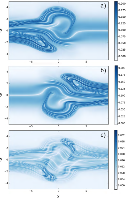
Figure 1: Values of the FTLE at each initial location ${\bf x}_{0}$, for $t_{0}=0$ and $\tau=6T$. a) Forward integration (i.e. $\lambda({\bf x}_{0},t_{0},\tau)$); large values occur at the stable manifold of the chaotic saddle. b) Backward integration (i.e. $\lambda({\bf x}_{0},t_{0},-\tau$); large values occur at the unstable manifold of the chaotic saddle. c) The product $\lambda({\bf x}_{0},t_{0},\tau)\lambda({\bf x}_{0},t_{0},-\tau)$, which is large on the chaotic saddle.

Figure 1 displays the values of the FTLE, for $t_{0}=0$, $\tau=6T$, and ${\bf x}_{0}$ on a grid of spacing $0.01\times 0.01$. The computation has been done by following all trajectories for the full interval $\tau$ without taking into account whether they remain inside $D$ or rather they leave the domain. As expected, despite the information on the escape is not explicitly taken into account, large values of he FTLE identify filamental structures that reveal the locations of the stable (top) and unstable (middle) manifolds (compare with Fig. 1b of Ref. hernandez2004sustained ). Bottom panel displays the product of forward and backwards FTLE, $\lambda({\bf x}_{0},t_{0};\tau)\lambda({\bf x}_{0},t_{0};-\tau)$, which takes large values at the intersection of the two manifolds, and then reveals the location of the chaotic saddle. We note that, for this particular flow, determining the saddle and their unstable and stable manifolds by the standard method Tel2006 ; Lai2011 of plotting the locations of the nonescaping particles at the middle, final, and initial times is rather inaccurate. The reason is the nearly vanishing velocity field at points with $|y|/l$ not close to the center of the jet ($y=0$), say $|y|\gtrsim 3$. Trajectories started at these points will finally escape the system, but only after unpractically long integration times $\tau$. The FTLE computation, however, clearly distinguishes the saddle and manifold regions because of their large finite-time stretching effect on the fluid elements.

IV.2 Network construction and analysis

To construct the flow network, we discretize $D$ into $N=180\times 100=18000$ boxes of size $0.1\times 0.1$. We release initially (taking $t_{0}=0$) 100 particles inside each box and compute their final position after a time $\tau=6T=37.699$. By counting the particles interchanged between each pair of boxes we compute $\mathbf{P}(t_{0},\tau)$ and the associated matrices $\mathbf{A}(t_{0})$ and $\mathbf{Q}(t_{0},\tau)$ (and $\mathbf{Q}^{B}(t_{0},\tau)$), from which we calculate the different network-node properties defined above. Because of the escaping particles, $S_{O}(i)<1$ in most nodes. The exception are many nodes in $|y|\gtrsim 3$ for which, as stated above, the velocities are so small that particles remain essentially immobile. An estimation of the escape rate excluding this region, and thus characteristic of the saddle, is $\kappa(D,t_{0};\tau)\approx 0.03\pm 0.01$ so that the residence time is of the order of 33.33, or approximately $5~{}T$.

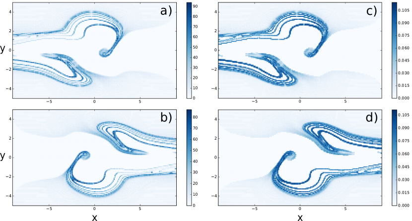
Figure 2: Network quantifiers at the different nodes, giving a coarse-grained description of the dynamical structures in the flow. a) Out-degree $K_{O}(i)$. b) In-degree $K_{I}(i)$. c) Forward finite-time entropy $H_{i}^{1}(t_{0},\tau)$. d) Backward finite-time entropy $H_{i}^{1}(t_{0},-\tau)$. The upper panels highlight the stable manifold of the saddle, and the lower ones its unstable manifold.

Figure 2 shows the degrees $K_{O}(i)$ and $K_{I}(i)$ (left) and the network entropies $H_{i}^{1}(t_{0},\tau)$ and $H_{i}^{1}(t_{0},-\tau)$ (right). The figures confirm that high values of these quantities identify the stable and unstable manifolds of the non-escaping set, as revealed by the Lyapunov fields in Fig. 1.

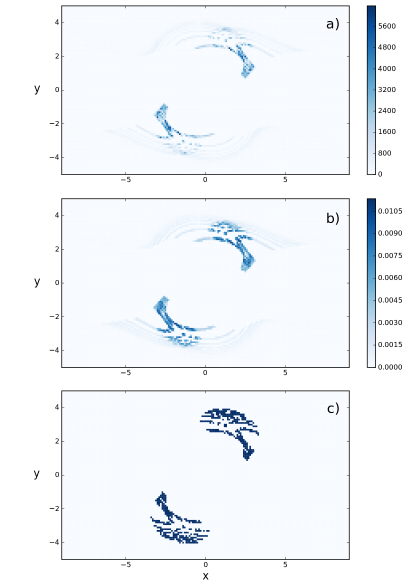
Figure 3: Three network quantifiers giving a coarse-grained identification of the chaotic saddle. a) Values of the degree product $K_{O}(i)K_{I}(i)$. b) Values of the entropy product $H_{i}^{1}(t_{0},\tau)H_{i}^{1}(t_{0},-\tau)$. c) Nodes with non-vanishing values of the cyclic clustering coefficient $C_{i}^{c}$.

Figure 3 shows three ways in which the network approach locates a coarse-grained approximation to the saddle, to be compared with the bottom panel of Fig. 1. Top panel is the product $K_{O}(i)K_{I}(i)$, and middle panel is the product $H_{i}^{1}(t_{0},\tau)~{}H_{i}^{1}(t_{0},-\tau)$. As expected, these quantities take large values at the nodes that contain the large values in Fig. 1c, i.e. nodes containing pieces of the chaotic saddle. The bottom panel in Fig. 3 shows the nodes with non-zero values of the cyclic clustering coefficient $C^{c}_{i}$. They are rodriguez2017clustering the nodes containing at time $t_{0}$ periodic trajectories of period $3\tau=18T$, which can only be present in this open system if embedded in the saddle. Because of the large period $18T$ involved, and to the finite width of the node boxes, these nodes cover indeed most of the chaotic saddle, as seen when comparing to panels a) and b) of Fig. 3 and to Fig. 1c).

V Conclusions

We have presented some numerical results, based on a simple open flow model, on the description of dynamical properties of advection by chaotic open flows within the framework of Lagrangian Flow Networks. The network approach provides a coarse-grained version of transport, and we expected that the association of network nodes with high values of degree and entropy to locations with high FTLE values, established previously for closed flows, will remain valid at least qualitatively for open flows. In particular, nodes with high values of the out-degree $K_{O}(i)$ and of the forward finite-time entropy $H_{i}^{1}(t_{0},\tau)$ will give a coarse-grained identification of the saddle and its stable manifold, whereas nodes with large in-degree $K_{I}(i)$ and backward finite-time entropy $H_{i}^{1}(t_{0},-\tau)$ will highlight the saddle and its unstable manifold. Non-vanishing values of the cyclic clustering coefficient are to be found on periodic orbits embedded on the saddle itself. We have numerically checked these expectations and then confirmed that the Lagrangian Flow Network methodology is a suitable framework to characterize finite-time and coarse-grained view of transport even for open flows with non-ideal characteristics.

As in the case of closed flows, we can not claim here that the network approach is superior in all aspects to more specific dynamical system tools. For example, Lyapunov-exponent techniques for coherent structures were available haller2000lagrangian ; shadden2005definition ; haller2015lagrangian before its reformulation in terms of networks sergiacomi2015flow , specific algorithms to find periodic orbits in dynamical systems are well developed Nayfeh1995 , as well as techniques to deal with open systems Lai2011 . Usually the network approach requires shorter trajectory integration, but this advantage is compensated by the need to use many initial conditions to cover the full domain. What is interesting in the network approach is that it provides alternatives to all these sets of techniques within a single framework, that the coarse-graining step automatically tests for robustness to noise or diffusion, and that it allows the use of techniques, such as community detection or path-finding algorithms sergiacomi2015flow ; sergiacomi2015most ; sergiacomi2015dominant , beyond the scope of standard dynamical-systems approaches. Future work will focus on the theoretical justification of our heuristically derived and numerically confirmed relationships, and in the development of additional network indicators more specifically designed to describe open flows.

References

- (1) J. Ottino, The Kinematics of Mixing: Stretching, Chaos, and Transport (Cambridge University Press, Cambridge, 1989)
- (2) S. Wiggins, Chaotic Transport in Dynamical Systems (Springer-Verlag, New York, 1992)
- (3) T. Tél, M. Gruiz, Chaotic dynamics: An introduction based on classical mechanics (Cambridge Univ. Press, Cambridge, 2006)
- (4) M. Cencini, F. Cecconi, A. Vulpiani, Chaos: From simple models to complex systems (World Scientific, Singapore, 2010)
- (5) A.M. Mancho, D. Small, S. Wiggins, Physics Reports 437, 55 (2006)
- (6) M. Cencini, G. Lacorata, A. Vulpiani, E. Zambianchi, J. Phys. Oceanogr. 29(10), 2578 (1999)
- (7) A. Bracco, J.H. LaCasce, A. Provenzale, J. Phys. Oceanogr. 30(3), 461 (2000)
- (8) J. Lacasce, Progress in Oceanography 77, 1 (2008)
- (9) A. Martin, Progress in Oceanography 57, 125 (2003)
- (10) M. Sandulescu, E. Hernández-García, C. López, U. Feudel, Tellus A 58, 605 (2006)
- (11) M. Sandulescu, E. Hernández-García, C. López, U. Feudel, Nonlinear Process. Geophys. 14, 443 (2007)
- (12) M. Sandulescu, C. López, E. Hernández-García, U. Feudel, Ecological Complexity 5, 228 (2008)
- (13) F. d’Ovidio, V. Fernández, E. Hernandez-García, C. López, Geophys. Res. Lett. 31, L17203 (2004)
- (14) T. Peacock, J. Dabiri, Chaos 20, 017501 ( 3) (2010)
- (15) J. Bettencourt, C. López, E. Hernández-García, Ocean Modell. 51, 73 (2012)
- (16) A. Barrat, M. Barthelemy, A. Vespignani, Dynamical processes on complex networks (Cambridge Univ Press, Cambridge, 2008)
- (17) M.E.J. Newman, Networks: An Introduction. (Oxford University Press, Oxford, 2010), ISBN 978-0-19-920665-0
- (18) J.F. Donges, Y. Zou, N. Marwan, J. Kurths, The European Physical Journal-Special Topics 174, 157 (2009)
- (19) E. Ser-Giacomi, V. Rossi, C. López, E. Hernández-García, Chaos 25, 036404 (2015)
- (20) E. Ser-Giacomi, R. Vasile, E. Hernández-García, C. López, Physical Review E 92, 012818 (2014)
- (21) E. Ser-Giacomi, R. Vasile, I. Recuerda, E. Hernández-García, C. López, Chaos 25, 087413 (2015)
- (22) M. Lindner, R. Donner, Chaos 27, 035806 (2017)
- (23) V. Rodríguez-Méndez, E. Ser-Giacomi, E. Hernández-García, Chaos 27, 035803 (2017)
- (24) G. Froyland, M. Dellnitz, SIAM Journal on Scientific Computing 24, 1839 (2003)
- (25) G. Froyland, Physica D: Nonlinear Phenomena 200, 205 (2005)
- (26) G. Froyland, K. Padberg, M.H. England, A.M. Treguier, Physical Review Letters 98, 224503 (2007)
- (27) M.K. Singh, T.G. Kang, H.E.H. Meijer, P.D. Anderson, Microfluidics and Nanofluidics 5, 313 (2008)
- (28) M. Dellnitz, G. Froyland, C. Horenkamp, K. Padberg-Gehle, A. Sen Gupta, Nonlinear Processes in Geophysics 16, 655 (2009)
- (29) G. Froyland, C. Horenkamp, V. Rossi, N. Santitissadeekorn, A.S. Gupta, Ocean Modelling 52, 69 (2012)
- (30) P. Tallapragada, S.D. Ross, Communications in Nonlinear Science and Numerical Simulation 18, 1106 (2013)
- (31) E.M. Bollt, N. Santitissadeekorn, Applied and Computational Measurable Dynamics (SIAM, Philadelphia, 2013)
- (32) V. Rossi, E. Ser-Giacomi, C. López, E. Hernández-García, Geophysical Research Letters 41, 2883 (2014)
- (33) Y. Lai, T. Tél, Transient Chaos: Complex Dynamics on Finite-Time Scales (Springer, 2011)
- (34) E. Ott, Chaos in Dynamical Systems (Cambridge Univ. Press, Cambridge (UK), 1993)
- (35) S.C. Shadden, F. Lekien, J.E. Marsden, Physica D 212, 271 (2005)
- (36) G. Haller, G. Yuan, Physica D 147, 352 (2000)
- (37) S.C. Shadden, F. Lekien, J.E. Marsden, Physica D 212, 271 (2005)
- (38) G. Haller, Annual Review of Fluid Mechanics 47, 137 (2015)
- (39) G. Froyland, K. Padberg-Gehle, Physica D: Nonlinear Phenomena 241, 1612 (2012)
- (40) M.E.J. Newman, SIAM Review 45, 167 (2003)
- (41) M. Newman, Networks: An introduction (Oxford University Press, 2009)
- (42) J. Saramäki, M. Kivelä, J.P. Onnela, K. Kaski, J. Kertész, Phys. Rev. E 75, 027105 (2007)
- (43) G. Fagiolo, Phys. Rev. E 76, 026107 (2007)
- (44) R. Milo, S. Shen-Orr, S. Itzkovitz, N. Kashtan, D. Chklovskii, U. Alon, Science 298, 824 (2002)
- (45) G. Froyland, R.M. Stuart, E. van Sebille, Chaos: An Interdisciplinary Journal of Nonlinear Science 24, 033126 (2014)
- (46) E. Hernández-García, C. López, Ecological Complexity 1, 253 (2004)
- (47) A. H. Nayfeh and B. Balachandran, Applied Nonlinear Dynamics: Analytical, Computational and Experimental Methods (John Wiley, New York, 1995)