Estimating the Critical Parameters of the Hard Square Lattice Gas Model

Abstract

The hard square lattice gas model on a square lattice is known to undergo a continuous phase transition from a low density fluid-like phase to high density phase with columnar or smectic order. We estimate the critical activity $z_{c}$ by calculating, within an approximation scheme, the interfacial tension between two differently ordered columnar phases, and then setting it to zero. The approximation scheme allows for the ordered phases to have multiple defects and the interface between the ordered phases to have overhangs. We estimate $z_{c}=105.35$, which is in good agreement with existing Monte Carlo simulation results of $z_{c}\approx 97.5$, and is an improvement over earlier best estimates of $z_{c}=54.87$ and $z_{c}=135.63$.

1 Introduction

The study of entropy driven transitions in the $2\times 2$ hard square lattice gas model, or equivalently the 2-NN model in which a particle excludes the nearest and next-nearest neighbor from being occupied by another particle, has a long history dating back to the 1950s [1, 2, 3, 4, 5, 6, 7]. The hard square model is known to undergo a continuous transition from a disordered fluid-like phase to an ordered phase with columnar order as the density $\rho$ or activity $z$ is increased. The best numerical estimates for the critical behavior, obtained from large scale Monte Carlo simulations, are critical activity $z_{c}\approx 97.5$, critical density $\rho_{c}\approx 0.932$, and critical exponents belonging to the Ashkin Teller universality class with critical exponents $\nu\approx 0.92$, $\beta/\nu=1/8$ and $\gamma/\nu=7/4$ [8, 9, 10, 11]. Unlike the hard hexagon model [12], the hard square model is not exactly solvable. Different analytic and rigorous methods have been used to estimate the critical parameters over the last few decades [2, 13, 14, 15, 16, 17, 18, 19, 20]. The estimates for $z_{c}$ and $\rho_{c}$ obtained from different methods are summarized in table 1. Analytical approaches like high density expansion [2, 14], Flory-type approximations [19], density functional theory [15, 16], etc., result in estimates that underestimate the critical activity by more than a factor of 7. Calculations based on estimating the interfacial tension [17, 18] between two ordered phases have been more successful. By utilizing the mapping of the hard square model to the antiferromagnetic Ising model with next nearest neighbor interactions, a fairly good estimate $z_{c}=135.63$, that overestimates the critical activity, was obtained, but it is not clear how this approach may be extended [17]. In a recent paper [18], we introduced a systematic way of determining the interfacial tension as an expansion in number of defects in the perfectly ordered phase. While including a single defect improves the estimates for the critical parameters ($z_{c}=52.49$), the calculation of the two-defect contribution appears to be too difficult to carry out. We also estimated the effect of introducing overhangs of height one in the interface for defect-free phases ($z_{c}=54.87$). However, it is not clear how defects and overhangs may be combined in a single calculation. In this paper, we determine the interfacial tension using a pairwise approximation, similar to that used in liquid state theory. This approximation scheme allows us to take into account multiple defects as well as overhangs. By determining the activity at which this interfacial tension vanishes, we estimate $z_{c}=105.35$, in reasonable agreement with numerical results ($z_{c}\approx 97.5$), and which is a significant improvement over earlier estimates.

Table 1: Estimates of critical activity $z_{c}$ and critical density $\rho_{c}$ for columnar-disordered transition of hard square model

• $z_{c}$	$\rho_{c}$	Method Used
  97.50	0.932	Numerical [8, 9, 10, 11]
  6.25	0.64	High density expansion (order one) [2, 14]
  11.09	0.76	Flory type mean field [19]
  11.09	0.76	Approximate counting [20]
  11.13	0.764	Density Functional theory [15, 16]
  14.86	0.754	High density expansion (order two) [14]
  17.22	0.807	Rushbrooke Scoins approximation [2]
  48.25	0.928	Interfacial tension with no defect [18]
  52.49	0.923	Interfacial tension with one defect [18]
  54.87	0.9326	Interfacial tension with overhang [18]
  135.63	-	Interfacial tension in anteferromagnetic Ising model [17]
  105.35	0.947	In this paper

The hard square model on the square lattice has been studied in different contexts. It is the prototypical model to study phases with columnar, smectic or layered order in which translational invariance in broken in some but not all the directions. Examples of systems showing such ordered phases include liquid crystals [21], adsorbed atoms or molecules on metal surfaces [22, 23, 24, 25, 26], etc. Columnar phases have also been of recent interest in different hard core lattice gas models. The hard rectangle gas shows a nematic-columnar phase transition, in addition to isotropic-nematic and columnar-sublattice transitions [27, 28]. Of these, in the limit of infinite aspect ratio, only the nematic-columnar transition survives at a finite packing density [29, 30]. Generalized models consisting of a mixture of hard squares and dimers [9] or interacting dimers [31] also show a columnar phase. The presence of a columnar phase has also been shown to result in the $k$-NN model, in which the excluded volume of a particle is made up of its first $k$ next nearest neighbors, undergoing multiple entropy driven phase transitions with increasing density [32, 33]. The study of columnar phases has also been of recent interest in quantum spin systems [34, 35, 36, 37, 11]. The hard square system has also found application in modeling adsorption [23, 22], in combinatorial problems and tilings [38, 39, 40], and has been the the subject of recent direct experiments [41, 42].

The remainder of the paper is organized as follows. In section 2, we define the model precisely and outline the steps in the calculation of the interfacial tension between two ordered columnar phases. The calculation involves determining the eigenvalue of a transfer matrix $T$, which is computed in section 3. In section 4 the different quantities determining the largest eigenvalue of $T$ are computed by calculating exactly the partition function of hard squares on tracks made up of 2 and 4 rows with appropriate boundary conditions. The results for the interfacial tension are obtained in section 5. We end with a summary and discussion in section 6.

2 Model and Outline of Calculation

Consider a square lattice of size $N_{x}$ $\times$ $N_{y}$. The sites may be occupied by particles that are hard squares of size $2\times 2$. The squares interact through only excluded volume interaction i.e. two squares can not overlap but may touch each other. We associate an activity $z$ to each square.

At low activities $z$ or equivalently at low densities $\rho$, the system is in a disordered phase. For activities larger than critical value $z_{c}$, the system is in a broken-symmetry phase with columnar order, which we define more precisely below. Let the lower left corner of a square be denoted as its head. In the columnar phase, the heads preferentially occupy even or odd rows with all columns being equally occupied, or preferentially occupy even or odd columns with all rows being equally occupied. An example of a row-ordered phase is shown in figure 1. The snapshot of a equilibrated configuration is shown in two different representations. When the squares are colored according to whether their heads are in even or odd rows [see figure 1(a)], one color is predominantly seen. However, when the same configuration is colored according to whether the heads of the squares are in even or odd columns [see figure 1(b)], then both colors appear in roughly equal proportion. There are clearly $4$ ordered phases possible.

Figure 1: Snapshot of a equilibrated configuration of system of hard squares with activity $z=110.0$, corresponding $\rho\approx 0.937$. These parameters correspond to the system being in an ordered phase. A square is colored blue or green depending on whether its head (bottom left point) is in even or odd (a) row and (b) column. The dominance of one color in (a) implies that the system is a row-ordered phase. The snapshot was generated using Monte Carlo simulation using the cluster algorithm introduced in [43, 44].

The aim of this paper is to estimate the critical activity $z_{c}$ and critical density $\rho_{c}$ separating the disordered phase from the ordered columnar phase. To do so, we determine, within an approximation scheme, the interfacial tension $\sigma(z)$ between two differently ordered columnar phase and equate it to zero to obtain the transition point. Consider boundary conditions where the left edge of the square lattice is fixed to the occupied by squares with heads in even row and the right edge is fixed to be occupied by squares in odd row. For large $z$, this choice of boundary condition ensures that there is an interface running from top to bottom separating a left phase or domain constituted of squares predominantly in even rows from a right phase or domain constituted of squares predominantly in odd rows. A schematic diagram of the interface is shown in figure 2. We will refer to the two phases as left and right phases or domains from now on. Let $Z^{(0)}$ be the partition functions of the system without an interface and $Z^{(\mathcal{I})}$ be the partition function when an interface $\mathcal{I}$ is present. The interfacial tension $\sigma(z)$ is defined as

$$e^{-\sigma N_{y}}=\frac{\sum_{\mathcal{I}}Z^{(\mathcal{I})}}{Z^{(0)}}.$$ (1)

As the interactions between the squares are only excluded volume interactions, the partition function in the presence of an interface may be written as a product of partition function of the left and right phases, i.e.

$$Z^{(\mathcal{I})}=Z^{(\mathcal{I})}_{L}Z^{(\mathcal{I})}_{R},$$ (2)

where $Z^{(\mathcal{I})}_{L}$ and $Z^{(\mathcal{I})}_{R}$ denote the partition functions of the left and right phases in the presence of an interface $\mathcal{I}$. It is not possible to determine $Z^{(\mathcal{I})}_{L}$, $Z^{(\mathcal{I})}_{R}$ or $Z^{(0)}$ exactly. In what follows, we calculate these partition functions within certain approximations.

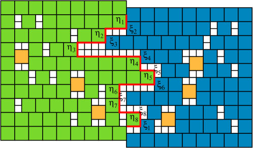
Figure 2: Schematic diagram of a configuration in the presence of an interface. The boundary conditions are such that the left (right) edge of the square is fixed to be occupied by even (odd) squares. The interface, constituted of the right edges of the right-most squares of the left domain is denoted by the red line and labeled by $\eta_{i}$. $\xi_{i}$ denotes the left-most position possible for a square belonging to the right domain.

First, we assume that the interface between the left and right phases is a directed walk from top to bottom, ie the interface does not have any upward steps. We define the position of the interface to be the right boundary of the rightmost squares of the left phase. The interface is denoted by $\eta_{i}$ as shown in figure 2. We also define $\xi_{i}$ to the left most position that a square in the right phase may occupy on row $i$, as shown in figure 2. Clearly,

$$\xi_{i}=\max(\eta_{i-1},\eta_{i}),\quad i=1,2,..,N_{y}/2.$$ (3)

Given an interface, we compute the partition function within an approximation. The simplest approximation is it to write the partition function as a product of partition functions of tracks of width two, corresponding to two consecutive rows. This approximation has the drawback that the ordered left and right phases do not have any defects, where the squares of wrong type i.e. odd squares in left or even phase and even squares in the right or odd phase will be called defects (denoted by yellow in figure 2). The calculation of interfacial tension then reduces to the special case of zero-defects of [18]. The simplest approximation that allows defects to be present is the pairwise approximation, where the partition function is written as a product of $N_{y}/2$ partition functions of tracks of width four, made up of four consecutive rows. We write

$$Z^{(\mathcal{I})}_{L} = \frac{\omega_{2}^{(L)}(\eta_{1},\eta_{2})\omega_{2}^{(L)}(\eta_{2},\eta_{3})~{}...~{}\omega_{2}^{(L)}(\eta_{N_{y}/2},\eta_{1})}{\mathcal{L}^{(L)}(\eta_{1})\mathcal{L}^{(L)}(\eta_{2})~{}...~{}\mathcal{L}^{(L)}(\eta_{N_{y}/2})},$$ (4)

$$Z^{(\mathcal{I})}_{R} = \frac{\omega_{2}^{(R)}(N_{x}-\xi_{1},N_{x}-\xi_{2})~{}...~{}\omega_{2}^{(R)}(N_{x}-\xi_{N_{y}/2},N_{x}-\xi_{1})}{\mathcal{L}^{(R)}(N_{x}-\xi_{1})~{}...~{}\mathcal{L}^{(R)}(N_{x}-\xi_{N_{y}/2})},$$ (5)

$$Z^{(0)} = \frac{{[\omega_{2}(N_{x},N_{x})]}^{N_{y}/2}}{{[\mathcal{L}(N_{x})]}^{N_{y}/2}},$$ (6)

where $\omega_{2}(\ell_{1},\ell_{2})$ is the partition function of a track of width $4$ where first two rows are of length $\ell_{1}$ and third and fourth rows of length $\ell_{2}$, and $\mathcal{L}(\ell)$ is the partition function of a track of width $2$ where both rows have length $\ell$. The superscripts $(L)$ and $(R)$ denote left and right phases. The choice of the denominator is motivated by the fact that in the absence of defects, $\omega_{2}(\ell_{1},\ell_{2})=\mathcal{L}(\ell_{1})\mathcal{L}(\ell_{2})$. In this case, the overall partition function should reduce to a product over $\mathcal{L}$’s, and the choice of the denominator ensures this.

The partition functions for the left and right phases are different, and also not the same as the partition function of the system without an interface, because the presence of the interface imposes introduces constraints on the positioning of squares near the interface. The constraints are as follows. For the left partition function $\omega_{2}^{(L)}(\ell_{1},\ell_{2})$, there must be even squares (non-defects) present whose right edges are aligned with the position of the interface in both sets of two rows each corresponding to $\ell_{1}$ and $\ell_{2}$. This is because the position of the interface has been defined as the right edge of the rightmost square of the left phase. For the right partition function $\omega_{2}^{(L)}(\ell_{1},\ell_{2})$, the constraint is that there must at least one odd square (non-defect) between the interface and the left-most defect square. Otherwise, the interface can be redefined to include the defect square into the left phase. In addition, there is the question of whether defects can be placed between $\ell_{1}$ and $\ell_{2}$ for the left and right phases. Placing defects here is equivalent to allowing the interface to have overhangs. To prevent overcounting, we will disallow such defects for the left phase, but allow them for the right phase. Equivalently, a defect in the left phase may be placed only in the region to the left of $\min(\ell_{1},\ell_{2})$, and a defect in the right phase can be placed to the right of $\min(N_{x}-\ell_{1},N_{x}-\ell_{2})$.

It is convenient to shift to a notation where (see figure 3)

$$\omega_{2}(\ell_{1},\ell_{2})=\Omega_{2}\big{[}\min(\ell_{1},\ell_{2}),|\ell_{1}-\ell_{2}|\big{]}$$ (7)

Then, the partition function $Z^{(L)}$, $Z^{(R)}$ and $Z^{(0)}$ may be rewritten as

$$Z^{(\mathcal{I})}_{L} = \frac{\prod_{i=1}^{N_{y}/2}\Omega_{2}^{(L)}\big{[}\min(\eta_{i},\eta_{i+1}),|\eta_{i}-\eta_{i+1}|\big{]}}{\prod_{i=1}^{N_{y}/2}\mathcal{L}^{(L)}(\eta_{i})},$$ (8)

$$Z^{(\mathcal{I})}_{R} = \frac{\prod_{i=1}^{N_{y}/2}\Omega_{2}^{(R)}\big{[}N_{x}-\max(\xi_{i},\xi_{i+1}),|\xi_{i}-\xi_{i+1}|\big{]}}{\prod_{i=1}^{N_{y}/2}\mathcal{L}^{(R)}(N_{x}-\xi_{i})},$$ (9)

$$Z^{(0)} = \frac{{[\Omega_{2}(N_{x},0)]}^{N_{y}/2}}{{[\mathcal{L}(N_{x})]}^{N_{y}/2}},$$ (10)

For large $\ell$, the partition functions $\Omega_{2}$ and $\mathcal{L}$ diverge exponentially with the system size. We define

$$\Omega_{2}(\ell,\Delta) = a_{2}(\Delta)\lambda_{2}^{2\ell+\Delta},$$ (11)

$$\Omega_{2}^{(L)}(\ell,\Delta) = a_{2}^{(L)}(\Delta)\lambda_{2}^{2\ell+\Delta},\quad\ell\gg 1,$$ (12)

$$\Omega_{2}^{(R)}(\ell,\Delta) = a_{2}^{(R)}(\Delta)\lambda_{2}^{2\ell+\Delta},$$ (13)

and

$$\mathcal{L}(\ell) = a_{1}\lambda_{1}^{\ell},$$ (14)

$$\mathcal{L}^{(L)}(\ell) = a_{1}^{(L)}\lambda_{1}^{\ell},\quad\ell\gg 1,$$ (15)

$$\mathcal{L}^{(R)}(\ell) = a_{1}^{(R)}\lambda_{1}^{\ell}.$$ (16)

Note that we have used the same exponential factor for all $\Omega_{2}$ (as well as for all $\mathcal{L}$), since the free energy is independent of constraints arising from the boundary conditions. It is easy to determine $a_{1}^{(L)}$ and $a_{1}^{(R)}$ in terms of $a_{1}$. In the left domain, for a track of width 2, the constraint is that the rightmost square must touch the interface. This means that $\mathcal{L}^{(L)}(\ell)=z\mathcal{L}(\ell-2)\approx za_{1}\lambda_{1}^{\ell-2}$. In the right domain, defects cannot be present in a track of width 2, and hence there are no constraints, implying that $\mathcal{L}^{(R)}(\ell)=\mathcal{L}(\ell)\approx a_{1}\lambda_{1}^{\ell}$. Therefore,

$$a_{1}^{(L)} = \frac{za_{1}}{\lambda_{1}^{2}},$$ (17)

$$a_{1}^{(R)} = a_{1}.$$ (18)

Figure 3: Schematic diagram of a (a) track of width $4$ (four rows) with partition function $\Omega_{2}(\ell,\Delta)$ and (b) track of width $2$ (two rows) with partition function $\mathcal{L}(\ell)$.

Using the asymptotic forms for the partition functions, the partition functions of the left [see (8)] and right [see (9)] phases may be rewritten as

$$Z^{(\mathcal{I})}_{L} = \frac{\prod_{i=1}^{N_{y}/2}a_{2}^{(L)}\big{(}|\eta_{i}-\eta_{i+1}|\big{)}\lambda_{2}^{2\min(\eta_{i},\eta_{i+1})+|\eta_{i}-\eta_{i+1}|}}{\prod_{i=1}^{N_{y}/2}za_{1}\lambda_{1}^{\eta_{i}-2}},$$ (19)

$$Z^{(\mathcal{I})}_{R} = \frac{\prod_{i=1}^{N_{y}/2}a_{2}^{(R)}\big{(}|\xi_{i}-\xi_{i+1}|\big{)}\lambda_{2}^{2N_{x}-2\max(\xi_{i},\xi_{i+1})+|\xi_{i}-\xi_{i+1}|}}{\prod_{i=1}^{N_{y}/2}a_{1}\lambda_{1}^{N_{x}-\xi_{i}}}.$$ (20)

Using the relations $2\min(m,n)=m+n-|m-n|$ and $2\max(m,n)=m+n+|m-n|$, taking product of $Z^{(L)}$ and $Z^{(R)}$ and simplifying, we obtain

$$Z^{(\mathcal{I})}=\frac{\lambda_{2}^{N_{x}N_{y}}\prod_{i=1}^{N_{y}/2}a_{2}^{(L)}\big{(}|\eta_{i}-\eta_{i+1}|\big{)}a_{2}^{(R)}\big{(}|\xi_{i}-\xi_{i+1}|\big{)}\lambda_{2}^{-|\eta_{i}-\eta_{i+1}|}}{{\bigg{(}\frac{za_{1}^{2}}{\lambda_{1}^{2}}\bigg{)}}^{N_{y}/2}\lambda_{1}^{N_{x}N_{y}/2}\prod_{i=1}^{N_{y}/2}\lambda_{1}^{-\frac{1}{2}|\eta_{i}-\eta_{i+1}|}}.$$ (21)

Likewise, the partition function of the system without an interface [see (10)] may be written for large $N_{x}$ as

$$Z^{(0)}={\bigg{[}\frac{a_{2}(0)\lambda_{2}^{2N_{x}}}{a_{1}\lambda_{1}^{N_{x}}}\bigg{]}}^{N_{y}/2}.$$ (22)

Knowing the partition functions (21) and (22), the interfacial tension in (1) may be expressed in terms of $a$’s, $\lambda_{1}$ and $\lambda_{2}$ as

$$e^{-\sigma N_{y}}={\bigg{[}\frac{\lambda_{1}^{2}}{za_{1}a_{2}(0)}\bigg{]}}^{N_{y}/2}\sum_{\mathcal{I}}\prod_{i=1}^{N_{y}/2}\frac{a_{2}^{(L)}\big{(}|\eta_{i}-\eta_{i+1}|\big{)}a_{2}^{(R)}\big{(}|\xi_{i}-\xi_{i+1}|\big{)}\lambda_{2}^{-|\eta_{i}-\eta_{i+1}|}}{\lambda_{1}^{-\frac{1}{2}|\eta_{i}-\eta_{i+1}|}}.$$ (23)

We note that all arguments are in terms of differences between consecutive $\eta_{i}$’s or $\xi_{i}$’s. It is therefore convenient to introduce new variables

$${\widetilde{\eta}}_{i}=\eta_{i}-\eta_{i-1}.$$ (24)

In terms of these new variables, it is straightforward to derive

$$\xi_{i+1}-\xi_{i}={\widetilde{\eta}}_{i+1}\theta({\widetilde{\eta}}_{i+1})+{\widetilde{\eta}}_{i}(1-\theta({\widetilde{\eta}}_{i})),$$ (25)

where $\theta(x)$ is the Heaviside step function defined as $\theta(x)=1$ for $x\geq 0$ and $\theta(x)=0$ for $x<0$. In terms of these new variables ${\widetilde{\eta}}_{i}$, the interfacial tension (23) may be rewritten as

$$e^{-\sigma N_{y}}={\bigg{[}\frac{\lambda_{1}^{2}}{za_{1}a_{2}(0)}\bigg{]}}^{N_{y}/2}\sum_{[{\widetilde{\eta}}_{i}]}\prod_{i=1}^{N_{y}/2} {\bigg{(}\frac{\sqrt{\lambda_{1}}}{\lambda_{2}}\bigg{)}}^{|{\widetilde{\eta}}_{i}|}a_{2}^{(L)}\big{(}|{\widetilde{\eta}}_{i}|\big{)}\times$$ (26)

$$a_{2}^{(R)}\big{(}|{\widetilde{\eta}}_{i+1}\theta({\widetilde{\eta}}_{i+1})+{\widetilde{\eta}}_{i}(1-\theta({\widetilde{\eta}}_{i}))|\big{)},$$

where the sum over ${\widetilde{\eta}}_{i}$ varies from $-\infty$ to $+\infty$.

The summation over ${\widetilde{\eta}}_{i}$ is not straightforward to do as they are not independent due to terms coupling ${\widetilde{\eta}}_{i}$ and ${\widetilde{\eta}}_{i+1}$. To do the sum, we define an infinite dimensional transfer matrix $T$ with coefficients

$$T_{{\widetilde{\eta}}_{i},{\widetilde{\eta}}_{i+1}}={\bigg{(}\frac{\sqrt{\lambda_{1}}}{\lambda_{2}}\bigg{)}}^{|{\widetilde{\eta}}_{i}|}a_{2}^{(L)}\big{(}|{\widetilde{\eta}}_{i}|\big{)}a_{2}^{(R)}\big{(}|{\widetilde{\eta}}_{i+1}\theta({\widetilde{\eta}}_{i+1})+{\widetilde{\eta}}_{i}(1-\theta({\widetilde{\eta}}_{i}))|\big{)}.$$ (27)

Let $\Lambda_{2}$ be the largest eigenvalue of the transfer matrix $T$. For large $N_{y}$, we may then write (26) as

$$e^{-\sigma N_{y}}={\bigg{[}\frac{\lambda_{1}^{2}}{za_{1}a_{2}(0)}\bigg{]}}^{N_{y}/2}\sum_{[{\widetilde{\eta}}_{i}]}\prod_{i=1}^{N_{y}/2}T_{{\widetilde{\eta}}_{i},{\widetilde{\eta}}_{i+1}}={\bigg{[}\frac{\lambda_{1}^{2}\Lambda_{2}}{za_{1}a_{2}(0)}\bigg{]}}^{N_{y}/2}.$$ (28)

At the transition point, $\sigma$ vanishes, and the critical activity $z_{c}$ therefore satisfies the relation

$$\frac{\lambda_{1}^{2}\Lambda_{2}}{z_{c}a_{1}a_{2}(0)}=1,$$ (29)

where $\Lambda_{2}$ depends on $a_{2}^{(R)}$ and $a_{2}^{(L)}$. These unknown parameters are calculated exactly in section 3 and section 4.

3 Calculation of Eigenvalue of $T$

In this section, we determine the largest eigenvalue of the transfer matrix $T$ with components as defined in (27). Let the largest eigenvalue of $T$ be denoted by $\Lambda_{2}$ corresponding to an eigenvector $\Psi$ with components $\psi_{i}$, $i=-\infty,\ldots,\infty$. In component form, the eigenvalue equation is

$$\sum_{j=-\infty}^{\infty}T_{i,j}\psi_{j}=\Lambda_{2}\psi_{i},~{}i=-\infty,\ldots,\infty.$$ (30)

Substituting for $T$ from (27), we obtain

$$\bigg{(}\frac{\sqrt{\lambda_{1}}}{\lambda_{2}}\bigg{)}^{|i|}a_{2}^{(L)}(|i|)\bigg{[}a_{2}^{(R)}(0)\sum_{j=-\infty}^{0}\psi_{j}+\sum_{j=1}^{\infty}a_{2}^{(R)}(|j|)\psi_{j}\bigg{]}\\ =\Lambda_{2}\psi_{i},~{}i\geq 0,$$ (31)

$$\bigg{(}\frac{\sqrt{\lambda_{1}}}{\lambda_{2}}\bigg{)}^{|i|}a_{2}^{(L)}(|i|)\bigg{[}a_{2}^{(R)}(|i|)\sum_{j=-\infty}^{0}\psi_{j}+\sum_{j=1}^{\infty}a_{2}^{(R)}(|j+i|)\psi_{j}\bigg{]}\\ =\Lambda_{2}\psi_{i},~{}i<0.$$ (32)

First consider the case for $i\geq 0$. Equation (31) may be re-written as

$$\bigg{(}\frac{\sqrt{\lambda_{1}}}{\lambda_{2}}\bigg{)}^{|i|}a_{2}^{(L)}(|i|)\bigg{[}a_{2}^{(R)}(0)\beta+\sum_{j=1}^{\infty}a_{2}^{(R)}(|j|)\widetilde{\psi}_{j}\bigg{]}=\Lambda_{2}\widetilde{\psi}_{i},~{}i\geq 0,$$ (33)

where

$$\widetilde{\psi}_{i}=\frac{\psi_{i}}{\psi_{0}};~{}~{}\beta=\sum_{i=-\infty}^{0}\widetilde{\psi}_{i}.$$ (34)

Since $\widetilde{\psi}_{0}=1$, from (33) with $i=0$, we immediately obtain the eigenvalue $\Lambda_{2}$ to be

$$\Lambda_{2}=a_{2}^{(L)}(0)\left[a_{2}^{(R)}(0)\beta+\sum_{j=1}^{\infty}a_{2}^{(R)}(|j|)\widetilde{\psi}_{j}\right].$$ (35)

with components of the eigenvector being

$$\widetilde{\psi}_{i}={\bigg{(}\frac{\sqrt{\lambda_{1}}}{\lambda_{2}}\bigg{)}}^{|i|}\frac{a_{2}^{(L)}(|i|)}{a^{(L)}(0)},~{}i\geq 0.$$ (36)

Now, consider the case $i<0$. In terms of $\widetilde{\psi}_{i}$, (32) may be written as

$${\bigg{(}\frac{\sqrt{\lambda_{1}}}{\lambda_{2}}\bigg{)}}^{|i|}a_{2}^{(L)}(|i|)\bigg{[}a_{2}^{(R)}(|i|)\beta+\sum_{j=1}^{\infty}a_{2}^{(R)}(|j+i|)\widetilde{\psi}_{j}\bigg{]}=\Lambda_{2}\widetilde{\psi}_{i},~{}i<0.$$ (37)

Substituting $\widetilde{\psi}_{j}$ for $j\geq 0$, from (36), we obtain

$${\bigg{(}\frac{\sqrt{\lambda_{1}}}{\lambda_{2}}\bigg{)}}^{|i|}a_{2}^{(L)}(|i|)F(i)=\Lambda_{2}\widetilde{\psi}_{i},~{}i<0,$$ (38)

where, the function $F(i)$ is defined as

$$F(i)=a_{2}^{(R)}(|i|)\beta+\sum_{j=1}^{\infty}{\bigg{(}\frac{\sqrt{\lambda_{1}}}{\lambda_{2}}\bigg{)}}^{|j|}\frac{a_{2}^{(R)}(|j+i|)a_{2}^{(L)}(|j|)}{a_{2}^{(L)}(0)}.$$ (39)

The solution to (38) is clearly

$$\Lambda_{2}=a_{2}^{(L)}(0)F(0),$$ (40)

which is consistent with (35), and

$$\widetilde{\psi}_{i}={\bigg{(}\frac{\sqrt{\lambda_{1}}}{\lambda_{2}}\bigg{)}}^{|i|}\frac{a_{2}^{(L)}(|i|)F(i)}{a_{2}^{(L)}(0)F(0)},~{}i<0.$$ (41)

Equation (35), (36), and (41) determine $\Lambda_{2}$ and the components of the eigenvector. To solve for $\Lambda_{2}$ in terms of $a_{2}^{(L)}(\Delta)$ and $a_{2}^{(R)}(\Delta)$, it is convenient to define three quantities

$$k_{1} = \sum_{i=1}^{\infty}{\bigg{(}\frac{\sqrt{\lambda_{1}}}{\lambda_{2}}\bigg{)}}^{|i|}a_{2}^{(L)}(|i|)a_{2}^{(R)}(|i|),$$ (42)

$$k_{2} = \sum_{i=-\infty}^{0}{\bigg{(}\frac{\sqrt{\lambda_{1}}}{\lambda_{2}}\bigg{)}}^{|i|}a_{2}^{(L)}(|i|)a_{2}^{(R)}(|i|),$$ (43)

$$k_{3} = \sum_{i=-\infty}^{0}\sum_{j=1}^{\infty}{\bigg{(}\frac{\sqrt{\lambda_{1}}}{\lambda_{2}}\bigg{)}}^{|i|+|j|}\frac{a_{2}^{(L)}(|i|)a_{2}^{(R)}(|i+j|)a_{2}^{(L)}(|j|)}{a_{2}^{(L)}(0)}.$$ (44)

Solving for $\beta$ in (34) and (35) by substituting for $\widetilde{\psi}_{i}$ from (41) and (36) respectively, we obtain

$$\beta = \frac{k_{3}}{\Lambda_{2}-k_{2}},$$ (45)

$$\beta = \frac{\Lambda_{2}-k_{1}}{a_{2}^{(L)}(0)a_{2}^{(R)}(0)}.$$ (46)

Equating (45) and (46) to eliminate $\beta$, we find that $\Lambda_{2}$ satisfies the quadratic equation

$$\Lambda_{2}^{2}-(k_{1}+k_{2})\Lambda_{2}+k_{1}k_{2}-k_{3}a_{2}^{(L)}(0)a_{2}^{(R)}(0)=0,$$ (47)

whose largest root is

$$\Lambda_{2}=\frac{k_{1}+k_{2}+\sqrt{{(k_{1}-k_{2})}^{2}+4a_{2}^{(L)}(0)a_{2}^{(R)}(0)k_{3}}}{2}.$$ (48)

The largest eigenvalue may be further simplified using

$$k_{2}-k_{1} =a_{2}^{(L)}(0)a_{2}^{(R)}(0),$$ (49)

$$\widetilde{k} =k_{2}+k_{1}=\sum_{i=-\infty}^{\infty}{\bigg{(}\frac{\sqrt{\lambda_{1}}}{\lambda_{2}}\bigg{)}}^{|i|}a_{2}^{(L)}(|i|)a_{2}^{(R)}(|i|).$$ (50)

After simplification we get the largest eigenvalue

$$\Lambda_{2}=\frac{\widetilde{k}+\sqrt{{\big{[}a_{2}^{(L)}(0)a_{2}^{(R)}(0)\big{]}}^{2}+4a_{2}^{(L)}(0)a_{2}^{(R)}(0)k_{3}}}{2},$$ (51)

with $k_{3}$ as in (44) and $\widetilde{k}$ as in (50).

4 Calculation of Partition Functions of Tracks

4.1 Partition function of track of width $2$

In this section, we determine the asymptotic behavior of the partition function $\mathcal{L}(\ell)$ of a track of width $2$ and length $\ell$ [the shape of the track is shown in figure 3(b)]. We define the generating function

$$G_{1}(y)=\sum_{\ell=0}^{\infty}\mathcal{L}(\ell)y^{\ell},$$ (52)

where the power of $\sqrt{y}$ is the number of sites present in the system. The recursion relation obeyed by $G_{1}(y)$ is shown diagrammatically in figure 4 and can be written as

$$G_{1}(y)=1+yG_{1}(y)+zy^{2}G_{1}(y),$$ (53)

which may be solved to give

$$G_{1}(y)=\frac{1}{1-y-zy^{2}}.$$ (54)

Let $y_{1}$ be the smallest root of the denominator $1-y-zy^{2}$ of (54), i.e.

$$y_{1}=\frac{\sqrt{1+4z}-1}{2z}.$$ (55)

By finding the coefficient of $y^{\ell}$ for large $\ell$, it is straightforward to obtain

$$\mathcal{L}(\ell)=a_{1}\lambda_{1}^{\ell}[1+O(\exp(-c\ell))],~{}c>0,~{}\ell\gg 1,$$ (56)

where

$$\lambda_{1}=\frac{1}{y_{1}},~{}~{}a_{1}=\frac{1}{2-y_{1}}.$$ (57)

Figure 4: Diagrammatic representation of the recursion relation obeyed by the generating function $G_{1}(y)$ defined for a track of width 2 [see (52) for definition]. The first column of the track may be occupied by two vacancies (open 1$\times$1 square) or a square (filled 2$\times$2 square).

4.2 Partition functions for tracks of width $4$

In this section we determine the partition functions of tracks of width $4$ without any constraints. The shape of a generic track of width $4$ is characterized by parameters $\ell$ and $\Delta$, and is shown in figure 3 (a). Calculating these partition functions will allow us to determine $a_{2}(\Delta)$ as defined in (11).

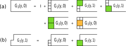
Figure 5: Diagrammatic representation of the recursion relation obeyed by the generating functions (a) $G_{2}(y,0)$ and (b) $G_{2}(y,1)$ for a track of width 4 [see (58) for definition]. Right hand side enumerates the different ways the first column of the track may be occupied by vacancies (open 1$\times$1 square), square (filled 2$\times$2 green square) and defect (filled 2$\times$2 yellow square).

Consider the following generating function.

$$G_{2}(y,\Delta)=\sum_{\ell=0}^{\infty}\Omega_{2}(\ell,\Delta)y^{2\ell+\Delta},$$ (58)

where the power of $\sqrt{y}$ is the number of sites in the system. $G_{2}(y,0)$ and $G_{2}(y,1)$ obey simple recursion relations which are shown diagrammatically in figure 5. In equation form, they are

$$G_{2}(y,0)= 1+y^{2}G_{2}(y,0)+2zy^{3}G_{2}(y,1)+(z^{2}y^{4}+z_{D}y^{4})G_{2}(y,0),$$ (59)

$$G_{2}(y,1)= yG_{2}(y,0)+zy^{2}G_{2}(y,1),$$ (60)

where $z_{D}$ is the activity associated with each defect square. These relations are easily solved to give

$$G_{2}(y,0) = \frac{1-zy^{2}}{f(y^{2})},$$ (61)

$$G_{2}(y,1) = \frac{y}{f(y^{2})},$$ (62)

where

$$f(y)=z(z^{2}+z_{D})y^{3}-(z^{2}+z+z_{D})y^{2}-(1+z)y+1.$$

Let $y_{2}$ be the smallest root of $f(y)=0$. For very large $\ell$, we may write $\Omega_{2}(\ell,\Delta)$ as

$$\Omega_{2}(\ell,\Delta)=a_{2}(\Delta)\lambda_{2}^{2\ell+\Delta}[1+O(\exp(-c\ell))],~{}\ell\gg 1,~{}c>0,$$ (63)

where

$$\lambda_{2}=\frac{1}{\sqrt{y_{2}}}.$$ (64)

Calculating coefficient of $y^{2\ell+\Delta}$, the prefactor $a_{2}(\Delta)$ for $\Delta=0,1$ is obtained to be

$$a_{2}(0) = \frac{-(1-zy_{2})}{y_{2}f^{\prime}(y_{2})},$$ (65)

$$a_{2}(1) = \frac{-1}{\sqrt{y_{2}}f^{\prime}(y_{2})}.$$ (66)

We now consider $\Delta\geq 2$. The recursion relation obeyed by $\Omega_{2}(\ell,\Delta)$ for $\Delta\geq 2$ is shown diagrammatically in figure 6, and may be written mathematically as

$$\Omega_{2}(\ell,\Delta)=\Omega_{2}(\ell,\Delta-1)+z\Omega_{2}(\ell,\Delta-2),~{}~{}\Delta=2,3,...$$ (67)

We define the generating function

$$F(\ell,x)=\sum_{\Delta=0}^{\infty}\Omega_{2}(\ell,\Delta)x^{\Delta}.$$ (68)

Multiplying (67) by $x^{\Delta}$ and summing from $2$ to $\infty$, we obtain a linear equation obeyed by $F(\ell,x)$ which is easily solved to give

$$F(\ell,x)=\frac{\Omega_{2}(\ell,0)+x\big{[}\Omega_{2}(\ell,1)-\Omega_{2}(\ell,0)\big{]}}{1-x-zx^{2}},$$ (69)

where $\Omega_{2}(\ell,0)$ and $\Omega_{2}(\ell,1)$ have already been determined [see (61), (62)]. $F(\ell,x)$ has two simple poles at

$$x_{\pm}=\frac{-1\pm\sqrt{1+4z}}{2z}.$$ (70)

Expanding the denominator about its two roots $x_{\pm}$, we determine $\Omega_{2}(\ell,\Delta)$ by calculating the coefficient of $x^{\Delta}$. We obtain

$$a_{2}(\Delta)=A_{+}(x_{+}\lambda_{2})^{-\Delta}+A_{-}(x_{-}\lambda_{2})^{-\Delta},~{}\Delta=0,1,2...,$$ (71)

where

$$A_{\pm}=\frac{\pm\big{[}\lambda_{2}a_{2}(1)-(zx_{\mp}+1)a_{2}(0)\big{]}}{\sqrt{1+4z}}.$$ (72)

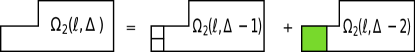
Figure 6: Diagrammatic representation of the recursion relation obeyed by the partition function $\Omega_{2}(\ell,\Delta)$ with $\Delta\geq 2$, for a track of width 4. The first column of the track may be occupied by two vacancies (open 1$\times$1 square) or a square (filled 2$\times$2 square).

4.3 Calculation of $a_{2}^{(L)}(\Delta)$

In this section, we calculate the pre-factor $a_{2}^{(L)}(\Delta)$ that characterizes the asymptotic behavior of the partition function of track of width 4 [see (12)] for the left phase. The left phase has the constraint that the right edge of the rightmost square must touch the interface [see discussion in the paragraph following (6)]. Thus

$$\Omega_{2}^{(L)}(\ell,\Delta)=z^{2}\Omega_{2}(\ell-2,\Delta),$$ (73)

where the factor $z^{2}$ accounts for the two squares adjacent to interface. Once these two squares are placed the occupation of the rest of the track has no constraints and hence enumerated by $\Omega_{2}(\ell-2,\Delta)$. Using (73), (12) and (63), for very large $\ell$ we obtain

$$a_{2}^{(L)}(\Delta)=\frac{z^{2}}{\lambda_{2}^{4}}a_{2}(\Delta),$$ (74)

where $a_{2}(\Delta)$ is given in (71).

4.4 Calculation for $a_{2}^{(R)}(\Delta)$

In this section, we calculate $a_{2}^{(R)}(\Delta)$ for $\Delta\geq 0$, as defined in (13). Consider the track labeled by $(\xi_{i},\xi_{i+1})$ [see figure 2]. The constraint on the right phase is that a defect is allowed to be present only to to the right of $\min(\xi_{i},\xi_{i+1})$ and there must be at least one non-defect square present to its left [see discussion in the paragraph following (6)]..

First consider $\Delta=0,1$. The recursion relation obeyed by the partition functions $\Omega_{2}^{(R)}(\ell,0)$ and $\Omega_{2}^{(R)}(\ell,1)$ for right phase are shown diagrammatically in figure 7 and may be written as

$$\Omega_{2}^{(R)}(\ell,0) = \Omega_{2}^{(R)}(\ell-1,0)+2z\Omega_{2}(\ell-2,1)+z^{2}\Omega_{2}(\ell-2,0),$$ (75)

$$\Omega_{2}^{(R)}(\ell,1) = \Omega_{2}^{(R)}(\ell,0)+z\Omega_{2}(\ell-1,1).$$ (76)

Using the asymptotic expressions for the partition functions as given in (11) and (13), we obtain two linear equations for $a_{2}^{(R)}(0)$ and $a_{2}^{(R)}(1)$, which are easily solved to give

$$a_{2}^{(R)}(0) = \frac{z\big{[}2a_{2}(1)\lambda_{2}+za_{2}(0)\big{]}}{\lambda_{2}^{2}(\lambda_{2}^{2}-1)},$$ (77)

$$a_{2}^{(R)}(1) = \frac{\lambda_{2}a_{2}^{(R)}(0)+za_{2}(1)}{\lambda_{2}^{2}}.$$ (78)

Figure 7: Diagrammatic representation of the recursion relation obeyed by the partition functions $\Omega_{2}^{(R)}(\ell,0)$ and $\Omega_{2}^{(R)}(\ell,1)$ for the track of width 4. Right hand side enumerates the different ways the first column of the track may be occupied by vacancies (open 1$\times$1 square) or squares (filled 2$\times$2 square).

Now consider $\Delta\geq 2$. The recursion relation obeyed by $\Omega_{2}^{(R)}(\ell,\Delta)$ for $\Delta\geq 2$ may be written as

$$\Omega_{2}^{(R)}(\ell,\Delta)=\Omega_{2}^{(R)}(\ell,\Delta-1)+z\widetilde{\Omega}_{2}(\ell,\Delta-2)$$ (79)

where $\widetilde{\Omega}_{2}(\ell,\Delta)$ is the partition function for a generalization of the shape for $\Omega_{2}^{(R)}(\ell,1)$ in the left hand side of figure 7. The lack of the subscript $(R)$ means that there are no constraints. The first term in the right hand side of (79) corresponds to placing vacancies in first column, and the second term to a non-defect square being placed. $\Omega_{2}^{(R)}(\ell,\Delta-1)$ in the right hand side of (79) may be iterated further to yield

$$\Omega_{2}^{(R)}(\ell,\Delta)=\Omega_{2}^{(R)}(\ell,1)+z\sum_{i=0}^{\Delta-2}\widetilde{\Omega}_{2}(\ell,i),$$ (80)

To solve (80), consider the generating function $\widetilde{G}_{2}(y,\Delta)$ defined as

$$\widetilde{G}_{2}(y,\Delta)=\sum_{\ell=0}^{\infty}\widetilde{\Omega}_{2}(\ell,\Delta)y^{2\ell+3\Delta/2},$$ (81)

where power of $\sqrt{y}$ gives total number of sites in the system. The diagrammatic representation of the recursion relation obeyed by $\widetilde{G}_{2}(y,1)$ is shown in figure 8 and may be written as

$$\widetilde{G}_{2}(y,1)=y^{3/2}{G}_{2}(y,0)+zy^{5/2}G_{2}(y,1)+z_{D}y^{7/2}G_{2}(y,0),$$ (82)

where $z_{D}$ is the activity associated with each defect, and $G_{2}(y,0)$ and $G_{2}(y,1)$ are as in (61) and (62). The generating function $\widetilde{G}_{2}(y,1)$ is then easily solved to give

$$\widetilde{G}_{2}(y,1)=\frac{(1+z_{D}y^{2}-zz_{D}y^{4})y^{3/2}}{f(y^{2})}.$$ (83)

For large $\ell$ the partition function may be written asymptotically as

$$\widetilde{\Omega}_{2}(\ell,\Delta)=\widetilde{a}_{2}(\Delta)\lambda_{2}^{2\ell+\Delta},~{}\Delta\geq 0,~{}\ell\gg 1.$$ (84)

Calculating the coefficient of $y^{2\ell+3/2}$ from (83) and using (84), we obtain the prefactor

$$\widetilde{a}_{2}(1)=\frac{-(1+z_{D}y_{2}-zz_{D}y_{2}^{2})}{\sqrt{y_{2}}f^{\prime}(y_{2})}.$$ (85)

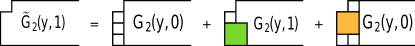
Figure 8: Diagrammatic representation of the recursion relation obeyed by the generating function $\widetilde{G}_{2}(y,1)$ [see (81) for definition] for a track of width 4. Right hand side enumerates the different ways the first column of the track may be occupied by vacancies (open 1$\times$1 square), square (filled 2$\times$2 square of color green) and defect (filled 2$\times$2 square of color yellow).

Now calculate the partition function $\widetilde{\Omega}_{2}(\ell,\Delta)$ for $\Delta\geq 2$. The diagrammatic representation of the recursion relation obeyed by the partition function $\widetilde{\Omega}_{2}(\ell,\Delta)$ for $\Delta\geq 2$ is shown in figure 9 and may be written mathematically as

$$\widetilde{\Omega}_{2}(\ell,\Delta)=\widetilde{\Omega}_{2}(\ell,\Delta-1)+(z+z_{D})\widetilde{\Omega}_{2}(\ell,\Delta-2),~{}\Delta=2,3,....$$ (86)

We define the generating function

$$H(\ell,t)=\sum_{\Delta=0}^{\infty}\widetilde{\Omega}_{2}(\ell,\Delta)t^{\Delta}.$$ (87)

Multiplying (86) by $t^{\Delta}$ and performing summation over $\Delta$ from $2$ to $\infty$, we obtain a linear equation obeyed by $H(\ell,t)$ which is solved to give

$$H(\ell,t)=\frac{\widetilde{\Omega}_{2}(\ell,0)+t\left[\widetilde{\Omega}_{2}(\ell,1)-\widetilde{\Omega}_{2}(\ell,0)\right]}{1-t-(z+z_{D})t^{2}}.$$ (88)

$H(\ell,t)$ has two simple poles determined by the roots of the quadratic equation $1-t-(z+z_{D})t^{2}=0$

$$t_{\pm}=\frac{-1\pm\sqrt{1+4(z+z_{D})}}{2(z+z_{D})}.$$ (89)

Expanding the denominator about $t_{\pm}$ and calculating the coefficient of $t^{\Delta}$, we get the expression for $\widetilde{\Omega}_{2}(\ell,\Delta)$ and using (84) the prefactor is obtained to be

$$\widetilde{a}_{2}(\Delta)=B_{+}(t_{+}\lambda_{2})^{-\Delta}+B_{-}(t_{-}\lambda_{2})^{-\Delta},~{}\Delta\geq 0,$$ (90)

where

$$B_{\pm}=\frac{\pm\bigg{[}\lambda_{2}\widetilde{a}_{2}(1)-[(z+z_{D})t_{\mp}+1]a_{2}(0)\bigg{]}}{\sqrt{1+4(z+z_{D})}}.$$ (91)

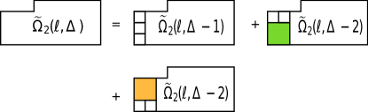
Figure 9: Diagrammatic representation of the recursion relation obeyed by the partition function $\widetilde{\Omega}_{2}(\ell,\Delta)$ with $\Delta\geq 2$ for a track of width 4. Right hand side enumerates the different ways the first column of the track may be occupied by vacancies (open 1$\times$1 square), square (filled 2$\times$2 square of color green) and defect (filled 2$\times$2 square of color yellow).

We now return to (80) and replace the partition functions $\Omega_{2}^{(R)}(\ell,\Delta)$ and $\widetilde{\Omega}_{2}(\ell,i)$ by their asymptotic forms given in (13) and (84) respectively, and do the summation over $\widetilde{\Omega}_{2}(\ell,i)$ from $i=0$ to $(\Delta-2)$, to obtain the prefactor

$$a_{2}^{(R)}(\Delta)=v_{1}\lambda_{2}^{-\Delta}+v_{2}(t_{+}\lambda_{2})^{-\Delta}+v_{3}(t_{-}\lambda_{2})^{-\Delta},~{}\Delta\geq 2,$$ (92)

where

$$v_{1} = a_{2}^{(R)}(1)\lambda_{2}+z\bigg{(}\frac{B_{+}t_{+}}{t_{+}-1}+\frac{B_{-}t_{-}}{t_{-}-1}\bigg{)},$$

$$v_{2} = -\frac{zB_{+}t_{+}^{2}}{t_{+}-1},$$

$$v_{3} = -\frac{zB_{-}t_{-}^{2}}{t_{-}-1}.$$

5 Results

In this section we determine the interfacial tension $\sigma(z)$ between two ordered phases as a function of the activity $z$. From (28), $\sigma(z)$ may be written as

$$\sigma(z)=-\frac{1}{2}\log\bigg{[}\frac{\lambda_{1}^{2}\Lambda_{2}}{za_{1}a_{2}(0)}\bigg{]},$$ (93)

where $\Lambda_{2}$, $\lambda_{1}$, $a_{1}$ and $a_{2}(0)$ are as in (51), (57), and (65). $\Lambda_{2}$ depends on $a_{2}^{(L)}(\Delta)$ and $a_{2}^{(R)}(\Delta)$, which in turn have been calculated in (74) and (92). We also set $z_{D}=z$, where $z_{D}$ is the activity of a defect.

The variation of $\sigma(z)$ with activity $z$ is shown in figure 10. It decreases monotonically with decreasing $z$ and becomes zero at a finite value of $z$, which will be our estimate of the critical activity $z_{c}$. We find that $z_{c}=105.35$ for the interface with overhangs. As a check for the calculation, we confirm that if we set $z_{D}=0$, then we obtain the results for the estimated $z_{c}$ in the absence of defects [18]. The result for $z_{c}$ compares well with the numerical estimate from Monte Carlo simulations of $z_{c}\approx 97.5$ [see table 1].

Figure 10: The variation of the interfacial tension $\sigma(z)$ with activity $z$. Interfacial tension $\sigma(z)$ vanishes at the critical activity $z=z_{c}$.

The occupied area fraction or density $\rho$ may be calculated from the partition function $Z^{(0)}$ as:

$$\rho=\frac{4z}{N_{x}N_{y}}\frac{\partial}{\partial z}\bigg{[}\log\big{(}Z^{(0)}\big{)}\bigg{]},$$ (94)

where the factor $4$ accounts for the area of a square. Substituting for $Z^{(0)}$ from (22), the density $\rho$ in (94), in the thermodynamic limit $N_{x}\rightarrow\infty,~{}N_{y}\rightarrow\infty$, reduces to

$$\rho=4z\bigg{[}\frac{1}{\lambda_{2}}\frac{\partial\lambda_{2}}{\partial z}-\frac{1}{2\lambda_{1}}\frac{\partial\lambda_{1}}{\partial z}\bigg{]}.$$ (95)

We thus obtain the critical density to be $\rho_{c}=0.947$. This estimate compare well with the Monte Carlo results of $\rho_{c}\approx 0.932$ [see table 1].

6 Conclusion

In this paper, we estimated the transition point of the disordered-columnar transition in in the hard square model by calculating the interfacial tension between two ordered phases within a pairwise approximation. This calculation allows for multiple defects to be present as well as the interface to have effective overhangs. We obtain the critical activity $z_{c}=105.35$ and critical density $\rho_{c}=0.947$, which agrees reasonably with the numerically obtained results of $z_{c}\approx 97.5$ and $\rho_{c}\approx 0.932$. Our estimate for the critical activity is a considerable improvement over earlier estimates based on many different approaches [see table 1].

We calculated the prefactor $a_{2}^{(R)}(\Delta)$ by allowing defects to be present as overhangs [see section 4.4]. The calculation can be repeated when defects are present only in regions which do not correspond to overhangs. This corresponds to a defect in the right phase being present only to the right of $\max(\xi_{i},\xi_{i+1})$ [see figure 2]. This calculation leads to an estimate of $z_{c}=43.28$, which is about half the value of the numerical result of $z_{c}\approx 97.5$. The decrease in the value of $z_{c}$ on excluding overhangs is consistent with the fact that the entropy of the system with interface decreases while the entropy of the system without interface remains unchanged. We, thus, conclude that the presence of overhangs in the interface is important for the calculation of interfacial tension.

A similar analysis for determining the phase boundary may be done for other kind of systems, which show a transition from disordered to columnar ordered phase with increasing density. The mixture of hard squares and dimers [9] shows such a transition, and so does the system of $(d\times 2)$ hard rectangles [29, 30, 18]. It would be interesting to see whether the approximation scheme used in this paper is useful in obtaining reliable estimates for the phase boundaries in these problems.

References

References

- [1] Domb C 1958 Nuovo Cimento 9 9–26
- [2] Bellemans A and Nigam R K 1967 J. Chem. Phys. 46 2922–2935
- [3] Hoover W G and Rocco A G D 1962 J. Chem. Phys. 36 3141–3162
- [4] Kinzel W and Schick M 1981 Phys. Rev. B 24(1) 324–328
- [5] Amar J, Kaski K and Gunton J D 1984 Phys. Rev. B 29 1462–1464
- [6] Ree F H and Chesnut D A 1967 Phys. Rev. Lett. 18(1) 5–8
- [7] Nisbet R and Farquhar I 1974 Physica 76 283 – 294
- [8] Fernandes H C M, Arenzon J J and Levin Y 2007 J. Chem. Phys. 126 114508
- [9] Ramola K, Damle K and Dhar D 2015 Phys. Rev. Lett. 114(19) 190601
- [10] Feng X, Blöte H W J and Nienhuis B 2011 Phys. Rev. E 83(6) 061153
- [11] Zhitomirsky M E and Tsunetsugu H 2007 Phys. Rev. B 75(22) 224416
- [12] Baxter R J 1980 J. Phys. A 13 L61
- [13] Bellemans A and Nigam R K 1966 Phys. Rev. Lett. 16(23) 1038–1039
- [14] Ramola K and Dhar D 2012 Phys. Rev. E 86(3) 031135
- [15] Lafuente L and Cuesta J A 2003 J. Chem. Phys. 119 10832–10843
- [16] Lafuente L and Cuesta J A 2002 J. Phys. Condens. Matter 14 12079
- [17] Slotte P A 1983 J. Phys. C 16 2935
- [18] Nath T, Dhar D and Rajesh R 2016 Europhys. Lett. 114 10003
- [19] Marques Fernandes H C, Levin Y and Arenzon J J 2007 Phys. Rev. E 75(5) 052101
- [20] Temperley H N V 1961 Proc. Phys. Soc. 77 630
- [21] de Gennes P and Prost J 1995 The physics of liquid crystals (International series of monographs on physics vol 23) (Oxford University Press)
- [22] Bak P, Kleban P, Unertl W N, Ochab J, Akinci G, Bartelt N C and Einstein T L 1985 Phys. Rev. Lett. 54(14) 1539–1542
- [23] Taylor D E, Williams E D, Park R L, Bartelt N C and Einstein T L 1985 Phys. Rev. B 32(7) 4653–4659
- [24] Mitchell S, Brown G and Rikvold P 2001 Surf. Sci. 471 125 – 142
- [25] Zhang Y, Blum V and Reuter K 2007 Phys. Rev. B 75(23) 235406
- [26] Koper M T 1998 J. Electroanal. Chem. 450 189 – 201
- [27] Kundu J and Rajesh R 2014 Phys. Rev. E 89(5) 052124
- [28] Kundu J and Rajesh R 2015 Euro. Phys. J. B 88 133
- [29] Kundu J and Rajesh R 2015 Phys. Rev. E 91(1) 012105
- [30] Nath T, Kundu J and Rajesh R 2015 J. Stat. Phys. 160 1173–1197
- [31] Alet F, Ikhlef Y, Jacobsen J L, Misguich G and Pasquier V 2006 Phys. Rev. E 74(4) 041124
- [32] Nath T and Rajesh R 2014 Phys. Rev. E 90(1) 012120
- [33] Nath T and Rajesh R 2016 J. Stat. Mech. 2016 073203
- [34] Papanikolaou S, Luijten E and Fradkin E 2007 Phys. Rev. B 76(13) 134514
- [35] Ralko A, Poilblanc D and Moessner R 2008 Phys. Rev. Lett. 100(3) 037201
- [36] Wenzel S, Coletta T, Korshunov S E and Mila F 2012 Phys. Rev. Lett. 109(18) 187202
- [37] Jin S and Sandvik A W 2013 Phys. Rev. B 87(18) 180404
- [38] Baxter R J 1999 Ann. Comb. 3 191–203
- [39] Blair D W, Santangelo C and Machta J 2012 J. Stat. Mech. 2012 P01018
- [40] Decaudin P and Neyret F 2004 Eurographics 49–52
- [41] Zhao K, Bruinsma R and Mason T G 2011 Proc. Natl. Acad. Sci. 108 2684–2687
- [42] Walsh L and Menon N 2016 J. Stat. Mech. 2016 083302
- [43] Kundu J, Rajesh R, Dhar D and Stilck J F 2012 AIP Conf. Proc. 1447 113–114
- [44] Kundu J, Rajesh R, Dhar D and Stilck J F 2013 Phys. Rev. E 87(3) 032103