Refined open intersection numbers and the Kontsevich-Penner matrix model

Abstract.

A study of the intersection theory on the moduli space of Riemann surfaces with boundary was recently initiated in a work of R. Pandharipande, J. P. Solomon and the third author, where they introduced open intersection numbers in genus $0$. Their construction was later generalized to all genera by J. P. Solomon and the third author. In this paper we consider a refinement of the open intersection numbers by distinguishing contributions from surfaces with different numbers of boundary components, and we calculate all these numbers. We then construct a matrix model for the generating series of the refined open intersection numbers and conjecture that it is equivalent to the Kontsevich-Penner matrix model. An evidence for the conjecture is presented. Another refinement of the open intersection numbers, which describes the distribution of the boundary marked points on the boundary components, is also discussed.

1. Introduction

A compact Riemann surface is a compact connected complex manifold of dimension $1$. Denote by $\mathcal{M}_{g,l}$ the moduli space of all compact Riemann surfaces of genus $g$ with $l$ marked points. P. Deligne and D. Mumford defined a natural compactification $\mathcal{M}_{g,l}\subset\overline{\mathcal{M}}_{g,l}$ via stable curves (with possible nodal singularities) in [DM69]. The moduli space $\overline{\mathcal{M}}_{g,l}$ is a non-singular complex orbifold of dimension $3g-3+l$. It is defined to be empty unless the stability condition

(1.1) $$2g-2+l>0$$

is satisfied. We refer the reader to [DM69, HM98] for the basic theory.

In his seminal paper [Wit91], E. Witten initiated new directions in the study of $\overline{\mathcal{M}}_{g,l}$. For each marking index $i$ consider the cotangent line bundle $\mathbb{L}_{i}\rightarrow\overline{\mathcal{M}}_{g,l}$, whose fiber over a point $[\Sigma,z_{1},\ldots,z_{l}]\in\overline{\mathcal{M}}_{g,l}$ is the complex cotangent space $T_{z_{i}}^{*}\Sigma$ of $\Sigma$ at $z_{i}$. Let $\psi_{i}\in H^{2}(\overline{\mathcal{M}}_{g,l},\mathbb{Q})$ denote the first Chern class of $\mathbb{L}_{i}$, and write

(1.2) $$\left<\tau_{a_{1}}\tau_{a_{2}}\cdots\tau_{a_{l}}\right>_{g}^{c}:=\int_{\overline{\mathcal{M}}_{g,l}}\psi_{1}^{a_{1}}\psi_{2}^{a_{2}}\cdots\psi_{l}^{a_{l}}.$$

The integral on the right-hand side of (1.2) is well-defined, when the stability condition (1.1) is satisfied, all the $a_{i}$ are non-negative integers and the dimension constraint $3g-3+l=\sum a_{i}$ holds. In all other cases $\left<\prod\tau_{a_{i}}\right>_{g}^{c}$ is defined to be zero. The intersection products (1.2) are often called descendent integrals or intersection numbers. Let $t_{i}$, $i\geq 0$, be formal variables and let

$$F^{c}(t_{0},t_{2},\ldots):=\sum_{g\geq 0}F_{g}^{c}(t_{0},t_{1},\ldots),\quad\text{where}$$

$$F^{c}_{g}(t_{0},t_{1},\ldots):=\sum_{l\geq 1}\sum_{a_{1},\ldots,a_{l}\geq 0}\left<\tau_{a_{1}}\tau_{a_{2}}\cdots\tau_{a_{l}}\right>^{c}_{g}\frac{\prod t_{a_{i}}}{l!}.$$

The generating series $F^{c}$ is called the closed free energy. The exponent $\tau^{c}:=\exp(F^{c})$ is called the closed partition function. Witten’s conjecture ([Wit91]), proved by M. Kontsevich ([Kon92]), says that the closed partition function $\tau^{c}$ becomes a tau-function of the KdV hierarchy after the change of variables $t_{n}=(2n+1)!!T_{2n+1}$. Integrability immediately follows [KMMMZ92] from Kontsevich’s matrix integral representation

(1.3) $$\left.\tau^{c}\right|_{T_{k}=\frac{1}{k}\mathop{\mathrm{tr}}\nolimits\Lambda^{-k}}=c_{\Lambda,M}\int_{\mathcal{H}_{M}}e^{\frac{1}{6}\mathop{\mathrm{tr}}\nolimits H^{3}-\frac{1}{2}\mathop{\mathrm{tr}}\nolimits H^{2}\Lambda}dH,$$

where one integrates over the space of Hermitian $M\times M$ matrices, $\Lambda=\mathop{\mathrm{diag}}\nolimits(\lambda_{1},\ldots,\lambda_{M})$ is a diagonal matrix with positive real entries and

$$c_{\Lambda,M}:=(2\pi)^{-\frac{M^{2}}{2}}\prod_{i=1}^{M}\sqrt{\lambda_{i}}\prod_{1\leq i<j\leq M}(\lambda_{i}+\lambda_{j}).$$

In [PST14] the authors started to develop a parallel theory for Riemann surfaces with boundary. A Riemann surface with boundary is a connected $1$ dimensional complex manifold with finite positive number of circular boundaries, each with a holomorphic collar structure. A compact Riemann surface is not viewed here as a Riemann surface with boundary. Given a Riemann surface with boundary $(X,\partial X)$, we can canonically construct a double via Schwarz reflection through the boundary. The double $D(X,\partial X)$ of $(X,\partial X)$ is a compact Riemann surface. The doubled genus of $(X,\partial X)$ is defined to be the usual genus of $D(X,\partial X)$. On a Riemann surface with boundary $(X,\partial X)$, we consider two types of marked points. The markings of interior type are points of $X\backslash\partial X$. The markings of boundary type are points of $\partial X$. Let $\mathcal{M}_{g,k,l}^{\mathbb{R}}$ denote the moduli space of Riemann surfaces with boundary of doubled genus $g$ with $k$ distinct boundary markings and $l$ distinct interior markings. The moduli space $\mathcal{M}_{g,k,l}^{\mathbb{R}}$ is defined to be empty unless the stability condition

$$2g-2+k+2l>0$$

is satisfied. The moduli space $\mathcal{M}_{g,k,l}^{\mathbb{R}}$ may have several connected components depending upon the topology of $(X,\partial X)$ and the cyclic orderings of the boundary markings. Foundational issues concerning the construction of $\mathcal{M}_{g,k,l}^{\mathbb{R}}$ are addressed in [Liu02]. The moduli space $\mathcal{M}_{g,k,l}^{\mathbb{R}}$ is a real orbifold of real dimension $3g-3+k+2l$, it is in general not compact and may be not orientable when $g>0.$

Since interior marked points have well-defined cotangent spaces, there is no difficulty in defining the cotangent line bundles $\mathbb{L}_{i}\to\mathcal{M}_{g,k,l}^{\mathbb{R}}$ for each interior marking, $i=1,\ldots,l$. Naively, one may want to consider a descendent theory via integration of products of the first Chern classes $\psi_{i}=c_{1}(\mathbb{L}_{i})\in H^{2}(\overline{\mathcal{M}}_{g,k,l}^{\mathbb{R}},\mathbb{Q})$ over a compactification $\overline{\mathcal{M}}_{g,k,l}^{\mathbb{R}}$ of $\mathcal{M}_{g,k,l}^{\mathbb{R}}$. Namely,

(1.4) $$\left<\tau_{a_{1}}\tau_{a_{2}}\cdots\tau_{a_{l}}\sigma^{k}\right>^{o}_{g}:=2^{-\frac{g+k-1}{2}}\int_{\overline{\mathcal{M}}_{g,k,l}^{\mathbb{R}}}\psi_{1}^{a_{1}}\psi_{2}^{a_{2}}\cdots\psi_{l}^{a_{l}},$$

when

$$2\sum a_{i}=3g-3+k+2l,$$

and in all other cases $\left<\tau_{a_{1}}\tau_{a_{2}}\cdots\tau_{a_{l}}\sigma^{k}\right>^{o}_{g}:=0$. Note that, in particular, $g+k$ must always be odd in order to get non-zero numbers. The new insertion $\sigma$ corresponds to the addition of a boundary marking. The coefficient in front of the integral on the right-hand side of (1.4) appears to be useful for the description of the new intersection numbers, that are called the open intersection numbers, in terms of integrable systems.

In genus $0$ the moduli $\overline{\mathcal{M}}_{0,k,l}:=\overline{\mathcal{M}}_{0,k,l}^{\mathbb{R}}$ is canonically oriented for $k$ odd, and one can calculate an integral of the form $\int_{\overline{\mathcal{M}}_{0,k,l}}\psi_{1}^{a_{1}}\psi_{2}^{a_{2}}\cdots\psi_{l}^{a_{l}},$ given boundary conditions for the line bundles $\mathbb{L}_{i}.$ More precisely, given nowhere vanishing boundary conditions $s\in C^{\infty}(E\to\partial\overline{\mathcal{M}}_{0,k,l}),$ for $E=\bigoplus\mathbb{L}_{i}^{\oplus a_{i}},$ one may define the integral (1.4) by

(1.5) $$\left<\tau_{a_{1}}\tau_{a_{2}}\cdots\tau_{a_{l}}\sigma^{k}\right>^{o}_{0}:=2^{-\frac{k-1}{2}}\int_{\overline{\mathcal{M}}_{0,k,l}}e(E,s),$$

where $e(E,s)$ is the relative Euler class. The result depends on the boundary conditions.

In [PST14] a family of boundary conditions, called canonical boundary conditions for each bundle $\mathbb{L}_{i}$ is constructed. It is proven that for a generic choice of canonical boundary conditions, $s_{ij}\in C^{\infty}_{m}(\mathbb{L}_{i}\to\partial\overline{\mathcal{M}}_{0,k,l}),~{}i\in[l],j\in[a_{i}]$, the boundary conditions $s=\bigoplus s_{ij}$ is nowhere vanishing along $\partial\overline{\mathcal{M}}_{0,k,l},$ assuming $2\sum a_{i}=3g-3+k+2l$. Here we use the notation $[l]$ for a set $\{1,2,\ldots,l\}$ and the subscript $m$ indicates that multi-valued section, rather than sections, are used. It is then shown that any two generic choices of canonical boundary conditions give rise to the same integral (1.5). In [PST14] all open intersection numbers for doubled genus $0$ were calculated, and the authors proposed a conjectural description of the open intersection numbers in all genera. Let $s$ be a formal variable. Define

$$F^{o}(t_{0},t_{1},\ldots,s):=\sum_{g\geq 0}F^{o}_{g}(t_{0},t_{1},\ldots,s),\quad\text{where}$$

$$F^{o}_{g}(t_{0},t_{1},\ldots,s):=\sum_{k,l\geq 0}\sum_{a_{1},\ldots,a_{l}\geq 0}\left<\tau_{a_{1}}\cdots\tau_{a_{l}}\sigma^{k}\right>^{o}_{g}\frac{s^{k}\prod t_{a_{i}}}{k!l!}.$$

The generating series $F^{o}$ is called the open free energy and the exponent $\tau^{o}:=\exp(F^{o}+F^{c})$ is called the open partition function. The conjecture of R. Pandharipande, J. P. Solomon and the third author ([PST14]) says that the generating series $F^{o}$ satisfies a certain system of partial differential equations that is called in [PST14] the open KdV equations.

In higher genus the construction of open intersection numbers needs some refinement. Firstly, the moduli space $\mathcal{M}_{g,k,l}$ is in general non-orientable for $g>0.$ In order to overcome this issue, J. P. Solomon and the third author define graded spin surfaces, which are open surfaces with a spin structure and some extra structure. In [STa] the moduli of graded spin surfaces $\overline{\mathcal{M}}_{g,k,l}$ is defined and is proved to be canonically oriented. When $g=0$ it coincides with $\overline{\mathcal{M}}_{0,k,l}^{\mathbb{R}}.$ Canonical boundary conditions are then constructed for the line bundles $\mathbb{L}_{i},$ and again it is proven that one can define

(1.6) $$\left<\tau_{a_{1}}\tau_{a_{2}}\cdots\tau_{a_{l}}\sigma^{k}\right>^{o}_{g}:=2^{-\frac{g+k-1}{2}}\int_{\overline{\mathcal{M}}_{g,k,l}}e(E,s),$$

where $e(E,s)$ is the relative Euler with respect to the canonical boundary conditions. As in $g=0,$ generic choices of canonical boundary conditions give rise to the same integrals. It should be stressed that, although [STa] has not appeared yet, the moduli and boundary conditions mentioned above are fully described in Section 2 of [Tes15].

A combinatorial formula for the open intersection numbers was found in [Tes15]. The conjecture of R. Pandharipande, J. P. Solomon and the third author was proved in [BT15]. Properties of the open free energy $F^{o}$ were intensively studied in [Ale15a, Ale15b, Ale16, Bur15, Bur16, Saf16a]. In particular, in [Bur15, Bur16] the second author introduced a formal power series $F^{o,ext}(t_{0},t_{1},\ldots,s_{0},s_{1},\ldots)$, where $s_{0}=s$ and $s_{1},s_{2},\ldots$ are new formal variables. The function $F^{o,ext}$ is an extension of the open free energy $F^{o}$,

$$\left.F^{o,ext}\right|_{s_{\geq 1}=0}=F^{o},$$

and, therefore, it was called the extended open free energy. The exponent $\tau^{o,ext}:=\exp(F^{o,ext}+F^{c})$ was called the extended open partition function. In [Bur15, Bur16] the new variables $s_{i}$, $i\geq 1$, appeared naturally from the point of view of integrable systems. The second author suggested to consider them as descendents of the boundary marked points. A geometric construction of the descendent theory for the boundary marked points, a derivation of the combinatorial formula for it, and a geometric proof of the conjecture of [Bur15] regarding the extended theory, will appear in [STb],[Tes].

In [Bur16] the second author found a simple relation of the extended open partition function $\tau^{o,ext}$ to the wave function of the Kontsevich-Witten tau-function. In [Ale15b] the first author proved that both extended open partition function and closed partition function belong to the same family of tau-functions, described by the matrix integrals of Kontsevich type. Namely, the Kontsevich-Penner integral

(1.7) $$\left.\tau_{N}\right|_{T_{k}=\frac{1}{k}\mathop{\mathrm{tr}}\nolimits\Lambda^{-k}}:=c_{\Lambda,M}\int_{\mathcal{H}_{M}}e^{\frac{1}{6}\mathop{\mathrm{tr}}\nolimits H^{3}-\frac{1}{2}\mathop{\mathrm{tr}}\nolimits H^{2}\Lambda}\frac{\det^{N}\Lambda}{\det^{N}(\Lambda-H)}dH$$

for $N=0$ coincides with Kontsevich’s integral (1.3). In [Ale15b] it was shown that for $N=1$ it describes the extended open partition function. From this matrix integral representation it immediately follows that the extended open partition function is a tau-function of the KP hierarchy, moreover, it is related to the closed partition function $\tau^{c}$ by equations of the modified KP hierarchy [KMMM93]. A full set of the Virasoro and W-constrains for the tau-function, described by the Kontsevich-Penner matrix integral (1.7), was derived in [Ale15b] for arbitrary $N$. Later these constraints were described by the first author [Ale16] in terms of the so-called free bosonic fields.

1.1. Refined, very refined and extended refined open intersection numbers

As we already discussed above, the moduli space $\mathcal{M}_{g,k,l}$ may have several components depending upon the topology of Riemann surface with boundary. For $b\geq 1$, denote by $\mathcal{M}_{g,k,l,b}$ the submoduli of $\mathcal{M}_{g,k,l}$ that consists of isomorphism classes of surfaces with boundary with $b$ boundary components. So we have the decomposition

$$\mathcal{M}_{g,k,l}=\bigsqcup_{\begin{subarray}{c}1\leq b\leq g+1\\ b+g=1(\mathrm{mod}\,\,2)\end{subarray}}\mathcal{M}_{g,k,l,b}.$$

We can decompose further. Let $P(k,b)$ be the set of unordered $b$-tuples of non-negative integers $\overline{k}=(k_{1},\ldots,k_{b})$, $k_{i}\geq 0$, such that $\sum k_{i}=k$. For $\overline{k}=(k_{1},\ldots,k_{b})\in P(k,b)$ let $\mathcal{M}_{g,\bar{k},l}\subset\mathcal{M}_{g,k,l,b}$ be the submoduli of graded smooth Riemann surfaces with boundary of genus $g$, with $l$ internal marked points, $b$ boundary components and $k$ boundary marked points distributed on the boundary components according to the $b$-tuple $\overline{k}$. Clearly,

$$\mathcal{M}_{g,k,l,b}=\bigsqcup_{\bar{k}\in P(k,b)}\mathcal{M}_{g,\bar{k},l}.$$

It is also easy to see that if we define $\overline{\mathcal{M}}_{g,k,l,b}$ as the closure of $\mathcal{M}_{g,k,l,b}$ in $\overline{\mathcal{M}}_{g,k,l}$ and $\overline{\mathcal{M}}_{g,\overline{k},l}$ as the closure of $\mathcal{M}_{g,\overline{k},l}$ in $\overline{\mathcal{M}}_{g,k,l,b}$, then

$$\overline{\mathcal{M}}_{g,k,l}= \bigsqcup_{\begin{subarray}{c}1\leq b\leq g+1\\ b+g=1(\mathrm{mod}\,\,2)\end{subarray}}\overline{\mathcal{M}}_{g,k,l,b},$$

$$\overline{\mathcal{M}}_{g,k,l,b}= \bigsqcup_{\bar{k}\in P(k,b)}\overline{\mathcal{M}}_{g,\bar{k},l}.$$

In [STa] the authors defined open intersection numbers over any connected component of the moduli space $\overline{\mathcal{M}}_{g,k,l}$. To be precise, they proved the following result.

Theorem 1.1.

Let $a_{1},\ldots,a_{l},k$ be non-negative integers satisfying $2\sum a_{i}=3g-3+k+2l,$ and let $E=\sum_{i=1}^{k}\mathbb{L}_{i}^{\oplus a_{i}}.$ Then for any connected component $C$ of $\overline{\mathcal{M}}_{g,k,l}$ there exist nowhere vanishing canonical boundary conditions $s$ in the sense of [PST14],[STa]. Thus one may define the integral $\int_{C}e(E,s)$. Moreover, any two nowhere vanishing choices of the canonical boundary conditions give rise to the same integral.

The theorem allows us to define refined open intersection numbers as the integrals of monomials in psi-classes over the components $\overline{\mathcal{M}}_{g,k,l,b}$ of $\overline{\mathcal{M}}_{g,k,l}$ and very refined open intersection numbers as the corresponding integrals over the components $\overline{\mathcal{M}}_{g,\bar{k},l}$:

(1.8) $$\left<\tau_{a_{1}}\tau_{a_{2}}\cdots\tau_{a_{l}}\sigma^{k}\right>^{o}_{g,b}:= 2^{-\frac{g+k-1}{2}}\int_{\overline{\mathcal{M}}_{g,k,l,b}}e(E,s),$$

(1.9) $$\left<\tau_{a_{1}}\tau_{a_{2}}\cdots\tau_{a_{l}}\sigma^{\bar{k}}\right>^{o}_{g}:= 2^{-\frac{g+k-1}{2}}\int_{\overline{\mathcal{M}}_{g,\bar{k},l}}e(E,s),$$

where $a_{1},\ldots,a_{l},k,E$ are as in Theorem 1.1 and $s$ is a nowhere vanishing canonical multisection. These new intersection numbers are rational numbers. Let $N$ be a positive integer. Introduce the refined open free energy $F^{o,N}$ by

$$F^{o,N}(t_{0},t_{1},\ldots,s):=\sum_{\begin{subarray}{c}g,k,l\geq 0\\ b\geq 1\end{subarray}}\sum_{a_{1},\ldots,a_{l}\geq 0}\left<\tau_{a_{1}}\cdots\tau_{a_{l}}\sigma^{k}\right>^{o}_{g,b}\frac{N^{b}s^{k}\prod t_{a_{i}}}{k!l!}.$$

Clearly, $F^{o,1}=F^{o}$. Let $q_{0},q_{1},\ldots$ be formal variables. Introduce the very refined open free energy $\widetilde{F}^{o}$ by

$$\widetilde{F}^{o}(t_{0},t_{1},\ldots,q_{0},q_{1},\ldots):=\sum_{\begin{subarray}{c}g,k,l\geq 0\\ b\geq 1\end{subarray}}\sum_{\begin{subarray}{c}\overline{k}=(k_{1},\ldots,k_{b})\in P(k,b)\\ a_{1},\ldots,a_{l}\geq 0\end{subarray}}\left<\tau_{a_{1}}\cdots\tau_{a_{l}}\sigma^{\overline{k}}\right>^{o}_{g}\frac{\prod t_{a_{i}}\prod q_{k_{j}}}{k!l!}.$$

Of course, the function $F^{o,N}$ can be easily expressed in terms of the function $\widetilde{F}^{o}$:

$$F^{o,N}=\left.\widetilde{F}^{o}\right|_{q_{i}=Ns^{i}}.$$

The reason, why we want to consider the refined open free energy $F^{o,N}$ separately, is that it admits a natural extension, while we do not know whether the very refined open free energy $\widetilde{F}^{o}$ can be extended. The exponents $\tau^{o}_{N}:=\exp(F^{o,N}+F^{c})$ and $\widetilde{\tau}^{o}:=\exp(\widetilde{F}^{o}+F^{c})$ will be called the refined open partition function and the very refined open partition function respectively.

In this paper we generalize the result of the third author from [Tes15] and find a combinatorial formula for the very refined open intersection numbers. We also derive matrix models for the refined and the very refined open partition functions. We then show that the form of our matrix model for the refined open partition function $\tau^{o}_{N}$ suggests a natural way to add the variables $s_{i}$, $i\geq 1$, in it. We denote the extended function by $\tau^{o,ext}_{N}$ and call it the extended refined open partition function. This function satisfies the properties

$$\left.\tau^{o,ext}_{N}\right|_{s_{\geq 1}=0}=\tau^{o}_{N},\qquad\tau^{o,ext}_{1}=\tau^{o,ext}.$$

Therefore, it is natural to view the variables $s_{i}$, $i\geq 1$, in the function $\tau^{o,ext}_{N}$ as descendents of the boundary marked points in the refined open intersection theory. We also prove that the extended refined open partition function $\tau^{o,ext}_{N}$ is related to the very refined open partition function $\widetilde{\tau}^{o}$ by a simple transformation. Moreover, we show that this transformation is invertible, so the collection of functions $\tau^{o,ext}_{N}$, $N\geq 1$, and the function $\widetilde{\tau}^{o}$ are in a certain sense equivalent. Finally, we conjecture that the function $\tau^{o,ext}_{N}$ coincides with the tau-function $\tau_{N}$ given by the Kontsevich-Penner matrix integral (1.7) and present an evidence for the conjecture. In particular, we derive the string and the dilaton equations for the function $\tau^{o,ext}_{N}$ and also prove the conjecture in genus $0$ and $1$.

Remark 1.2.

In [Saf16a] the author conjectured that there exists a refinement of the extended open partition function $\tau^{o,ext}$ that distinguishes contributions from Riemann surfaces with different numbers of boundary components and that coincides with the Kontsevich-Penner tau-function $\tau_{N}$. Since we construct this refinement, our conjecture can be considered as a stronger version of the conjecture of B. Safnuk from [Saf16a].

Remark 1.3.

Another approach to refined open intersection numbers was recently suggested by B. Safnuk in [Saf16b]. His approach is quite different to ours, because, in particular, he does not consider boundary marked points and, moreover, he uses a different compactification of $\mathcal{M}_{g,0,l}$. His intersection numbers are given as integrals of some specific volume forms. B. Safnuk also has a combinatorial formula for his refined open intersection numbers and it directly gives the Kontsevich-Penner matrix model. It would be interesting to obtain a direct relation between the two approaches.

1.2. Organization of the paper

In Section 2 we show that the construction of [STa] admits a refinement that allows to define the products (1.8) and (1.9). We also prove combinatorial formulas for the refined and the very refined open intersection numbers. In Section 3 we construct a matrix model for the very refined open partition function $\widetilde{\tau}^{o}_{N}$. We then show that the specialization of it, giving the refined open partition function, has a natural extension, where new variables can be interpreted as descendents of boundary marked points. We prove that the extended refined open partition function $\tau^{o,ext}_{N}$ is related to the very refined open partition function by a simple transformation. We also prove the string and the dilaton equations for $\tau^{o,ext}_{N}$. In Section 4 we formulate our conjecture about the relation between the function $\tau^{o,ext}_{N}$ and the Kontsevich-Penner tau-function $\tau_{N}$ and present an evidence for it.

1.3. Acknowledgements

We would like to thank Leonid Chekhov and Rahul Pandharipande for useful discussions. The work of A.A. was supported in part by IBS-R003-D1, by the Natural Sciences and Engineering Research Council of Canada (NSERC), by the Fonds de recherche du Québec Nature et technologies (FRQNT) and by RFBR grants 15-01-04217 and 15-52-50041YaF. A. B. was supported by Grant ERC-2012-AdG-320368-MCSK in the group of R. Pandharipande at ETH Zurich and Grant RFFI-16-01-00409. R.T. is supported by Dr. Max Rössler, the Walter Haefner Foundation and the ETH Zürich Foundation.

2. Very refined open intersection numbers

2.1. Reviewing the proof of the combinatorial formula of [Tes15]

In order to prove a combinatorial formula for the refined open intersection numbers, we first review the proof technique in the rather long paper [Tes15]. Throughout this subsection we shall address to places in [Tes15].

Step 1. The starting point of [Tes15] is the following well known fact. Let $M$ be an orbifold with boundary or even corners, of real dimension $2n.$ Suppose $E\to M$ is a vector bundle of real rank $2n,$ and $s$ a nowhere vanishing (possibly multi-valued) section of $E\to\partial M.$ Let $\pi:S\to M$ be the sphere bundle associated to $E,~{}\Phi$ an angular form and $\Omega$ an Euler form on $M.$ In other words, $\Phi$ is a $2n-1$ form on the total space $S$ with

• $\int_{\pi^{-1}(p)}\Phi=1,~{}\forall p\in M$.

• $d\Phi=-\pi^{*}\Omega.$

Then we have

(2.1) $$\int_{M}e(E,s)=\int_{M}\Omega+\int_{\partial M}s^{*}\Phi.$$

Step 2. In [Tes15], Section $4,$ using the theory of Jenkins-Strebel differential [Str84], with the required modifications for graded surfaces with boundary, a combinatorial stratification of $\mathcal{M}_{g,k,l}$ is constructed. The stratification, given a choice of positive perimeters $\mathbf{p}=\{p_{1},\ldots,p_{l}\},$ consists of cells parameterized by metric graded ribbon graphs $(G,z).$ These are ribbon graphs with a (positive) metric on edges, $l+b$ holes, where the last $b$ holes, called boundaries correspond to boundary components, the $i^{th}$ hole for $1\leq i\leq l$ is called a face and is of perimeter $p_{i},$ and there are $k$ boundary vertices which correspond to boundary marked points. $z$ is an index for the graded structure, whose description is not important at the moment. The topology of the cells is defined in the natural way using the metric. A cell $\mathcal{M}_{(G^{\prime},z^{\prime})}$ is a face of a cell $\mathcal{M}_{(G,z)}$ if $G^{\prime}$ is obtained from $G$ by contracting some edges and $z^{\prime}$ is the degenerated graded structure. The edge contraction operation allows a compactification of the combinatorial moduli, which is a quotient of $\overline{\mathcal{M}}_{g,k,l},$ generically $1:1.$ Denote this compactification by $\overline{\mathcal{M}}_{g,k,l}^{comb}(\mathbf{p}).$ Write also $\overline{\mathcal{M}}_{g,k,l}^{comb}=\coprod_{p_{1},\ldots,p_{l}>0}\overline{\mathcal{M}}_{g,k,l}^{comb}(\mathbf{p}),$ and endow it with the natural topology and piecewise linear structure obtained by the graphs description. For later uses, write $\mathcal{M}_{(G^{\prime},z^{\prime})}=\partial_{e}\mathcal{M}_{(G,z)}$ if $(G^{\prime},z^{\prime})$ is the result of contracting the edge $e$ of $G.$

Not only the moduli, but also the $S^{1}$ bundles associated to the line bundles $\mathbb{L}_{i}$ have a combinatorial counterpart, first obtained in [Kon92]. Using these, in [Tes15], Subsection $4.3,$ a combinatorial $S^{2n-1}$ bundle $S=S(E)$ is constructed for any vector bundle $E=\bigoplus\mathbb{L}_{i}^{a_{i}},$ where $n=\sum a_{i}.$ It is then shown, in Proposition $4.39,$ that canonical multisections used to calculate the open intersection numbers can be taken to be pull backs of canonical multisections over $\overline{\mathcal{M}}_{g,k,l}^{comb}.$ Call multisections of $S$ whose pull back is canonical combinatorial canonical. [Tes15], Lemma $4.42$ says

Lemma 2.1.

For any $p_{1},\ldots,p_{l}>0,$

$$\int_{\overline{\mathcal{M}}_{g,k,l}}e(E,s)=\int_{\overline{\mathcal{M}}_{g,k,l}^{comb}(\mathbf{p})}e(S,s^{\prime}),$$

where $s$ is a canonical multisection which is a pull back of the combinatorial canonical multisection $s^{\prime}.$

Step 3. In [Kon92] a combinatorial angular form $\alpha_{i}$ and a combinatorial curvature form $\omega_{i}$ were constructed, and using them a combinatorial formula for the closed numbers was obtained, by integration over highest dimensional cells, those parameterized by trivalent ribbon graph. The main result of [Tes15], Section $3$ is an explicit formula for the angular form $\Phi$ of a bundle which is a direct sum of complex line bundles $L_{i},$ in terms of their angular forms $\alpha_{i}$ and curvature forms $\omega_{i},$ such that $d\Phi$ is the pull back of $-\wedge\omega_{i}.$ Plugging this and (2.1) in Lemma 2.1 we get

$$2^{\frac{g+k-1}{2}}\langle\tau_{a_{1}}\cdots\tau_{a_{l}}\sigma^{k}\rangle_{g}^{o}=\int_{\overline{\mathcal{M}}_{g,k,l}^{comb}}\bigwedge_{i=1}^{l}\omega_{i}^{a_{i}}+\int_{\partial\overline{\mathcal{M}}_{g,k,l}^{comb}}(s^{\prime})^{*}\Phi,$$

where $\Phi$ is the explicit angular form for $\bigoplus\mathbb{L}_{i}^{\oplus a_{i}}.$

Finally, this equation can be simplified by noting that only highest dimensional cells of the combinatorial moduli and its boundary contribute to the integrals. The highest dimensional cells of $\overline{\mathcal{M}}_{g,k,l}^{comb}$ are those parameterized by trivalent graded ribbon graphs. Denote their set by $\mathcal{SR}_{g,k,l}^{0}.$ For any such graph, $(G,z)$ write $Br(G)$ for the set of bridges, that is, edges which are either internal edges between two boundary vertices or boundary edges between boundary marked points. The highest dimensional cells in $\partial\overline{\mathcal{M}}_{g,k,l}^{comb}$ are exactly those obtained from contracting a bridge in a cell of $\mathcal{SR}_{g,k,l}^{0}.$ Putting all together we obtain ([Tes15],Lemma 4.45)

(2.2) $$2^{\frac{g+k-1}{2}}\langle\tau_{a_{1}}\cdots\tau_{a_{l}}\sigma^{k}\rangle=\sum_{(G,z)\in\mathcal{SR}_{g,k,l}^{0}}\int_{\mathcal{M}_{(G,z)}(\mathbf{p})}\bigwedge_{i=1}^{l}\omega_{i}^{a_{i}}+\sum_{\begin{subarray}{c}(G,z)\in\mathcal{SR}_{g,k,l}^{0}\\ e\in Br(G)\end{subarray}}\int_{\mathcal{M}_{\partial_{e}(G,z)}(\mathbf{p})}(s^{\prime})^{*}\Phi,$$

where $s^{\prime}$ is combinatorial canonical.

Step 4. The expression (2.2) has a complicated part, the integral of $(s^{\prime})^{*}\Phi,$ since it involves the multisection $s^{\prime}.$ However, it turns out that the properties of canonical sections allow computing the right-hand side of (2.2) using iterative integrations by parts. The result is the integral version of the combinatorial formula. To this end, one must first have an explicit description of the contributing graded ribbon graphs.

Definition 2.2.

Let $g,k,l$ be non-negative integers such that $2g-2+k+2l>0,~{}A$ be a finite set and $\alpha:[l]\to A$ a map. $\alpha,A$ will be implicit in the definition. A $(g,k,l)$-ribbon graph with boundary is an embedding $\iota:G\to\Sigma$ of a connected graph $G$ into a $(g,k,l)$-surface with boundary $\Sigma$ such that

• $\{x_{i}\}_{i\in[k]}\subseteq\iota(V(G))$, where $V(G)$ is the set of vertices of $G$. We henceforth consider $\{x_{i}\}$ as vertices.

• The degree of any vertex $v\in V(G)\setminus\{x_{i}\}$ is at least $3$.

• $\partial\Sigma\subseteq\iota(G)$.

• If $l\geq 1,$ then

  $$\Sigma\setminus\iota(G)=\coprod_{i\in[l]}D_{i},$$

  where each $D_{i}$ is a topological open disk, with $z_{i}\in D_{i}$. We call the disks $D_{i}$ faces.

• If $l=0$, then $\iota(G)=\partial\Sigma$.

The genus $g(G)$ of the graph $G$ is the genus of $\Sigma$. The number of the boundary components of $G$ or $\Sigma$ is denoted by $b(G)$ and $v_{I}(G)$ stands for the number of the internal vertices. We denote by $\mathop{\mathrm{Faces}}\nolimits(G)$ the set of faces of the graph $G,$ and we consider $\alpha$ as a map

$$\alpha\colon\mathop{\mathrm{Faces}}\nolimits(G)\to A,$$

by defining for $f\in\mathop{\mathrm{Faces}}\nolimits(G),~{}\alpha(f):=\alpha(i),$ where $z_{i}$ is the unique internal marked point in $f.$ The map $\alpha$ is called the labeling of $G.$ Denote by $V_{BM}(G)$ the set of boundary marked points $\{x_{i}\}_{i\in[k]}.$

Two ribbon graphs with boundary $\iota\colon G\to\Sigma,~{}\iota^{\prime}\colon G^{\prime}\to\Sigma^{\prime}$ are isomorphic, if there is an orientation preserving homeomorphism $\Phi\colon(\Sigma,\{z_{i}\},\{x_{i}\})\to(\Sigma^{\prime},\{z^{\prime}_{i}\},\{x^{\prime}_{i}\}),$ and an isomorphism of graphs $\phi\colon G\to G^{\prime}$, such that

1. $\iota^{\prime}\circ\phi=\Phi\circ\iota.$

2. $\phi(x_{i})=x^{\prime}_{i},$ for all $i\in[k].$

3. $\alpha^{\prime}(\phi(f))=\alpha(f),$ where $\alpha,\alpha^{\prime}$ are the labelings of $G,G^{\prime}$ respectively and $f\in\mathop{\mathrm{Faces}}\nolimits(G)$ is any face of the graph $G.$

Note that in this definition we do not require the map $\Phi$ to preserve the numbering of the internal marked points.

A ribbon graph is critical, if

• Boundary marked points have degree $2$.

• All other vertices have degree $3$.

• If $l=0,$ then $g=0$ and $k=3.$

A $(0,3,0)-$ribbon graph with boundary is called a ghost.

Consider maps $K$ from the set of directed edges of $G$ to $\mathbb{Z}_{2}$ which satisfy

• $K(e)+K(\bar{e})=1,$ where $\bar{e}$ is $e$ with opposite orientation.

• For any face $f_{i}$ of the graph $G$ we have $\sum K(e)=1$, where the sum is taken over the directed edges of $f_{i}$, whose direction agree with the orientation of $f_{i}$.

• Any directed edge of a boundary component has $K=0$.

A grading of a critical ribbon graph is the equivalence class of such maps modulo the relations obtained by vertex flips. That is, $K,K^{\prime}$ are identified if they differ by a sequence of moves which flip all the edge assignments for the edges which touch a vertex $v$. Write $[K]$ for the equivalence class of $K.$ A graph together with a grading is called a graded graph.

A metric graded graph is a graded graph $(G,[K])$ together with a metric $\ell:\mathop{\mathrm{Edges}}\nolimits(G)\to{\mathbb{R}}_{+}.$ Let $\mathcal{M}_{(G,[K])}$ be the moduli of such metrics.

From now on the explicit object $[K]$ will replace the abstract index $z$ used so far.

In Fig. 1 two critical ribbon graphs are shown, the right one is a ghost. We draw internal edges as thick (ribbon) lines, while boundary edges are usual lines. Note that not all boundary vertices are boundary marked points. We draw parallel lines inside the ghost, to emphasize that the face bounded by the boundary is a special face, without a marked point inside.

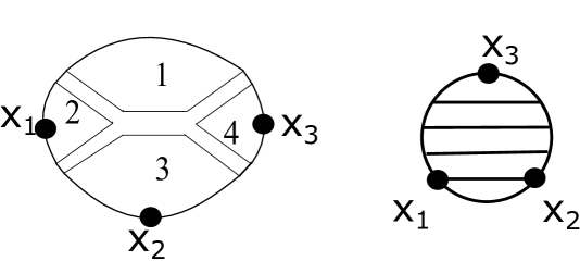
Figure 1. Critical ribbon graphs.

Definition 2.3.

A nodal ribbon graph with boundary is $G=\left(\coprod_{i}G_{i}\right)/N$, where

• $\iota_{i}\colon G_{i}\to\Sigma_{i}$ are ribbon graphs with boundary.

• $N\subset(\cup_{i}V_{BM}(G_{i}))\times(\cup_{i}V_{BM}(G_{i}))$ is a set of ordered pairs of boundary marked points $(v_{1},v_{2})$, $v_{1}\neq v_{2}$, of the $G_{i}$’s which we identify.

We require that

• $G$ is a connected graph,

• Elements of $N$ are disjoint as sets (without ordering).

After the identification of the vertices $v_{1}$ and $v_{2}$ the corresponding point in the graph is called a node. The vertex $v_{1}$ is called the legal side of the node and the vertex $v_{2}$ is called the illegal side of the node.

The set of edges $\mathop{\mathrm{Edges}}\nolimits(G)$ is composed of the internal edges of the $G_{i}$’s and of the boundary edges. The boundary edges are the boundary segments between successive vertices which are not the illegal sides of nodes. For any boundary edge $e$ we denote by $m(e)$ the number of the illegal sides of nodes lying on it. The boundary marked points of $G$ are the boundary marked points of $G_{i}$’s, which are not nodes. The set of boundary marked points of $G$ will be denoted by $V_{BM}(G)$ also in the nodal case.

A nodal graph $G=\left(\coprod_{i}G_{i}\right)/N$ is critical, if

• All of its components $G_{i}$ are critical.

• Ghost components do not contain the illegal sides of nodes.

It is called odd critical if it is critical and any boundary component of $G_{i}$ has an odd number of points that are the boundary marked points or the legal sides of nodes.

A graded (odd) critical nodal graph $(G,[K])$ is a critical (odd) ribbon graph with gradings associated to each component $G_{i}.$

A nodal ribbon graph with boundary is naturally embedded into the nodal surface $\Sigma=\left(\coprod_{i}\Sigma_{i}\right)/N$. The (doubled) genus of $\Sigma$ is called the genus of the graph. The notions of an isomorphism and metric are also as in the non-nodal case. Write $\mathcal{M}_{(G,[K])}$ for the moduli of metrics on $(G,[K]).$

Remark 2.4.

The genus of a closed, and in particular doubled, nodal surface $\Sigma$ is the genus of the smooth surface obtained by smoothing all nodes of $\Sigma.$

In Fig. 2 there is a critical nodal graph of genus $0$, with $5$ boundary marked points, $6$ internal marked points, three components, one of them is a ghost, two nodes, where a plus sign is drawn next to the legal side of a node and a minus sign is drawn next to the illegal side.

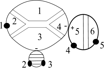
Figure 2. A critical nodal ribbon graph.

In Fig. 3 a non-critical nodal graph is shown. Here there is some vertex of degree $4,$ the components do not satisfy the parity condition and the ghost component has an illegal node.

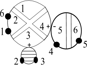
Figure 3. A non-critical nodal ribbon graph.

Let ${\mathcal{SR}}^{m}_{g,k,l}(\widetilde{\mathcal{SR}}^{m}_{g,k,l})$ be the set of isomorphism classes of graded (odd) critical nodal ribbon graphs with boundary of genus $g$, with $k$ boundary marked points, $l$ faces and together with a bijective labeling $\alpha:\mathop{\mathrm{Faces}}\nolimits(G)\stackrel{{\scriptstyle\sim}}{{\to}}[l]$, and $m$ nodes.

Denote by $\widetilde{\mathcal{R}}^{m}_{g,k,l}$ the set of isomorphism classes of odd critical nodal ribbon graphs with boundary of genus $g$, with $k$ boundary marked points, $l$ faces and together with a bijective labeling $\alpha:\mathop{\mathrm{Faces}}\nolimits(G)\stackrel{{\scriptstyle\sim}}{{\to}}[l],$ and $m$ nodes.

Definition 2.5.

An effective bridge in a graded critical graph $(G,[K])$ is a bridge $e$ with $m(e)=0.$ We denote their set by $Br^{eff}(G)$. The graph $\partial_{e}(G,[K])$, the result of contracting of the edge $e$ of $(G,[K]),$ which has one node $N$ more than $G$ has, can also be made critical nodal by declaring the side of $N$ which corresponds to $e$ to be legal, if $K(e)=0,$ and otherwise declare the other side of $N$ to be legal. Denote the resulting graph by $\mathcal{B}\partial_{e}(G,[K]).$ The operation $\mathcal{B}$ is called the base operation.

Definition 2.6.

For a metric graded ribbon graph $G,$ define

$$W_{G}:=\prod_{e\in\mathop{\mathrm{Edges}}\nolimits(G)}\frac{\ell_{e}^{2m(e)}}{(m(e)+1)!},\qquad\widetilde{W}_{G}:=\prod_{e\in\mathop{\mathrm{Edges}}\nolimits(G)}\frac{\ell_{e}^{2m(e)}}{m(e)!(m(e)+1)!}.$$

Definition 2.7.

An $l-$set is a map $L:[n]\to[l].$ The size of $L$ is $n.$ A subset of an $l-$set is the restriction map $L:A\to[l],~{}A\subseteq[n].$ It can canonically identified with a map $L^{\prime}:[|A|]\to[l],$ hence can be thought as an $l-$set on its own right. We write $L^{\prime}\subseteq L,$ and set $\binom{L}{m}$ for the set of all $\binom{n}{m}~{}l-$subsets of $L$ of size $m.$

Definition 2.8.

Any $l-$set defines a vector bundle $E_{L}:=\bigoplus\mathbb{L}_{L(i)},$ defined both on the moduli and on the combinatorial moduli. Let $S_{L}$ be the associated combinatorial sphere bundle. Let $\Phi_{L}$ be the associated explicit angular form, mentioned in Step $3$ above, and defined in [Tes15, Section 3]. Its curvature form is $\omega_{L}=\bigwedge_{i\in[n]}\omega_{L(i)}.$

Lemma 2.9.

Write $n=\frac{k+2l+3g-3}{2}$ Let $C\subseteq\mathcal{SR}_{g,k,l}^{m}$ be a set of graphs and let $C^{\prime}\subseteq\mathcal{SR}_{g,k,l}^{m+1}$ be the set of graphs obtained by applying for any graph in $C$ and any effective bridge $e$ of it, first the edge contraction $\partial_{e}$ and then the base operation $\mathcal{B}$. Suppose $C$ is closed in the following sense: for any graph $(G,[{K}])$ in $\mathcal{SR}_{g,k,l}^{m}\setminus C$ and any effective bridge $e$ of it we have $\mathcal{B}(\partial_{e}G)\notin C^{\prime}$. Then

$$\sum_{(G,[{K}])\in C}\sum_{e\in Br^{eff}(G)} \sum_{L^{\prime}\in\binom{L}{n-m}}\int_{\mathcal{M}_{\partial_{e}{(G,[{K}])}}}W_{G}\Phi_{L^{\prime}}=$$

$$=\sum_{(G,[{K}])\in C}\sum_{L^{\prime}\in\binom{L}{n-m-1}}\left(\int_{\mathcal{M}_{(G,[{K}])}}W_{G}\omega_{L^{\prime}}+\sum_{e\in Br^{eff}(G)}\int_{\mathcal{M}_{\partial_{e}{(G,[{K}])}}}W_{G}\Phi_{L^{\prime}}\right).$$

This lemma is the global version of the combination of Lemmas 6.7 and 6.8 of [Tes15] (there a local version is given, in terms of a single graph, rather than a set $C,$ and in terms of a single $l-$subset of it, rather than summing over all subsets).

Applying Lemma 2.9 iteratively to $C=\mathcal{SR}_{g,k,l}^{m},$ and using some parity observation (Proposition 6.13 in [Tes15]) give the integrated form of the combinatorial formula, [Tes15], Theorem 6.12.

Theorem 2.10.

For integers $a_{1},\ldots,a_{l}\geq 0$ which sum to $n=\frac{k+2l+3g-3}{2},$ let $L$ be any $l-$set with $E_{L}=\bigoplus\mathbb{L}_{i}^{\oplus a_{i}},$ then

$$2^{\frac{g+k-1}{2}}\langle\tau_{a_{1}}\cdots\tau_{a_{l}}\sigma^{k}\rangle^{o}_{g}=\sum_{m\geq 0}\sum_{(G,[{K}])\in\widetilde{\mathcal{SR}}_{g,k,l}^{m}}\sum_{L^{\prime}\in\binom{L}{n-m}}\int_{\mathcal{M}_{(G,[{K}])}(\mathbf{p})}W_{G}\omega_{L^{\prime}}.$$

A straightforward corollary is (equation (35) in [Tes15])

Corollary 2.11.

$$2^{\frac{g+k-1}{2}}\sum_{\sum_{i=1}^{l}a_{i}=n}\prod p_{i}^{2a_{i}}\langle\tau_{a_{1}}\cdots\tau_{a_{l}}\sigma^{k}\rangle^{o}_{g}=\sum_{m\geq 0}\sum_{(G,[{K}])\in\widetilde{\mathcal{SR}}_{g,k,l}^{m}}\sum_{L^{\prime}\in\binom{L}{n-m}}\int_{\mathcal{M}_{(G,[{K}])}(\mathbf{p})}\widetilde{W}_{G}\frac{\bar{\omega}^{n-m}}{(n-m)!},$$

where $\bar{\omega}=\sum_{i}p_{i}^{2}\omega_{i}.$

Note that in the last theorem and corollary there is no more dependence on the choice of the multisection.

Step 5. The last step is to perform Laplace transform to the integrated formula described above. This is the content of [Tes15, Sections 6.2, 6.3]. The only difficulty in the calculation of the Laplace transform of

$$\int_{\mathcal{M}_{(G,[{K}])}(\mathbf{p})}\widetilde{W}_{G}\frac{\bar{\omega}^{n-m}}{(n-m)!}$$

for a given $(G,[K])\in\widetilde{\mathcal{SR}}^{*}_{g,k,l}$ is to show

$$\bigwedge_{i=1}^{l}dp_{i}\wedge\frac{\bar{\omega}^{n-m}}{(n-m)!}:\bigwedge_{e\in\mathop{\mathrm{Edges}}\nolimits(G)}d\ell_{e}=\pm\prod_{i}2^{\frac{g(G_{i})+b(G_{i})-1}{2}+v_{I}(G_{i})},$$

and to understand the signs. Here $G_{i}$ are the components of $G$. This is the content of Section 6.2 in [Tes15].

After understanding the sign and the ratio of forms, the Laplace transform calculations are straightforward and give

(2.3) $$\int_{p_{i}\in\mathbb{R}_{+}}\bigwedge dp_{i}\exp{\left(-\sum\lambda_{i}p_{i}\right)}\int_{\mathcal{M}_{(G,[{K}])}(\mathbf{p})}\widetilde{W}_{G}\frac{\bar{\omega}^{n-m}}{(n-m)!}=\pm\frac{\prod_{i}2^{v_{I}(G_{i})+\frac{g(G_{i})+b(G_{i})-1}{2}}}{|\mathop{\mathrm{Aut}}\nolimits(G,[K])|}\prod_{e\in\mathop{\mathrm{Edges}}\nolimits(G)}\lambda(e),$$

where

(2.4) $$\lambda(e):=\begin{cases}\frac{1}{\lambda_{i}+\lambda_{j}},&\text{if $e$ is an internal edge between faces $i$ and $j$};\\ \frac{1}{(m+1)}\binom{2m}{m}\lambda_{i}^{-2m-1},&\text{if $e$ is a boundary edge of face $i$ and $m(e)=m$};\\ 1,&\text{if $e$ is a boundary edge of a ghost}.\end{cases}$$

Summing over the different gradings $K,$ and using the results of Section 6.2 regarding the signs give

(2.5) $$\sum_{[K]\text{ is a grading for G}}\int_{p_{i}\in\mathbb{R}_{+}}\bigwedge dp_{i}\exp{\left(-\sum\lambda_{i}p_{i}\right)}\int_{\mathcal{M}_{(G,[{K}])}(\mathbf{p})}\widetilde{W}_{G}\frac{\bar{\omega}^{n-m}}{(n-m)!}=\\ =\frac{\prod_{i}2^{v_{I}(G_{i})+\frac{g(G_{i})+b(G_{i})-1}{2}}}{|\mathop{\mathrm{Aut}}\nolimits(G)|}\prod_{e\in\mathop{\mathrm{Edges}}\nolimits(G)}\lambda(e).$$

Summing over all graphs, the resulting combinatorial formula is

Theorem 2.12.

Fix $g,k,l\geq 0$ such that $2g-2+k+2l>0$. Let $\lambda_{1},\ldots,\lambda_{l}$ be formal variables. Then we have

(2.6) $$2^{\frac{g+k-1}{2}}\sum_{a_{1},\ldots,a_{l}\geq 0}\langle\tau_{a_{1}}\tau_{a_{2}}\cdots\tau_{a_{l}}\sigma^{k}\rangle_{g}^{o}\prod_{i=1}^{l}\frac{2^{a_{i}}(2a_{i}-1)!!}{\lambda_{i}^{2a_{i}+1}}=\\ =\sum_{G=\left(\coprod_{i}G_{i}\right)/N\in\widetilde{\mathcal{R}}^{*}_{g,k,l}}\frac{\prod_{i}2^{v_{I}(G_{i})+g(G_{i})+b(G_{i})-1}}{|\mathop{\mathrm{Aut}}\nolimits(G)|}\prod_{e\in\mathop{\mathrm{Edges}}\nolimits(G)}\lambda(e).$$

2.2. A combinatorial formula for the refined and very refined numbers

In order to write a combinatorial formula for the more refined numbers, first note

Observation 2.13.

Let $(G^{\prime},[K^{\prime}])\in\mathcal{SR}^{m}_{g,k,l}$ be an arbitrary graph, then there exists a graph $(G,[K])\in\mathcal{SR}^{0}_{g,k,l},$ called the smoothing of $(G^{\prime},[K^{\prime}])$ and a sequence $(e_{j})_{j=1}^{m}$ of bridges of $G$ such that

$$\mathcal{B}\partial_{e_{m}}\cdots\mathcal{B}\partial_{e_{1}}(G,[K])=(G^{\prime},[K^{\prime}]).$$

Moreover, if $[\tilde{K}^{\prime}]$ is another graded structure on $G^{\prime}$ then the smoothing of $(G^{\prime},[\tilde{K}^{\prime}])$ is some $(G,[\tilde{K}])$ with the same $G.$ Thus, the number of boundaries and partitions of boundary points of the smoothing of a graph $(G^{\prime},[K^{\prime}])$ is well-defined and independent of the graded structure.

The proof is immediate, the operation $\mathcal{B}$ remembers the cyclic order of the illegal nodes on each boundary edge, hence remembers the topology of the graph on which $\mathcal{B}$ was applied. The edge contraction is easily inverted on the level of graphs, and the value of $K$ on the contracted bridge can be read from knowing which side of the node the $\mathcal{B}$ operation declared to be illegal. The second part of the observation follows from the fact that the different gradings on $G^{\prime}$ do not change the way we invert $\partial_{e}$.

Note that Steps 1–3 of the previous section work without change for the more refined numbers, giving us

(2.7) $$2^{\frac{g+k-1}{2}}\langle\tau_{a_{1}}\cdots\tau_{a_{l}}\sigma^{k}\rangle^{o}_{g,b}=\sum_{(G,z)\in\mathcal{SR}_{g,b,k,l}^{0}}\int_{\mathcal{M}_{(G,z)}(\mathbf{p})}\bigwedge_{i=1}^{l}\omega_{i}^{a_{i}}+\sum_{\begin{subarray}{c}(G,z)\in\mathcal{SR}_{g,b,k,l}^{0}\\ e\in Br(G)\end{subarray}}\int_{\mathcal{M}_{\partial_{e}(G,[K])}(\mathbf{p})}(s^{\prime})^{*}\Phi,$$

where $\mathcal{SR}_{g,b,k,l}^{m}$ is the subset of $\mathcal{SR}_{g,k,l}^{m}$ made of graphs whose smoothing has $b$ boundary components, and $s^{\prime}$ is again combinatorial canonical. Define similarly $\widetilde{\mathcal{SR}}^{m}_{g,b,k,l},\mathcal{R}^{m}_{g,b,k,l}$ and $\widetilde{\mathcal{R}}^{m}_{g,b,k,l}$. Define $\mathcal{SR}_{g,\bar{k},l}^{m},\widetilde{\mathcal{SR}}^{m}_{g,\overline{k},l},\mathcal{R}^{m}_{g,\overline{k},l},\widetilde{\mathcal{R}}^{m}_{g,\overline{k},l}$, accordingly, for graphs which correspond to a partition $\bar{k}$ of boundary marked points. Then acting similarly for the very refined numbers yields

(2.8) $$2^{\frac{g+k-1}{2}}\langle\tau_{a_{1}}\cdots\tau_{a_{l}}\sigma^{\bar{k}}\rangle^{o}_{g}=\sum_{(G,z)\in\mathcal{SR}_{g,\bar{k},l}^{0}}\int_{\mathcal{M}_{(G,z)}(\mathbf{p})}\bigwedge_{i=1}^{l}\omega_{i}^{a_{i}}+\sum_{\begin{subarray}{c}(G,z)\in\mathcal{SR}_{g,\bar{k},l}^{0}\\ e\in Br(G)\end{subarray}}\int_{\mathcal{M}_{\partial_{e}(G,[K])}(\mathbf{p})}(s^{\prime})^{*}\Phi,$$

where $s^{\prime}$ is again combinatorial canonical.

Step 4 requires some modification. Observation 2.13 allows us to apply Lemma 2.9 to the sets $C$ obtained by taking an arbitrary $(G,[K])\in\mathcal{SR}^{0}_{g,k,l}$ and creating all elements of $\mathcal{SR}^{m}_{g,k,l}$ obtained from it by contracting bridges and applying $\mathcal{B}.$

Using Lemma 2.9 iteratively now gives

Theorem 2.14.

For integers $a_{1},\ldots,a_{l}\geq 0$ which sum to $n=\frac{k+2l+3g-3}{2},$ let $L$ be any $l-$set with $E_{L}=\bigoplus\mathbb{L}_{i}^{\oplus a_{i}},$ then

$$2^{\frac{g+k-1}{2}}\langle\tau_{a_{1}}\cdots\tau_{a_{l}}\sigma^{k}\rangle^{o}_{g,b}=\sum_{m\geq 0}\sum_{(G,[{K}])\in\widetilde{\mathcal{SR}}_{g,b,k,l}^{m}}\sum_{L^{\prime}\in\binom{L}{n-m}}\int_{\mathcal{M}_{(G,[{K}])}(\mathbf{p})}W_{G}\omega_{L^{\prime}},$$

and

$$2^{\frac{g+k-1}{2}}\sum_{\sum_{i=1}^{l}a_{i}=n}\prod p_{i}^{2a_{i}}\langle\tau_{a_{1}}\cdots\tau_{a_{l}}\sigma^{k}\rangle^{o}_{g,b}=\sum_{m\geq 0}\sum_{(G,[{K}])\in\widetilde{\mathcal{SR}}_{g,b,k,l}^{m}}\sum_{L^{\prime}\in\binom{L}{n-m}}\int_{\mathcal{M}_{(G,[{K}])}(\mathbf{p})}\widetilde{W}_{G}\frac{\bar{\omega}^{n-m}}{(n-m)!},$$

where $\bar{\omega}=\sum_{i}p_{i}^{2}\omega_{i}$.

Similarly, under the same assumptions,

Theorem 2.15.

$$2^{\frac{g+k-1}{2}}\langle\tau_{a_{1}}\cdots\tau_{a_{l}}\sigma^{\bar{k}}\rangle^{o}_{g}=\sum_{m\geq 0}\sum_{(G,[{K}])\in\widetilde{\mathcal{SR}}_{g,\overline{k},l}^{m}}\sum_{L^{\prime}\in\binom{L}{n-m}}\int_{\mathcal{M}_{(G,[{K}])}(\mathbf{p})}W_{G}\omega_{L^{\prime}},$$

and

$$2^{\frac{g+k-1}{2}}\sum_{\sum_{i=1}^{l}a_{i}=n}\prod p_{i}^{2a_{i}}\langle\tau_{a_{1}}\cdots\tau_{a_{l}}\sigma^{\overline{k}}\rangle^{o}_{g}=\sum_{m\geq 0}\sum_{(G,[{K}])\in\widetilde{\mathcal{SR}}_{g,\overline{k},l}^{m}}\sum_{L^{\prime}\in\binom{L}{n-m}}\int_{\mathcal{M}_{(G,[{K}])}(\mathbf{p})}\widetilde{W}_{G}\frac{\bar{\omega}^{n-m}}{(n-m)!}.$$

Step 5 follows without change, since the Laplace transform is performed cell-by-cell, and then summed over gradings, we see that for the refined numbers it holds that

Theorem 2.16.

Fix $g,k,l\geq 0$ such that $2g-2+k+2l>0$. Let $\lambda_{1},\ldots,\lambda_{l}$ be formal variables. Then we have

(2.9) $$2^{\frac{g+k-1}{2}}\sum_{a_{1},\ldots,a_{l}\geq 0}\langle\tau_{a_{1}}\tau_{a_{2}}\cdots\tau_{a_{l}}\sigma^{k}\rangle_{g,b}^{o}\prod_{i=1}^{l}\frac{2^{a_{i}}(2a_{i}-1)!!}{\lambda_{i}^{2a_{i}+1}}=\\ =\sum_{G=\left(\coprod_{i}G_{i}\right)/N\in\widetilde{\mathcal{R}}^{*}_{g,b,k,l}}\frac{\prod_{i}2^{v_{I}(G_{i})+g(G_{i})+b(G_{i})-1}}{|\mathop{\mathrm{Aut}}\nolimits(G)|}\prod_{e\in\mathop{\mathrm{Edges}}\nolimits(G)}\lambda(e).$$

(2.10) $$2^{\frac{g+k-1}{2}}\sum_{a_{1},\ldots,a_{l}\geq 0}\langle\tau_{a_{1}}\tau_{a_{2}}\cdots\tau_{a_{l}}\sigma^{\bar{k}}\rangle_{g}^{o}\prod_{i=1}^{l}\frac{2^{a_{i}}(2a_{i}-1)!!}{\lambda_{i}^{2a_{i}+1}}=\\ =\sum_{G=\left(\coprod_{i}G_{i}\right)/N\in\widetilde{\mathcal{R}}^{*}_{g,\bar{k},l}}\frac{\prod_{i}2^{v_{I}(G_{i})+g(G_{i})+b(G_{i})-1}}{|\mathop{\mathrm{Aut}}\nolimits(G)|}\prod_{e\in\mathop{\mathrm{Edges}}\nolimits(G)}\lambda(e).$$

3. Matrix models

In this section we present matrix models for the very refined and the extended refined open partition functions and study their properties. In Section 3.1 we briefly recall the derivation of the matrix model for the open partition function $\tau^{o}$. Then in Section 3.2 we show how to modify it in order to control the distribution of boundary marked points on boundary components of a Riemann surface with boundary. As a result, we obtain a two-matrix model for the very refined open partition function $\widetilde{\tau}^{o}$. In Section 3.3 we give a construction of the extended refined open partition function $\tau^{o,ext}_{N}$ and present simple transformations that relate it to the function $\widetilde{\tau}^{o}$. In Section 3.4 we analyze the Feynman diagram expansion of the matrix integral for $\tau^{o,ext}_{N}$ and then in Sections 3.5, 3.6 derive the string and the dilaton equations for $\tau^{o,ext}_{N}$.

It will be useful for the future to rewrite formula (2.10) in the following way. For a graph $G=\left(\coprod_{i}G_{i}\right)/N\in\widetilde{\mathcal{R}}^{*}_{g,\overline{k},l}$ introduce a combinatorial constant $c(G)$ by $c(G):=\prod_{i}c(G_{i})$, where

(3.1) $$c(G_{i}):=\begin{cases}\frac{1}{2},&\text{if $G_{i}$ is a ghost},\\ 2^{e_{I}(G_{i})-v_{I}(G_{i})-v_{B3}(G_{i})-v_{BM}(G_{i})+b(G_{i})},&\text{otherwise},\end{cases}$$

and $e_{I}(G_{i})$ denotes the number of internal edges in $G_{i}$, $v_{B3}(G_{i})$ is the number of boundary trivalent vertices and $v_{BM}(G_{i})$ is the number of boundary marked points in $G_{i}$. Then for any $g,k,l\geq 0$, $b\geq 1$ and $\overline{k}\in P(k,b)$ we have

(3.2) $$\sum_{a_{1},\ldots,a_{l}\geq 0}\langle\tau_{a_{1}}\tau_{a_{2}}\cdots\tau_{a_{l}}\sigma^{\overline{k}}\rangle_{g}^{o}\prod_{i=1}^{l}\frac{(2a_{i}-1)!!}{\lambda_{i}^{2a_{i}+1}}=\sum_{G=\left(\coprod_{i}G_{i}\right)/N\in\widetilde{\mathcal{R}}^{*}_{g,\overline{k},l}}\frac{c(G)}{|\mathop{\mathrm{Aut}}\nolimits(G)|}\prod_{e\in\mathop{\mathrm{Edges}}\nolimits(G)}\lambda(e).$$

3.1. Open partition function

Let $M\geq 1$. Consider positive real numbers $\lambda_{1},\ldots,\lambda_{M}\in\mathbb{R}_{>0}$ and the diagonal matrix

$$\Lambda:=\mathop{\mathrm{diag}}\nolimits(\lambda_{1},\ldots,\lambda_{M}).$$

Let

$$c_{\Lambda,M}:=(2\pi)^{-\frac{M^{2}}{2}}\prod_{i=1}^{M}\sqrt{\lambda_{i}}\prod_{1\leq i<j\leq M}(\lambda_{i}+\lambda_{j}).$$

Denote by $\mathcal{H}_{M}$ the space of Hermitian $M\times M$ matrices. For a Hermitian matrix $H\in\mathcal{H}_{M}$ denote by $h_{i,j}$, $1\leq i,j\leq M$, its entries. Let

$$t_{i}(\Lambda):=(2i-1)!!\mathop{\mathrm{tr}}\nolimits\Lambda^{-2i-1},\quad i\geq 0.$$

We consider the standard volume form

$$dH:=\prod_{i=1}^{M}dh_{i,i}\prod_{1\leq i<j\leq M}d\left(\mathop{\mathrm{Re}}\nolimits{h}_{i,j}\right)d\left(\mathop{\mathrm{Im}}\nolimits{h}_{i,j}\right)$$

on $\mathcal{H}_{M}$. In [BT15] the second and the third authors proved that

(3.3) $$\left.\tau^{o}\right|_{t_{i}=t_{i}(\Lambda)}=\left.e^{\frac{\partial^{2}}{\partial s\partial s_{-}}}\left(e^{\frac{s^{3}}{6}}c_{\Lambda,M}\int_{\mathcal{H}_{M}}e^{\frac{1}{6}\mathop{\mathrm{tr}}\nolimits H^{3}-\frac{1}{2}\mathop{\mathrm{tr}}\nolimits H^{2}\Lambda}\det\frac{\Lambda+\sqrt{\Lambda^{2}-2s_{-}}-H+s}{\Lambda+\sqrt{\Lambda^{2}-2s_{-}}-H-s}dH\right)\right|_{s_{-}=0}.$$

The integral in the brackets on the right-hand side of this expression can be understood in the sense of formal matrix integration. The form

$$c_{\Lambda,M}e^{-\frac{1}{2}\mathop{\mathrm{tr}}\nolimits H^{2}\Lambda}dH$$

gives a Gaussian probability measure on $\mathcal{H}_{M}$. Then we can expand the function

$$e^{\frac{1}{6}\mathop{\mathrm{tr}}\nolimits H^{3}}\det\frac{\Lambda+\sqrt{\Lambda^{2}-2s_{-}}-H+s}{\Lambda+\sqrt{\Lambda^{2}-2s_{-}}-H-s}$$

in a series of the form

(3.4) $$\sum_{a,b,m\geq 0}s^{a}s_{-}^{b}P_{a,b,m},$$

where $P_{a,b,m}$ is a polynomial of degree $m$ in expressions of the form $\mathop{\mathrm{tr}}\nolimits(H\Lambda^{-d_{1}}H\Lambda^{-d_{2}}\cdots H\Lambda^{-d_{r}})$, $r\geq 1$. Here the degree is introduced by putting $\mathop{\mathrm{deg}}\nolimits(\mathop{\mathrm{tr}}\nolimits(H\Lambda^{-d_{1}}H\Lambda^{-d_{2}}\cdots H\Lambda^{-d_{r}})):=r+2\sum_{i=1}^{r}d_{i}$. Note that the integral

$$c_{\Lambda,N}\int_{\mathcal{H}_{N}}P_{a,b,m}e^{-\frac{1}{2}\mathop{\mathrm{tr}}\nolimits H^{2}\Lambda}dH$$

is zero, if $m$ is odd, and is a rational function in $\lambda_{1},\ldots,\lambda_{N}$ of degree $-\frac{m}{2}$, if $m$ is even. The integral on the right-hand side of (3.3) is understood as the term-wise integral of (3.4) with respect to our Gaussian probability measure on $\mathcal{H}_{M}$. We refer the reader to [BT15] for a more detailed discussion.

Let us briefly recall the derivation of formula (3.3). It is obtained from the combinatorial formula (2.6), rewritten similarly to (3.2), using the standard matrix models technique. An odd critical nodal ribbon graph with boundary can be obtained from the disjoint union of critical non-nodal ribbon graphs with boundary by gluing boundary marked points. Since the sides of each node of the nodal graph are marked by plus or minus, we should assign pluses and minuses to the boundary marked points of the critical non-nodal ribbon graphs with boundary. A collar neighborhood of a boundary component of a critical non-nodal ribbon graph with boundary, that is not a ghost, is a circle with ribbon half-edges attached to it and also with boundary marked points (see Fig. 4).

Figure 4. Boundary piece

Such a circle with a configuration of ribbon half-edges and marked points will be called a boundary piece. We see that our odd critical nodal ribbon graph with boundary is obtained by

• gluing a set of trivalent stars (see Fig. 5)

  Figure 5. Trivalent star and a ghost

  and boundary pieces,

• taking the disjoint union with a number of ghost components (see Fig. 5), and

• gluing each boundary marked point coming with minus to a boundary marked point coming with plus.

Remember also that, according to the definition of an odd critical nodal ribbon graph with boundary, the number of boundary marked points coming plus on each boundary piece should be odd. We obtain that the trivalent stars give the contribution $e^{\frac{1}{6}\mathop{\mathrm{tr}}\nolimits H^{3}}$ in the matrix model (3.3). Let

$$G(\Lambda,s_{-}):=\sum_{m\geq 0}\frac{2^{-m}}{m+1}{2m\choose m}s_{-}^{m}\Lambda^{-2m-1}=\frac{2}{\Lambda+\sqrt{\Lambda^{2}-2s_{-}}}.$$

Then boundary pieces give

$$\exp\left(\mathop{\mathrm{tr}}\nolimits\left[\sum_{k\geq 1}\frac{1}{k}\left(\frac{H+s}{2}G(\Lambda,s_{-})\right)^{k}-\sum_{k\geq 1}\frac{1}{k}\left(\frac{H-s}{2}G(\Lambda,s_{-})\right)^{k}\right]\right)=\det\frac{\Lambda+\sqrt{\Lambda^{2}-2s_{-}}-H+s}{\Lambda+\sqrt{\Lambda^{2}-2s_{-}}-H-s}.$$

The ghost components give the factor $e^{\frac{s^{3}}{6}}$ in (3.3). The application of the operator $e^{\frac{\partial^{2}}{\partial s\partial s_{-}}}$ and setting $s_{-}=0$ correspond to gluing each boundary marked point coming with minus to a boundary marked point coming with plus.

3.2. Very refined open partition function

Let us construct now a matrix model for the very refined open partition function $\widetilde{\tau}^{o}$. Let $N\geq 1$. In addition to the space $\mathcal{H}_{M}$ of Hermitian matrices, we consider the space $\mathrm{Mat}_{N,N}(\mathbb{C})$ of complex $N\times N$ matrices. We consider it as a real vector space of dimension $2N^{2}$. For a matrix $Z\in\mathrm{Mat}_{N,N}(\mathbb{C})$ denote by $z_{i,j}$, $1\leq i,j\leq N$, its entries. Define a volume form $dZ$ on $\mathrm{Mat}_{N,N}(\mathbb{C})$ by

$$dZ:=\prod_{1\leq i,j\leq N}d(\mathop{\mathrm{Re}}\nolimits z_{i,j})d(\mathop{\mathrm{Im}}\nolimits z_{i,j}).$$

Consider the Gaussian probability measure on $\mathrm{Mat}_{N,N}(\mathbb{C})$ given by the form

$$\frac{1}{(2\pi)^{N^{2}}}e^{-\frac{1}{2}\mathop{\mathrm{tr}}\nolimits Z\overline{Z}^{t}}dZ.$$

Let $\theta_{i,j}$, $1\leq i,j\leq N$, be complex variables and

$$\Theta:= (\theta_{i,j})_{1\leq i,j\leq N}\in\mathrm{Mat}_{N,N}(\mathbb{C}),$$

$$q_{m}(\Theta):= \mathop{\mathrm{tr}}\nolimits\Theta^{m},\quad m\geq 0.$$

Theorem 3.1.

We have

(3.5) $$\left.\widetilde{\tau}^{o}\right|_{\begin{subarray}{c}t_{i}=t_{i}(\Lambda)\\ q_{i}=q_{i}(\Theta)\end{subarray}}=\frac{c_{\Lambda,M}}{(2\pi)^{N^{2}}}\int_{\mathcal{H}_{M}\times\mathrm{Mat}_{N,N}(\mathbb{C})}e^{-\frac{1}{2}\mathop{\mathrm{tr}}\nolimits H^{2}\Lambda-\frac{1}{2}\mathop{\mathrm{tr}}\nolimits Z\overline{Z}^{t}}e^{\frac{1}{6}\mathop{\mathrm{tr}}\nolimits H^{3}+\frac{1}{6}\mathop{\mathrm{tr}}\nolimits Z^{3}+\frac{1}{2}\mathop{\mathrm{tr}}\nolimits\overline{Z}^{t}\Theta}\times$$

$$\hskip 113.81102pt\times\det\frac{\Lambda\otimes\mathrm{id}_{N}+\sqrt{\Lambda^{2}\otimes\mathrm{id}_{N}-\mathrm{id}_{M}\otimes\overline{Z}^{t}}-H\otimes\mathrm{id}_{N}+\mathrm{id}_{M}\otimes Z}{\Lambda\otimes\mathrm{id}_{N}+\sqrt{\Lambda^{2}\otimes\mathrm{id}_{N}-\mathrm{id}_{M}\otimes\overline{Z}^{t}}-H\otimes\mathrm{id}_{N}-\mathrm{id}_{M}\otimes Z}dHdZ.$$

Proof.

We now use the combinatorial formula (3.2). As we explained in the previous section, an odd critical nodal ribbon graph with boundary is obtained by gluing trivalent stars (Fig. 5) and boundary pieces (Fig. 4), adding ghost components (Fig. 5) and then gluing boundary points to create nodes. The problem now is to control the distribution of the boundary marked points on the boundary components in a smoothing the resulting nodal ribbon graph with boundary. Our idea is the following. Consider the nodal surface with boundary that is associated with our nodal ribbon graph with boundary. Consider a small neighborhood of a boundary node of this surface. At this node two small pieces of boundary components meet. Then, instead of gluing these two pieces at one point, we connect them by a small ribbon edge (see Fig. 6).

Figure 6. Inserting external ribbon edges

The new ribbon edge will be called an external ribbon edge. In Fig. 6 we fill the external ribbon edges by dots in order to distinguish them with the usual internal ribbon edges. Doing this procedure at each node, we obtain a non-nodal surface with boundary, which is a smoothing of the initial nodal surface. Note that each half of an external ribbon edge is marked by plus or minus.

Note that the resulting non-nodal surface can be glued from elementary pieces in the following way. Again we have trivalent stars (Fig. 5). Then we have boundary pieces similar to what we have in the previous section, but now we want to replace each boundary marked point by an external ribbon half-edge, marked by plus or minus (see Fig. 7).

Figure 7. Boundary piece with external ribbon half-edges

In the same way we replace the ghost component from Fig. 5 by the ghost component with external ribbon half-edges (see Fig. 8).

Figure 8. Ghost component with external ribbon half-edges

In order to have marked points we have to introduce an external ribbon half-edge marked by minus (see Fig. 9).

Figure 9. External ribbon half-edge corresponding to a marked point

Now, in order to obtain our non-nodal surface with external ribbon edges, we glue a set of elementary pieces of four types (Fig. 5, 7, 8, 9) according to the following rules:

• An internal ribbon half-edge should be glued to an internal ribbon half-edge.

• An external ribbon half-edge with some sign should be glued to an external ribbon half-edge with an opposite sign.

For a polynomial $P(Z)\in\mathbb{C}[z_{ij},\overline{z}_{kl}]$ let

$$\left<P(Z)\right>:=\frac{1}{(2\pi)^{N^{2}}}\int P(Z)e^{-\frac{1}{2}\mathop{\mathrm{tr}}\nolimits Z\overline{Z}^{t}}dZ.$$

Then we have

(3.6) $$\left<z_{i,j},z_{k,l}\right>=\left<\overline{z}_{i,j},\overline{z}_{k,l}\right>=0,$$

(3.7) $$\left<z_{i,j},\overline{z}_{k,l}\right>=2\delta_{i,k}\delta_{j,l}.$$

Formulas (3.6) and (3.7) show that our Gaussian probability measure on $\mathrm{Mat}_{N,N}(\mathbb{C})$ is the correct measure to control gluings of external ribbon half-edges with signs. To each elementary piece from Fig. 5, 7, 8, 9 we assign a function on $\mathcal{H}_{M}\times\mathrm{Mat}_{N,N}(\mathbb{C})$ in the way shown on these figures. Only the case of boundary pieces with external ribbon half-edges needs explanations. The function, corresponding to such a piece, is the product of a function on $\mathcal{H}_{M}$ and a function on $\mathrm{Mat}_{N,N}(\mathbb{C})$. The function of $\mathcal{H}_{M}$ is obtained in the same way as in the previous section with the only difference that we forget about the variables $s$ and $s_{-}$. Concerning a function on $\mathrm{Mat}_{N,N}(\mathbb{C})$, we go around the boundary piece in the clockwise direction and look at the external ribbon half-edges that we meet. If an external ribbon half-edge is marked by plus then we assign to it the matrix $Z$ and if it is marked by minus then we assign to it the matrix $\overline{Z}^{t}$. Then the function on $\mathrm{Mat}_{N,N}(\mathbb{C})$ is the trace of the product of these matrices taken according to their order in the clockwise direction. So, the resulting function on $\mathcal{H}_{M}\times\mathrm{Mat}_{N,N}(\mathbb{C})$ is the product of two traces. Note that the product of the traces of two matrices is the trace of their tensor product. We obtain that all boundary pieces with external ribbon half-edges give the following contribution to the matrix model for $\widetilde{\tau}^{o}$:

(3.8) $$\exp\left(\mathop{\mathrm{tr}}\nolimits\left[\sum_{k\geq 1}\frac{1}{k}\left(\frac{H\otimes\mathrm{id}_{N}+\mathrm{id}_{M}\otimes Z}{2}G(\Lambda,\overline{Z}^{t})\right)^{k}-\sum_{k\geq 1}\frac{1}{k}\left(\frac{H\otimes\mathrm{id}_{N}-\mathrm{id}_{M}\otimes Z}{2}G(\Lambda,\overline{Z}^{t})\right)^{k}\right]\right),$$

where $\mathrm{id}_{M}$ and $\mathrm{id}_{N}$ are the identity matrices in the spaces $\mathcal{H}_{M}$ and $\mathrm{Mat}_{N,N}(\mathbb{C})$, respectively, and

$$G(\Lambda,\overline{Z}^{t}):=\sum_{m\geq 0}\frac{2^{-2m}}{m+1}{2m\choose m}\Lambda^{-2m-1}\otimes(\overline{Z}^{t})^{m}=\frac{2}{\Lambda\otimes\mathrm{id}_{N}+\sqrt{\Lambda^{2}\otimes\mathrm{id}_{N}-\mathrm{id}_{M}\otimes\overline{Z}^{t}}}.$$

We see that the expression (3.8) is equal to

$$\det\frac{\Lambda\otimes\mathrm{id}_{N}+\sqrt{\Lambda^{2}\otimes\mathrm{id}_{N}-\mathrm{id}_{M}\otimes\overline{Z}^{t}}-H\otimes\mathrm{id}_{N}+\mathrm{id}_{M}\otimes Z}{\Lambda\otimes\mathrm{id}_{N}+\sqrt{\Lambda^{2}\otimes\mathrm{id}_{N}-\mathrm{id}_{M}\otimes\overline{Z}^{t}}-H\otimes\mathrm{id}_{N}-\mathrm{id}_{M}\otimes Z}.$$

Finally, the trivalent stars give the contribution $e^{\frac{1}{6}\mathop{\mathrm{tr}}\nolimits H^{3}}$ in the matrix model (3.5), the ghost components with external ribbon half-edges give $e^{\frac{1}{6}\mathop{\mathrm{tr}}\nolimits Z^{3}}$ and the external ribbon half-edges corresponding to marked points give $e^{\frac{1}{2}\mathop{\mathrm{tr}}\nolimits\overline{Z}^{t}\Theta}$. The theorem is proved. ∎

Using this theorem, we can obtain a matrix model for the refined open partition function $\tau^{o}_{N}$ in the following way:

(3.9) $$\left.\tau^{o}_{N}\right|_{t_{i}=t_{i}(\Lambda)}=\left.\left(\left.\widetilde{\tau}^{o}\right|_{\begin{subarray}{c}t_{i}=t_{i}(\Lambda)\\ q_{i}=q_{i}(\Theta)\end{subarray}}\right)\right|_{\Theta=s\,\mathrm{id}_{N}}=$$

$$= \frac{c_{\Lambda,M}}{(2\pi)^{N^{2}}}\int_{\mathcal{H}_{M}\times\mathrm{Mat}_{N,N}(\mathbb{C})}e^{-\frac{1}{2}\mathop{\mathrm{tr}}\nolimits H^{2}\Lambda-\frac{1}{2}\mathop{\mathrm{tr}}\nolimits Z\overline{Z}^{t}}e^{\frac{1}{6}\mathop{\mathrm{tr}}\nolimits H^{3}+\frac{1}{6}\mathop{\mathrm{tr}}\nolimits Z^{3}+\frac{s}{2}\mathop{\mathrm{tr}}\nolimits\overline{Z}^{t}}\times$$

$$\hskip 56.9055pt\times\det\frac{\Lambda\otimes\mathrm{id}_{N}+\sqrt{\Lambda^{2}\otimes\mathrm{id}_{N}-\mathrm{id}_{M}\otimes\overline{Z}^{t}}-H\otimes\mathrm{id}_{N}+\mathrm{id}_{M}\otimes Z}{\Lambda\otimes\mathrm{id}_{N}+\sqrt{\Lambda^{2}\otimes\mathrm{id}_{N}-\mathrm{id}_{M}\otimes\overline{Z}^{t}}-H\otimes\mathrm{id}_{N}-\mathrm{id}_{M}\otimes Z}dHdZ.$$

3.3. Extended refined open partition function

The extended open partition function $\tau^{o,ext}\in\mathbb{Q}[[t_{0},t_{1},\ldots,s_{0},s_{1},\ldots]]$, introduced in [Bur15, Bur16], is uniquely determined by the following equations:

(3.10) $$\left.\tau^{o,ext}\right|_{s_{\geq 1}=0}=\tau^{o},$$

(3.11) $$\frac{\partial}{\partial s_{n}}\tau^{o,ext}=\frac{1}{(n+1)!}\frac{\partial^{n+1}}{\partial s^{n+1}}\tau^{o,ext},\qquad n\geq 0.$$

Note that equation (3.9) gives a formula for $\tau^{o}$ that is slightly different to the initial formula (3.3),

(3.12) $$\left.\tau^{o}\right|_{t_{i}=t_{i}(\Lambda)}=\frac{c_{\Lambda,M}}{2\pi}\int_{\mathcal{H}_{M}\times\mathbb{C}}e^{-\frac{1}{2}\mathop{\mathrm{tr}}\nolimits H^{2}\Lambda-\frac{1}{2}z\overline{z}}e^{\frac{1}{6}\mathop{\mathrm{tr}}\nolimits H^{3}+\frac{z^{3}}{6}+\frac{1}{2}s\overline{z}}\det\frac{\Lambda+\sqrt{\Lambda^{2}-\overline{z}}-H+z}{\Lambda+\sqrt{\Lambda^{2}-\overline{z}}-H-z}dHd^{2}z,$$

where $d^{2}z:=d(\mathop{\mathrm{Re}}\nolimits z)d(\mathop{\mathrm{Im}}\nolimits z)$. Formulas (3.10) and (3.11) imply that

$$\left.\tau^{o,ext}\right|_{t_{i}=t_{i}(\Lambda)}=$$

$$= \frac{c_{\Lambda,M}}{2\pi}\int_{\mathcal{H}_{M}\times\mathbb{C}}e^{-\frac{1}{2}\mathop{\mathrm{tr}}\nolimits H^{2}\Lambda-\frac{z\overline{z}}{2}}e^{\frac{1}{6}\mathop{\mathrm{tr}}\nolimits H^{3}+\frac{z^{3}}{6}}\det\frac{\Lambda+\sqrt{\Lambda^{2}-\overline{z}}-H+z}{\Lambda+\sqrt{\Lambda^{2}-\overline{z}}-H-z}e^{\sum_{i\geq 0}\frac{2^{-i-1}}{(i+1)!}s_{i}\overline{z}^{i+1}}dHd^{2}z.$$

Let

$$s_{i}(\Lambda):=2^{i}i!\mathop{\mathrm{tr}}\nolimits\Lambda^{-2i-2},\quad i\geq 0.$$

It is easy to see that

$$\left.e^{\sum_{i\geq 0}\frac{2^{-i-1}}{(i+1)!}s_{i}\overline{z}^{i+1}}\right|_{s_{i}=s_{i}(\Lambda)}= e^{\frac{1}{2}\sum_{i\geq 0}\frac{\overline{z}^{i+1}}{(i+1)}\mathop{\mathrm{tr}}\nolimits\Lambda^{-2i-2}}=e^{-\frac{1}{2}\mathop{\mathrm{tr}}\nolimits\log(1-\overline{z}\Lambda^{-2})}=$$

$$= \det\frac{1}{\sqrt{1-\overline{z}\Lambda^{-2}}}=\frac{\det\Lambda}{\det\sqrt{\Lambda^{2}-\overline{z}}}.$$

So, we get

(3.13) $$\left.\tau^{o,ext}\right|_{\begin{subarray}{c}t_{i}=t_{i}(\Lambda)\\ s_{i}=s_{i}(\Lambda)\end{subarray}}=$$

$$= \frac{c_{\Lambda,M}}{2\pi}\int_{\mathcal{H}_{M}\times\mathbb{C}}e^{-\frac{1}{2}\mathop{\mathrm{tr}}\nolimits H^{2}\Lambda-\frac{z\overline{z}}{2}}e^{\frac{1}{6}\mathop{\mathrm{tr}}\nolimits H^{3}+\frac{z^{3}}{6}}\det\frac{\Lambda+\sqrt{\Lambda^{2}-\overline{z}}-H+z}{\Lambda+\sqrt{\Lambda^{2}-\overline{z}}-H-z}\frac{\det\Lambda}{\det\sqrt{\Lambda^{2}-\overline{z}}}dHd^{2}z.$$

This formula together with equation (3.9) motivates us to introduce a formal power series $\tau^{o,ext}_{N}\in\mathbb{C}[[t_{0},t_{1},\ldots,s_{0},s_{1},\ldots]]$ by

(3.14) $$\left.\tau^{o,ext}_{N}\right|_{\begin{subarray}{c}t_{i}=t_{i}(\Lambda)\\ s_{i}=s_{i}(\Lambda)\end{subarray}}=\frac{c_{\Lambda,M}}{(2\pi)^{N^{2}}}\int_{\mathcal{H}_{M}\times\mathrm{Mat}_{N,N}(\mathbb{C})}e^{-\frac{1}{2}\mathop{\mathrm{tr}}\nolimits H^{2}\Lambda-\frac{1}{2}\mathop{\mathrm{tr}}\nolimits Z\overline{Z}^{t}}e^{\frac{1}{6}\mathop{\mathrm{tr}}\nolimits H^{3}+\frac{1}{6}\mathop{\mathrm{tr}}\nolimits Z^{3}}\times$$

$$\times\det\frac{\Lambda\otimes\mathrm{id}_{N}+\sqrt{\Lambda^{2}\otimes\mathrm{id}_{N}-\mathrm{id}_{M}\otimes\overline{Z}^{t}}-H\otimes\mathrm{id}_{N}+\mathrm{id}_{M}\otimes Z}{\Lambda\otimes\mathrm{id}_{N}+\sqrt{\Lambda^{2}\otimes\mathrm{id}_{N}-\mathrm{id}_{M}\otimes\overline{Z}^{t}}-H\otimes\mathrm{id}_{N}-\mathrm{id}_{M}\otimes Z}\frac{\det\Lambda^{N}dHdZ}{\det\sqrt{\Lambda^{2}\otimes\mathrm{id}_{N}-\mathrm{id}_{M}\otimes\overline{Z}^{t}}}.$$

The uniqueness of a power series with this property is obvious. However, the existence of such a series is not trivial. In order to prove it we will define a formal power series $\tau^{o,ext}_{N}$ using the function $\widetilde{\tau}^{o}$ and then prove that it satisfies equation (3.14).

For a given $N\geq 1$ let us define a formal power series $\tau^{o,ext}_{N}\in\mathbb{Q}[[t_{0},t_{1},\ldots,s_{0},s_{1},\ldots]]$ by

(3.15) $$\tau^{o,ext}_{N}(t_{0},t_{1},\ldots,s_{0},s_{1},\ldots):=\frac{1}{(2\pi)^{N^{2}}}\int_{\mathrm{Mat}_{N,N}(\mathbb{C})}\left.\widetilde{\tau}^{o}\right|_{q_{i}=q_{i}(Z)}e^{\sum_{i\geq 0}\frac{2^{-i-1}}{(i+1)!}s_{i}\mathop{\mathrm{tr}}\nolimits(\overline{Z}^{t})^{i+1}}e^{-\frac{1}{2}\mathop{\mathrm{tr}}\nolimits Z\overline{Z}^{t}}dZ.$$

Lemma 3.2.

The function $\tau^{o,ext}_{N}$ satisfies equation (3.14).

Proof.

Note that

(3.16) $$\frac{\det\Lambda^{N}}{\det\sqrt{\Lambda^{2}\otimes\mathrm{id}_{N}-\mathrm{id}_{M}\otimes\overline{Z}^{t}}}=\frac{1}{\det\sqrt{\mathrm{id}_{M}\otimes\mathrm{id}_{N}-\Lambda^{-2}\otimes\overline{Z}^{t}}}=e^{\sum_{i\geq 0}\frac{2^{-i-1}}{(i+1)!}s_{i}(\Lambda)\mathop{\mathrm{tr}}\nolimits(\overline{Z}^{t})^{i+1}}.$$

Then the lemma follows from Theorem 3.1 and the elementary formula:

$$\frac{1}{(2\pi)^{N^{2}}}\int_{\mathrm{Mat}_{N,N}(\mathbb{C})}Q(\Theta)e^{\frac{1}{2}\mathop{\mathrm{tr}}\nolimits\overline{Z}^{t}\Theta}e^{-\frac{1}{2}\mathop{\mathrm{tr}}\nolimits\Theta\overline{\Theta}^{t}}d\Theta=Q(Z),$$

where $Q(\Theta)\in\mathbb{C}[\overline{\theta}_{i,j}]$ is an arbitrary polynomial. ∎

For a finite value of $N$ the transform, defined by the right hand side of (3.15) is not invertible. However, if we know $\tau^{o,ext}_{N}$ for all $N\geq 1$, we can find $\widetilde{\tau}^{o}$. Let us consider the space ${\mathcal{U}}_{N}$ of unitary $N\times N$ matrices. Then we introduce the volume form on ${\mathcal{U}}_{N}$, which is proportional to the Haar measure and normalized by

$$\int_{{\mathcal{U}}_{N}}dU=1.$$

Let $p_{1},p_{2},\ldots$ and $p_{1}^{\prime},p_{2}^{\prime},\ldots$ be formal variables.

Lemma 3.3.

If

$$f_{N}(p^{\prime}_{1},p^{\prime}_{2},\dots):=\frac{1}{(2\pi)^{N^{2}}}\int_{\mathrm{Mat}_{N,N}(\mathbb{C})}\left.g\right|_{p_{i}=\frac{1}{i}\mathop{\mathrm{tr}}\nolimits Z^{i}}e^{\sum_{i\geq 1}2^{-i}p^{\prime}_{i}\mathop{\mathrm{tr}}\nolimits(\overline{Z}^{t})^{i}}e^{-\frac{1}{2}\mathop{\mathrm{tr}}\nolimits Z\overline{Z}^{t}}dZ$$

for some $g\in\mathbb{C}[[p_{1},p_{2},\dots]]$, then

$$\left.g\right|_{p_{i}=\frac{1}{i}\mathop{\mathrm{tr}}\nolimits A^{i}}=\int_{{\mathcal{U}}_{N}}\left.f_{N}\right|_{p^{\prime}_{i}=\frac{1}{i}\mathop{\mathrm{tr}}\nolimits U^{i}}e^{\mathop{\mathrm{tr}}\nolimits{\overline{U}}^{t}A}dU,\quad A\in\mathrm{Mat}_{N,N}(\mathbb{C}).$$

Proof.

The Schur functions $s_{\lambda}(p_{1},p_{2},\dots)$, labeled by partitions $\lambda=\{\lambda_{1}\geq\lambda_{2}\geq\lambda_{3}\geq\dots\}$, constitute a basis in the space of formal series in the variables $p_{1},p_{2},\dots$. Recall that they can be defined by

$$s_{\lambda}:=\det(h_{\lambda_{i}-i+j})_{1\leq i,j\leq l(\lambda)},$$

where the polynomials $h_{k}(p_{1},p_{2},\ldots)$, $k\in\mathbb{Z}$, are defined by

$$\sum_{i\geq 0}h_{i}z^{i}=e^{\sum_{i\geq 1}p_{i}z^{i}}$$

for $k\geq 0$ and by $h_{k}:=0$ for $k<0$. Thus, it is enough to prove the lemma for $g=s_{\lambda}$, where $l(\lambda)\leq N$. (If $l(\lambda)>N$ then both $\left.g\right|_{p_{i}=\frac{1}{i}\mathop{\mathrm{tr}}\nolimits Z^{i}}$ and $f_{N}$ are equal to zero.) For any matrix $A\in\mathrm{Mat}_{N,N}(\mathbb{C})$ let

$$p_{i}(A):=\frac{1}{i}\mathop{\mathrm{tr}}\nolimits A^{i},\quad i\geq 1.$$

For any partition $\mu$ and matrices $A,B\in\mathrm{Mat}_{N,N}(\mathbb{C})$ we have the following formula [Ale11, eq. (39)],

$$\frac{1}{(2\pi)^{N^{2}}}\int_{\mathrm{Mat}_{N,N}(\mathbb{C})}s_{\lambda}(p_{*}(ZA))s_{\mu}\left(p_{*}\left(\frac{1}{2}\overline{Z}^{t}B\right)\right)e^{-\frac{1}{2}\mathop{\mathrm{tr}}\nolimits Z\overline{Z}^{t}}dZ=\frac{s_{\lambda}(p_{*}(AB))}{s_{\lambda}(1,0,0,\ldots)}\delta_{\lambda,\mu}.$$

Then for any unitary matrix $U$ we can compute

$$\frac{1}{(2\pi)^{N^{2}}}\int_{\mathrm{Mat}_{N,N}(\mathbb{C})}s_{\lambda}(p_{*}(Z))e^{-\frac{1}{2}\mathop{\mathrm{tr}}\nolimits Z\overline{Z}^{t}+\sum_{i\geq 1}\frac{2^{-i}}{i}\mathop{\mathrm{tr}}\nolimits U^{i}\mathop{\mathrm{tr}}\nolimits(\overline{Z}^{t})^{i}}dZ=$$

$$= \frac{1}{(2\pi)^{N^{2}}}\int_{\mathrm{Mat}_{N,N}(\mathbb{C})}s_{\lambda}(p_{*}(Z))\sum_{\mu}s_{\mu}(p_{*}(U))s_{\mu}\left(p_{*}\left(1/2\overline{Z}^{t}\right)\right)e^{-\frac{1}{2}\mathop{\mathrm{tr}}\nolimits Z\overline{Z}^{t}}dZ=$$

$$= \frac{s_{\lambda}(p_{*}(\mathrm{id}_{N}))}{s_{\lambda}(1,0,0,\ldots)}s_{\lambda}(p_{*}(U))\stackrel{{\scriptstyle\text{\cite[cite]{[\@@bibref{}{Ale11}{}{}, Sec. 1.1]}}}}{{=}}C_{N}(\lambda)s_{\lambda}(p_{*}(U)),$$

where

$$C_{N}(\lambda)=\prod_{i=1}^{N}\frac{(\lambda_{i}+N-i)!}{(N-i)!}.$$

On the other hand, for any partition $\mu$ and matrices $A,B\in\mathrm{Mat}_{N,N}(\mathbb{C})$ we have [Ale11, eq. (31)]

$$\int_{\mathcal{U}_{N}}s_{\lambda}(p_{*}(UA))s_{\mu}(p_{*}(\overline{U}^{t}B))dU=\frac{s_{\lambda}(p_{*}(AB))}{s_{\lambda}(p_{*}(\mathrm{id}_{N}))}\delta_{\lambda,\mu}.$$

Therefore, we obtain

$$\int_{{\mathcal{U}}_{N}}s_{\lambda}(p_{*}(U))e^{\mathop{\mathrm{tr}}\nolimits\overline{U}^{t}A}dU=\int_{{\mathcal{U}}_{N}}s_{\lambda}(p_{*}(U))\sum_{k\geq 0}\frac{p_{1}(\overline{U}^{t}A)^{k}}{k!}dU=$$

$$= \int_{{\mathcal{U}}_{N}}s_{\lambda}(p_{*}(U))\sum_{\mu}s_{\mu}(1,0,0,\ldots)s_{\mu}(p_{*}(\overline{U}^{t}A))dU=\frac{1}{C_{N}(\lambda)}s_{\lambda}(p_{*}(A)).$$

This completes the proof of the lemma. ∎

In particular, we have

$$\left.\widetilde{\tau}^{o}\right|_{q_{i}=q_{i}(A)}=\int_{{\mathcal{U}}_{N}}\left.\tau^{o,ext}_{N}\right|_{s_{i}=i!\mathop{\mathrm{tr}}\nolimits U^{i+1}}e^{\mathop{\mathrm{tr}}\nolimits{\overline{U}}^{t}A}dU.$$

Equations (3.9), (3.13), (3.14) and (3.16) imply that

$$\left.\tau^{o,ext}_{N}\right|_{s_{\geq 1}=0}=\tau^{o}_{N},\qquad\tau^{o,ext}_{1}=\tau^{o,ext}.$$

We conjecture that there exists a geometric construction of boundary descendents in the refined open intersection theory giving the extended refined open partition function $\tau^{o,ext}_{N}$.

The function

$$F^{o,ext,N}:=\log\tau^{o,ext}_{N}-F^{c}$$

will be called the extended refined open free energy.

3.4. Feynman diagram expansion of the extended matrix model

Introduce the extended refined open intersection numbers by

(3.17) $$\left<\tau_{a_{1}}\cdots\tau_{a_{l}}\sigma_{c_{1}}\cdots\sigma_{c_{k}}\right>^{o,ext,N}:=\left.\frac{\partial^{l+k}F^{o,ext,N}}{\partial t_{a_{1}}\cdots\partial t_{a_{l}}\partial s_{c_{1}}\cdots\partial s_{c_{k}}}\right|_{t_{*}=s_{*}=0}.$$

From (3.15) it follows that the intersection number $\left<\tau_{a_{1}}\cdots\tau_{a_{l}}\sigma_{c_{1}}\cdots\sigma_{c_{k}}\right>^{o,ext,N}$ is actually a polynomial in $N$ with rational coefficients. So, it is well-defined for all values of $N$, not necessarily positive integers. Therefore, the extended refined open partition function $\tau^{o,ext}_{N}$ is also well-defined for all values of $N$. We want to write a combinatorial formula for the extended refined open intersection numbers similar to (2.9). Let us write the matrix model (3.14) for $\tau^{o,ext}_{N}$ in the following way:

(3.18) $$\left.\tau^{o,ext}_{N}\right|_{t_{i}=t_{i}(\Lambda)}=\frac{c_{\Lambda,M}}{(2\pi)^{N^{2}}}\int_{\mathcal{H}_{M}\times\mathrm{Mat}_{N,N}(\mathbb{C})}e^{-\frac{1}{2}\mathop{\mathrm{tr}}\nolimits H^{2}\Lambda-\frac{1}{2}\mathop{\mathrm{tr}}\nolimits Z\overline{Z}^{t}}e^{\frac{1}{6}\mathop{\mathrm{tr}}\nolimits H^{3}+\frac{1}{6}\mathop{\mathrm{tr}}\nolimits Z^{3}}\times$$

$$\times\det\frac{\Lambda\otimes\mathrm{id}_{N}+\sqrt{\Lambda^{2}\otimes\mathrm{id}_{N}-\mathrm{id}_{M}\otimes\overline{Z}^{t}}-H\otimes\mathrm{id}_{N}+\mathrm{id}_{M}\otimes Z}{\Lambda\otimes\mathrm{id}_{N}+\sqrt{\Lambda^{2}\otimes\mathrm{id}_{N}-\mathrm{id}_{M}\otimes\overline{Z}^{t}}-H\otimes\mathrm{id}_{N}-\mathrm{id}_{M}\otimes Z}e^{\sum_{i\geq 0}\frac{2^{-i-1}}{(i+1)!}s_{i}\mathop{\mathrm{tr}}\nolimits(\overline{Z}^{t})^{i+1}}dHdZ.$$

We see that this matrix model is obtained from (3.9) simply by adding the factor $e^{\sum_{i\geq 1}\frac{2^{-i-1}}{(i+1)!}s_{i}\mathop{\mathrm{tr}}\nolimits(\overline{Z}^{t})^{i+1}}$ in the integrand. Doing the Feynman diagram expansion of (3.18) one can easily see that there is a combinatorial formula for the intersection numbers (3.17) similar to (2.9), where we allow odd critical nodal ribbon graphs with boundary to have certain exceptional components. Let us formulate it precisely.

Recall that a $(g,k,l)$-ribbon graph with boundary is called critical, if

• Boundary marked points have degree $2$.

• All other vertices have degree $3$.

• If $l=0$, then $g=0$ and $k=3$.

We will call a $(g,k,l)$-ribbon graph with boundary exceptional, if $g=l=0$ and $k\geq 1$. Obviously, for each $k\geq 1$ there exists a unique such graph up to an isomorphism, see Fig. 10.

Figure 10. Exceptional graph and the corresponding diagram for the extended matrix model

Note, that we step back a little bit from the original definition of a ribbon graph with boundary, because exceptional graphs with $k=1$ or $k=2$ are strictly speaking not stable. Note also that a critical $(0,3,0)$-ribbon graph with boundary, that we call a ghost, coincides with an exceptional graph with $k=3$. However, our idea is to distinguish them. Speaking formally, to a $(0,3,0)$-ribbon graph with boundary we additionally assign a type: it can be a ghost or an exceptional graph. Using this terminology, the set of critical ribbon graphs with boundary does not intersect the set of exceptional graphs.

A nodal ribbon graph with boundary $G=\left(\coprod_{i}G_{i}\right)/N$ will be called extended critical, if

• It does not have boundary marked points.

• All of its components $G_{i}$ are critical or exceptional.

• Ghost components do not contain the illegal sides of nodes.

• Exceptional components do not contain the legal sides of nodes.

The fact, that we do not allow boundary marked points now, may look surprising, but one can note that an exceptional component with $k=1$ can be easily interpreted as a boundary marked point. An extended critical nodal ribbon graph with boundary $G=\left(\coprod_{i}G_{i}\right)/N$ is called odd if any boundary component of each non-exceptional $G_{i}$ has an odd number of the legal sides of nodes. Denote by $\widetilde{\mathcal{R}}^{ext}_{l}$ the set of odd extended critical nodal ribbon graphs with boundary with $l$ internal faces. For a graph $G=\left(\coprod_{i}G_{i}\right)/N\in\widetilde{\mathcal{R}}^{ext}_{l}$ introduce the following notations. Denote by $b(G)$ the number of boundary components in a smoothing of the nodal surface associated with $G$. Let $c(G):=\prod_{i}c(G_{i})$, where $c(G_{i})$ is defined by (3.1) if $G_{i}$ is non-exceptional and

$$c(G_{i}):=\frac{1}{m!},\quad\text{if $G_{i}$ is an exceptional graph with $m+1$ boundary vertices, $m\geq 0$}.$$

For $m\geq 0$ denote by $\mathrm{exc}_{m}(G)$ the number of exceptional components $G_{i}$ with exactly $m+1$ boundary vertices. The set of edges $\mathop{\mathrm{Edges}}\nolimits(G)$ is composed of the internal edges of the $G_{i}$’s and of the boundary edges. The boundary edges are the boundary segments in non-exceptional $G_{i}$’s between successive legal sides of nodes. For an edge $e\in\mathop{\mathrm{Edges}}\nolimits(G)$ the function $\lambda(e)$ is defined by the old formula (2.4). The Feynman diagram expansion of the matrix model (3.18) gives the following formula for the intersection numbers (3.17):

(3.19) $$\sum_{a_{1},\ldots,a_{l}\geq 0}\sum_{m\geq 0}\sum_{c_{1},\ldots,c_{m}\geq 0}\left<\tau_{a_{1}}\cdots\tau_{a_{l}}\sigma_{c_{1}}\cdots\sigma_{c_{m}}\right>^{o,ext,N}\prod_{i=1}^{l}\frac{(2a_{i}-1)!!}{\lambda_{i}^{2a_{i}+1}}\frac{\prod_{j=1}^{m}s_{c_{j}}}{m!}=\\ =\sum_{G=\left(\coprod_{i}G_{i}\right)/N\in\widetilde{\mathcal{R}}^{ext}_{l}}\frac{c(G)}{|\mathop{\mathrm{Aut}}\nolimits(G)|}N^{b(G)}\prod_{e\in\mathop{\mathrm{Edges}}\nolimits(G)}\lambda(e)\prod_{m\geq 0}s_{m}^{\mathrm{exc}_{m}(G)}.$$

3.5. String equation

Proposition 3.4.

We have the string equation

(3.20) $$\left(\frac{\partial}{\partial t_{0}}-\sum_{i\geq 0}t_{i+1}\frac{\partial}{\partial t_{i}}-\sum_{i\geq 0}s_{i+1}\frac{\partial}{\partial s_{i}}-\frac{t_{0}^{2}}{2}-Ns_{0}\right)\tau^{o,ext}_{N}=0.$$

Proof.

We will use formula (3.18). Denote

$$I_{1}:= e^{\frac{1}{6}\mathop{\mathrm{tr}}\nolimits H^{3}+\frac{1}{6}\mathop{\mathrm{tr}}\nolimits Z^{3}-\frac{1}{2}\mathop{\mathrm{tr}}\nolimits H^{2}\Lambda-\frac{1}{2}\mathop{\mathrm{tr}}\nolimits Z\overline{Z}^{t}},$$

$$I_{2}:= \det\frac{\Lambda\otimes\mathrm{id}_{N}+\sqrt{\Lambda^{2}\otimes\mathrm{id}_{N}-\mathrm{id}_{M}\otimes\overline{Z}^{t}}-H\otimes\mathrm{id}_{N}+\mathrm{id}_{M}\otimes Z}{\Lambda\otimes\mathrm{id}_{N}+\sqrt{\Lambda^{2}\otimes\mathrm{id}_{N}-\mathrm{id}_{M}\otimes\overline{Z}^{t}}-H\otimes\mathrm{id}_{N}-\mathrm{id}_{M}\otimes Z},$$

$$I_{3}:= e^{\sum_{i\geq 0}\frac{2^{-i-1}}{(i+1)!}s_{i}\mathop{\mathrm{tr}}\nolimits(\overline{Z}^{t})^{i+1}},$$

$$Z_{M,N}:= \left.\tau^{o,ext}_{N}\right|_{t_{i}=t_{i}(\Lambda)}=\frac{c_{\Lambda,M}}{(2\pi)^{N^{2}}}\int_{\mathcal{H}_{M}\times\mathrm{Mat}_{N,N}(\mathbb{C})}I_{1}I_{2}I_{3}dHdZ.$$

Our approach is a modification of the diagrammatic method of E. Witten ([Wit92]) that he used for a proof of the Virasoro equations for the closed partition function $\tau^{c}$. First of all, note that

(3.21) $$\left.\left(-\sum_{i\geq 0}t_{i+1}\frac{\partial}{\partial t_{i}}\right)\tau^{o,ext}_{N}\right|_{t_{j}=t_{j}(\Lambda)}=\sum_{i=1}^{M}\frac{1}{\lambda_{i}}\frac{\partial}{\partial\lambda_{i}}Z_{M,N}=$$

$$= \frac{t_{0}(\Lambda)^{2}}{2}Z_{M,N}+\frac{c_{\Lambda,M}}{(2\pi)^{N^{2}}}\int_{\mathcal{H}_{M}\times\mathrm{Mat}_{N,N}(\mathbb{C})}\left(-\frac{I_{2}}{2}\mathop{\mathrm{tr}}\nolimits H^{2}\Lambda^{-1}+\sum_{i=1}^{M}\frac{1}{\lambda_{i}}\frac{\partial I_{2}}{\partial\lambda_{i}}\right)I_{1}I_{3}dHdZ$$

and

(3.22) $$\left.\left(-\sum_{i\geq 0}s_{i+1}\frac{\partial}{\partial s_{i}}-Ns_{0}\right)\tau^{o,ext}_{N}\right|_{t_{j}=t_{j}(\Lambda)}=\left(-\sum_{i\geq 0}s_{i+1}\frac{\partial}{\partial s_{i}}-Ns_{0}\right)Z_{M,N}=$$

$$= \frac{c_{\Lambda,M}}{(2\pi)^{N^{2}}}\int_{\mathcal{H}_{M}\times\mathrm{Mat}_{N,N}(\mathbb{C})}\left(-\sum_{i\geq 0}\frac{2^{-i}}{i!}s_{i}\mathop{\mathrm{tr}}\nolimits(\overline{Z}^{t})^{i}\right)I_{1}I_{2}I_{3}dHdZ=$$

$$= \frac{c_{\Lambda,M}}{(2\pi)^{N^{2}}}\int_{\mathcal{H}_{M}\times\mathrm{Mat}_{N,N}(\mathbb{C})}I_{1}I_{2}(-2)\sum_{i=1}^{N}\frac{\partial I_{3}}{\partial\overline{z}_{i,i}}dHdZ.$$

The only non-trivial step in the proof is to express the derivative $\left.\frac{\partial\tau^{o,ext}_{N}}{\partial t_{0}}\right|_{t_{i}=t_{i}(\Lambda)}$, as a matrix integral. Let us prove that

(3.23) $$\left.\frac{\partial\tau^{o,ext}_{N}}{\partial t_{0}}\right|_{t_{i}=t_{i}(\Lambda)}=\frac{c_{\Lambda,M}}{(2\pi)^{N^{2}}}\int_{\mathcal{H}_{M}\times\mathrm{Mat}_{N,N}(\mathbb{C})}\left(\mathop{\mathrm{tr}}\nolimits H+\mathop{\mathrm{tr}}\nolimits Z\right)I_{1}I_{2}I_{3}dHdZ.$$

The $t_{0}$ derivative corresponds to an extra insertion of $\tau_{0}$ on the left-hand side of (3.17). We want to consider the generating function from the left-hand side of (3.19) with an extra insertion of $\tau_{0}$. In order to get it from the right-hand side of (3.19), we have to sum over graphs $G=\left(\coprod_{i}G_{i}\right)/N\in\widetilde{\mathcal{R}}^{ext}_{l+1}$ with a distinguished face, which we call $C_{0}$, labeled with a variable $\lambda_{0}$, then consider the behavior for $\lambda_{0}\to\infty$ and extract the coefficient of $\frac{1}{\lambda_{0}}$. The coefficient of $\frac{1}{\lambda_{0}}$ comes precisely from graphs, where the face $C_{0}$ has only one edge. The structure of the neighborhood of the distinguished face in such graphs is indicated in Fig. 11.

Figure 11. Graphs that dominate for $\lambda_{0}\to\infty$

We see that there are two cases. In the first case, the edge of our face is internal. In the second case, the edge of the face is boundary. Then, automatically, the face belongs to a component $G_{i}$ of type $(0,1,1)$. The first picture in Fig. 11 already appeared in [Wit92] in the diagrammatic proof of the string equation for $\tau^{c}$. The contribution of this picture in our situation is computed in exactly the same way, as in [Wit92], and it gives the first term $\mathop{\mathrm{tr}}\nolimits H$ in the brackets on the right-hand side of (3.23). Consider the second picture in Fig. 11. A graph outside the dotted lines can be an arbitrary odd extended critical nodal ribbon graph with an additional distinguished illegal ”half” of a node. The part inside the dotted lines gives $\frac{1}{\lambda_{0}}$. So, in order to get the contribution of the second picture, we should sum over all exteriors. It is easy to see that this sum gives the second term $\mathop{\mathrm{tr}}\nolimits Z$ in the brackets on the right-hand side of (3.23).

Computations (3.21), (3.22) and (3.23) show that the string equation (3.20) is equivalent to the equation

(3.24) $$\int_{\mathcal{H}_{M}\times\mathrm{Mat}_{N,N}(\mathbb{C})}\left[\left(-\frac{\mathop{\mathrm{tr}}\nolimits H^{2}\Lambda^{-1}}{2}+\mathop{\mathrm{tr}}\nolimits H+\mathop{\mathrm{tr}}\nolimits Z\right)I_{2}I_{3}+I_{3}\sum_{i=1}^{M}\frac{1}{\lambda_{i}}\frac{\partial I_{2}}{\partial\lambda_{i}}-2I_{2}\sum_{i=1}^{N}\frac{\partial I_{3}}{\partial\overline{z}_{i,i}}\right]I_{1}dHdZ=0.$$

Note that

$$\left[\sum_{i=1}^{M}\frac{1}{\lambda_{i}}\left(\frac{\partial}{\partial\lambda_{i}}+\frac{\partial}{\partial h_{i,i}}\right)+2\sum_{j=1}^{N}\frac{\partial}{\partial\overline{z}_{j,j}}\right]I_{2}=0.$$

Therefore, equation (3.24) is equivalent to

(3.25) $$\int_{\mathcal{H}_{M}\times\mathrm{Mat}_{N,N}(\mathbb{C})}\left[\left(-\frac{\mathop{\mathrm{tr}}\nolimits H^{2}\Lambda^{-1}}{2}+\mathop{\mathrm{tr}}\nolimits H+\mathop{\mathrm{tr}}\nolimits Z\right)I_{2}I_{3}-I_{3}\sum_{i=1}^{M}\frac{1}{\lambda_{i}}\frac{\partial I_{2}}{\partial h_{i,i}}-2\sum_{i=1}^{N}\frac{\partial(I_{2}I_{3})}{\partial\overline{z}_{i,i}}\right]I_{1}dHdZ=0.$$

Applying the relations

$$0= \int_{\mathcal{H}_{M}\times\mathrm{Mat}_{N,N}(\mathbb{C})}\sum_{i=1}^{M}\frac{1}{\lambda_{i}}\frac{\partial(I_{1}I_{2}I_{3})}{\partial h_{i,i}}dHdZ=$$

$$= \int_{\mathcal{H}_{M}\times\mathrm{Mat}_{N,N}(\mathbb{C})}\left[\left(\frac{\mathop{\mathrm{tr}}\nolimits H^{2}\Lambda^{-1}}{2}-\mathop{\mathrm{tr}}\nolimits H\right)I_{2}I_{3}+I_{3}\sum_{i=1}^{M}\frac{1}{\lambda_{i}}\frac{\partial I_{2}}{\partial h_{i,i}}\right]I_{1}dHdZ,$$

$$0= \int_{\mathcal{H}_{M}\times\mathrm{Mat}_{N,N}(\mathbb{C})}\sum_{j=1}^{N}\frac{\partial(I_{1}I_{2}I_{3})}{\partial\overline{z}_{j,j}}dHdZ=$$

$$= \int_{\mathcal{H}_{M}\times\mathrm{Mat}_{N,N}(\mathbb{C})}\left[-\frac{\mathop{\mathrm{tr}}\nolimits Z}{2}I_{2}I_{3}+\sum_{i=1}^{N}\frac{\partial(I_{2}I_{3})}{\partial\overline{z}_{i,i}}\right]I_{1}dHdZ,$$

we see that equation (3.25) is true. The string equation (3.20) is proved. ∎

3.6. Dilaton equation

Proposition 3.5.

We have the dilaton equation

(3.26) $$\left(\frac{\partial}{\partial t_{1}}-\sum_{n\geq 0}\frac{2n+1}{3}t_{n}\frac{\partial}{\partial t_{n}}-\sum_{n\geq 0}\frac{2n+2}{3}s_{n}\frac{\partial}{\partial s_{n}}-\frac{N^{2}}{2}-\frac{1}{24}\right)\tau^{o,ext}_{N}=0.$$

Proof.

We have

(3.27) $$\left.\left(-\sum_{i\geq 0}\frac{2i+1}{3}t_{i}\frac{\partial}{\partial t_{i}}\right)\tau^{o,ext}_{N}\right|_{t_{j}=t_{j}(\Lambda)}=\frac{1}{3}\sum\lambda_{i}\frac{\partial}{\partial\lambda_{i}}Z_{M,N}=\\ =\frac{c_{\Lambda,M}}{(2\pi)^{N^{2}}}\int_{\mathcal{H}_{M}\times\mathrm{Mat}_{N,N}(\mathbb{C})}\left[\left(\frac{M^{2}}{6}-\frac{\mathop{\mathrm{tr}}\nolimits H^{2}\Lambda}{6}\right)I_{1}I_{2}I_{3}+\frac{1}{3}I_{1}I_{3}\sum\lambda_{i}\frac{\partial I_{2}}{\partial\lambda_{i}}\right]dHdZ.$$

It is also easy to see that

(3.28) $$\left.\left(-\sum_{i\geq 0}\frac{2i+2}{3}s_{i}\frac{\partial}{\partial s_{i}}\right)\tau^{o,ext}_{N}\right|_{t_{j}=t_{j}(\Lambda)}=\frac{c_{\Lambda,M}}{(2\pi)^{N^{2}}}\int_{\mathcal{H}_{M}\times\mathrm{Mat}_{N,N}(\mathbb{C})}\left[-\frac{2}{3}I_{1}I_{2}\sum\overline{z}_{i,j}\frac{\partial I_{3}}{\partial\overline{z}_{i,j}}\right]dHdZ.$$

As in the proof of the string equation, the only non-trivial step here is the computation of the $t_{1}$ derivative. Let us prove that

(3.29) $$\left.\frac{\partial\tau^{o,ext}_{N}}{\partial t_{1}}\right|_{t_{i}=t_{i}(\Lambda)}= \frac{c_{\Lambda,M}}{(2\pi)^{N^{2}}}\int_{\mathcal{H}_{M}\times\mathrm{Mat}_{N,N}(\mathbb{C})}\left[\left(\frac{1}{3}\mathop{\mathrm{tr}}\nolimits H^{3}-\mathop{\mathrm{tr}}\nolimits H^{2}\Lambda+\mathop{\mathrm{tr}}\nolimits H\Lambda^{2}+\frac{M^{2}}{2}+\frac{1}{24}\right)I_{1}I_{2}I_{3}\right.$$

(3.30) $$\hskip 113.81102pt+I_{1}I_{3}\left(-\sum\lambda_{i}\frac{\partial I_{2}}{\partial h_{i,i}}+\frac{1}{2}\sum z_{i,j}\frac{\partial I_{2}}{\partial z_{i,j}}+\sum h_{i,j}\frac{\partial I_{2}}{\partial h_{i,j}}\right)$$

(3.31) $$\hskip 113.81102pt\left.+\left(\frac{1}{12}\mathop{\mathrm{tr}}\nolimits Z^{3}+\frac{1}{4}\mathop{\mathrm{tr}}\nolimits Z\overline{Z}^{t}\right)I_{1}I_{2}I_{3}\right]dHdZ.$$

We want to compute the generating series from the left-hand side of (3.19) with an extra insertion of $\tau_{1}$. In order to get it from the right-hand side of (3.19), we have to sum over graphs $G=\left(\coprod_{i}G_{i}\right)/N\in\widetilde{\mathcal{R}}^{ext}_{l+1}$ with a distinguished face, which we call $C_{0}$, labeled with a variable $\lambda_{0}$, and then pick out the coefficient of $\frac{1}{\lambda_{0}^{3}}$. The coefficient of $\frac{1}{\lambda_{0}^{3}}$ can only come from graphs, where the face $C_{0}$ has at most three edges. The structure of such graphs in indicated in Fig. 12 and Fig. 13.

Figure 12. Graphs of internal type that contribute in order $\frac{1}{\lambda_{0}^{3}}$

Figure 13. Graphs of boundary type that contribute in order $\frac{1}{\lambda_{0}^{3}}$

We see that there are $10$ cases and we divide them in two types. Graphs of internal type are those graphs where all the edges of the face $C_{0}$ are internal and graphs of boundary type are those graphs where at least one edge of the face $C_{0}$ is boundary. The diagrams inside the dotted lines in the top row in Fig. 12 are pieces of arbitrary larger graphs, while the graphs in the bottom row in Fig. 12 are special ribbon graphs corresponding to closed Riemann surfaces of genus $0$ and $1$ respectively. The five pictures in Fig. 12 already appeared in [Wit92] in the diagrammatic proof of the dilaton equation for $\tau^{c}$. The contribution of these pictures in our situation is computed in exactly the same way, as in [Wit92], and it gives the five terms in the integrand in line (3.29).

Let us consider graphs of boundary type. Let us look at the first picture in Fig. 13. Suppose that the face adjacent to $C_{0}$ is labeled with $\lambda_{i}$. Then the diagram inside the dotted lines gives

$$\frac{1}{2}\frac{1}{\lambda_{0}(\lambda_{0}+\lambda_{i})}=\frac{1}{2}\left(\frac{1}{\lambda_{0}^{2}}-\frac{\lambda_{i}}{\lambda_{0}^{3}}+\ldots\right).$$

So, the coefficient of $\frac{1}{\lambda_{0}^{3}}$ is $-\frac{\lambda_{i}}{2}$. Note that the graph outside the dotted lines can be an arbitrary odd extended critical ribbon graph with boundary with a distinguished face labeled by $\lambda_{i}$ and having a boundary edge. Now it is easy to see that the first picture in Fig. 13 gives the term $-\sum\lambda_{i}\frac{\partial I_{2}}{\partial h_{i,i}}$ in line (3.30). Consider now the second picture in Fig. 13. The part inside the dotted lines gives

$$\frac{1}{4}\frac{1}{\lambda_{0}^{2}(\lambda_{0}+\lambda_{i})}=\frac{1}{4}\frac{1}{\lambda_{0}^{3}}+\ldots.$$

So, the coefficient of $\frac{1}{\lambda_{0}^{3}}$ is $\frac{1}{4}$. Now we may shrink the interior of the dotted lines to a point and sum over all possible exteriors. This gives the term $\frac{1}{2}\sum z_{i,j}\frac{\partial I_{2}}{\partial z_{i,j}}$ in line (3.30). In the third picture in Fig. 13 the interior of the dotted lines gives

$$\frac{1}{2}\frac{1}{\lambda_{0}(\lambda_{0}+\lambda_{i})(\lambda_{0}+\lambda_{j})}=\frac{1}{2}\frac{1}{\lambda_{0}^{3}}+\ldots.$$

Therefore, the coefficient of $\frac{1}{\lambda_{0}^{3}}$ is $\frac{1}{2}$, and this picture corresponds to the term  $\sum h_{i,j}\frac{\partial I_{2}}{\partial h_{i,j}}$ in line (3.30). One can also easily see that the two pictures in the bottom row in Fig. 13 correspond to the two terms in the integrand in line (3.31). Thus, formula (3.29) for the $t_{1}$ derivative is proved.

Formulas (3.27), (3.28) and (3.29) imply that the dilaton equation (3.26) is equivalent to

(3.32) $$\int_{\mathcal{H}_{M}\times\mathrm{Mat}_{N,N}(\mathbb{C})}\left[\left(\frac{1}{3}\mathop{\mathrm{tr}}\nolimits H^{3}-\frac{7}{6}\mathop{\mathrm{tr}}\nolimits H^{2}\Lambda+\mathop{\mathrm{tr}}\nolimits H\Lambda^{2}+\frac{2}{3}M^{2}+\frac{1}{12}\mathop{\mathrm{tr}}\nolimits Z^{3}+\frac{1}{4}\mathop{\mathrm{tr}}\nolimits Z\overline{Z}^{t}-\frac{1}{2}N^{2}\right)I_{1}I_{2}I_{3}\right.$$

$$\hskip 76.82234pt+I_{1}I_{3}\left(\frac{1}{3}\sum\lambda_{i}\frac{\partial I_{2}}{\partial\lambda_{i}}-\sum\lambda_{i}\frac{\partial I_{2}}{\partial h_{i,i}}+\frac{1}{2}\sum z_{i,j}\frac{\partial I_{2}}{\partial z_{i,j}}+\sum h_{i,j}\frac{\partial I_{2}}{\partial h_{i,j}}\right)$$

$$\hskip 76.82234pt\left.-\frac{2}{3}I_{1}I_{2}\sum\overline{z}_{i,j}\frac{\partial I_{3}}{\partial\overline{z}_{i,j}}\right]dHdZ=0.$$

Using the relation

$$0= \int_{\mathcal{H}_{M}\times\mathrm{Mat}_{N,N}(\mathbb{C})}\sum\frac{\partial}{\partial\overline{z}_{i,j}}\left(\overline{z}_{i,j}I_{1}I_{2}I_{3}\right)dHdZ=$$

$$= \int_{\mathcal{H}_{M}\times\mathrm{Mat}_{N,N}(\mathbb{C})}\left[\left(N^{2}-\frac{1}{2}\mathop{\mathrm{tr}}\nolimits Z\overline{Z}^{t}\right)I_{1}I_{2}I_{3}+I_{1}I_{3}\sum\overline{z}_{i,j}\frac{\partial I_{2}}{\partial\overline{z}_{i,j}}+I_{1}I_{2}\sum\overline{z}_{i,j}\frac{\partial I_{3}}{\partial\overline{z}_{i,j}}\right]dHdZ,$$

we see that equation (3.32) is equivalent to

(3.33) $$\int_{\mathcal{H}_{M}\times\mathrm{Mat}_{N,N}(\mathbb{C})}\left[\left(\frac{1}{3}\mathop{\mathrm{tr}}\nolimits H^{3}-\frac{7}{6}\mathop{\mathrm{tr}}\nolimits H^{2}\Lambda+\mathop{\mathrm{tr}}\nolimits H\Lambda^{2}+\frac{2}{3}M^{2}+\frac{1}{12}\mathop{\mathrm{tr}}\nolimits Z^{3}-\frac{1}{12}\mathop{\mathrm{tr}}\nolimits Z\overline{Z}^{t}+\frac{1}{6}N^{2}\right)I_{1}I_{2}I_{3}\right.$$

$$\left.+I_{1}I_{3}\left(\frac{1}{3}\sum\lambda_{i}\frac{\partial I_{2}}{\partial\lambda_{i}}-\sum\lambda_{i}\frac{\partial I_{2}}{\partial h_{i,i}}+\frac{1}{2}\sum z_{i,j}\frac{\partial I_{2}}{\partial z_{i,j}}+\sum h_{i,j}\frac{\partial I_{2}}{\partial h_{i,j}}+\frac{2}{3}\sum\overline{z}_{i,j}\frac{\partial I_{2}}{\partial\overline{z}_{i,j}}\right)\right]dHdZ=0.$$

Note that

$$\left(\sum\lambda_{i}\frac{\partial}{\partial\lambda_{i}}+2\sum\overline{z}_{i,j}\frac{\partial}{\partial\overline{z}_{i,j}}+\sum h_{i,j}\frac{\partial}{\partial h_{i,j}}+\sum z_{i,j}\frac{\partial}{\partial z_{i,j}}\right)I_{2}=0.$$

This relation simplifies (3.33) in the following way,

(3.34) $$\int_{\mathcal{H}_{M}\times\mathrm{Mat}_{N,N}(\mathbb{C})}\left[\left(\frac{1}{3}\mathop{\mathrm{tr}}\nolimits H^{3}-\frac{7}{6}\mathop{\mathrm{tr}}\nolimits H^{2}\Lambda+\mathop{\mathrm{tr}}\nolimits H\Lambda^{2}+\frac{2}{3}M^{2}+\frac{1}{12}\mathop{\mathrm{tr}}\nolimits Z^{3}-\frac{1}{12}\mathop{\mathrm{tr}}\nolimits Z\overline{Z}^{t}+\frac{1}{6}N^{2}\right)I_{1}I_{2}I_{3}\right.$$

$$\hskip 76.82234pt\left.+I_{1}I_{3}\left(-\sum\lambda_{i}\frac{\partial I_{2}}{\partial h_{i,i}}+\frac{1}{6}\sum z_{i,j}\frac{\partial I_{2}}{\partial z_{i,j}}+\frac{2}{3}\sum h_{i,j}\frac{\partial I_{2}}{\partial h_{i,j}}\right)\right]dHdZ=0.$$

Using now the relation

$$0= \int_{\mathcal{H}_{M}\times\mathrm{Mat}_{N,N}(\mathbb{C})}\sum\frac{\partial}{\partial z_{i,j}}\left(z_{i,j}I_{1}I_{2}I_{3}\right)dHdZ=$$

$$= \int_{\mathcal{H}_{M}\times\mathrm{Mat}_{N,N}(\mathbb{C})}\left[\left(N^{2}-\frac{1}{2}\mathop{\mathrm{tr}}\nolimits Z\overline{Z}^{t}+\frac{1}{2}\mathop{\mathrm{tr}}\nolimits Z^{3}\right)I_{1}I_{2}I_{3}+I_{1}I_{3}\sum z_{i,j}\frac{\partial I_{2}}{\partial z_{i,j}}\right]dHdZ,$$

we obtain that (3.34) is equivalent to

(3.35) $$\int_{\mathcal{H}_{M}\times\mathrm{Mat}_{N,N}(\mathbb{C})}\left[\left(\frac{1}{3}\mathop{\mathrm{tr}}\nolimits H^{3}-\frac{7}{6}\mathop{\mathrm{tr}}\nolimits H^{2}\Lambda+\mathop{\mathrm{tr}}\nolimits H\Lambda^{2}+\frac{2}{3}M^{2}\right)I_{1}I_{2}I_{3}\right.$$

$$\hskip 76.82234pt\left.+I_{1}I_{3}\left(-\sum\lambda_{i}\frac{\partial I_{2}}{\partial h_{i,i}}+\frac{2}{3}\sum h_{i,j}\frac{\partial I_{2}}{\partial h_{i,j}}\right)\right]dHdZ=0.$$

Finally, using the relations

$$0= \int_{\mathcal{H}_{M}\times\mathrm{Mat}_{N,N}(\mathbb{C})}\sum\frac{\partial}{\partial h_{i,j}}\left(h_{i,j}I_{1}I_{2}I_{3}\right)dHdZ=$$

$$= \int_{\mathcal{H}_{M}\times\mathrm{Mat}_{N,N}(\mathbb{C})}\left[\left(M^{2}+\frac{1}{2}\mathop{\mathrm{tr}}\nolimits H^{3}-\mathop{\mathrm{tr}}\nolimits H^{2}\Lambda\right)I_{1}I_{2}I_{3}+I_{1}I_{3}\sum h_{i,j}\frac{\partial I_{2}}{\partial h_{i,j}}\right]dHdZ,$$

$$0= \int_{\mathcal{H}_{M}\times\mathrm{Mat}_{N,N}(\mathbb{C})}\sum\lambda_{i}\frac{\partial}{\partial h_{i,i}}\left(I_{1}I_{2}I_{3}\right)dHdZ=$$

$$= \int_{\mathcal{H}_{M}\times\mathrm{Mat}_{N,N}(\mathbb{C})}\left[\left(\frac{1}{2}\mathop{\mathrm{tr}}\nolimits H^{2}\Lambda-\mathop{\mathrm{tr}}\nolimits H\Lambda^{2}\right)I_{1}I_{2}I_{3}+I_{1}I_{3}\sum\lambda_{i}\frac{\partial I_{2}}{\partial h_{i,i}}\right]dHdZ,$$

we see that equation (3.35) is true. This completes the proof of the dilaton equation. ∎

4. Main conjecture

In this section we formulate a conjectural relation of the extended refined open partition function $\tau^{o,ext}_{N}$ to the Kontsevich-Penner tau-function $\tau_{N}$ from (1.7). In the case $N=1$ we show how to relate directly our matrix model (3.14) to the Kontsevich-Penner matrix model. We also discuss more evidence for the conjecture. In particular, we show that the conjecture is true in genus $0$ and $1$.

4.1. Kontsevich-Penner matrix model and the partition function $\tau^{o,ext}_{N}$

Let $T_{k}$, $k\geq 1$, be formal variables. Recall that the Kontsevich-Penner tau-function $\tau_{N}$ is defined as a unique formal power series in the variables $T_{1},T_{2},\ldots$ satisfying equation (1.7) for each $M\geq 1$. It is not hard to see (see Section 4.3.2 below) that $\tau_{N}$ is a formal power series in $T_{1},T_{2},\ldots$ with the coefficients that are polynomials in $N$ with rational coefficients. Therefore, similarly to $\tau_{N}^{o,ext}$, the function $\tau_{N}$ is well-defined for all values of $N$, not necessarily positive integers.

Remark 4.1.

Note that in [Ale15a] our variables $T_{k}$ are denoted by $t_{k}$. Note also that we write the Kontsevich-Penner matrix integral in a way slightly different from [Ale15a] (see formula (1.1) there). In order to identify formula (1.1) from [Ale15a] with the right-hand side of (1.7), one has to make the shift $\Phi\mapsto\Phi+\Lambda$ and then the variable change $\Phi=-H$.

In [Ale15a, Ale15b] the first author proved that

(4.1) $$\tau^{o,ext}=\left.\tau_{1}\right|_{\begin{subarray}{c}T_{2i+1}=\frac{t_{i}}{(2i+1)!!},\\ T_{2i+2}=\frac{s_{i}}{2^{i+1}(i+1)!}.\end{subarray}}$$

We propose the following conjecture.

Conjecture 4.2.

For any $N$ we have

$$\tau^{o,ext}_{N}=\left.\tau_{N}\right|_{\begin{subarray}{c}T_{2i+1}=\frac{t_{i}}{(2i+1)!!},\\ T_{2i+2}=\frac{s_{i}}{2^{i+1}(i+1)!}.\end{subarray}}$$

4.2. Case $\bf N=1$

In [Ale15a, Ale15b] the relation between $\tau^{o,ext}$ and $\tau_{1}$ was established with the help of some properties of the integrable hierarchies. In this section we prove directly that for $N=1$ the integral representation (3.14) for the generating series of the extended refined open intersection numbers indeed coincides with the Kontsevich-Penner matrix integral (1.7).

Let

$$\tilde{Z}_{M}:=\left.\frac{1}{c_{\Lambda,M}}\tau^{o,ext}\right|_{\begin{subarray}{c}t_{i}=t_{i}(\Lambda),\\ s_{i}=s_{i}(\Lambda).\end{subarray}}$$

Then from (3.13) we have

(4.2) $$\tilde{Z}_{M}=\frac{1}{2\pi}\int_{\mathcal{H}_{M}\times\mathbb{C}}e^{\frac{1}{6}\mathop{\mathrm{tr}}\nolimits H^{3}-\frac{1}{2}\mathop{\mathrm{tr}}\nolimits H^{2}\Lambda-\frac{1}{2}|z|^{2}+\frac{1}{6}z^{3}}\det\frac{\Lambda+B-H+z}{\Lambda+B-H-z}\det\frac{\Lambda}{B}\,dHd^{2}z,$$

where

$$B:=\sqrt{\Lambda^{2}-\bar{z}}.$$

Let us use the identity, valid for arbitrary formal series $f$ of two variables:

$$\int_{\mathbb{C}}d^{2}z\,e^{-\frac{1}{2}|z|^{2}}f(\bar{z},z)=\int_{-\infty}^{\infty}dx\int_{-\infty}^{\infty}dy\,e^{ixy}f(-2iy,x).$$

Remark 4.3.

This relation can be considered as a simplest example of the more general relation between a complex matrix model and a Hermitian two-matrix model.

This identity allows us to rewrite (4.2) as

$$\tilde{Z}_{M}=\frac{1}{2\pi}\int_{\mathcal{H}_{M}}dH\int_{-\infty}^{\infty}dx\int_{-\infty}^{\infty}dy\,e^{\frac{1}{6}{\rm tr}\,H^{3}-\frac{1}{2}{\rm tr}\,H^{2}\Lambda+ixy+\frac{x^{3}}{6}}\det\frac{\Lambda+A-H+x}{\Lambda+A-H-x}\det\frac{\Lambda}{A},$$

where

$$A:=\sqrt{\Lambda^{2}+2iy}$$

is a diagonal matrix $A=\mathop{\mathrm{diag}}\nolimits(a_{1},\dots,a_{M})$. Let us change the variable of integration

$$H\mapsto H+\Lambda+A.$$

Then

$$\frac{1}{6}H^{3}-\frac{1}{2}H^{2}\Lambda\,\,\,\,\,\,\,\mapsto\,\,\,\,\,\,\,\frac{1}{3!}H^{3}+\frac{1}{2}H^{2}A+iyH+\frac{1}{6}(\Lambda+A)^{2}(A-2\Lambda)$$

and

(4.3) $$\tilde{Z}_{M}=\frac{1}{2\pi}\int_{\mathcal{H}_{M}}dH\int_{-\infty}^{\infty}dx\int_{-\infty}^{\infty}dy\,\times\\ \times\exp\left({\frac{1}{6}{\rm tr}\,(\Lambda+A)^{2}(A-2\Lambda)+\frac{1}{6}{\rm tr}\,H^{3}+\frac{x^{3}}{6}+iy(x+{\rm tr}\,H)+\frac{1}{2}{\rm tr}\,H^{2}A}\right)\det\frac{H-x}{H+x}\det\frac{\Lambda}{A}.$$

The Harish-Chandra-Itzykson-Zuber formula for the unitary matrix integral, dependent on two diagonal matrices

$$V=\mathop{\mathrm{diag}}\nolimits(v_{1},v_{2},\dots,v_{M}),\,\,\,\,\,\,W=\mathop{\mathrm{diag}}\nolimits(w_{1},w_{2},\dots,w_{M})$$

yields

$$\int_{{\mathcal{U}}_{M}}e^{\mathop{\mathrm{tr}}\nolimits UV{\overline{U}}^{t}W}dU=\left(\prod_{k=1}^{M-1}k!\right)\frac{\det_{i,j=1}^{M}e^{v_{i}w_{j}}}{\prod_{1<i<j\leq M}(v_{i}-v_{j})(w_{i}-w_{j})}.$$

We use this formula to integrate out the angular variables in the integral over H. Namely, we diagonalise $H$ as

$$H=U\mathop{\mathrm{diag}}\nolimits(h_{1},\dots,h_{M}){\overline{U}}^{t},$$

where $U$ is a unitary $M\times M$ matrix, then

(4.4) $$\tilde{Z}_{M}=(2\pi)^{\frac{M^{2}-M-2}{2}}\int_{-\infty}^{\infty}dx\int_{-\infty}^{\infty}dy\,\det\frac{\Lambda}{A}e^{\frac{1}{6}{\rm tr}\,(\Lambda+A)^{2}(A-2\Lambda)}\times\\ \times\int_{-\infty}^{\infty}dh_{1}\dots\int_{-\infty}^{\infty}dh_{M}\prod_{1\leq i<j\leq M}\frac{h_{i}-h_{j}}{(h_{i}+h_{j})(a_{i}-a_{j})}e^{\sum_{i=1}^{M}(\frac{1}{6}h_{i}^{3}+iyh_{i}+\frac{1}{2}h_{i}^{2}a_{i})+\frac{x^{3}}{6}+iyx}\prod_{i=1}^{M}\frac{h_{i}-x}{h_{i}+x}.$$

We can consider $x$ as an additional eigenvalue of the Hermitian $(M+1)\times(M+1)$ matrix, which we denote it by $\tilde{\Phi}$. For the diagonal $(M+1)\times(M+1)$ matrix

$$\tilde{A}=\mathop{\mathrm{diag}}\nolimits(a_{1},a_{2},\dots,a_{M},0),$$

from the Harish-Chandra-Itzykson-Zuber formula it follows that

$$\tilde{Z}_{M}=\frac{\det\Lambda}{(2\pi)^{M+1}}\int_{-\infty}^{\infty}dy\,e^{\frac{1}{6}{\rm tr}\,(\Lambda+A)^{2}(A-2\Lambda)}\int_{\mathcal{H}_{M+1}}\,e^{{\rm tr}\,\left(\frac{\tilde{\Phi}^{3}}{6}+\frac{\tilde{\Phi}^{2}\tilde{A}}{2}+iy\tilde{\Phi}\right)}d\tilde{\Phi}.$$

Now we shift

$$\tilde{\Phi}\mapsto\tilde{\Phi}-\tilde{A}$$

so that

$${\rm tr}\,\frac{1}{6}(\Lambda+A)^{2}(A-2\Lambda)+{\rm tr}\,\left(\frac{\tilde{\Phi}^{3}}{6}+\frac{\tilde{\Phi}^{2}\tilde{A}}{2}+iy\tilde{\Phi}\right)\,\,\,\,\,\,\,\mapsto\,\,\,\,\,\,\,{\rm tr}\,\left(\frac{\tilde{\Phi}^{3}}{6}-\frac{\tilde{\Lambda}^{2}\tilde{\Phi}}{2}-\frac{\Lambda^{3}}{3}\right),$$

where

$$\tilde{\Lambda}:=\mathop{\mathrm{diag}}\nolimits(\lambda_{1},\lambda_{2},\dots,\lambda_{M},\sqrt{-2iy}).$$

Then

$$\tilde{Z}_{M}=\frac{\det\Lambda}{(2\pi)^{M+1}}\,e^{-{\rm tr}\,\frac{\Lambda^{3}}{3}}\int_{-\infty}^{\infty}dy\,\int_{\mathcal{H}_{M+1}}e^{{\rm tr}\,\left(\frac{\tilde{\Phi}^{3}}{6}-\frac{\tilde{\Phi}\tilde{\Lambda}^{2}}{2}\right)}d\tilde{\Phi}.$$

Since

$${\rm tr}\,\frac{\tilde{\Phi}\tilde{\Lambda}^{2}}{2}=\frac{1}{2}\sum_{i=1}^{M}\tilde{\Phi}_{i,i}\lambda_{i}^{2}-i\,y\,\tilde{\Phi}_{M+1,M+1}$$

we can integrate out $y$:

$$\int_{-\infty}^{\infty}dy\,e^{iy\tilde{\Phi}_{M+1,M+1}}=2\pi\delta(\tilde{\Phi}_{M+1,M+1}),$$

where $\delta$ is the Dirac delta-function. Thus

$$\tilde{Z}_{M}=\frac{\det\Lambda}{(2\pi)^{M}}\,e^{-{\rm tr}\,\frac{\Lambda^{3}}{3}}\int_{\mathcal{H}_{M+1}}\delta(\tilde{\Phi}_{M+1,M+1})\,e^{{\rm tr}\,\left(\frac{\tilde{\Phi}^{3}}{6}-\frac{\tilde{\Phi}{\Lambda^{*}}^{2}}{2}\right)}d\tilde{\Phi}.$$

Here $\Lambda^{*}$ is an $(M+1)\times(M+1)$ diagonal matrix

$$\Lambda^{*}:=\mathop{\mathrm{diag}}\nolimits(\lambda_{1},\lambda_{2},\dots,\lambda_{m},0).$$

Let us change the variable of integration

$$\tilde{\Phi}\mapsto\tilde{\Phi}-\Lambda^{*}$$

so that

$${\rm tr}\,\left(\frac{\tilde{\Phi}^{3}}{6}-\frac{\tilde{\Phi}{\Lambda^{*}}^{2}}{2}\right)\,\,\,\,\,\,\,\mapsto\,\,\,\,\,\,\,{\rm tr}\,\left(\frac{\tilde{\Phi}^{3}}{6}-\frac{\tilde{\Phi}^{2}\Lambda^{*}}{2}\right)+{\rm tr}\,\frac{{\Lambda}^{3}}{3}$$

and

$$\tilde{Z}_{M}=\frac{\det\Lambda}{(2\pi)^{M}}\int_{\mathcal{H}_{M+1}}\delta(\tilde{\Phi}_{M+1,M+1})\,e^{{\rm tr}\,\left(\frac{\tilde{\Phi}^{3}}{6}-\frac{\tilde{\Phi}{\Lambda^{*}}^{2}}{2}\right)}d\tilde{\Phi}.$$

Because of the Dirac delta-function, the last integral reduces to the one over the Hermitian matrices of the form

$$\tilde{\Phi}=\begin{pmatrix}H&C\cr\bar{C}^{t}&0\cr\end{pmatrix},$$

where $H$ is an $M\times M$ Hermitian matrix and $C$ is a complex vector. Since

$${\rm tr}\,\tilde{\Phi}^{3}={\rm tr}\,{H}^{3}+3\bar{C}^{t}HC$$

and

$${\rm tr}\,\tilde{\Phi}^{2}\Lambda^{*}={\rm tr}\,H^{2}\Lambda+\bar{C}^{t}\Lambda C$$

we have

$$\tilde{Z}_{M} =\frac{\det\Lambda}{(2\pi)^{M}}\int_{\mathcal{H}_{M}\times\mathbb{C}^{M}}e^{{\rm tr}\,\left(\frac{{H}^{3}}{6}-\frac{{H}^{2}{\Lambda}}{2}\right)-\frac{1}{2}\bar{C}^{t}(\Lambda-{H})C}{d{H}}\prod_{i=1}^{M}dC_{i}$$

$$=\int_{\mathcal{H}_{M}}e^{\frac{1}{6}\mathop{\mathrm{tr}}\nolimits H^{3}-\frac{1}{2}\mathop{\mathrm{tr}}\nolimits H^{2}\Lambda}\frac{\det\Lambda}{\det(\Lambda-H)}dH.$$

Remark 4.4.

We expect that a similar argument can be applied for any positive integer $N$.

4.3. Further evidence

4.3.1. String and dilaton equations

String and dilaton equations for the Kontsevich-Penner model were derived in [BH12, Ale15a] (In a more general setup of the Generalized Kontsevich Model the string equation in terms of the eigenvalues of the external matrix was derived already in [KMMM93]). They coincide with the equations for the extended refined open partition function, derived in Sections 3.5 and 3.6.

4.3.2. Genus expansion

Let

$$F^{KP,N}:=\log\tau_{N}-\left.F^{c}\right|_{t_{i}=(2i+1)!!T_{2i+1}},$$

$$\left<\theta_{a_{1}}\cdots\theta_{a_{n}}\right>^{KP,N}:=\left.\frac{\partial^{n}F^{KP,N}}{\partial T_{a_{1}}\cdots\partial T_{a_{n}}}\right|_{T_{*}=0},\quad n\geq 1,\quad a_{1},\ldots,a_{n}\geq 1.$$

Then Conjecture 4.2 is equivalent to the equation

(4.5) $$\left<\tau_{a_{1}}\cdots\tau_{a_{l}}\sigma_{c_{1}}\cdots\sigma_{c_{k}}\right>^{o,ext,N}=\frac{\left<\theta_{2a_{1}+1}\cdots\theta_{2a_{l}+1}\theta_{2c_{1}+2}\cdots\theta_{2c_{k}+2}\right>^{KP,N}}{\prod_{i}(2a_{i}+1)!!\prod_{j}2^{c_{j}+1}(c_{j}+1)!}.$$

Let us insert genus parameters on the both sides of this equation. Let us look at the combinatorial formula (3.19). An elementary computation shows that for a graph $G\in\widetilde{\mathcal{R}}^{ext}_{l}$ we have

$$-\mathop{\mathrm{deg}}\nolimits\left(\prod_{e\in\mathop{\mathrm{Edges}}\nolimits(G)}\lambda(e)\right)+\sum_{m\geq 0}(2m+2)\mathrm{exc}_{m}(G)=3\left(g(G)-1+l+\sum_{m\geq 0}\mathrm{exc}_{m}(G)\right),$$

where $\mathop{\mathrm{deg}}\nolimits$ denotes the degree of a rational function in $\lambda_{1},\ldots,\lambda_{l}$. This implies that a graph $G\in\widetilde{\mathcal{R}}^{ext}_{l}$ contributes only to intersection numbers $\left<\prod_{i=1}^{l}\tau_{a_{i}}\prod_{j=1}^{k}\sigma_{c_{j}}\right>^{o,ext,N}$ with $\sum(2a_{i}+1)+\sum(2c_{j}+2)=3(g(G)-1+l+k)$. For $g\geq 0$ define $\left<\prod_{i=1}^{l}\tau_{a_{i}}\prod_{j=1}^{k}\sigma_{c_{j}}\right>^{o,ext,N}_{g}$ to be equal to $\left<\prod_{i=1}^{l}\tau_{a_{i}}\prod_{j=1}^{k}\sigma_{c_{j}}\right>^{o,ext,N}$, if $\sum(2a_{i}+1)+\sum(2c_{j}+2)=3(g-1+l+k)$, and to be equal to $0$ otherwise. Note that for a graph $G\in\widetilde{\mathcal{R}}^{ext}_{l}$ the parity of $b(G)$ is opposite to the parity of $g(G)$ and also $b(G)\leq g(G)+1$. Thus,

(4.6) $$\left<\prod\tau_{a_{i}}\prod\sigma_{c_{j}}\right>^{o,ext,N}_{g}\,\text{is}\,\,\begin{cases}\text{an odd polynomial in $N$ of degree $\leq g+1$},&\text{if $g$ is even},\\ \text{an even polynomial in $N$ of degree $\leq g+1$},&\text{if $g$ is odd}.\end{cases}$$

In particular,

(4.7) $$\left<\prod\tau_{a_{i}}\prod\sigma_{c_{j}}\right>^{o,ext,N}_{g}=\left<\prod\tau_{a_{i}}\prod\sigma_{c_{j}}\right>^{o,ext,1}_{g}N^{g+1},\quad\text{for $g=0,1$}.$$

Let us now look at the numbers $\left<\theta_{a_{1}}\cdots\theta_{a_{n}}\right>^{KP,N}$. For $n\geq 1$ denote by $\mathcal{R}^{KP}_{n}$ the set of critical ribbon graphs with boundary, but with no boundary marked points and $n$ internal faces together with a bijective labeling $\alpha:\mathop{\mathrm{Faces}}\nolimits(G)\stackrel{{\scriptstyle\sim}}{{\to}}[n]$. Doing the Feynman diagram expansion of the Kontsevich-Penner matrix model (1.7) (see [Saf16b]), one gets that

(4.8) $$\sum_{a_{1},\ldots,a_{n}\geq 1}\left<\theta_{a_{1}}\cdots\theta_{a_{n}}\right>^{KP,N}\prod_{i=1}^{n}\frac{1}{a_{i}\lambda_{i}^{a_{i}}}=\sum_{G\in\mathcal{R}^{KP}_{n}}\frac{2^{e_{I}(G)-v_{I}(G)}}{|\mathop{\mathrm{Aut}}\nolimits(G)|}N^{b(G)}\prod_{e\in\mathop{\mathrm{Edges}}\nolimits(G)}\lambda(e),\quad n\geq 1.$$

We see that, similarly to the intersection numbers (3.17), the number $\left<\theta_{a_{1}}\cdots\theta_{a_{n}}\right>^{KP,N}$ is a polynomial in $N$ with rational coefficients. It is easy to see that a graph $G\in\mathcal{R}^{KP}_{n}$ contributes only to intersection numbers $\left<\theta_{a_{1}}\cdots\theta_{a_{n}}\right>^{KP,N}$ with $\sum a_{i}=3(g(G)-1+n)$. So, for a non-negative integer $g$ we define $\left<\theta_{a_{1}}\cdots\theta_{a_{n}}\right>^{KP,N}_{g}$ to be equal to $\left<\theta_{a_{1}}\cdots\theta_{a_{n}}\right>^{KP,N}$, if $\sum a_{i}=3(g-1+n)$, and to be equal to $0$ otherwise. The combinatorial formula (4.8) immediately implies that

(4.9) $$\left<\prod\theta_{a_{i}}\right>^{KP,N}_{g}\,\text{is}\,\,\begin{cases}\text{an odd polynomial in $N$ of degree $\leq g+1$},&\text{if $g$ is even},\\ \text{an even polynomial in $N$ of degree $\leq g+1$},&\text{if $g$ is odd}.\end{cases}$$

Therefore,

(4.10) $$\left<\prod\theta_{a_{i}}\right>^{KP,N}_{g}=\left<\prod\theta_{a_{i}}\right>^{KP,1}_{g}N^{g+1},\quad\text{for $g=0,1$}.$$

Properties (4.6) and (4.9) agree with the conjectural equation (4.5). Also these properties together with equation (4.1) imply that Conjecture 4.2 is true for $N=-1$. Equations (4.7) and (4.10) together with (4.1) imply that the equation

(4.11) $$\left<\tau_{a_{1}}\cdots\tau_{a_{l}}\sigma_{c_{1}}\cdots\sigma_{c_{k}}\right>_{g}^{o,ext,N}=\frac{\left<\theta_{2a_{1}+1}\cdots\theta_{2a_{l}+1}\theta_{2c_{1}+2}\cdots\theta_{2c_{k}+2}\right>_{g}^{KP,N}}{\prod_{i}(2a_{i}+1)!!\prod_{j}2^{c_{j}+1}(c_{j}+1)!}$$

is true for $g=0$ and $g=1$.

We have also checked equation (4.11) in several cases in genus $2$.

References

- [Ale11] A. Alexandrov. Matrix models for random partitions. Nuclear Phys. B 851 (2011), no. 3, 620–650.
- [Ale15a] A. Alexandrov. Open intersection numbers, matrix models and MKP hierarchy. Journal of High Energy Physics (2015), no. 3, 042, front matter+13 pp.
- [Ale15b] A. Alexandrov. Open intersection numbers, Kontsevich-Penner model and cut-and-join operators. Journal of High Energy Physics (2015), no. 8, 028, front matter+24 pp.
- [Ale16] A. Alexandrov. Open intersection numbers and free fields. arXiv:1606.06712.
- [BH12] E. Brezin, S. Hikami. On an Airy matrix model with a logarithmic potential. Journal of Physics. A. Mathematical and Theoretical 45 (2012), 045203.
- [BT15] A. Buryak, R. J. Tessler. Matrix models and a proof of the open analog of Witten’s conjecture. arXiv:1501.07888.
- [Bur15] A. Buryak. Equivalence of the open KdV and the open Virasoro equations for the moduli space of Riemann surfaces with boundary. Letters in Mathematical Physics 105 (2015), no. 10, 1427–1448.
- [Bur16] A. Buryak. Open intersection numbers and the wave function of the KdV hierarchy. Moscow Mathematical Journal 16 (2016), no. 1, 27–44.
- [DM69] P. Deligne, D. Mumford. The irreducibility of the space of curves of given genus. Publications mathématiques de l’I.H.É.S. 36 (1969), 75–109.
- [HM98] J. Harris, I. Morrison. Moduli of curves. Graduate Texts in Mathematics, 187. Springer-Verlag, New York, 1998.
- [KMMMZ92] S. Kharchev, A. Marshakov, A. Mironov, A. Morozov, A. Zabrodin. Towards unified theory of 2d gravity. Nuclear Phys. B 380 (1992), no. 1-2, 181–240.
- [KMMM93] S. Kharchev, A. Marshakov, A. Mironov, A. Morozov. Generalized Kontsevich model versus Toda hierarchy and discrete matrix models. Nuclear Phys. B 397 (1993), no. 1-2, 339-378.
- [Kon92] M. Kontsevich. Intersection theory on the moduli space of curves and the matrix Airy function. Communications in Mathematical Physics 147 (1992), no. 1, 1–23.
- [Liu02] C.-C. M. Liu. Moduli of -holomorphic curves with Lagrangian boundary conditions and open Gromov-Witten invariants for an -equivariant pair. arXiv:math/0210257.
- [PST14] R. Pandharipande, J. P. Solomon, R. J. Tessler. Intersection theory on moduli of disks, open KdV and Virasoro. arXiv:1409.2191.
- [Saf16a] B. Safnuk. Topological recursion for open intersection numbers. arXiv:1601.04049.
- [Saf16b] B. Safnuk. Combinatorial models for moduli spaces of open Riemann surfaces. arXiv:1609.07226.
- [STa] J. P. Solomon, R. J. Tessler. To appear.
- [STb] J. P. Solomon, R. J. Tessler. To appear.
- [Str84] K. Strebel. Quadratic differentials. Ergebnisse der Mathematik und ihrer Grenzgebiete (3) [Results in Mathematics and Related Areas (3)], 5. Springer-Verlag, Berlin, 1984. xii+184 pp.
- [Tes15] R. J. Tessler. The combinatorial formula for open gravitational descendents. arXiv:1507.04951.
- [Tes] R. J. Tessler. To appear.
- [Wit91] E. Witten. Two-dimensional gravity and intersection theory on moduli space. Surveys in differential geometry (Cambridge, MA, 1990), 243–310, Lehigh Univ., Bethlehem, PA, 1991.
- [Wit92] E. Witten. On the Kontsevich model and other models of two-dimensional gravity. Proceedings of the XXth International Conference on Differential Geometric Methods in Theoretical Physics, Vol. 1, 2 (New York, 1991), 176–216, World Sci. Publ., River Edge, NJ, 1992.