Solar Energetic Particle Acceleration by a Shock Wave Accompanying a Coronal Mass Ejection in the Solar Atmosphere

Abstract

Solar energetic particles acceleration by a shock wave accompanying a coronal mass ejection (CME) is studied. The description of the accelerated particle spectrum evolution is based on the numerical calculation of the diffusive transport equation with a set of realistic parameters. The relation between the CME and the shock speeds, which depend on the initial CME radius, is determined. Depending on the initial CME radius, its speed, and the magnetic energy of the scattering Alfvén waves, the accelerated particle spectrum is established during 10–60 minutes from the beginning of CME motion. The maximum energies of particles reach 0.1 – 10 GeV. The CME radii of 3 – 5 $R_{\odot}$ and the shock radii of 5 – 10 $R_{\odot}$ agree with observations. The calculated particle spectra agree with the observed ones in events registered by ground-based detectors if the turbulence spectrum in the solar corona significantly differs from the Kolmogorov one.

1. Introduction

In the last two decades, it has been found that solar energetic particles (SEPs) in gradual events are generated from particle acceleration by shock waves accompanying coronal mass ejections (CMEs) (see reviews by Reames, 1999; Lee, 2005, and references therein). It was confirmed by both the correspondence of the solar corona composition with the SEP composition, on average, and a close association of gradual events with CMEs. Observations show that SEP generation occurs in the vicinity of the Sun. SEP injection into interplanetary space begins about 0.2–1 hr after the beginning of CME motion (Kahler, 1994; Krucker & Lin, 2000). At the beginning of SEP injection, the CME radius is 3 – 5 ${R_{\odot}}$, where ${R_{\odot}}$ is the solar radius. The injection of SEPs with ${\varepsilon_{k}}>50$ MeV nucleon^-1 has a characteristic behavior: a fast increase to the maximum value is followed by an exponential decrease. Here, ${\varepsilon_{k}}$ is the kinetic energy per nucleon. At the same time, the higher ${\varepsilon_{k}}$ is, the earlier the injection reaches its maximum value, and the characteristic decreasing timescale ${t_{*}}\propto 1/{\varepsilon_{k}}$. In the events registered by ground-based detectors (GLE; ${\varepsilon_{k}}>1$ GeV) the injection reaches its maximum value when the CME radius is within 4 – 30 ${R_{\odot}}$ and ${t_{*}}\sim 1-10$ hr. The SEPs injected during a decreasing phase are generated in the regions within 5 – 30 $R_{\odot}$. All observations of SEPs in gradual events imply that particle acceleration occurs in the region from 2 to 30 ${R_{\odot}}$ (Lee, 2005). The particles effectively accelerates at the shock front because of a rather high level of background and self-consistently generated turbulence, as well as the high CME speed.

In interplanetary space, acceleration efficiency significantly decreases since the level of background turbulence (Bieber et al., 1994) is much less than in the solar corona. Thus, the SEPs accelerated in the solar corona escape from the vicinity of the shock front. The temporal behavior of SEP flux in gradual events at the Earth’s orbit depends on particle energy. The flux of SEPs with energies $(10<{\varepsilon_{k}}<50)$ MeV nucleon^-1 after increasing remains almost constant until the shock front reaches the Earth’s orbit— the region of a plateau in the temporary event profile (Reames, 1990). The flux of SEPs with ${\varepsilon_{k}}<10$ MeV nucleon^-1 after the plateau region increases, reaching the maximum value at the shock front — the region of energetic storm particles (ESPs) (Lee, 1983). After passing the shock front, SEP spectra exponentially decrease with time at scales ${t_{*}}\sim 1-10$ hr, retaining their power-law shape— the region of invariant SEP spectrum decrease (Reames et al., 1997).

There are different approaches in theoretically describing SEP generation and propagation. Zank et al. (2000) presented the model of proton acceleration at the expanding shock wave; it is an analogue of the model used by Bogdan & Völk (1983) to describe the particle acceleration in supernova remnants. In the solution, the accelerated particle spectrum at a plane shock is used, which is subsequently modified by diffusion, convection, and adiabatic energy losses in the expanding spherical CME volume. They assume that the generation of self-consistent turbulence is very effective that the diffusion coefficient reaches the Bohm limit. The model results and observational properties of some gradual events are generally in agreement. An analytical theory of ion acceleration at spherical shock waves was presented by Lee (2005). The theory is based on works (Lee, 1983; Gordon et al., 1999) containing coupled ion acceleration and wave generation at the plane shock front. The achievement of this new theory is that it includes a continuous transition from the region with frequent particles scattering near the shock front to the region with almost free propagation far from the shock front. The theory’s simplification is reached by using of stationary particle spectra and self-consistent waves during the entire time of the shock movement.

Particle acceleration based on the numerical solution of the diffusive transport equation under the solar corona conditions was considered in the works of Berezhko & Taneev (2003, 2013). Both linear and nonlinear cases of the problem are considered with the self-consistent turbulence generation by the accelerated particles. The parameters of the model are determined from the comparison of the calculated particle spectra with SEP spectra in gradual events. These models did not take into account the following: (1) CME influence on the shock speed, (2) influence of the region behind the shock front on particle acceleration, and (3) dependence of the accelerated particle spectra on the initial CME radius in the solar corona.

Here we present the results of a linear model of particle acceleration at an expanding spherical shock wave in the the solar corona. The spectra are determined by numerically solving the diffusive transport equation. In the calculations, we use the relation between the CME and the shock speeds determined by the solution of the gas-dynamic equations. The influence of the region behind the shock front on particle acceleration is investigated. The dependence of particle spectra on the initial CME radius is explored. The model parameters are determined by comparing the calculated particle spectra with SEP spectra in gradual events. An accuracy estimate of the code is given in the Appendix.

2. Model

We suggest that the SEP acceleration occurs in the region limited to a few solar radii (Kahler, 1994; Krucker & Lin, 2000; Reames, 2009). We also take into account that (1) the magnetic field is radial in the acceleration region (Sittler & Guhathakurta, 1999), (2) high-energy particles in the solar atmosphere are strongly magnetized, so that ${\kappa_{\perp}}/{\kappa_{\parallel}}\ll 1$, where $\kappa_{\perp}$ and $\kappa_{\parallel}$ are the diffusion coefficients across and along the magnetic field, respectively. In this case, the particle acceleration in the central part of the shock weakly depends on its configuration and is the same as in the spherical symmetric case. The corresponding transport equation for the isotropic part of the distribution function $f(p,r,t)$ is

$$\frac{{\partial f}}{{\partial t}}=\frac{1}{{{r^{2}}}}\frac{\partial}{{\partial r}}\left({\kappa{r^{2}}\frac{{\partial f}}{{\partial r}}}\right)-w^{\prime}\frac{{\partial f}}{{\partial r}}+\frac{1}{{3{r^{2}}}}\frac{{\partial f}}{{\partial r}}\left({w^{\prime}{r^{2}}}\right)p\frac{{\partial f}}{{\partial p}}+Q,$$ (1)

where $\kappa$ is the diffusion coefficient along the magnetic field; $p$, $r$, $t$ are the momentum, radius and time, respectively; $w^{\prime}=w+{c_{c}}$ is the velocity of the scattering centers; $w$ is the plasma flow velocity; $Q={Q_{0}}\delta\left({r-{R_{s}}}\right)$ is the particle source concentrated at the shock front; and ${R_{s}}$ is the shock front radius. We assume that the shock front and the CME (piston) are segments of spherical surfaces with radii ${R_{s}},{R_{p}}$, respectively. Particles are scattered by Alfven waves moving along the magnetic field lines in opposite directions. The velocity of the scattering centers ${c_{c}}$ in the region ahead of the shock front ($r>{R_{s}}$) is determined as ${c_{c}}={c_{a}}\left({E_{\nu}^{+}-E_{\nu}^{-}}\right)/{E_{\nu}}={c_{a}}{\delta_{\nu}}$, where $E_{\nu}^{+},E_{\nu}^{-}$ are the Alfven waves’ magnetic energy densities over frequency, moving from and to the Sun, respectively; $E_{\nu}=E_{\nu}^{+}+E_{\nu}^{-}$; ${c_{a}}=B/\sqrt{4\pi\rho}$ is the Alfven speed; $B$ is the magnetic field strength; $\rho$ is the plasma density; and $\nu$ is the frequency. In the region behind the shock front ($r<{R_{s}}$), the directions of wave propagation become isotropic ($E_{\nu}^{+}=E_{\nu}^{-}$), resulting in ${c_{c}}(r<R_{s})=0$. The plasma velocity $u={V_{s}}-w$ and the velocity of the scattering centers $u^{\prime}={V_{s}}-w^{\prime}$ in the shock rest frame changes abruptly from the values of ${u_{1}}={V_{s}}-{w_{|{R_{s}}+0}}$ and $u^{\prime}_{1}={V_{s}}-w^{\prime}_{|{R_{s}}+0}$ at $r={R_{s}}+0$ to ${u_{2}}=u^{\prime}_{2}={u_{1}}/\sigma$ at $r={R_{s}}-0$, where ${V_{s}}$ is the shock speed; $\sigma=\left({{\gamma_{g}}+1}\right)M_{1}^{2}/\left({2+\left({{\gamma_{g}}-1}\right)M_{1}^{2}}\right)$ is the shock compression ratio; ${\gamma_{g}}=5/3$ is the adiabatic index; ${M_{1}}={u_{1}}/{c_{1s}}$ is the sonic Mach number; ${c_{1s}}=\sqrt{{\gamma_{g}}{P_{1}}/{\rho_{1}}}$ is the sound speed; and ${P_{1}}$ is the gas pressure. Subscripts 1 and 2 correspond to the values in the regions ahead of and behind the shock front, respectively. Taking into account a step-like change of the parameters, from equation (1) we can obtain the relationship between distribution functions:

$${\left({\kappa\frac{{\partial f}}{{\partial r}}}\right)_{|{R_{s}}+0}}-{\left({\kappa\frac{{\partial f}}{{\partial r}}}\right)_{|{R_{s}}-0}}+{Q_{0}}=\frac{{u^{\prime}_{1}-{u_{2}}}}{3}p{\left({\frac{{\partial f}}{{\partial p}}}\right)_{|{R_{s}}}}.$$ (2)

The source term ${Q_{0}}={u_{1}}{N_{\rm inj}}\delta\left({p-{p_{\rm inj}}}\right)/(4\pi p_{\rm inj}^{2})$ provides an injection of some fraction $\eta=N_{\rm inj}/N_{|R_{s}+0}$ of particles crossing the shock front into the acceleration process, where ${N_{|{R_{s}}+0}}$ is the upstream particle number density; we call $\eta$ the injection rate. For the injection momentum, we use $p_{\rm inj}=\lambda m{c_{S2}}$, where $\lambda$ is the numerical factor, $m$ is the ion mass, and ${c_{S2}}={u_{1}}\sqrt{{\gamma_{g}}\left({\sigma-1}\right)+\sigma/M_{1}^{2}}/\sigma$ is the sound speed behind the shock front. Kinetic simulations suggest that for parallel shocks, a fraction of about $10^{-4}\text{ -- }10^{-3}$ of the particles crossing the shock is injected into the acceleration process with momentum $p_{\mathrm{i}nj}=3\text{ -- }4mc_{S2}$ (Caprioli & Spitkovsky, 2014). To fit the data by amplitude (see Figure 12), in our calculations we use values of $\eta=10^{-3}$ and $\lambda=3$, which are in good agreement with the results of the kinetic simulations. The source term determines the amplitude of the distribution function at the shock front for a given injection momentum:

$$f\left({{p_{\rm inj}},{R_{s}},t}\right)=3{u_{1}}\eta{N_{|{R_{s}}+0}}/\left({4\pi\left({u^{\prime}_{1}-{u_{2}}}\right)p_{\rm inj}^{3}}\right).$$ (3)

The diffusion coefficient is determined by the relation (Lee, 1982)

$$\kappa={v^{2}}{B^{2}}/\left({32{\pi^{2}}{\omega_{B}}E\left({k=\rho_{B}^{-1}}\right)}\right),$$ (4)

where $v$ is the particle speed, ${\omega_{B}}=eB/(\gamma mc)$ is the gyrofrequency, $e$ is the elementary charge, $\gamma$ is the Lorentz factor, and $E\left(k\right)=d\left({\delta{B^{2}}/8\pi}\right)/(d\ln k)=\nu{E_{\nu}}$ is the differential density of the Alfven wave magnetic energy over the logarithm of the wave number $k$. Particles are scattered by Alfven waves whose wave number of is the inverse gyroradius $k=\rho_{B}^{-1}$.

In our model, the CME and shock front are represented by segments of heliocentric spherical surfaces with different radii. However, LASCO white-light observations show that the CME shape is not spherical. The diffusive shock acceleration is much effective at the quasi-parallel part of the shock (the magnetic field is radial), which corresponds to its central part. At the periphery of the CME, the shock becomes quasi-perpendicular and acceleration is not effective (see, for example, Caprioli & Spitkovsky, 2014). Since particles are strongly magnetized ($\kappa_{\perp}/\kappa_{\parallel}\ll 1$), the assumption that the shock front is spherical does not affect particle acceleration. Therefore, the heliocentric spherical surface segment of the shock in our model corresponds to the region of effective particle acceleration.

3. Solar atmosphere parameters

For the spatial distribution of the proton number density in the solar atmosphere, we use the empirical model by Sittler & Guhathakurta (1999): $n\left(r\right)={n_{\odot}}{a_{1}}{e^{{a_{2}}z}}{z^{2}}P\left(z\right)$, $P\left(z\right)=1+{a_{3}}z+{a_{4}}{z^{2}}+{a_{5}}{z^{3}}$, where $z=r/{R_{\odot}}$, ${a_{1}}=1.3033\times{10^{-3}}$, ${a_{2}}=3.6728$, ${a_{3}}=4.8947$, ${a_{4}}=7.6123$, ${a_{5}}=5.9868$, and ${n_{\odot}}=2.5\times{10^{8}}$ cm^-3.

It is assumed that the solar corona density is determined only by protons: $\rho={m_{p}}n$. To determine the plasma flow velocity, we apply the flow continuity condition $w\left(r\right)={w_{\odot}}{n_{\odot}}R_{\odot}^{2}/(n{r^{2})}$, where $w_{\odot}=0.52$ km s^-1, which corresponds to $w\left({{r_{e}}}\right)=400$ km s^-1, where ${r_{e}}$ is the astronomical unit. Moreover, we use the isothermal atmosphere temperature of ${T_{\odot}}=1.6\times{10^{6}}$ K and the spatial distribution of the radial magnetic field of $B\left(r\right)={B_{\odot}}{\left({{R_{\odot}}/r}\right)^{2}}$, ${B_{\odot}}=2.3$ G (Hundhausen, 1972).

The CME speed (${V_{p}}$) is determined from observations. The relation between CME and shock speeds is calculated from the linear case of the spherical symmetrical problem formulated in (Berezhko et al., 1996). The CME is represented as that moves with constant velocity from the initial time. During the piston movement in the medium, with a given density and plasma velocity, the shock radius and velocity are determined by calculating the gas-dynamic equations. In Figures 1 and 2 the calculation results for ${V_{p}}=1000$ km s^-1 are shown. As we can see, the shock speed depends on the initial piston radius. At the beginning, the shock speed rapidly increases and then remains almost constant. The ratio between the stable speeds can be presented as ${V_{s}}={\alpha_{s}}{V_{p}}$. For ${R_{p0}}=$ 1, 2, 3, the corresponding values are $\alpha_{s}=$ 2.6, 1.7, 1.5. Hereinafter, the values of ${R_{p0}}$, ${R_{p}}$, and ${R_{s}}$ are given in ${R_{\odot}}$. Figure 2 shows the temporary dependence of ${R_{p}}$ and ${R_{s}}$ for three initial CME radii. The flow velocity between ${R_{p}}$ and ${R_{s}}$ for all three cases is close to linear with the radius.

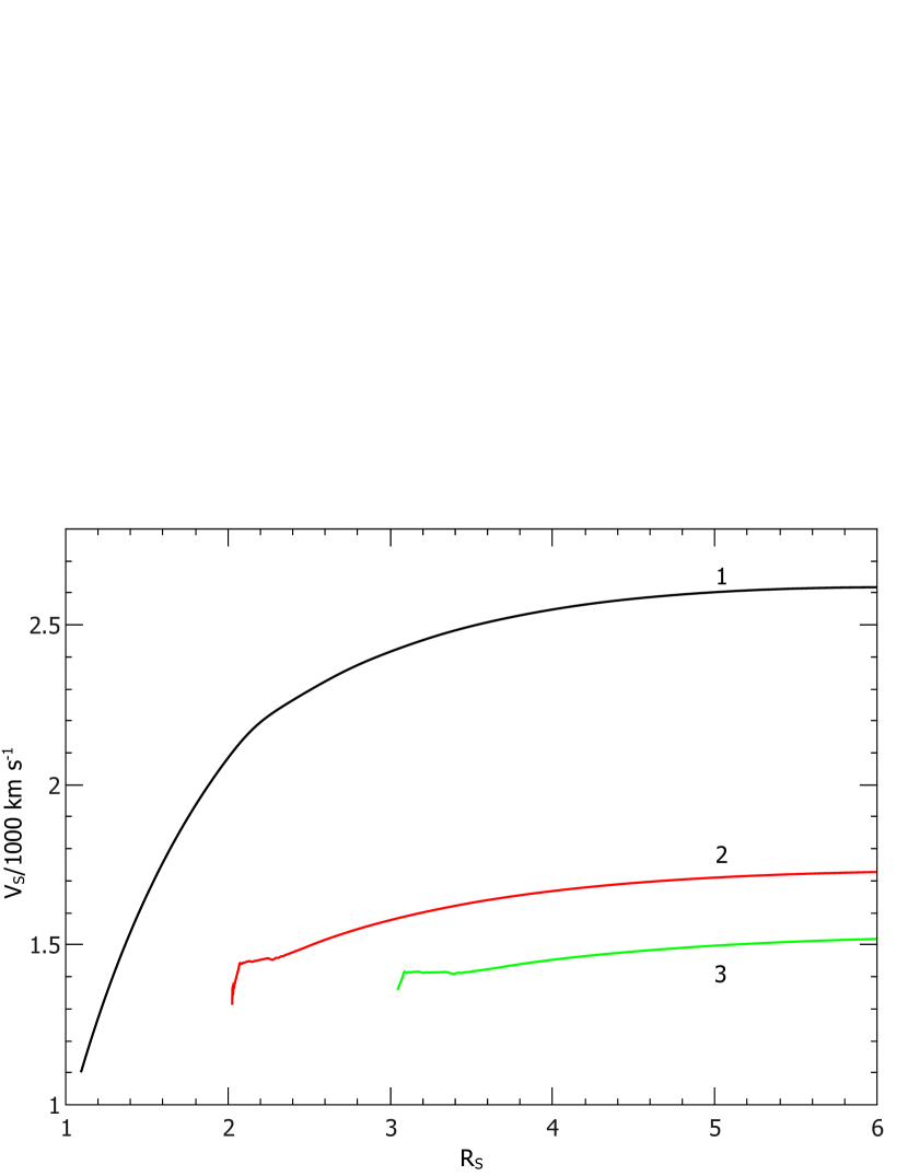
Figure 1.— Shock speed ${V_{s}}$ as a function of its radius ${R_{s}}$ for various initial CME radii ${R_{p0}}$. Curves 1, 2, and 3 correspond to ${R_{p0}}=$ =1, 2, 3, respectively. The CME speed (${V_{p}}$) is constant and equals 1000 km s^-1.

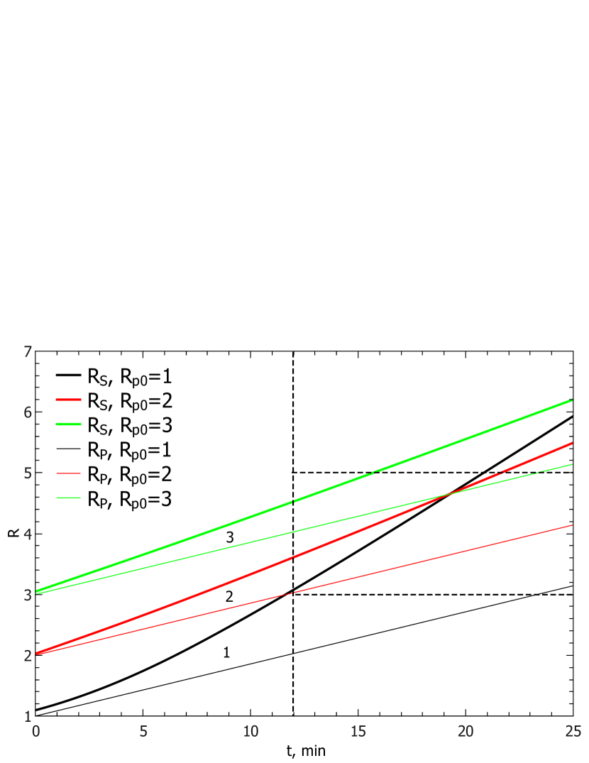
Figure 2.— Radii of shock fronts (thick lines) and CME (thin lines) as functions of time for three initial CME radii. ${V_{p}}=1000$ km s^-1. Curves 1, 2, and 3 correspond to ${R_{p0}}=$ =1, 2, 3, respectively.

The energy spectrum over frequency in the range $\nu_{1}\leq\nu\leq\nu_{0}$ may be expressed as (Suzuki & Inutsuka, 2006)

$${E_{\nu}}={E_{v0}}{\left({\nu/{\nu_{0}}}\right)^{-\beta}}{\left({r/{R_{\odot}}}\right)^{-\delta}},$$ (5)

where $\beta=1$, ${\nu_{1}}=10^{-3}$ Hz, and $\nu_{0}=5\times 10^{-2}$ Hz. It is expected that for $\nu>{\nu_{0}}$ the spectrum will be softer. In the calculations, we use Kolmogorov’s power-law index $\beta=5/3$, the same as in the inertial part of the spectrum in interplanetary space (Tu & Marsch, 1995). The ratio $\nu=k(w+\delta_{\nu}c_{a})/(2\pi)$ and the condition of particle resonance scattering $k=\rho_{B}^{-1}$ results in $\nu/{\nu_{0}}=\left({{p_{0}}/p}\right)(B/B_{\odot})(w+{\delta_{w}}{c_{a}})/{c_{a\odot}}$, where ${p_{0}}/{m_{p}}c=e{B_{\odot}}{c_{a\odot}}/(2\pi{\nu_{0}}{m_{p}}{c^{2}})$, and ${\delta_{\nu}}=(E_{\nu}^{+}-E_{\nu}^{-})/E_{\nu}$. We determine the diffusion coefficient from the spatial energy density of waves with $\nu\geq\nu_{0}$, which provides the particle scatterings: ${E_{w}}(\nu\geq\nu_{0})=E_{w\odot}/[1+(\beta-1)\ln(\nu_{0}/\nu_{1})]$ and ${\nu_{0}}{E_{\nu 0}}=(\beta-1)E_{w}(\nu\geq\nu_{0})$. Here $E_{w\odot}=E_{w}(\nu\geq\nu_{1})$ is the total energy density, which can be found from the ratio ${E_{w\odot}}={F_{\odot}}/{c_{a\odot}}$, where ${F_{\odot}}$ is the energy flow density of waves moving from the Sun, and ${w_{\odot}}\ll{c_{a\odot}}$ is used. In the calculation, we use ${F_{\odot}}\simeq 5\times{10^{5}}$ erg cm^-2s^-1) (Berezhko & Taneev, 2013, and references therein). Hence, we get the expression for the particle diffusion coefficient

$$\kappa={\kappa_{p}}{\kappa_{r}},$$ (6)

where

$${\kappa_{p}}={\kappa_{0}}\frac{{{{\left({p/{m_{p}}c}\right)}^{3-\beta}}}}{{\sqrt{1+{{\left({p/({m_{p}}c)}\right)}^{2}}}}},$$

$${\kappa_{r}}={\left({r/{R_{\odot}}}\right)^{\delta-4\beta+2}}{\left({\frac{{{w_{\odot}}/{c_{a\odot}}+{\delta_{\nu}}n_{1}^{0.5}}}{{{n_{1}}}}}\right)^{\beta-1}},$$

${\kappa_{0}}={m_{p}}{c^{3}}{B_{\odot}}{\left({{p_{0}}/({m_{p}}c)}\right)^{\beta-1}}/\left({32{\pi^{2}}e{\nu_{0}}{E_{\nu 0}}}\right)$, $E_{w}(\nu\geq\nu_{0})=4.35\times 10^{-3}$ erg cm^-3, and ${n_{1}}=n/{n_{\odot}}$.

In our calculation, we take into account the particle diffusion along the magnetic field only, and, as mentioned above, we assume that $\kappa\equiv\kappa_{\parallel}$ . Particle diffusion across the magnetic field is not considered because according to the results of the two-component (2D-slab) turbulence theory in the inner heliosphere, $\kappa_{\perp}\ll\kappa_{\parallel}$ (Zank et al., 2004).

SEP spectra generation in the solar corona mainly depends on the diffusion coefficient. The properties of the Alfven turbulence spectrum used are, in fact, free parameters. They can be determined from the comparison of the model calculations to the observation results of SEPs. The dependences of the diffusion coefficient on energy for $\beta=5/3$ and on radius for various $\beta$ and $\delta$ are shown in Figures 3 and 4, respectively.

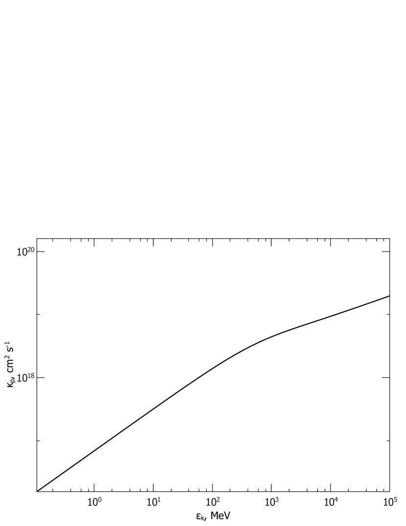
Figure 3.— Dependence of the diffusion coefficient on energy for $\beta=5/3$.

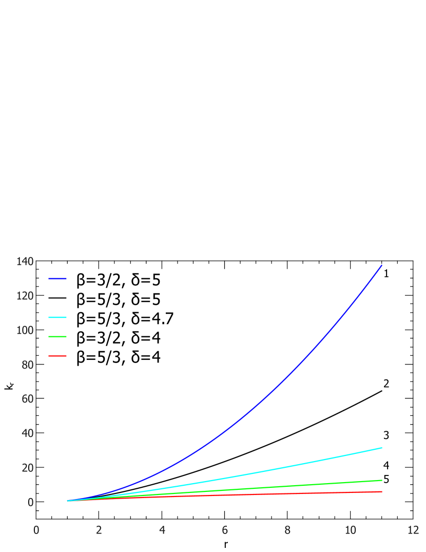
Figure 4.— Dependence of the diffusion coefficient on radius for various $\beta$ and $\delta$. Curve 1 is for $\beta=3/2$ and $\delta=5$, curve 2 is for $\beta=5/3$ and $\delta=5$, curve 3 is for $\beta=5/3$ and $\delta=4.7$, curve 4 is for $\beta=3/2$ and $\delta=4$, and curve 5 is for $\beta=5/3$, $\delta=4$.

4. Results and discussion

The formulated problem, Equations (1)–(6) with edge conditions of $f\left({r\to\infty,p,t}\right)=0$, and ${\left({\partial f/\partial r}\right)_{|{R_{p}}}}=0$ has been solved numerically. The solution algorithm for the particle transport equation is similar to the one developed by Berezhko et al. (1996) to describe cosmic-ray acceleration in supernova remnants. For the Alfven wave distribution with direction, we adopt $E_{\nu}^{+}/{E_{\nu}}=0.7$, $E_{\nu}^{-}/{E_{\nu}}=0.3$ and thus ${\delta_{\nu}}=0.4$ in all calculation cases. Figure 5 shows the accelerated particle intensity of $J\left({{\varepsilon_{k}}}\right)={p^{2}}{f_{p}}$ at the shock front, which depends on the kinetic energy, for three shock front radii of ${R_{s}}=4,5,6$ with the following parameters: $\beta=5/3$, $\delta=5$, ${\kappa_{1}}={\kappa_{p}}{\kappa_{r}}$, ${\kappa_{2}}={\kappa_{p}}$, ${V_{p}}=1000$ km s^-1, and ${R_{p0}}=3$. We assume that the above parameters are standard and will only mention if they differ in the sequel. In the energy range of ${\varepsilon_{\rm inj}}\leq{\varepsilon_{k}}\leq{\varepsilon_{m}}\left(t\right)$, a region of power-law spectrum is formed, the index of which corresponds to the stationary spectrum of ${q_{J}}=\left({{q_{f}}-2}\right)/2\approx 1.25$, where ${q_{f}}=3{\sigma_{\rm ef}}/\left({{\sigma_{\rm ef}}-1}\right)=4.5$ is the power-law index of the particle spectrum accelerated by the plane shock front with ${\sigma_{\rm ef}}=u^{\prime}_{1}/u^{\prime}_{2}=3$. The characteristic value of ${\varepsilon_{m}}(t)$ limiting the power-law spectrum region is equal to the energy of particles whose time of cyclic movement in the vicinity of the shock front equals to the average time $t_{k}$ defined in the Appendix, Equation A4. The value of ${\varepsilon_{m}}\left(t\right)$, indicated in Figure 5 by downward arrows, changes in time, as in the acceleration by the plane shock front. The value of ${\varepsilon_{m}}\left(t\right)={\varepsilon_{\rm inj}}{\left({{p_{m}}/{p_{\rm inj}}}\right)^{2}}$ is defined by Equation (A9), in the Appendix.

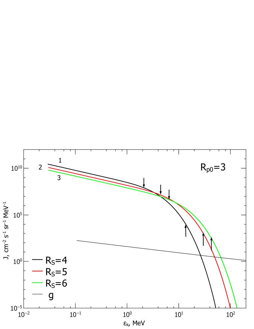
Figure 5.— Particle intensity at the shock front as a function of kinetic energy for three shock radii of ${R_{s}}=$ 4, 5, 6, they are denoted by digits 1, 2, and 3, respectively. The initial CME radius is $3{R_{\odot}}$. The $\downarrow$ synbols mark the values of ${\varepsilon_{m}}(t)$ limiting the power-law spectrum region. The $\uparrow$ symbols mark the values of ${\varepsilon_{2}}(t)$ denoting the cutoff region width. The thin line is the modulation parameter $g$. The parameter value scale is the same as on left axis of the figure.

The decrease of the spectrum amplitude at the power-law spectrum region is caused by the spatial distribution of matter density in the solar atmosphere. The slight increase of injection energy is due to the increase of the shock speed (the lowest curve in Figure 1). The cutoff region of the spectrum adjoins to the power region. The physical reason for the cutoff formation is the dispersion of the cyclic movement time relative to the average time $t_{k}$. The spectrum shape in the cutoff region is an important parameter since high-energy SEPs form this region. The values of ${\varepsilon_{2}}\left(t\right)$ determine the width of the cutoff region and are marked by the upward arrows in Figure 5. Values of ${\varepsilon_{2}}$ are calculated according to equation (A7). As can be seen from the figure, the ratio ${\varepsilon_{2}}/{\varepsilon_{m}}$ does not depend on time. Note that the ratio of $J\left({{\varepsilon_{2}},t}\right)/J\left({{\varepsilon_{m}},t}\right)$ calculated for the plane shock front exceeds the value from our calculation is approximately 10 times. The difference is apparently due to different geometry. We calculate the particle acceleration up to ${R_{s}}=6$. Then the acceleration becomes ineffective due to a geometrical factor. The influence of the shock front size on particle acceleration is taken into account through the modulation parameter $g=R_{s}V_{s}/\kappa_{1}(R_{s},\varepsilon_{k})$. Particles with $g\leq 1$ intensively leave the vicinity of the shock front. It is the phenomenon of particle escaping which describes the injection of accelerated particles into the environment with monotonically changing parameters (Berezhko et al., 1996). The dependence of acceleration efficiency on the modulation parameter can be explained as follows: (1) the particles during cyclic movement move away from the shock front move away on a distance of the diffusive length $L\approx\kappa_{1}(R_{s},\varepsilon_{k})/V_{s}$, and (2) the acceleration efficiency depends on the ratio between $L$ and ${R_{s}}$: if $L\ll{R_{s}}$, particles return to the shock front and are accelerated; if $L\geq R_{s}$, particles may not return and their acceleration is suppressed. In Figure 5 the thin curve shows the modulation parameter for ${R_{s}}=6$. The parameter value scale is the same as on left axis of the figure.

Figure 6 presents the spatial distribution of particle intensity in relative units with ${\varepsilon_{k}}=1$ MeV for $R_{s}=$ 3.5, 4, 5, and 6. As we can see from Figure 5 the particle intensity for this energy at ${R_{s}}=4$ has almost reached the stationary value. Accordingly, its spatial distribution is similar to that of the stationary shape: the distribution is exponential ahead of the shock front, and an interval of constant value forms behind the shock front. In the subsequent expansion, the shape of the spatial distribution ahead of the shock front remains the same. The expansion of the volume filled with particles is caused by the increase of the diffusion coefficient at the shock front. The region of constant value behind the front increases with time. The left boundary of the intensity distribution behind the shock front coincides with the piston radius. The monotonic decrease of the intensity at the shock front at ${R_{s}}>4$ is caused by the decrease of the injection rate.

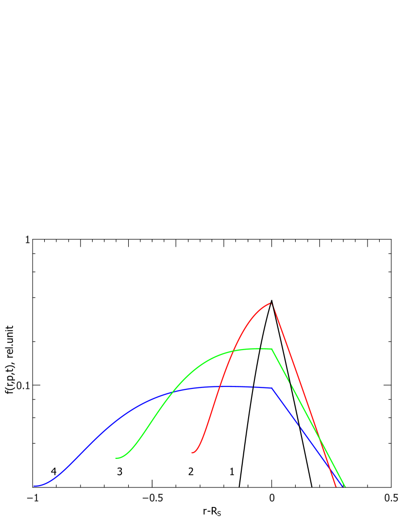
Figure 6.— Spatial distribution of particle intensity in relative units. The digits 1, 2, 3, and 4 denote the particle intensity with ${\varepsilon_{k}}=1$ MeV for four shock radii ${R_{s}}=$ 3.5, 4, 5, and 6, respectively. The left boundary of the spatial distribution behind the shock front coincides with the piston radius.

In Figure 7, the differential spectrum of the total number of accelerated particles is plotted as a function of kinetic energy, which is defined as $dN/d{\varepsilon_{k}}=(4\pi p^{2}/V)d\Omega\mathop{\smallint}_{V}f_{p}(p,r,t)r^{2}dV$, where $V$ is the volume at ${R_{s}}=6$ per the unit of a solid angle $(d\Omega=1)$. The curves in the figure correspond to the spectra of the total accelerated particle number ahead of and behind the shock front as well as their sum. The distribution depends on particle energy: there are more particles with energies of ${\varepsilon_{\rm inj}}<{\varepsilon_{k}}<3$ MeV behind the shock front, and the opposite for particles with energies of ${\varepsilon_{k}}>3$ MeV.

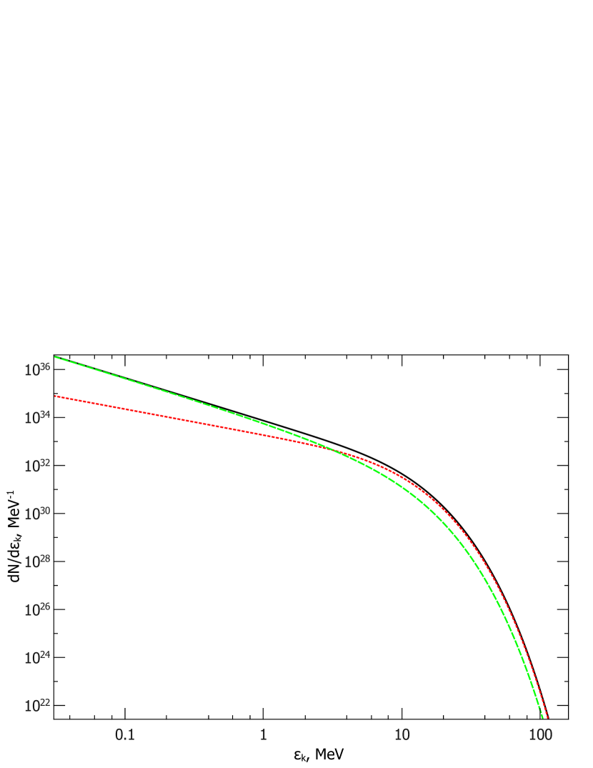
Figure 7.— Spectrum of the total accelerated particle number as a function of kinetic energy at ${R_{s}}=6$. The dashed curve represents the spectrum behind the shock front, the dotted curve represents the spectrum ahead of the shock front, and the solid curve is their sum of them and represents the spectrum of the total particle number.

Figures 8, and 9 show the particle intensities at the shock front as a function of energy for initial radii of $R_{p0}=$ 1, and 2, respectively. One can see that the smaller $R_{p0}$ is, the higher is $V_{s}$ (see Figure 1), and the more efficient is the particle acceleration. From Figures 2, 5, 8, and 9, one can conclude that the spectrum is formed 0.2–1 hr after the beginning of CME motion. At that time ${R_{p}}=$ 3 – 5 and ${R_{s}}=$ 5 – 10, and may begin an injection of particles into interplanetary medium, which is in agreement with observations.

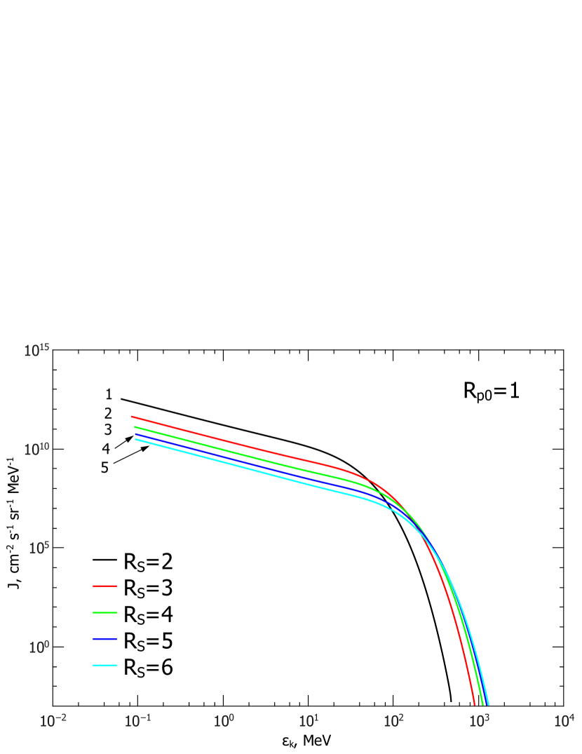
Figure 8.— Particle intensity at the shock front depending on kinetic energy for five shock radii $R_{s}=$ 2, 3, 4, 5, 6 denoted by digits 1–5, respectively. The initial CME radius is $1R_{\odot}$.

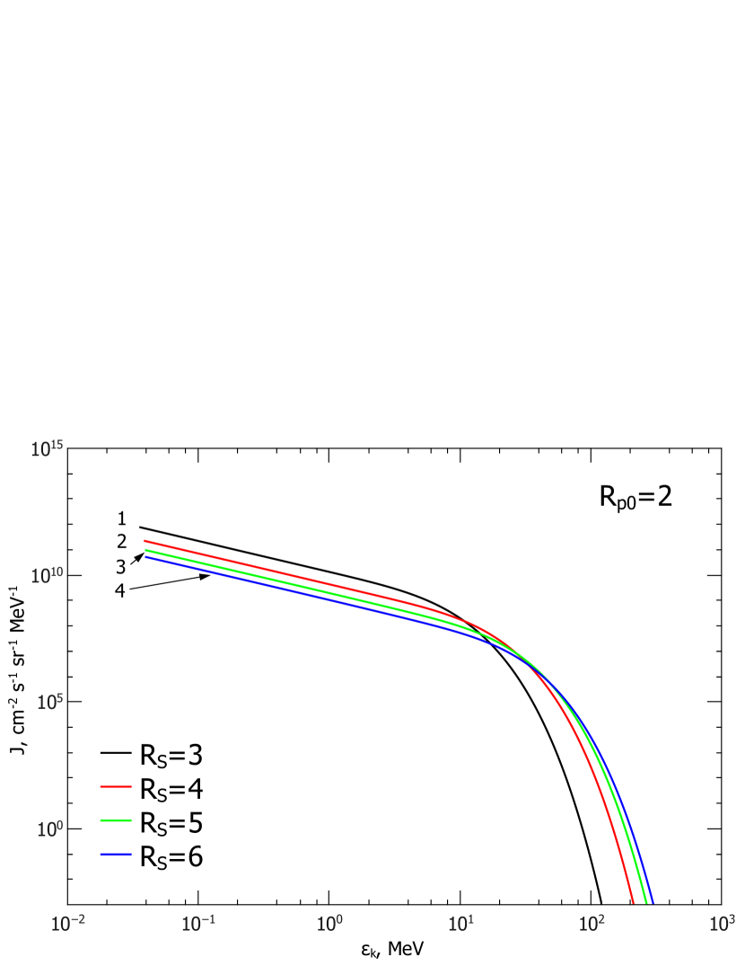
Figure 9.— Particle intensity at the shock front depending on kinetic energy for four shock radii $R_{s}=$ 3, 4, 5, 6 denoted by digits 1–4, respectively. The initial CME radius is $2R_{\odot}$.

Figure 10 shows the intensity of particles at the shock front for different values of parameters. All calculations here start at $R_{p0}=3$ and finish when ${R_{s}}=6$. The intensities marked by digit 1 in Figure 10 and digit 3 in Figure 5 are calculated with standard parameters. Curves 2–5 differ in one parameter: 2 is for $\kappa_{2}=0.1\kappa_{p}$, 3 is with $E_{w}(\nu\geq\nu_{0})=8.7\times 10^{-3}$ erg cm^-3, 4 is for $\delta=4$; and 5 is with ${V_{p}}=2000$ km s^-1. Curve 6 represents the total influence of the changes. The particle acceleration rate in the regular acceleration depends on the value of $\kappa/V_{s}^{2}$ and it can explain the intensity changes in Figure 10. Here, the parameter $\kappa$ is proportional to the sum of diffusion coefficients ahead of and behind the shock front.

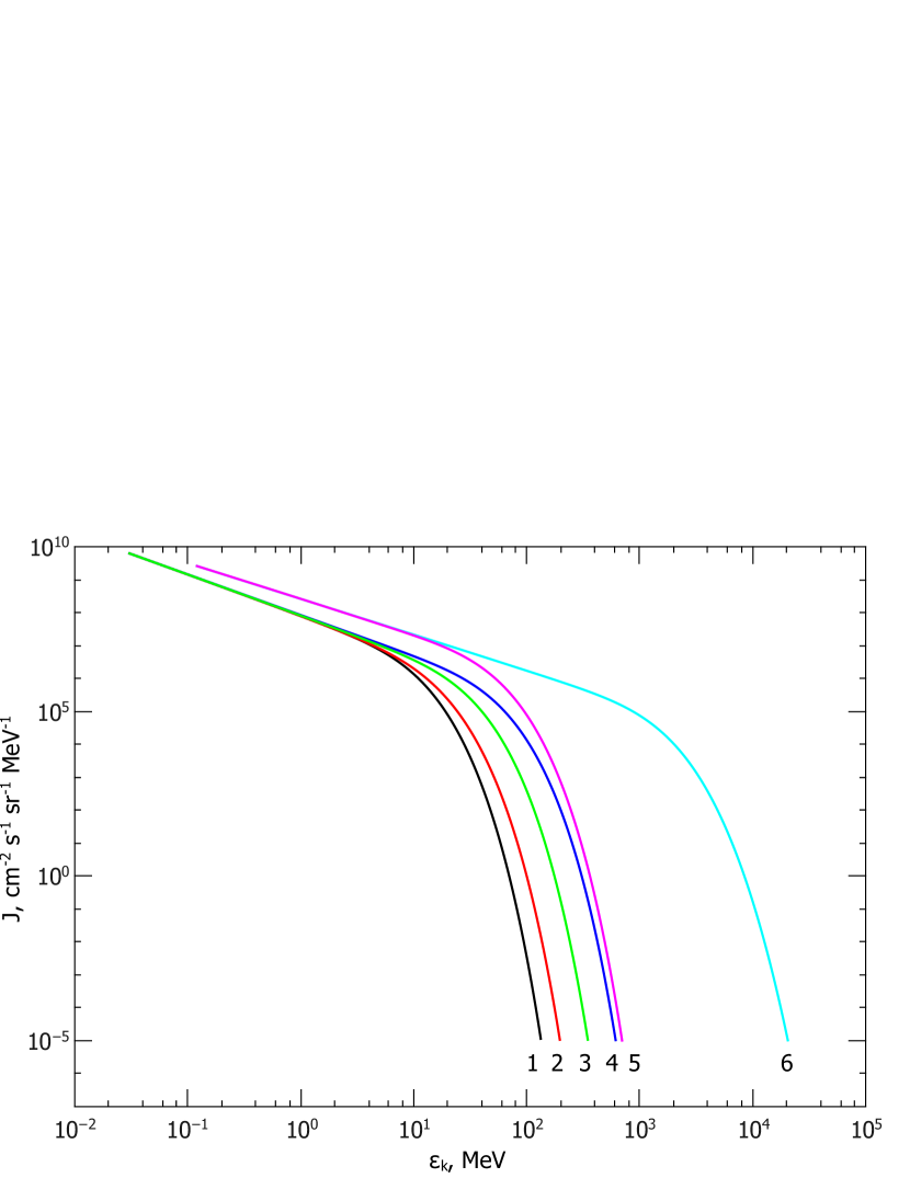
Figure 10.— Particle intensity at the shock front depending on kinetic energy for ${R_{s}}=6$ and different parameters. See the text for details.

In most cases SEP flows are measured at the Earth’s orbit. Therefore, it is necessary to somehow connect spectra of particles accelerated in the solar atmosphere and ones registered in interplanetary space. The CME itself also influences particle propagation in interplanetary space. The extent of the influence is determined by the modulation parameter $g=R_{s}V_{s}/\kappa_{\rm ip}(R_{s},\varepsilon_{k})$, where $\kappa_{\rm ip}$ is the spatial diffusion coefficient in interplanetary space. Depending on the value of $g$ ((1) $g\gg 1$, (2) $g\sim 1$, and (3) $g\ll 1$) there are three possible scenarios for particle propagation. In the first case, the CME influences the form of the spectrum and particle spatial distribution. In observations, the first case describes ESPs (particles with $\varepsilon_{k}\leq 10$ MeV the flow of which after a plateau reaches a maximum at the shock front). In the second case, the CME only influences the particle spatial distribution. The second scenario describes particles with $10<\varepsilon_{k}<50$ MeV nucleon^-1 in observations and their constant flow value retains to CME arrival (Reames, 1990). In the third case, the CME does not affect particle propagation. In observations, these SEPs are particles with ${\varepsilon_{k}}\geq 100$ MeV nucleon^-1. A “black box” model (Kallenrode & Wibberenz, 1997) is widely used in order to determine SEP flows in gradual events. The particle distribution in interplanetary space from the source can be obtained from the model; the source is assigned a particle spectrum at the moving shock front (Heras et al., 1992, 1995; Kallenrode & Wibberenz, 1997; Lario et al., 1998; Kallenrode & Hatzky, 1999). The model does not take into account the correlation of particle flow characteristics with the phenomena occurring at the shock front. Detailed dynamic and self-consistent models of the shock propagation and particle acceleration have been developed by Zank et al. (2000) for strong shock waves and by Rice et al. (2003) for shock waves with arbitrary intensities. Using these models, Li et al. (2003) have invented a numerical method known as Particle Acceleration and Transport in the Heliosphere (PATH) to simulate SEP events in interplanetary space. The model includes local particle injection at the moving quasi-parallel shock wave, diffusive shock acceleration, self-consistent Alfven wave generation by accelerated particles, particle trapping and escape from the complex shock, and particle propagation in the inner heliosphere. Using the PATH method, the characteristics of heavy nucleus flow (Li et al., 2005; Zank & Verkhoglyadova, 2007), and the dependence of particle flow characteristics on the angle between the magnetic field and the normal to the shock front, including heavy nucleus (Li et al., 2009, 2012), have been calculated. The diffusion coefficient used was determined from the two-component (2D-slab) turbulence theory (Zank et al., 2004, 2006). The distribution depends on particle energy. The comparison of the calculated results with specific events (Verkhoglyadova et al., 2009, 2012), including a mixed population of both flare and shock-accelerated particles (Verkhoglyadova et al., 2010), shows their general agreement. The agreement demonstrates that the PATH model takes into account the main physical factors determining SEP acceleration and propagation. In this paper, we will consider the third scenario only. The simplified approach of particle propagation is formulated following Berezhko & Taneev (2003). Particle propagation is described by the transport equation for the distribution function of $f(r,p,t)$ in diffusive approximation:

$$\frac{{\partial f}}{{\partial t}}=\frac{1}{{{r^{2}}}}\frac{\partial}{{\partial r}}\left({\kappa{r^{2}}\frac{{\partial f}}{{\partial r}}}\right)+Q,$$

where $Q=F(p)/(\Omega_{s}R_{f}^{2})\delta(t-t_{f})$ is the source term and $F(p)/\Omega_{s}$ is the spectrum of the total particle number accelerated in the solar atmosphere per unit solid angle. The source term shows that the particles accelerated by the time ${t_{f}}$ occupy a volume with radius ${R_{f}}$ and will instantly be injected into the surrounding medium when $t={t_{f}}$. The solution of the equation at $r\gg{R_{f}}$ and $t>{t_{f}}$ is as follows (Krimigis, 1965):

$$f\left({r,p,t}\right)=\frac{{F\left(p\right)}}{{2{{{\Omega}}_{s}}r_{e}^{3}}}\frac{1}{{t_{*}^{3}}}{e^{-{r_{*}}/{t_{*}}}},$$

where $t_{*}=t/T$, ${r_{*}}=r/{r_{e}}$, and $T=r_{e}^{3}/\kappa_{\rm ip,e}$. In the calculations, the expression $\kappa\propto r$ (Berezhko & Taneev, 2003) is used. The maximum of the distribution function at ${r_{*}}=1$ occurs at $t_{*,\rm max}=1/3$. As a result, we can derive the spectrum of maximal intensities as a function of kinetic energy:

$$J_{\rm max}={p^{2}}f\left({{r_{*}}=1,p,{t_{*,max}}}\right)=0.67\frac{{{p^{2}}F\left(p\right)}}{{{{\Omega}_{s}}r_{e}^{3}}}.$$ (7)

Figure 11 shows the intensity of the maximum values in depending on the kinetic energy at the Earth’s orbit, according to Equation (7). For the injected particles, we use the spectra of the total number of particles at ${R_{s}}=6$ for the three variants shown in Figures 5, 8, and 9. One can see from Figure 11 that the smaller $R_{p0}$ is, and accordingly the higher $V_{s}$ is, the higher are the particles’ flux and maximum energies.

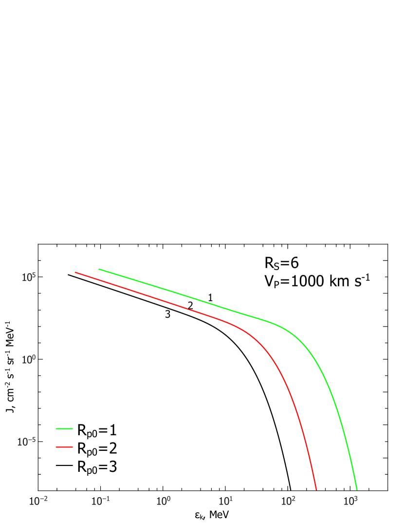
Figure 11.— Intensity of the maximum values of particles’ flux depending on kinetic energy at the Earth’s orbit. Curves marked by digits 1, 2, and 3 correspond to CME radii $R_{p0}=$ 1, 2, and 3, respectively.

Figure 12 presents the SEP intensity depending on the energy at the Earth’s orbit for three GLE events (Bombardieri et al., 2007; Krymsky et al., 2015). As we know from observations, ${V_{p}}=1200$ km s^-1 and ${R_{p0}}=1.5$ for the event on 2001 April 15 (Bombardieri et al., 2007). We use the following values in the calculation: $\delta=4$, ${\kappa_{1}}={\kappa_{p}}{\kappa_{r}}$, ${\kappa_{2}}={\kappa_{p}}$, and ${V_{p}}=1200$ km s^-1. The process starts from $R_{p0}=1.5$ and terminates when ${R_{s}}=6$. We use $\beta=5/3$ and ${E_{w}}\left({\nu\geq{\nu_{0}}}\right)=8.7\times 10^{-3}$ erg cm^-3 to calculate curve 1, shown in Figure 12. Apparently, the maximal energy in the spectrum agrees with the observations; however, the cutoff shape significantly differs from the registered one.

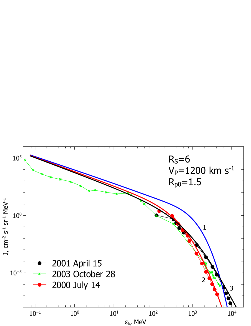
Figure 12.— Intensity of the maximal values of the SEP flux as a function of kinetic energy at the Earth’s orbit. The following symbols denote measurements: asterisks are from 2003 October 28 (Krymsky et al., 2015), red circles are from 2000 July 14, and black circles are from 2001 April 15 (Bombardieri et al., 2007). Calculation curves correspond to the following parameters: (1) $\beta=5/3$, $E_{w}(\nu\geq\nu_{0})=8.7\times 10^{-3}$ erg cm^-3; (2) $\beta=2.2$, $E_{w}(\nu\geq\nu_{0})=3.05\times 10^{-2}$ erg cm^-3; and (3) $\beta=2.4$, $E_{w}(\nu\geq\nu_{0})=1.1\times 10^{-1}$ erg cm^-3.

The shape of the spectrum near cutoff energies is determined by the dependence of the diffusion coefficient on energy. According to equation (6), $\kappa_{p}\propto[p/(m_{p}c)]^{2-\beta}$ for relativistic energies; therefore, the diffusion coefficient decreases with the increase of particle energy if $\beta>2$. However, the increase of the wave spectrum power index causes the increase of the diffusion coefficient at low energies and suppresses acceleration efficiency. Thus, the increase of $\beta$ requires the increase of $E_{w}(\nu\geq\nu_{0})$. Curves 2 and 3 in Figure 12 are calculated with $\beta=2.2$, $E_{w}(\nu\geq\nu_{0})=3.05\times 10^{-2}$ erg cm^-3 and $\beta=2.4$, $E_{w}(\nu\geq\nu_{0})=1.1\times 10^{-1}$ erg cm^-3, respectively. One can see that in these cases, the calculated spectra agree with the registered ones. However, the assumed values of $E_{w}(\nu\geq\nu_{0})$ significantly exceed the standard values. We can suggest some possible reasons for the agreement with the standard values: (1) the values of $\nu_{1}$, and $\nu_{0}$ in the solar atmosphere are an order of magnitude greater than the used ones; (2) the wave spectrum in the inertial region has a more complicated dependence on frequency—for example, it consists of two parts with different power-law indexes; and (3) the wave energy increases due to the generation by accelerated particles. We do not discuss here the difference between the calculated and measured spectra at low energies $\varepsilon_{k}<100$ MeV because the Krimigis model does not describe the interplanetary propagation of particles with such energies.

5. Conclusion

The relationship between the CME and the shock speeds moving in the solar atmosphere is defined from the solution of the gas-dynamic equations. The shock speed increases with the decrease of the initial CME radius. The accelerated particle spectra as a function of time has been reproduced by numerical solution of the diffusive transport equation with a set of realistic parameters. Depending on the initial CME radius, its speed, and Alfven wave magnetic energy for $\beta=5/3$, the accelerated particle spectrum is established at 10 – 60 minutes after the beginning of CME motion. The maximum energies of the particles reach 0.1–10 GeV. By that time, the CME radii are 3 – 5 $R_{\odot}$ and the shock front radii are 5 – 10 ${R_{\odot}}$, which agree with observations. The calculation results and observations are in agreement if $\beta>2$. However, in this case the Alfven wave magnetic energy is significantly higher than the standard one.

Appendix A Particle Acceleration by Plane Shock Front

To estimate the accuracy of the numerical algorithm, we calculate the particle acceleration by the plane shock front, which has a constant speed ${V_{s}}$ and moves in infinite medium. The corresponding particle transport equation for an isotropic distribution function $f_{i}(x,p,t)$ is

$$\frac{{\partial{f_{i}}}}{{\partial t}}={\kappa_{i}}\frac{{{\partial^{2}}{f_{i}}}}{{\partial{x^{2}}}}-{w_{i}}\frac{{\partial{f_{i}}}}{{\partial x}}+\frac{{{N_{0}}{u_{1}}}}{{4\pi p_{\rm inj}^{2}}}\delta\left({p-{p_{\rm inj}}}\right)\delta\left({x-{x_{s}}}\right)H\left(t\right),$$

where the subscript $i$ can be 1 or 2, corresponding to the regions ahead of $(x>{x_{s}})$ and behind $(x<{x_{s}})$ the shock front, respectively; $\kappa_{1}$ and $\kappa_{2}$ are the spatial diffusion coefficients; $w_{1}$ and ${w_{2}}=\left({\left({\sigma-1}\right){V_{s}}+{w_{1}}}\right)/\sigma$ are the flow velocity ahead of and behind the shock front; $\sigma$ is the compression ratio; ${x_{s}}={x_{s0}}+{V_{s}}t$ is the front position; ${u_{1}}={V_{s}}-{w_{1}}$; ${N_{0}}$ is the particle number density injecting at the momentum $p_{\rm inj}$; and $H$ is the Heaviside function. In the case when the coefficients $\kappa_{1}$ and $\kappa_{2}$ are constants and relate to each other as $\kappa_{1}/\kappa_{2}=\sigma^{2}$, the task has an exact solution:

$${f_{1}}/{f_{\infty}}=0.5{\rm erfc}\left({\sqrt{\frac{{{t_{0}}}}{t}}\left({a1+a3}\right)/4-\sqrt{\frac{{{t_{0}}}}{t}}}\right)+0.5{\left({\frac{p}{{{p_{\rm inj}}}}}\right)^{a3}}{\rm erfc}\left({\sqrt{\frac{{{t_{0}}}}{t}}\left({a1+a3}\right)/4+\sqrt{\frac{{{t_{0}}}}{t}}}\right),$$ (A1)

$${f_{2}}/{f_{\infty}}=0.5{\rm erfc}\left({\sqrt{\frac{{{t_{0}}}}{t}}\left({a2+a3}\right)/4-\sqrt{\frac{{{t_{0}}}}{t}}}\right)+0.5{\left({\frac{p}{{{p_{\rm inj}}}}}\right)^{a3}}{e^{a2}}{\rm erfc}\left({\sqrt{\frac{{{t_{0}}}}{t}}\left({a2+a3}\right)/4+\sqrt{\frac{{{t_{0}}}}{t}}}\right),$$

where ${f_{i}}\left({x,p,t}\right)/{f_{\infty}}$ is the relative spectrum; ${f_{\infty}}=f\left({{p_{\rm inj}}}\right){\left({p/{p_{\rm inj}}}\right)^{-q}}$, with $q=3\sigma/\left({\sigma-1}\right)$, is the stationary spectrum of accelerated particles at the shock front; ${t_{0}}=4{\kappa_{1}}/u_{1}^{2}$; ${u_{2}}={u_{1}}/\sigma$; ${a_{1}}={u_{1}}\left({x-{x_{s}}}\right)/{\kappa_{1}}$; ${a_{2}}={u_{2}}\left({{x_{s}}-x}\right)/{\kappa_{2}}$; ${a_{3}}=3\left({\sigma+1}\right)/\left({\sigma-1}\right)\ln\left({p/{p_{\rm inj}}}\right)$; and ${\rm erfc}$ is the additional probability integral. To derive the above expressions, the Laplace transformation in time is used.

The solution (A1) at the shock front $x=x_{s}$ is similar to that obtained in Berezhko et al. (1988) and Axford (1981). Figure 13 presents the relative spectrum of accelerated particles at the shock front ${f={f_{1}}\left({{x_{s}},p,t}\right)/{f_{\infty}}}$ as a function of momentum for five successive time instants. Figure 14 shows the spatial distribution of the relative particle spectrum ($f=f_{1}(x>x_{s},p_{*},t)/f_{\infty}$, $f=f_{2}(x<x_{s},p_{*},t)/f_{\infty}$) whose momentum logarithm is 1 ($\ln\left({{p_{*}}/{p_{\rm inj}}}\right)=1$) as a function of distance for five successive time moments. The deviations of the corresponding values of the numerical solution from the exact solution in percent are given at the top panels of the figures.

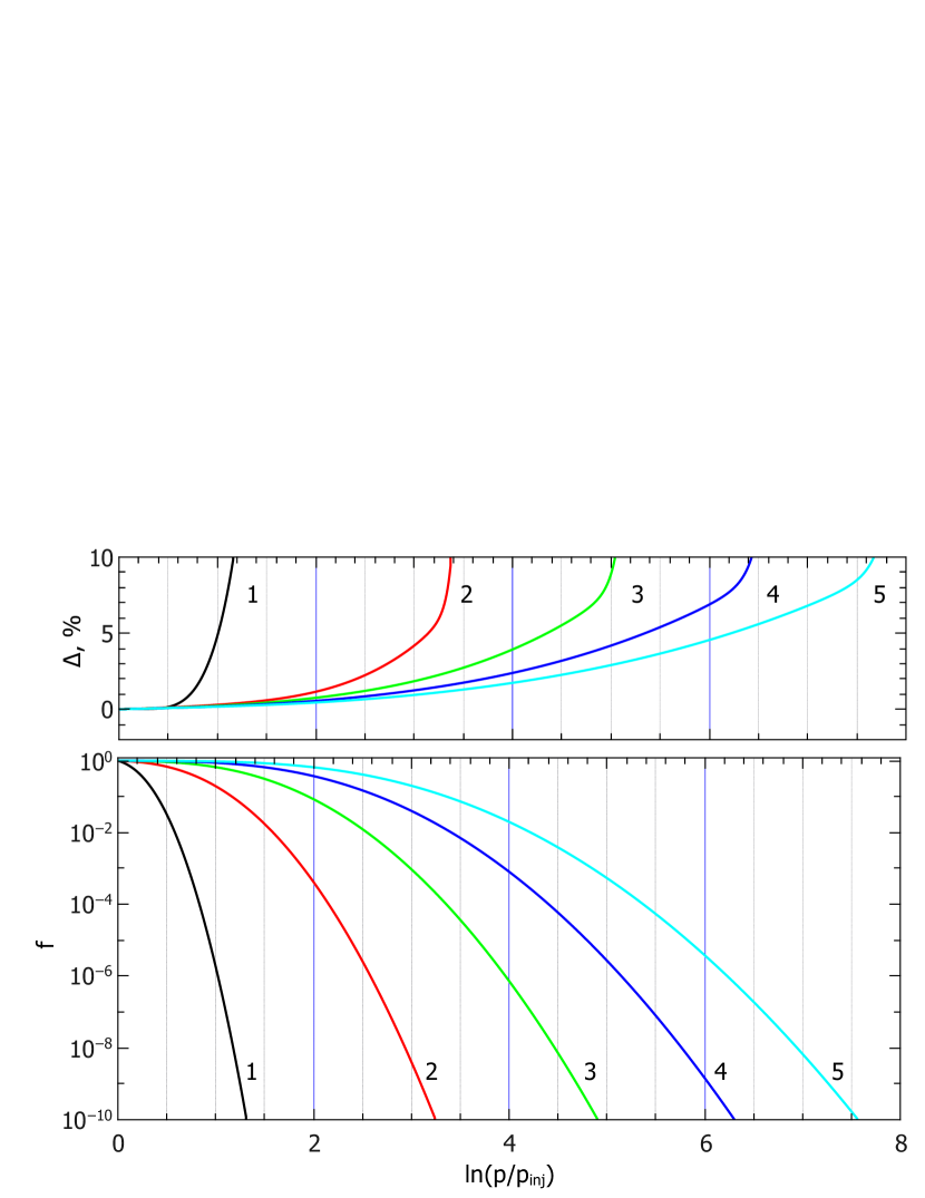
Figure 13.— Particle spectrum at the shock front as a function of momentum for five successive time moments. $f=f_{1}(x_{s},p_{*},t)/f_{\infty}$ is the relative particle spectrum and ${f_{\infty}}$ is the stationary spectrum. On the top panel, $\Delta=\left({f-{f_{\rm ex}}}\right)/{f_{\rm ex}}\times 100\%$ is the deviation of the relative spectrum of the numerical solution from the exact solution in percent; ${f_{ex}}$ is the relative spectrum of the exact solution.

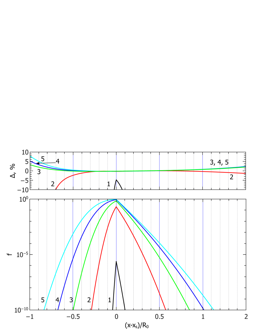
Figure 14.— Spatial distribution of the particle spectrum for five successive time moments. $f=f_{1}(x>x_{s},p_{*},t)/f_{\infty}$, $f=f_{2}(x<x_{s},p_{*},t)/f_{\infty}$, and $\ln(p_{*}/p_{\rm inj}=1$. On the top panel, $\Delta=\left({f-{f_{\rm ex}}}\right)/{f_{\rm ex}}\times 100\%$ is the deviation of the spatial spectrum dependence of the numerical solution from the exact solution in percent; ${f\rm ex}$ is the spatial distribution of the relative spectrum of the exact solution.

One can see from Figures 13 and 14 that the accuracy of the calculation depends on the amplitude of the relative spectrum. The relative deviation does not exceed a few percent if the value is higher than $10^{-6}$. In general, the comparison confirms the sufficient accuracy of the numerical calculation algorithm.

The exact solution (A1) describes the formation of the accelerated particle spectrum in time. The shape of the spectrum depends on the momentum. The shape is mainly determined by the first term in equation (A1). The value of ${p_{m}}\left(t\right)$, which separates different shapes of the spectrum, can be found from (A1) by equating the argument of the first additional probability integral to zero. Hence, following this equation,

$$f\left({{x_{s}},{p_{m}},t}\right)/{f_{\infty}}\left({{p_{m}}}\right)\approx 0.5$$

and

$$\frac{p_{m}(t)}{p_{\rm inj}}={\text{exp}}\left[{\frac{{\left({\sigma-1}\right)}}{{3\left({\sigma+1}\right)}}\frac{{u_{1}^{2}t}}{\kappa_{1}}}\right].$$ (A2)

The value of ${p_{m}}\left(t\right)$ separates the momentum region of ${p_{inj}}\leq p\leq{p_{m}}\left(t\right)$, where the spectrum is close to a stationary one, and the region $p>{p_{m}}\left(t\right)$, where the greater the momentum, the more the spectrum deviates from the stationary one. The width of the cutoff region can be determined by equating the argument of the first term in Equation A1 to the value of A;

$$\sqrt{\frac{{{t_{0}}}}{t}}\frac{3}{4}\frac{{\left({\sigma+1}\right)}}{{\left({\sigma-1}\right)}}\ln\frac{{{p_{2}}}}{{{p_{\rm inj}}}}-\sqrt{\frac{{{t_{0}}}}{t}}=A,$$

and therefore

$$\frac{{{p_{2}}}}{{{p_{m}}}}={\text{exp}}\left[{A\sqrt{\frac{{4\left({\sigma+1}\right)}}{{3\left({\sigma-1}\right)}}\ln\frac{{{p_{m}}}}{{{p_{\rm inj}}}}}}\right],$$ (A3)

where Equation A2 is used. Here $A$ defines the deviation value of the spectrum from the stationary one $f\left({{p_{2}},t}\right)/{f_{\infty}}\left({{p_{2}}}\right)\approx{\rm erfc}\left(A\right)$ at momentum ${p_{2}}$. The width of the cutoff region increases with time. The temporary dynamics of the spatial distribution, shown in Figure 14, is the same for all momenta, differing by the offset. Figures 13 and 14 show that the spatial distribution in the region ahead of the shock front becomes exponential, with an interval of constant value being formed in the region behind the shock front. The subsequent changes in the spatial distribution are only an expansion of the interval.

Let us consider the approximate solution of the problem of particle acceleration by the plane shock front when the diffusion coefficients depend on momentum. Such a solution can be used to interpret the particle spectrum dependence on task parameters.

It is known that the acceleration of particles by the regular mechanism is caused by the cyclic particle movement in the vicinity of the shock front (Krymsky, 1977; Bell, 1978). Statistical characteristics of the movement, such as the average time of ${t_{k}}$ that particles spend on $k$ cycles, and the corresponding dispersion is $d_{k}^{2}$, are as follows (Forman & Drury, 1983; Berezhko et al., 1988):

$$t_{k}=\frac{3}{{{u_{1}}-{u_{2}}}}\int_{p_{\rm inj}}^{p_{k}}\left({{\kappa_{1}}/{u_{1}}+{\kappa_{2}}/{u_{2}}}\right)\frac{{dp}}{p},\,\,\,\,d_{k}^{2}=6/\left({{u_{1}}-{u_{2}}}\right)\int_{p_{\rm inj}}^{p_{k}}\left({\kappa_{1}^{2}/u_{1}^{3}+\kappa_{2}^{2}/u_{2}^{3}}\right)\frac{{dp}}{p}.$$ (A4)

From the comparison of ${t_{k}}$ from equation (A4) for ${\kappa_{1}}/{\kappa_{2}}={\sigma^{2}}$ with its counterpart from Equation (A2), we get ${t_{k}}=t$ and ${p_{k}}={p_{m}}$. Hence, the characteristic value of ${p_{m}}\left(t\right)$ is equal to the particle momentum, the time of a cyclic movement which is equal to the average time $t_{k}$.

Using the central limit theorem of probability theory and ${t_{k}}$, $d_{k}^{2}$, one can find the particles’ distribution function (Berezhko et al., 1988):

$$\frac{f}{{{f}_{\infty}}}=0.5~{}{\rm erfc}\left(\sqrt{\frac{{{\delta}_{1}}{{t}_{k}}}{t}}-\sqrt{\frac{{{\delta}_{1}}t}{{{t}_{k}}}}\right)+0.5{{e}^{4{{\delta}_{1}}}}~{}{\rm erfc}\left(\sqrt{\frac{{{\delta}_{1}}{{t}_{k}}}{t}}-\sqrt{\frac{{{\delta}_{1}}t}{{{t}_{k}}}}\right),$$ (A5)

where ${{\delta}_{1}}=t_{k}^{2}/2d_{k}^{2}$. If in the approximate solution $\kappa_{1}/\kappa_{2}=\sigma^{2}$, then the solution from Equation (A5) according to Equation (A4) is the same as that for Equation (A1). If ${{\kappa}_{1}}={{\kappa}_{10}}{{\left(p/{{p}_{\rm inj}}\right)}^{\alpha}}$, ${{\kappa}_{2}}={{\kappa}_{20}}{{\left(p/{{p}_{inj}}\right)}^{\alpha}}$, and ${{\left(p/{{p}_{inj}}\right)}^{\alpha}}\gg 1$, it follows from Equation (A4) that

$${{t}_{k}}=\frac{{{\kappa}_{10}}}{u_{1}^{2}}\frac{q}{\alpha}\left(1+\sigma\frac{{{\kappa}_{20}}}{{{\kappa}_{10}}}\right){{\left(\frac{{{p}_{k}}}{{{p}_{\rm inj}}}\right)}^{\alpha}},\,\,\,\,d_{k}^{2}={{\left(\frac{{{\kappa}_{10}}}{u_{1}^{2}}\right)}^{2}}\frac{q}{\alpha}\left(1+{{\sigma}^{3}}{{\left(\frac{{{\kappa}_{20}}}{{{\kappa}_{10}}}\right)}^{2}}\right){{\left(\frac{{{p}_{k}}}{{{p}_{\rm inj}}}\right)}^{2\alpha}}.$$ (A6)

The solution from equation (A5) is similar to the one from equation (A1). The values of ${p_{m}}$ and ${p_{2}}$ from equation (A5) are obtained the same way as in Equation (A1). The result is

$$\frac{{{p_{m}}}}{{{p_{\rm inj}}}}={\left({\alpha u_{1}^{2}t/\left({q{\kappa_{10}}\left({1+\sigma\frac{{{\kappa_{20}}}}{{{\kappa_{10}}}}}\right)}\right)}\right)^{1/\alpha}},\,\,\,\,\frac{{{p_{2}}}}{{{p_{m}}}}=y_{*}^{2/\alpha},\,\,\,\,\frac{{{\varepsilon_{2}}}}{{{\varepsilon_{m}}}}={\left({\frac{{{p_{2}}}}{{{p_{m}}}}}\right)^{2}},$$ (A7)

where ${{y}_{*}}=0.5B+\sqrt{1+{{\left(0.5B\right)}^{2}}}$, $B={\left[2\alpha\left(1+{{\sigma}^{3}}{{\left({{\kappa}_{20}}/{{\kappa}_{10}}\right)}^{2}}\right)/(q{{\left(1+\sigma{{\kappa}_{20}}/{{\kappa}_{10}}\right)}^{2}}\right]^{0.5}}A$.

In the case of spatial dependence of the diffusion coefficients on radius, we can generalize expression (A7). Taking into account the definition of $p_{m}(t)$, it is possible to write the equation

$$\frac{d{{p}_{m}}}{dt}=\frac{\Delta p}{\langle t\rangle}={{p}_{m}}\frac{\left({{u}_{1}}-{{u}_{2}}\right)}{3\left({{\kappa}_{1}}/{{u}_{1}}+{{\kappa}_{2}}/{{u}_{2}}\right)},$$ (A8)

where $\langle t\rangle=4({{\kappa_{1}}/{u_{1}}+{\kappa_{2}}/{u_{2}}})/v$ is the average time of one cycle of a particle; $\Delta{p_{m}}=4{p_{m}}\left({{u_{1}}-{u_{2}}}\right)/3v$ is the average momentum change of a particle over one cycle; and $v$ is the particle speed (Berezhko et al., 1988). For the exact solution $\left({{\kappa_{1}}/{\kappa_{2}}={\sigma^{2}}}\right)$ with diffusion coefficients depending on the momentum of $(\kappa\propto p^{\alpha})$, after integrating equation (A8), one can obtain Eqs (A2) and (A7). We represent the parameters by ${\kappa_{1}}={\kappa_{10}}{\left({p/{p_{\rm inj}}}\right)^{\alpha}}{\left({r/{R_{0}}}\right)^{{d_{1}}}}$, ${\kappa_{2}}={\kappa_{20}}{\left({p/{p_{\rm inj}}}\right)^{\alpha}}$, where ${\kappa_{1}}$ is the diffusion coefficient ahead of the shock front, ${\kappa_{2}}$ is the counterpart behind the shock front; $R_{0}$ is the spatial scale; and ${R_{s}}={R_{S0}}{\left({t/{t_{0}}}\right)^{{d_{2}}}}$ is the shock radius depending on time. In this case the diffusion coefficient at the shock front is ${\kappa_{1}}={\kappa_{*}}{\left({p/{p_{inj}}}\right)^{\alpha}}{\left({t/{t_{0}}}\right)^{{d_{1}}{d_{2}}}}$, where ${\kappa_{*}}={\kappa_{10}}{\left({{R_{S0}}/{R_{0}}}\right)^{{d_{1}}}}$. Substituting it into equation (A8) and dividing the variables, one can obtain

$$\frac{{{p_{m}}}}{{{p_{\rm inj}}}}={\left[{\frac{{\alpha u_{1}^{2}}}{{q{\kappa_{*}}}}\mathop{\smallint}\limits_{{t_{0}}}^{t}\frac{{dt}}{{{{\left({\frac{t}{{{t_{0}}}}}\right)}^{{d_{1}}{d_{2}}}}+\alpha}}}\right]^{1/\alpha}},$$ (A9)

where ${({p_{m}}/{p_{\rm inj}})^{\alpha}}\gg 1$, $\alpha=\sigma{\kappa_{20}}/{\kappa_{*}}$. Equations (A3) and (A5) show that ${p_{2}}/{p_{m}}$ depends on ${\delta_{1}}=t_{k}^{2}/2d_{k}^{2}$, which, according to equation (A4), is determined by the ratio of the squares of the diffusion coefficients. Thus, one may assume that in this case the width of the cutoff region will still be defined by Equation (A7).

References

- Axford (1981) Axford, W.I. 1981, Proc. 17th ICRC, 12, 155
- Bell (1978) Bell, A.R. 1978, MNRAS, 182, 147
- Berezhko et al. (1996) Berezhko, E.G., Elshin, V.K., & Ksenofontov, L.T. 1996, JETP, 82, 1
- Berezhko & Taneev (2003) Berezhko, E.G., & Taneev, S.N. 2003, AstL, 29, 530
- Berezhko & Taneev (2013) Berezhko, E.G., & Taneev, S.N. 2013, AstL. 39, 393
- Berezhko et al. (1988) Berezhko E.G., Yelshin V.K., Krymsky G.F., et al. 1988, Cosmic ray generation by shock waves, (Nauka, Novosibirsk, in Russian)
- Berezhko et al. (1994) Berezhko, E.G., Yelshin, V.K., & Ksenofontov, L.T. 1994, APh, 2, 215
- Bieber et al. (1994) Bieber, J.W., Matthaeus, W.H., Smith, C.W. et al. 1994, ApJ, 420, 294
- Bogdan & Völk (1983) Bogdan, T.J., & Völk, H.J. 1983, A&A., 122, 129
- Bombardieri et al. (2007) Bombardieri, D. J., Michael, K. J., Duldig, M. L., et al. 2007, ApJ, 665, 813
- Caprioli & Spitkovsky (2014) Caprioli, D., & Spitkovsky, A. 2014, ApJ, 783, 91
- Forman & Drury (1983) Forman, M.A., & Drury, L.O’C. 1983, Proc. ICRC, 2, 267
- Gordon et al. (1999) Gordon B.E., Lee M.A., Möbius E. et al. 1999, JGR, 104, 28263
- Heras et al. (1992) Heras, A.M., Sanahuja, B., Smith, Z.K. et al. 1992, ApJ, 391, 359
- Heras et al. (1995) Heras, A.M., Sanahuja, B., Lario, D. et al. 1995, ApJ, 445, 497
- Hundhausen (1972) Hundhausen, A.J. 1972, Coronal Expansion and Solar Wind, Vol. 5 (New York: Springer)
- Kahler (1994) Kahler, S. 1994, ApJ, 428, 837
- Kallenrode & Hatzky (1999) Kallenrode, M.-B., and Hatzky, R. 1999, Proc. ICRC, 6, 324
- Kallenrode & Wibberenz (1997) Kallenrode, M.-B., & Wibberenz, G. 1997, JGR, 102, 22311
- Krimigis (1965) Krimigis, S.M., 1965, JGR, 70, 2943
- Krucker & Lin (2000) Krucker, S., & Lin, R.P. 2000, ApJ, 542, 61
- Krymsky (1977) Krymsky, G. F. 1977, DoSSR, 234, 1306
- Krymsky et al. (2015) Krymsky, G.F., Grigoryev, V.G., Starodubtsev, S.A. et al., 2015, JETPL, 102, 335
- Lario et al. (1998) Lario, D., Sanahuja, B., Heras, A.M. 1998, ApJ, 509, 415
- Lee (1982) Lee, M.A. 1982, JGR, 87, 5063
- Lee (1983) Lee, M.A. 1983, JGR, 88, 6109
- Lee (2005) Lee, M.A. 2005, ApJS, 158, 38
- Li et al. (2003) Li, G., Zank, G.P., & Rice, W.K.M. 2003, JGR, 108, 1082
- Li et al. (2005) Li, G., Zank, G.P., & Rice, W.K.M. 2005, JGR, 110, A06104
- Li et al. (2009) Li, G., Zank, G.P., Verkhoglyadova, O.P. et al. 2009, ApJ, 702, 998
- Li et al. (2012) Li, G., Shalchi, A., Ao, X. et al. 2012, AdSpR, 49, 1067
- Reames (1990) Reames, D.V. 1990, ApJ, 358, 63
- Reames (1999) Reames, D.V. 1999, SSRv., 90, 413
- Reames (2009) Reames, D.V. 2009, ApJ, 706, 844
- Reames et al. (1997) Reames, D.V., Kahler, S.W., & Ng, C.K. 1997, ApJ, 491, 414
- Rice et al. (2003) Rice, W.K.M., Zank, G.P., Li, G. 2003, JGR, 108, 1369
- Sittler & Guhathakurta (1999) Sittler, E.C. Jr, & Guhathakurta, M. 1999, ApJ, 523, 812
- Suzuki & Inutsuka (2006) Suzuki, T.K., & Inutsuka, S. 2006, JGR, 111, A06101
- Tu & Marsch (1995) Tu, C.-Y, & Marsch, E. 1995, SSRv., 73, 1
- Verkhoglyadova et al. (2009) Verkhoglyadova, O.P., Li, G., Zank, G.P. et al. 2009, ApJ, 693, 894
- Verkhoglyadova et al. (2010) Verkhoglyadova, O.P., Li, G., Zank, G.P. et al. 2010, JGR, 115, A12103
- Verkhoglyadova et al. (2012) Verkhoglyadova, O.P., Li, G., Ao, X. et al. 2012, ApJ, 757, 75
- Zank et al. (2004) Zank, G.P., Li, G., Florinski, V. et al. 2004, JGR, 109, A04107
- Zank et al. (2006) Zank, G.P., Li, G., Florinski, V. et al. 2006, JGR, 1, A06108
- Zank & Verkhoglyadova (2007) Zank, G.P., Li, G., & Verkhoglyadova, O.P. 2007, SSRv, 130, 255
- Zank et al. (2000) Zank, G.P., Rice, W.K.M., & Wu, C.C. 2000, JGR, 105, (A11), 25079