Abstract

The randomly oriented graph $G_{n,p}^{\sigma}$ is an Erdős-Rényi random graph $G_{n,p}$ with a random orientation $\sigma$, which assigns to each edge a direction so that $G_{n,p}^{\sigma}$ becomes a directed graph. Denote by $S_{n}$ the skew-adjacency matrix of $G_{n,p}^{\sigma}$. Under some mild assumptions, it is proved in this paper that, the spectral distribution of $S_{n}$ (under some normalization) converges to the standard semicircular law almost surely as $n\rightarrow\infty$. It is worth mentioning that our result does not require finite moments of the entries of the underlying random matrix.

MSC 2010: 60B20, 05C80, 15A18.

Keywords: Oriented graph, random matrix, semicircular law

1 Introduction

Let $G$ be a simple graph with vertex set $V=\{v_{1},v_{2},\cdots,v_{n}\}$ and $G^{\sigma}$ be an oriented graph of $G$ with the orientation $\sigma$, which assigns to each edge of $G$ a direction so that $G^{\sigma}$ becomes a directed graph. The skew-adjacency matrix $S(G^{\sigma})=(s_{ij})\in\mathbb{R}^{n\times n}$ is a real skew-symmetric matrix, where $s_{ij}=1$ and $s_{ji}=-1$ if $(v_{i},v_{j})$ is an arc of $G^{\sigma}$, otherwise $s_{ij}=s_{ji}=0$. The well-known Erdős-Rényi random graph model $\mathcal{G}_{n,p}$ is a probability space [6], which consists of all simple graphs with vertex set $V$ where each of the possible ${n\choose 2}=n(n-1)/2$ edges occurs independently with probability $p=p(n)$. For a random graph $G_{n,p}\in\mathcal{G}_{n,p}$, the randomly oriented graph $G^{\sigma}_{n,p}$ is obtained by orienting every edge $\{v_{i},v_{j}\}$ $(i<j)$ in $G_{n,p}$ as $(v_{i},v_{j})$ with probability $q=q(n)$ and the other way with probability $1-q$ independently of each other. Here, the superscript $\sigma=\sigma(q)$ indicates the orientation.

The above randomly oriented graph model was first studied in [17] and a similar model based on the lattice structure (instead of $\mathcal{G}_{n,p}$) was discussed in [13]. The question of whether the existences of directed paths between various pairs of vertices are positively or negatively correlated has attracted some research attention recently; see e.g. [1, 2, 15]. Diclique structure has been studied in [20]. In this paper, we shall explore this model from a spectral perspective. Basically, we determine the limit spectral distribution of the random matrix underlying the randomly oriented graph. A semicircular law reminiscent of Wigner’s famous semicircular law [23] is obtained by the moment approach (see Theorem 1 below). We mention that there is recent increased interest in the spectral properties of oriented graphs in classical graph theory, see e.g. [8, 10, 14, 19].

As is customary, we say that a graph property $\mathcal{P}$ holds almost surely (a.s., for short) for $\mathcal{G}_{n,p}$ if the probability that $G_{n,p}\in\mathcal{G}_{n,p}$ has the property $\mathcal{P}$ tends to one as $n\rightarrow\infty$. We will also use the standard Landau’s asymptotic notations such as $o,O,\sim$ etc. Let ${\bf 1}_{E}$ be the indicator of the event $E$ and $\textbf{i}=\sqrt{-1}$ be the imaginary unit.

2 The results

In this section, we characterize the spectral properties for the skew-adjacency matrices of randomly oriented graphs.

Recall that a square matrix $M=(m_{ij})$ is said to be skew-symmetric if $m_{ij}=-m_{ji}$ for all $i$ and $j$. It is evident that the skew-adjacency matrix $S_{n}:=S(G^{\sigma}_{n,p})=(s_{ij})\in\mathbb{R}^{n\times n}$ of the randomly oriented graph $G^{\sigma}_{n,p}$ is a skew-symmetric random matrix such that the upper-triangular elements $s_{ij}$ ($i<j$) are i.i.d. random variables satisfying

$$\operatorname{P}(s_{ij}=1)=pq,\quad\operatorname{P}(s_{ij}=-1)=p(1-q)\quad\mathrm{and}\quad\operatorname{P}(s_{ij}=0)=1-p.$$

Hence, the eigenvalues of $S_{n}$ are all purely imaginary numbers. We assume the eigenvalues are $\textbf{i}\lambda_{1},\textbf{i}\lambda_{2},\cdots,\textbf{i}\lambda_{n}$, where all $\lambda_{i}\in\mathbb{R}$.

Let $Y_{n}\in\mathbb{R}^{n\times n}$ be a skew-symmetric matrix whose elements above the diagonal are 1 and those below the diagonal are $-1$. Define a quantity

$$r=r(p,q)=\sqrt{(1+p(1-2q))^{2}pq+(1-p(1-2q))^{2}p(1-q)}$$

and a normalized matrix

$$X_{n}=\frac{-\textbf{i}S_{n}-\textbf{i}p(1-2q)Y_{n}}{r}.$$ (1)

It is straightforward to check that $X_{n}=(x_{ij})\in\mathbb{C}^{n\times n}$ is a Hermitian matrix with the diagonal elements $x_{ii}=0$ and the upper-triangular elements $x_{ij}$ ($i<j$) being i.i.d. random variables satisfying mean $\operatorname{E}(x_{ij})=0$ and variance $\operatorname{Var}(x_{ij})=\operatorname{E}(x_{ij}\accentset{{\cc@style\underline{\mskip 17.0mu}}}{x_{ij}})=1$.

In general, for a Hermitian matrix $M\in\mathbb{C}^{n\times n}$ with eigenvalues $\mu_{1}(M)$, $\mu_{2}(M)$, $\cdots,\mu_{n}(M)$, the empirical spectral distribution of $M$ is defined by

$$F_{M}(x)=\frac{1}{n}\cdot\#\{\mu_{i}(M)|\mu_{i}(M)\leq x,i=1,2,\cdots,n\},$$

where $\#\{\cdots\}$ means the cardinality of a set.

Theorem 1.  Suppose that $nr^{2}\rightarrow\infty$ and $p(1-2q)\rightarrow 0$ as $n\rightarrow\infty$. Then

$$\lim_{n\rightarrow\infty}F_{n^{-1/2}X_{n}}(x)=F(x)\quad a.s.$$

i.e., with probability 1, the empirical spectral distribution of the matrix $n^{-1/2}X_{n}$ converges weakly to a distribution $F(x)$ as $n$ tends to infinity, where $F(x)$ has the density

$$f(x)=\frac{1}{2\pi}\sqrt{4-x^{2}}{\bf 1}_{|x|\leq 2}.$$

Before presenting the proof of Theorem 1, we first give a couple of remarks.

Remark 1. The above function $F(x)$ follows the standard semicircular distribution according to Wigner. However, Theorem 1 extends the classical result of Wigner [23]. To see this, set $q=1/2$. The assumptions in Theorem 1 reduce to $np\rightarrow\infty$. It is easy to check that $r=\sqrt{p}$ and $|\operatorname{E}(x_{12}^{k+2})|=1/p^{k/2}$ if $k$ is even. Hence, if $p=o(1)$, the condition in Wigner’s semicircular law that $\operatorname{E}(|x_{12}|^{k})<\infty$ for any $k\in\mathbb{N}$ is violated (see e.g. [9, 23]). In the more recent study of spectral convergence results for Hermitian random matrices, it is common to assume finite lower-order moments (e.g. fourth-order or eighth-order moments) of the elements of the underlying matrices [4, 5, 7, 11, 12, 18]. Therefore, our result does not fit in these frames either.

Remark 2. Apart from Theorem 1, we can also derive an estimate for the eigenvalues $\textbf{i}\lambda_{1},\textbf{i}\lambda_{2},\cdots,\textbf{i}\lambda_{n}$ of the matrix $S_{n}$. Note that the eigenvalues of $Y_{n}$ are $\mu_{i}(Y_{n})=\textbf{i}\cot(\pi(2i-1)/2n)$ for $i=1,2,\cdots,n$. It follows from Theorem 2.12 in [3] that $\rho(n^{-1/2}X_{n})\rightarrow 2$ a.s., where $\rho(\cdot)$ stands for the spectral radius. By (1), we have

$$\frac{-{\bf i}S_{n}}{r\sqrt{n}}=\frac{X_{n}}{\sqrt{n}}+\frac{{\bf i}p(1-2q)Y_{n}}{r\sqrt{n}}.$$

If we arrange the eigenvalues of a Hermitian matrix $M\in\mathbb{C}^{n\times n}$ as $\hat{\mu}_{1}(M)\geq\hat{\mu}_{2}(M)\geq\cdots\geq\hat{\mu}_{n}(M)$, then the Weyl’s inequality [22] implies that for all $i=1,2,\cdots,n$,

$$\hat{\mu}_{n}\left(\frac{X_{n}}{\sqrt{n}}\right)+\hat{\mu}_{i}\left(\frac{\textbf{i}p(1-2q)Y_{n}}{r\sqrt{n}}\right) \leq\hat{\mu}_{i}\left(\frac{-\textbf{i}S_{n}}{r\sqrt{n}}\right)$$

$$\leq\hat{\mu}_{1}\left(\frac{X_{n}}{\sqrt{n}}\right)+\hat{\mu}_{i}\left(\frac{\textbf{i}p(1-2q)Y_{n}}{r\sqrt{n}}\right).$$

Putting the above comments together, we obtain

$$r\sqrt{n}\left(-2+p(2q-1)\cot\left(\frac{\pi(2i-1)}{2n}\right)+o(1)\right)\leq\hat{\mu}_{i}(-\textbf{i}S_{n})\\ \leq r\sqrt{n}\left(2+p(2q-1)\cot\left(\frac{\pi(2i-1)}{2n}\right)+o(1)\right)\quad a.s.$$ (2)

when $q\geq 1/2$, and

$$r\sqrt{n}\left(-2+p(2q-1)\cot\left(\frac{\pi(2n-2i+1)}{2n}\right)+o(1)\right)\leq\hat{\mu}_{i}(-\textbf{i}S_{n})\\ \leq r\sqrt{n}\left(2+p(2q-1)\cot\left(\frac{\pi(2n-2i+1)}{2n}\right)+o(1)\right)\quad a.s.$$ (3)

when $q<1/2$. Since $\hat{\mu}_{i}(-\textbf{i}S_{n})$ is the $i$-th largest values in the collection $\{\lambda_{1},\lambda_{2},\cdots,\lambda_{n}\}$ by our notation, the estimates for the eigenvalues of $S_{n}$ readily follow from (2) and (3).

Now comes the proof of Theorem 1.

Proof of Theorem 1. By the moment approach, it suffices to show that the moments of the empirical spectral distribution converge to the corresponding moments of the semicircular law almost surely (see e.g. [3]). That is,

$$\lim_{n\rightarrow\infty}\int x^{k}dF_{n^{-1/2}X_{n}}(x)=\int x^{k}dF(x)\quad a.s.$$ (4)

for each $k\in\mathbb{N}$.

First note that under the assumptions of Theorem 1, it can be checked that

$$\operatorname{E}(x_{12}^{k})\sim\left\{\begin{array}[]{cc}\frac{1}{r^{k-2}}&k\equiv 0(\mod 4)\\ -\frac{\textbf{i}}{r^{k-2}}&k\equiv 1(\mod 4)\\ -\frac{1}{r^{k-2}}&k\equiv 2(\mod 4)\\ \frac{\textbf{i}}{r^{k-2}}&k\equiv 3(\mod 4)\end{array}\right.$$ (5)

for any $k\in\mathbb{N}$ and $k>1$. Recall that $x_{ij}$ $(1\leq i<j\leq n)$ are independently and identically distributed as $x_{12}$, and $x_{ij}=-x_{ji}$ for all $i$ and $j$. To show (4), we consider the following two scenarios according to whether $k$ is odd or even.

(A) $k$ is odd. Fix a $k=2t+1$ with $t\in\mathbb{N}\cup\{0\}$. By symmetry, we have $\int_{-2}^{2}x^{k}f(x)dx=0$. On the other hand, the integral on the left-hand side of (4) yields

$$\int x^{k}dF_{n^{-1/2}X_{n}}(x) = \frac{1}{n}\operatorname{E}\left(\operatorname{Trace}\left(\frac{X^{k}_{n}}{\sqrt{n^{k}}}\right)\right)=\frac{1}{n^{1+k/2}}\operatorname{E}(\operatorname{Trace}(X_{n}^{k}))$$ (6)

$$= \frac{1}{n^{1+k/2}}\sum_{1\leq i_{1},i_{2},\cdots,i_{k}\leq n}\operatorname{E}(x_{i_{1}i_{2}}x_{i_{2}i_{3}}\cdots x_{i_{k}i_{1}}),$$

where each summand in (6) can be viewed as a closed walk of length $k$ following the arcs $(v_{i_{1}},v_{i_{2}}),(v_{i_{2}},v_{i_{3}}),\cdots,(v_{i_{k}},v_{i_{1}})$ in the complete graph $G=K_{n}$ of order $n$. Clearly, each such walk contains an edge, say $\{v_{i},v_{j}\}$, that the total number $n_{ij}$ of times that arcs $(v_{i},v_{j})$ and $(v_{j},v_{i})$ are traveled during this walk is odd. Given a closed walk of length $k$, denote by $\Omega$ the set of edges in it as described above. Thus, we have $\Omega\not=\emptyset$. Now consider the following two cases: (A1) there exists $\{v_{i},v_{j}\}\in\Omega$ such that $n_{ij}=1$; (A2) $n_{i^{\prime}j^{\prime}}\geq 3$ for all $\{v_{i^{\prime}},v_{j^{\prime}}\}\in\Omega$ .

For (A1), note that the variables in the summands in (6) are independent and $\operatorname{E}(x_{ij})=0$. Therefore, such walks contribute zero to the right-hand side of (6).

For (A2), let $m$ denote the number of distinct vertices in a closed walk of length $k$. Hence, $m$ is less than or equal to the number of distinct vertices in a closed walk of length $2t$, in which each edge (in either direction) appears even times. Clearly, $m\leq t+1$ (the equality $m=t+1$ is attained by a walk in which each arc and the one of opposite direction are traveled exactly once, respectively, and all edges in the walk form a tree). Therefore, these walks will contribute

$$\frac{1}{n^{1+k/2}}\sum_{m=1}^{t+1}\sum_{\#\{i_{1},i_{2},\cdots,i_{k}\}=m}|\operatorname{E}(x_{i_{1}i_{2}}x_{i_{2}i_{3}}\cdots x_{i_{k}i_{1}})|$$

$$\leq \frac{1}{n^{3/2+t}}\sum_{m=1}^{t+1}n^{m}m^{k}\left(\frac{1}{r}\right)^{k-2(m-1)}$$

$$\leq \frac{1}{n^{3/2+t}}(t+1)n^{t+1}(t+1)^{k}\left(\frac{1}{r}\right)^{2t+1-2t}$$

$$= \frac{(t+1)^{k+1}}{n^{1/2}r},$$

where the first inequality is due to (5), (6) and the fact that the number of such closed walks is at most $n^{m}m^{k}$. Consequently, combining (A1) and (A2), it follows from (6) that

$$\int x^{k}dF_{n^{-1/2}X_{n}}(x)=O\left(\frac{1}{n^{1/2}r}\right)\rightarrow 0$$

as $n\rightarrow\infty$, by our assumptions. We complete the proof of (4) for odd $k$.

(B) $k$ is even. Fix a $k=2t$ with $t\in\mathbb{N}\cup\{0\}$. We have

$$\int_{-2}^{2}x^{k}f(x)dx = \frac{1}{2\pi}\int_{-2}^{2}x^{k}\sqrt{4-x^{2}}dx=\frac{1}{\pi}\int_{0}^{2}x^{2t}\sqrt{4-x^{2}}dx$$ (7)

$$= \frac{2^{2t+1}}{\pi}\int_{0}^{1}y^{t-1/2}(1-y)^{1/2}dy$$

$$= \frac{2^{2t+1}}{\pi}\cdot\frac{\Gamma(t+1/2)\Gamma(3/2)}{\Gamma(t+2)}$$

$$= \frac{1}{t+1}{2t\choose t}.$$

Given a closed walk of length $k$ in $K_{n}$, we still set $m$ as the number of distinct vertices in it. To analyze the terms in (6), we consider the following three cases: (B1) there exists an edge, say $\{v_{i},v_{j}\}$, in the closed walk such that the total number of times that arcs $(v_{i},v_{j})$ and $(v_{j},v_{i})$ are traveled during this walk is odd; (B2) no such $\{v_{i},v_{j}\}$ exists, and $m\leq t$; (B3) no such $\{v_{i},v_{j}\}$ exists, and $m=t+1$. Note that if each edge (in either direction) of the closed walk appears even times, we have $m\leq t+1$. The equality holds if and only if each arc and the one of opposite direction are traveled exactly once, respectively, and all edges in the walk form a tree.

For (B1), we argue similarly as in (A1) and know that the contribution to the right-hand side of (6) is zero.

For (B2), an analogous derivation as in (A2) reveals that the contribution to the right-hand side of (6) amounts to

$$\frac{1}{n^{1+k/2}}\sum_{m=1}^{t}\sum_{\#\{i_{1},i_{2},\cdots,i_{k}\}=m}|\operatorname{E}(x_{i_{1}i_{2}}x_{i_{2}i_{3}}\cdots x_{i_{k}i_{1}})|$$

$$\leq \frac{1}{n^{1+t}}\sum_{m=1}^{t}n^{m}m^{k}\left(\frac{1}{r}\right)^{k-2(m-1)}$$

$$\leq \frac{1}{n^{1+t}}\cdot t\cdot n^{t}\cdot t^{k}\cdot\left(\frac{1}{r}\right)^{2t-2(t-1)}$$

$$= \frac{t^{k+1}}{nr^{2}}.$$

For (B3), noting that $\operatorname{E}(x_{12}x_{21})=-\operatorname{E}(x_{12}^{2})=1$ and the independence of the variables, we obtain that each term $\operatorname{E}(x_{i_{1}i_{2}}x_{i_{2}i_{3}}\cdots x_{i_{k}i_{1}})$ in (6) equals 1. Recall that a combinatorial result [5, Lemma 2.4] says that the number of the closed walks of length $2t$ on $t+1$ vertices, which satisfy that each each arc and the one of opposite direction both appear exactly once, and all edges in the walk form a tree, equals $\frac{1}{t+1}{2t\choose t}(t+1)!$. Since there are ${n\choose t+1}$ choices of a set of $t+1$ vertices, we conclude that the contribution to the left-hand side of (6) amounts to

$$\frac{1}{n^{1+k/2}}\cdot\frac{1}{t+1}{2t\choose t}(t+1)!\cdot{n\choose t+1}=\frac{n(n-1)\cdots(n-t)}{n^{1+t}}\cdot\frac{1}{t+1}{2t\choose t}.$$

Finally, combining (B1), (B2) and (B3), it follows from (6) that

$$\int x^{k}dF_{n^{-1/2}X_{n}}(x) = O\left(\frac{1}{nr^{2}}\right)+\frac{n(n-1)\cdots(n-t)}{n^{1+t}}\cdot\frac{1}{t+1}{2t\choose t}$$

$$\rightarrow \frac{1}{t+1}{2t\choose t},$$

as $n\rightarrow\infty$, by our assumptions. In view of (7), the proof of (4) for even $k$ is complete. $\Box$

To conclude the paper, we simulate the randomly oriented graph model and computed the eigenvalue distribution for the matrix $n^{-1/2}X_{n}$ (see Figure 1). The simulation results show a perfect agreement with our theoretical prediction. For future work, it would be interesting to explore some other properties (see e.g. [16, 21]) in the setting of randomly oriented graphs.

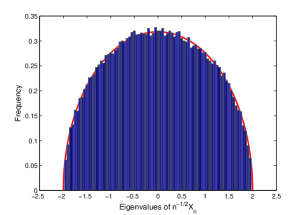
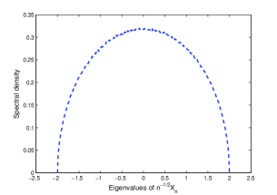
Figure 1: Limiting skew-spectral distribution for $G_{n,p}^{\sigma(q)}$ with $n=1000$, $p=0.1$ and $q=0.5$. (a) Histogram of the spectrum of $n^{-1/2}X_{n}$. A solid line shows the semicircular distribution for comparison. (b) The average spectral density for $n^{-1/2}X_{n}$ over 500 graphs.

References

• [1] S. E. Alm, S. Janson, S. Linusson, Correlations for paths in random orientations of $G(n,p)$ and $G(n,m)$. Random Struct. Algor., 39(2011) 486–506.
• [2] S. E. Alm, S. Linusson, A counter-intuitive correlation in a random tournament. Combin. Probab. Comput., 20(2011) 1–9.
• [3] Z. Bai, Methodologies in spectral analysis of large dimensional random matrices, a review. Statist Sinica, 9(1999) 611–677.
• [4] Z. Bai, J. Hu, W. Zhou, Convergence rates to the Marchenko-Pastur type distribution. Stoch. Proc. Appl., 122(2012) 68–92.
• [5] Z. Bai, J. W. Silverstein. Spectral Analysis of Large Dimensional Random Matrices. Springer, New York, 2010.
• [6] B. BollobΓ‘s, Random Graphs. Cambridge University Press, Cambridge, 2001.
• [7] A. Bose, S. Gangopadhyay, A. Sen, Limiting spectral distribution of $XX^{\prime}$ matrices. Ann. Inst. H. Poincare Probab. Statist., 46(2010) 677–707.
• [8] M. Cavers, S. M. Cioabǎ, S. Fallat, D. A. Gregory, W. H. Haemers, S. J. Kirkland, J. J. McDonald, M. Tsatsomeros, Skew-adjacency matrices of graphs. Linear Algebra Appl., 436(2012) 4512–4529.
• [9] X. Chen, X. Li, H. Lian, The skew energy of random oriented graphs. Linear Algebra Appl., 438(2013) 4547–4556.
• [10] X. Chen, X. Li, H. Lian, Lower bounds of the skew spectral radii and skew energy of oriented graphs. Linear Algebra Appl., 479(2015) 91–105.
• [11] S. Dallaporta, V. Vu, A note on the central limit theorem for the eigenvalue counting function of Wigner matrices. Electron. Commun. Probab., 16(2011) 314–322.
• [12] X. Ding, T. Jiang, Spectral distributions of adjacency and Laplacian matrices of random graphs. Ann. Appl. Probab., 20(2010) 2086–2117.
• [13] G. R. Grimmett, Infinite paths in randomly oriented lattices. Random Struct. Algor., 18(2001) 257–266.
• [14] Y. Hou, T. Lei, Characteristic polynomials of skew-adjacency matrices of oriented graphs. Electron. J. Combin., 18(2011) #P156.
• [15] S. Linusson, M. Leander, Correlation of paths between distinct vertices in a randomly oriented graph. Math. Scand., 116(2015) 287–300.
• [16] T. H. Marshall, On oriented graphs with certain extension properties. Ars Combin., 120(2015) 223–236.
• [17] C. McDiarmid, General percolation and random graphs. Adv. Appl. Probab., 13(1981) 40–60.
• [18] F. Rubio, X. Mestre, Spectral convergence for a general class of random matrices. Stat. Probab. Lett., 81(2011) 592–602.
• [19] B. Shader, W. So, Skew spectra of oriented graphs. Electron. J. Combin., 16(2009) #N32.
• [20] Y. Shang, Large dicliques in a directed inhomogeneous random graph. Int. J. Comput. Math., 90(2013) 445–456.
• [21] Y. Shang, Groupies in multitype random graphs. SpringerPlus, 5(2016) art. 989.
• [22] H. Weyl, Das asymptotische Verteilungsgesetz der Eigenwerte linearer partieller Differentialgleichungen. Math. Ann., 71(1912) 441–479.
• [23] E. P. Wigner, On the distribution of the roots of certain symmetric matrices. Ann. Math., 67(1958) 325–327.