Nonlocality of relaxation rates in disordered landscapes

Abstract

We investigate both analytically and by numerical simulation the relaxation of an overdamped Brownian particle in a 1D multiwell potential. We show that the mean relaxation time from an injection point inside the well down to its bottom is dominated by statistically rare trajectories that sample the potential profile outside the well. As a consequence, also the hopping time between two degenerate wells can depend on the detailed multiwell structure of the entire potential. The nonlocal nature of the transitions between two states of a disordered landscape is important for the correct interpretation of the relaxation rates in complex chemical-physical systems, measured either through numerical simulations or experimental techniques.

I Introduction

The problem of time relaxation around a local minimum of a free-energy landscape is ubiquitous in chemical physics. In fact, the landscape picture goldstein assumes a natural separation of low-temperature molecular motion sampling distinct potential energy minima, and vibration within a minimum. The manner in which a disordered material samples its landscape as a function of temperature thus provides information on its long-time relaxation properties. The energy landscape paradigm has been successfully applied to protein folding frauen , the mechanical properties of glasses malandro , and the dynamics of supercooled liquids sastry .

In this context, Adam-Gibbs’ formula adam suggests a phenomenological connection between kinetics and thermodynamics in disordered systems, that is, $\tau=A\exp(B/Ts_{c})$, where $\tau$ is a relaxation time, $A$ and $B$ are two phenomenological constants, and $s_{c}$ is a configurational entropy factor related to the number of minima of the system’s multidimensional energy surface. For instance, at low enough temperatures the system becomes stuck in a single minimum, the depth of which increases as the cooling rate decreases: this describes a glass transition. In this context, of prominent interest is the case of relaxation between two degenerate free-energy minima separated by an (almost) symmetric activation barrier. In the current literature this is referred to as the Kramers’ problem borkovec . In calculating the average transition time between two such states, one typically ignores the presence of other possible less stable (more energetic) states in the free-energy landscape tang . We show that statistically rare trajectories that connect two such degenerate states only after entering another neighboring state, are responsible for an increase of the relevant mean transition time, sometimes by orders of magnitude. The consequence is that in order to ignore the contribution of slowly meandering trajectories and keep using the results of standard Kramers’ theory, one has to restrict the system’s phase-space volume defining the free-energy stable states.

Our conclusion has an immediate counterpart and, hopefully, application in the strategies of path sampling for the numerical investigation of complex systems ferrario ; bowman . For instance, an unfolded protein can explore thousands of intermediate structures (conformations) before reaching a long-lived (stable) folded conformation. The most numerically efficient approach to investigate this process involves simulating protein folding with molecular dynamics for a relatively short time, and then analyzing the resulting trajectories to extract a coarse-grained Markov state model (MSM). An MSM consists of an appropriate choice of long-lived clustered conformational states and the transition rates between them. To create an MSM, one runs molecular dynamics simulations to determine how frequently a protein changes from one state to another, and clusters intermediate structures based on kinetic proximity (e.g., how energetically easy is switching from one structure to another). The transition rates are typically determined by averaging the time the protein takes to switch between any two states encoded in the MSM. Due to the coarse-grained nature of the MSM, a continuous trajectory connecting a pair of sampled states might well enter first the phase-space basin belonging to another state without being trapped there. This occurrence, though unlikely, may dramatically affect the corresponding transition time. How to correctly generate the reactive trajectories representing a specific transition of interest for the MSM is an issue of ongoing research.

The contents of this paper is organized as follows. In Sec. II we first simulate the relaxation of an overdamped Brownian particle in a 1D potential well. We determine both numerically and analytically the mean first-passage time (MFPT) for the particle to reach the bottom of the well from an injection point inside it. We show that when the injection point rests inside the well, but higher than the bottom of another adjacent well, then the rare trajectories crossing the barrier separating the two wells become dominant and, on lowering the noise level, the MFPT increases exponentially. Some of the results presented here have been independently derived in Ref. AA for discrete stochastic models of biological interest. In Sec. III we interpret this effect by distinguishing between two types of trajectories, the most probable trajectories pointing from the injection point straight down to the well bottom, and the rare trajectories overcoming the barrier into the side well. The distribution density of the relaxation times allows a clear-cut distinction between these two types of trajectories. In Sec. IV we extend our analysis to the case of multiwell potentials and conclude that the MFPT inside a well is dominated by barrier-crossing anytime the particle’s injection point rests above the level of the lowest lying among all adjacent wells (Sec. IV.1). Finally, we consider the case of the hopping process between two degenerate minima of the potential and discuss how the MFPT over the barrier separating them can depend on the level of the injection point and, therefore, on the multistable structure of the entire potential (Sec. IV.2). In Sec. V we draw some concluding remarks regarding the impact of this effect on the interpretation of actual relaxation measurements.

II Relaxation times in a bistable potential

We start introducing two categories of trajectories a 1D system may take while relaxing toward a stable state. Broadly speaking, we distinguish between regular trajectories, the most probable and typically the shortest ones, given certain initial conditions, and a subset of dominant trajectories, which one determines with reference to the observable being measured. The most probable transition trajectories in a 1D system has been classified by analyzing the (local) minima of the relevant action integrals path1 ; path3 . Here, we are rather concerned with identifying the systems’ trajectories that most contribute to the mean value of a specific observable of interest.

A study-case is represented by the transition times $t(a,x_{0})$ of an overdamped Brownian particle obeying the Langevin equation (LE),

$$\dot{x}=-V^{\prime}(x)+\xi(t),$$ (2.1)

where $x(t)$ denotes the particle coordinate, $V(x)$ is a confining multistable potential, and $\xi(t)$ models a stationary, zero-mean, Gaussian noise source with autocorrelation function

$$\langle\xi(t)\xi(0)\rangle=2D\delta(t).$$ (2.2)

The particle will be injected at a given point $x_{0}$ and taken out upon reaching the exit point $x_{a}$. To keep our notation as simple as possible, we place the exit point at the bottom of a potential well, termed well $a$, located on the left of the injection point, i.e., $x_{a}<x_{0}$, see inset of Fig. 1. The time length of each trajectory is the observable of interest, $t(a,x_{0})$.

The average transition time $T(a,x_{0})\equiv\langle t(a,x_{0})\rangle$ for the particle to diffuse from $x_{0}$ to $a$, is given by the well-known MFPT formula stratonovich ; gardiner ; goel ,

$$T(a,x_{0})=\frac{1}{D}\int_{x_{a}}^{x_{0}}\frac{dy}{p(y)}\int_{y}^{\infty}p(z)dz,$$ (2.3)

where $p(x)={\cal N}\exp[-V(x)/D]$ is the stationary probability density of the process (2.1). Note that for a confining potential, $\lim_{x\to\pm\infty}p(x)=0$, i.e., $x\to\infty$ can be treated as a reflecting boundary gardiner

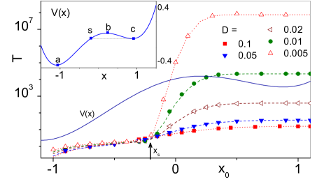
Figure 1: (Color online) Mean first-passage time $T=T(a,x_{0})$ vs. $x_{0}$ from numerical integration of the LE (2.1) with the asymmetric bistable potential $V(x)=x^{4}/4-x^{2}+x/5$ (inset) and different noise strength, $D$. The potential minima are located at $x_{a}\approx-1.088$ and $x_{c}\approx 0.879$, the barrier at $x_{b}\approx 0.209$, and the crossover threshold, defined by $V(x_{s})=V_{c}$, at $x_{s}\approx-0.204$. The dashed curves $T(a,x_{0})$ were obtained by performing the double integral in Eq. (2.4) for the appropriate $D$.

We specialize now Eq. (2.3) to the case of an asymmetric bistable potential. As illustrated in the inset of Fig. 1, $x_{b}$ locates the top of the barrier, $b$, and $x_{a}$ and $x_{c}$ denote the bottom of the left, $a$, and right well, $c$, respectively, with $V_{a}<V_{c}$. Here and in the following, we adopted the short-hand notation $V(x_{a})=V_{a}$, $V(x_{b})=V_{b}$, $V(x_{c})=V_{c}$, $V(x_{0})=V_{0}$, and prime for an $x$ derivative, $(\dots)^{\prime}=d(\dots)/dx$. The threshold $x_{s}$ is the point on the r.h.s. of $a$ that has the same potential energy as the bottom of well $c$; for the asymmetric double-well potential of Fig. 1, $V(x_{s})=V_{c}$ with $x_{s}>x_{a}$.

We then estimate the MFPT (2.3) in the weak noise limit, $D<V_{b}-V_{c}$, for three different ranges of the injection point, $x_{0}$:

(i) out-of-well, $x_{0}>x_{b}$. The functions $p(x)$ and $p^{-1}(x)$ are sharply peaked, respectively, around points $x_{a}$ and $x_{c}$ and around point $x_{b}$. As a consequence, for $x_{0}>x_{b}$ the nested integrals (2.3) factorize, that is,

$$T(a,x_{0})=\frac{1}{D}\int_{x_{a}}^{x_{0}}\frac{dy}{p(y)}\int_{x_{b}}^{\infty}p(z)dz.$$ (2.4)

In the limit of weak noise gardiner $p(z)/p(y)\simeq\exp[(V_{b}-V_{c})/D-|V_{b}^{\prime\prime}|(x-x_{b})^{2}/2D-V_{c}^{\prime\prime}(x-x_{c})^{2}/2D]$, so that the integrals (2.4) can be approximated to

$$T(a,x_{0})=\frac{2\pi}{\sqrt{|V_{b}^{\prime\prime}|V_{c}^{\prime\prime}}}\exp\left(\frac{V_{b}-V_{c}}{D}\right).$$ (2.5)

This is the well-known Kramers’ formula, $T_{K}(a,c)$, for the escape time out of well $c$. Here, according to our notation, all escape trajectories are regular and the ensuing (almost $x_{0}$ independent) relaxation time is characterized by the slow relaxation process $x_{c}\to x_{a}$.

(ii) barrier well region, $x_{s}<x_{0}<x_{b}$. For this choice of the injection point, the first integrand (2.4) can be approximated to $p^{-1}(y)\simeq\exp[V_{0}/D+V_{0}^{\prime}(y-x_{0})/D]$; hence

$$T(a,x_{0})=\frac{1}{|V_{0}^{\prime}|}\sqrt{\frac{2\pi D}{V_{c}^{\prime\prime}}}\exp\left(\frac{V_{0}-V_{c}}{D}\right).$$ (2.6)

Here we took the absolute value of $V_{0}^{\prime}$ only for the sake of generality. This result is suggestive: Although the particle was injected directly in well $a$, still it takes an exponentially long average time to reach its bottom, $x_{a}$. Moreover, in contrast with Kramers’ time of Eq. (2.5), $T(a,x_{0})$ appears to depend on how high the injection point lies with respect to the minimum, $V_{c}$, of the side-well $c$. As discussed in Sec. III, the MFPT (2.6) is indeed dominated by the rare trajectories that cross over into well $c$ before being absorbed at $x_{a}$.

(iii) bottom well region, $x_{0}<x_{s}$. As $x_{0}$ approaches the exit point, one can easily take the $x_{0}\to x_{a}$ limit of the double integral (2.3), thus obtaining the logarithmic law,

$$T(a,x_{0})=\frac{1}{2V^{\prime\prime}_{a}}\left[2\ln 2+\gamma+\ln\left(\frac{V_{0}-V_{a}}{D}\right)\right],$$ (2.7)

where $\gamma\simeq 0.577$ is the Mascheroni’s constant. This is the short MFPT one would expect on account of the sole regular trajectories of the relaxation process. Indeed, such trajectories run straight downhill from $x_{0}$ subject to weak noise fluctuations, whose effect grows appreciable only close to the exit point, $x=x_{a}$.

Our analytical estimates (2.5)-(2.7) reproduce well the three different regimes of the $T(a,x_{0})$ curves of Fig. 1, obtained by numerically computing the double integral (2.3) for very small $D$ values. The crossover between the logarithmic (2.7) and the exponential branch (2.6) of $T(a,x_{0})$ is fairly sharp, because the exponential in Eq. (2.6) abruptly vanishes for $x_{0}<x_{s}$ and $|V_{0}-V_{c}|\ll D$.

In passing we notice that our approximations (2.5) and (2.6) coincide (apart from minor typographical errors) with the first two MFPT’s reported in Eq. (33) of Ref.AA for Schlögl’s model in the large size system limit. Our derivation is much simpler, indeed, but restricted to the case of continuous stochastic transition processes.

Finally, the results of this section can be readily extended to the case when the side-well $c$ is deeper than the exit well, $V_{c}<V_{a}$. Only approximation (2.7) needs to be modified as the probability density, $p(x)$, in the exit well gets exponentially suppressed. As a consequence, the right hand side of Eq. (2.7) must be multiplied by the additional factor $\exp[(V_{a}-V_{c})/D]$. This means that, since no threshold $x_{s}$ could be defined, the average transition time is exponentially long for any in-well injection point, namely, $T(a,x_{0})\propto\exp[(V_{0}-V_{c})/D]$ for $x_{a}<x_{0}<x_{b}$.

III The role of the dominant trajectories

As anticipated in the foregoing section, the results of Eqs. (2.5) and (2.7) lend themselves to a simple interpretation in terms of regular trajectories. For $x_{0}>x_{b}$ the particle is initially placed in the side-well $c$, so that it, first, relaxes around the local $p(x)$ maximum at $x_{c}$ and, then, escapes into well $a$ by overcoming the barrier $b$; as a consequence $T(a,x_{0})$ is quite insensitive to the injection point $x_{0}$. For $x_{a}<x_{0}<x_{s}$ the particle tends to roll downhill toward the exit point $x_{a}$, corresponding to the absolute maximum of $p(x)$, with a short average transition time proportional to the logarithm of the initial displacement, $x_{0}-x_{a}$.

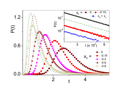
Figure 2: (Color online) Distribution densities, $P(t)$, of the transient times $t=t(a,x_{0})$ obtained by numerically integrating the LE (2.1) for the asymmetric bistable potential of Fig. 1 with $D=0.01$ and different $x_{0}$. The dashed curves represent the harmonic approximation $P_{s}(t)$ of Eq. (3.5) for the two $x_{0}$ closest to $x_{a}$, see text. Inset: semi-logarithmic plot of $P(t)$ vs $t$ for three values of $x_{0}$  and $D=0.01$. The three data sets are closely fitted by the function $P_{l}(t)$ in Eq. (3.4). The dashed line with $T_{K}(x_{a},x_{0})$ has been drawn to guide the eye.

The transitions that start out in the barrier region $x_{s}<x_{0}<x_{b}$ are qualitatively different. As the injection point lies inside well $a$, the trajectories oriented toward the exit point are still the most probable, or, stated otherwise, they represent the process’ regular trajectories, as expected. Nevertheless, the particle can diffuse from $x_{0}$ over the barrier into well $c$ with small but finite probability. Following Refs. gardiner ; goel , we can estimate the splitting probability $\pi(a,x_{0})$ for the particle to exit at $a$ without first reaching $c$, and $\pi(c,x_{0})$ for the particle to fall into well $c$ before being absorbed at $a$,

$$\pi(c,x_{0})=1-\pi(a,x_{0}),$$ (3.1)

$$\pi(a,x_{0})=\int_{x_{0}}^{x_{c}}\frac{dy}{p(y)}{\large/}\int_{x_{a}}^{x_{c}}\frac{dy}{p(y)}.$$ (3.2)

For weak noises and $x_{0}$ not too close to the extrema $x_{a}$ and $x_{b}$, the integral (3.2) can be approximated to gardiner

$$\pi(c,x_{0})\simeq\frac{1}{|V_{0}^{\prime}|}\sqrt{\frac{D|V_{b}^{\prime\prime}|}{2\pi}}\exp\left(\frac{V_{0}-V_{b}}{D}\right).$$ (3.3)

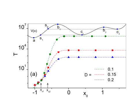
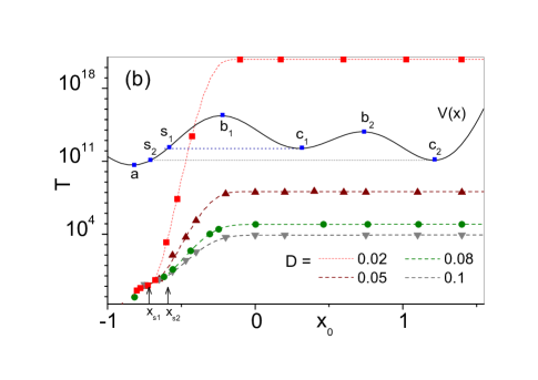
Figure 3: (Color online) Mean first-passage time $T=T(a,x_{0})$ vs. $x_{0}$ in the asymmetric three-well potentials (a) $V(x)=x^{4}/2-x^{2}-0.7\sin(4.5x)$ and (b) $V(x)=x^{4}/2-x^{2}-0.35\sin(6x)$ for different $D$. Note that in (a) $V_{c_{1}}<V_{c_{2}}$ and in (b) $V_{c_{1}}>V_{c_{2}}$; in both cases $V_{a}<V_{c_{i}}$, $i=1,2$. The data points are the result of the numerical integration of LE (2.1) for the relevant choices of $V(x)$ and $D$; the dashed curves are the corresponding analytical expressions of Eq. (2.4).

Although the typical trajectories are by far the most probable – being $\pi(a,x_{0})\simeq 1$, – still their contribution to the average transition time $T(a,x_{0})$ is negligible, as they reach the exit point in a quite short time, see Eq. (2.7). By contrast, the barrier crossings may well be very unlikely – being $\pi(c,x_{0})$ exponentially small, – but the particle, after falling into well $c$, takes an exponentially long time of the order of $T_{K}(a,c)$ [see Eq. (2.3) for $x_{0}=c$], to recross into well $a$. The contribution to $T(a,x_{0})$ from such rare trajectories amounts to $\pi(c,x_{0})T_{K}(a,c)$, that is, to our estimate in Eq. (2.6). In conclusion, as long as we characterize the relaxation in the overdamped potential $V(x)$ by measuring the exit times, $t(a,x_{0})$, the otherwise sporadic trajectories crossing the barrier may become dominant, depending on the injection point. Of course, this argument only applies for small, but finite noise strengths, i.e., $D\to 0+$, whereas in the noiseless regime, $D=0$, there exists only one allowed deterministic trajectory running downhill from $x_{0}$ to $x_{a}$ for any $a<x_{0}<x_{b}$.

In real or numerical experiments one can easily sample relaxation trajectories from $x_{0}$ to $x_{a}$ and distribute them according to their temporal length, $t(a,x_{0})$. Based on the argument above, where the regular trajectories are regarded as much faster than the dominant ones, the $t$-distribution density, $P[t(a,x_{0})]$, can be separated into two distinct terms, i.e., $\pi(a,x_{0})P_{s}(t)+\pi(c,x_{0})P_{l}(t)$. For the sake of a comparison with actual data, in the regime of weak noise one can introduce the approximations,

$$P_{l}(t)\simeq\frac{T(a,x_{0})}{T_{K}^{2}(a,c)}\,\exp[-{t}/{T_{K}(a,c)}],$$ (3.4)

for the long exit times of the statistically rare trajectories crossing the barrier, and

$$P_{s}(t)\simeq-\frac{2}{\sqrt{\pi}}\frac{d}{dt}\left[\frac{V_{0}-V_{a}}{D(t)}\right]^{\frac{1}{2}}\cdot\exp[-({V_{0}-V_{a}})/{D(t)}],$$ (3.5)

with $D(t)=e^{2V_{a}^{\prime\prime}t}-1$, for the intrawell relaxation trajectories. Our expression for $P_{s}(t)$ holds good for the harmonic approximation of the potential well $a$, that is, by setting $V(x)=V_{a}+(1/2)V_{a}^{\prime\prime}(x-x_{a})^{2}$ and ignoring all anharmonic terms of the third order and higher. It was derived by standard MFPT methods gardiner and can be reformulated to match earlier solutions for $t$-distribution in a harmonic well szabo ; berne . In Eq. (3.4) for $P_{l}(t)$, we approximated the probability of barrier crossing as $\pi(c,x_{0})\simeq T(a,x_{0})/T_{K}(a,c)$, and made use of the well-established exponential distribution for Kramers’ escape times from $c$ back to $a$ borkovec ; gardiner ; goel .

In Fig. 2 we display the outcome of an extensive numerical simulation of the exit process, Eq. (2.1), for the potential of Fig. 1 and different values of $D$. As the injection point is shifted past the threshold $x_{s}$, also the relaxation time distributions change abruptly. An exponential tail associated with the dominant trajectories becomes visible for $x_{0}\geq x_{s}$ (inset); as predicted in Eq. (3.4), such a tail has a small amplitude of the order of $T(a,x_{0})/T_{K}^{2}(a,c)$ and decays slowly with time constant $T_{K}(a,c)$. The distributions of the short relaxation times due to the regular trajectories, main panel, are reminiscent of the $t$-distributions in a harmonic well, $P_{s}(t)$ of Eq. (3.5). However, the agreement gets quantitatively close only when $x_{0}$ approaches $x_{a}$, the convergence being rather slow. We attributed this inconvenience to the spatial asymmetry of well $a$. Moreover, we remark that the average $\langle t(a,x_{0})\rangle$ taken over the regular trajectories only, namely by using the approximate distribution density Eq. (3.5), is a monotonic decreasing function of $D$; for vanishingly small $D$ values it comes close to the predicted estimate in Eq. (2.7).

IV Generalization to multiwell potentials

The results of Sec. II can be extended to study transitions in multiwell potentials, as well. However, the algebraic manipulations on the MFPT (2.3) can become more complicated due to the multi-peaked structure of the functions $p(x)$ and $p^{-1}(x)$. Luckily, to gain a better understanding of the role of the dominant trajectories in the most general case of a disordered potential, it suffices to analyze in some detail the three-well potentials, only. While any disordered potential can be regarded as an appropriate sequence of three-well potentials, it is clear that the relaxation properties discussed below only apply in the limit of infinite observation times, where the diffusing particle is allowed to explore the entire potential profile. Shorter observation times would necessarily restrict our analysis to the portion of the potential profile actually accessed by the particle.

IV.1 Nondegenerate three-well potentials

Let us imagine to add a third well to the potential plotted in Fig. 1. If we agree on that the exit well must be at the bottom of the lowest one, then two geometries are possible, as illustrated in Fig. 3. Let $c_{1}$ and $c_{2}$ denote, respectively, the first and the second well to the right of well $a$, with barriers $b_{1}$ and $b_{2}$ separating the three wells. As for both wells $V_{c_{i}}>V_{a}$, with $i=1,2$, the equations $V(x_{s_{i}})>V_{c_{i}}$ may define two thresholds, $x_{s_{i}}$, with $a<x_{s_{i}}<x_{b_{1}}$. As a consequence, the barrier region of well $a$ is delimited from below by the threshold $\overline{x}_{s}\equiv\min\{x_{s_{i}}\}$, that is, it starts at the level of the lower side-well $c_{i}$ – see the geometric constructions in panels (a) and (b).

Now, the question rises naturally whether, in the presence of two (or more) thresholds, the slope of $T(a,x_{0})$ changes at each of them, and where such changes are possibly the most pronounced. The answer is illustrated in the two panels of Fig. 3, where the MFPT (2.3) has been plotted over an $x_{0}$ range comprising both $x_{s_{i}}$: On reducing the noise intensity, a sharp crossover between a logarithmic and an exponential $x_{0}$ dependence emerges in the neighborhood of $\overline{x}_{s}$, whereas no substantial MFPT change can be associated with the other threshold. This conclusion can be confirmed qualitatively by extending the semi-quantitative approach of Sec. II to both potentials of Fig. 3. In the barrier region, the average transient time $T(a,x_{0})$ is dominated by the lower side-well $c_{i}$; the dominant trajectories cross one or two barriers, depending on which side-well is deeper. Accordingly, in the barrier region $\overline{x}_{s}<x_{0}<x_{b_{1}}$, the curve $T(a,x_{0})$ grows proportional to $\exp([V_{0}-V(\overline{x}_{s})]/D)$. Note that in view of the remark at the bottom of Sec. II, should one side-well $c_{i}$ sit lower than well $a$, then such an exponential dependence would apply throughout the entire range $x_{a}<x_{0}<x_{b_{1}}$ and no logarithmic-to-exponential crossover would occur.

IV.2 Degenerate three-well potentials

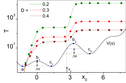
Figure 4: (Color online) Mean first-passage time $T=T(a,x_{0})$ vs. $x_{0}$ in the degenerate three-well potential $V(x)=\cos 2x-\cos x++0.1x$ for different $D$; simulation (symbol) versus analytical results (dashed curves). Note that $V_{a}=V_{c_{1}}$ and the threshold $x_{0}=x_{s}$ is defined by the condition $V(x_{s})=V_{c_{2}}+\Delta V$, where $\Delta V=V_{b_{1}}-V_{c_{1}}$ (see text). The dashed curves were obtained by numerically integrating Eq. (2.4) for the three-well potential.

We consider now the special case of a three-well potential with two degenerate lower minima, say, in $x_{a}$ and $x_{c_{1}}$, see Fig. 4. This means that wells $a$ and $c_{1}$ are equally deep, while the third well sits higher up, that is, $V_{a}=V_{c_{1}}<V_{c_{2}}$. Then, the process (2.1) models the relaxation occurring between two degenerate states, a mechanism often invoked in the chemical physical literature. As discussed in Sec. I, for low noise levels this problem is commonly addressed by ignoring the presence of more energetic states in the neighborhood. However, the remarkable dependence of $T(x_{0},a)$ on the injection point, $x_{0}$, shown in figure, suggests a different picture. As long as $x_{0}$ is confined around the bottom of well $c_{1}$, the MFPT from $x_{0}$ to $x_{a}$ is almost independent of $x_{0}$ and well reproduced by the Kramers’ rate of Eq. (2.5) upon replacing $x_{0}$ with $c_{1}$, and $b$ with $b_{1}$. In this case the role of well $c_{2}$ is irrelevant. However, on moving $x_{0}$ to the right of a certain threshold $x_{s}$, $T(x_{0},a)$ suddenly jumps up to a much higher value, insensitive to any further increase of $x_{0}$.

The location of the threshold point $s$ and the magnitude of the MFPT jump can be explained as follows. We assume that the lower $T(x_{0},a)$ plateau for $x_{b_{1}}<x_{0}<x_{s}$ is due to the regular trajectories crossing from $c_{1}$ to $a$ directly over barrier $b_{1}$ and, therefore, proportional to $\exp(V_{b_{1}}-V_{c_{1}})$, whereas the higher plateau must come from those rare trajectories that cross first barrier $b_{2}$ to the right, with probability proportional to $\exp[-(V_{b_{2}}-V_{0})]$. The time they take to cross back from well $c_{2}$ to well $c_{1}$ (and then to well $a$) is a Kramers’s time proportional to $\exp(V_{b_{2}}-V_{c_{2}})$. Therefore, their weighted contribution to the MFPT is proportional to $\exp(V_{0}-V_{c_{2}})$ and, most remarkably, supersedes the contribution from the regular trajectories for $V_{0}-V_{c_{2}}>V_{b_{1}}-V_{c_{1}}$. Accordingly, $x_{s}$ is determined by choosing $V(x_{s})=V_{c_{2}}+\Delta V$, where $\Delta V=V_{b_{1}}-V_{c_{1}}$ is the barrier height separating wells $a$ and $c_{1}$ – see the geometric construction in Fig. 4.

As long as $V(x_{s})<V_{b_{2}}$, the threshold $x_{s}$ is well defined. Therefore, there can exist a barrier region inside well $c_{1}$, $x_{s}<x_{0}<x_{b_{2}}$, such that the relaxation trajectories creeping into well $c_{2}$ are indeed dominant. The corresponding $t$-distributions are well fitted by double exponential functions (not shown) with decay constants equal to the two plateau values of the curves $T(x_{0},a)$ versus $x_{0}$.

V Conclusions

Many systems in condensed matter are described by an overdamped particle that diffuses on a disordered energy landscape of appropriate dimensionality, without ever reaching a proper equilibrium state (glassy materials are a good example). The physical chemical properties of these systems are often interpreted in terms of the relaxation rates inside single locally stable states or between pairs of locally stable states. However, determining such rates experimentally, through microscopic techniques, or even numerically, may prove a moot problem. As discussed in Secs. II and IV, the investigator who intends to proceed by weakly exciting the system out of its locally stable state and then letting it relax back to it, may encounter the difficulty of establishing whether the measured relaxation time depends on the presence of other metastable states. This difficulty can be circumvented by a more restrictive definition of locally stable state.

Our analysis clearly shows that in 1D the relaxation times within a single potential well or between degenerate wells can be determined by ignoring additional potential wells only under the condition that the energy of what we call the injection point is sufficiently close to the energy of the well bottom. How close, it depends on the actual distribution of the wells along the potential landscape. Indeed, the critical threshold is determined by the lowest lying well, an information usually unavailable to the investigator. Therefore, above a certain (but unknown) threshold of the injection energy, the measured relaxation times exhibit a marked nonlocal dependence on the global potential profile. Such a nonlocal effect is due to the contribution from slower, though rare, relaxation trajectories, which explore the potential landscape surrounding the well(s) of interest. Their presence can be appreciated, for instance, by looking at the distribution of the relevant relaxation times, though at the expense of much longer observation times.

The present analysis was restricted to 1D potentials for the sake of clarity, thus making our presentation hopefully easier to follow and affording higher numerical statistics. Its extension to potentials in two and even higher dimensions confirms the overall picture summarized here and is presently matter of further investigation.

References

- (1) M. Goldstein, Viscous liquids and the glass transition: a potential energy barrier picture, J. Chem. Phys. 51, 3728 (1969).
- (2) H. Frauenfelder, S. G. Sligar, and P. G. Wolynes, The energy landscapes and motions of proteins, Science 254 1598 (1991).
- (3) D. L. Malandro, and D. J. Lacks, Relationships of shear-induced changes in the potential energy landscape to the mechanical properties of ductile glasses, J. Chem. Phys. 110, 4593 (1999).
- (4) S. Sastry, P. G. Debenedetti, and F. H. Stillinger, Signatures of distinct dynamical regimes in the energy landscape of a glass-forming liquid, Nature 393, 554 (1998).
- (5) G. Adam and J. H. Gibbs, On the temperature dependence of cooperative relaxation properties in glass-forming liquids, J. Chem. Phys. 43 139 (1965).
- (6) P. Hänggi, P. Talkner, and M. Borkovec, Reaction-rate theory: fifty years after Kramers, Rev. Mod. Phys. 62 251 (1990).
- (7) L. Luo and L.-H. Tang, Sample-dependent first-passage-time distribution in a disordered medium, Phys. Rev. E 92, 042137 (2015).
- (8) G. R. Bowman, V. S. Pande, and F. Noé (Eds.), An Introduction to Markov state models and their application to long timescale molecular simulation (Springer, Dordrecht, 2014).
- (9) M. Ferrario, G. Ciccotti, and K. Binder (Eds.), Physics Computer Simulations in Condensed Matter Systems: From Materials to Chemical Biology Volume 1, Lect. Notes Phys. 703 (Springer, Berlin Heidelberg 2006).
- (10) C. R. Doering, K. V. Sargsyan, L. M. Sander, and E.Vanden-Eijnden, Asymptotics of rare events in birth-death processes bypassing the exact solutions, J. Phys. Condens. Matter 19, 065145 (2007).
- (11) B. E. Vugmeister, J. Botina, and H. Rabitz, Nonstationary optimal paths and tails of prehistory probability density in multistable stochastic systems, Phys. Rev. E 55, 5338 (1997).
- (12) S. M. Soskin, Most probable transition path in an overdamped system for a finite transition time, P hys. Lett. A 353, 281 (2006), and additional references therein.
- (13) R. L. Stratonovich, Radiotekh. Electron. (Moscow) 3, 497 (1958). English translation in Non-Linear Transformations of Stochastic Processes, edited by P. I. Kuznetsov, R. L. Stratonovich, and V. I. Tikhonov (Pergamon, Oxford, 1965).
- (14) C. W. Gardiner Handbook of Stochastic Methods (Springer, Berlin, 1985). Chapters 5 and 9.
- (15) N. Goel and N. Richter-Dyn, Stochastic Models in Biology (Academic Press, New York, 1974).
- (16) A. Szabo, K. Schulten, and Z. Schulten, First passage time approach to diffusion controlled reactions, J. Chem. Phys. 72, 4350 (1980).
- (17) Z. Hu, L. Cheng, and B. J. Berne, First passage time distribution in stochastic processes with moving and static absorbing boundaries with application to biological rupture experiments, J. Chem. Phys. 133, 034105 (2010).