The not so simple globular cluster $\omega$ Cen. I. Spatial distribution of the multiple stellar populations.

Abstract

We present a multi-band photometric catalog of $\approx$ 1.7 million cluster members for a field of view of $\approx$ 2$\times$2^∘ across $\omega$ Cen. Photometry is based on images collected with the Dark Energy Camera on the 4m Blanco telescope and the Advanced Camera for Surveys on the Hubble Space Telescope. The unprecedented photometric accuracy and field coverage allowed us for the first time to investigate the spatial distribution of $\omega$ Cen multiple populations from the core to the tidal radius, confirming its very complex structure. We found that the frequency of blue main-sequence stars is increasing compared to red main-sequence stars starting from a distance of $\approx$ 25’ from the cluster center. Blue main-sequence stars also show a clumpy spatial distribution, with an excess in the North-East quadrant of the cluster pointing towards the direction of the Galactic center. Stars belonging to the reddest and faintest red-giant branch also show a more extended spatial distribution in the outskirts of $\omega$ Cen, a region never explored before. Both these stellar sub-populations, according to spectroscopic measurements, are more metal-rich compared to the cluster main stellar population. These findings, once confirmed, make $\omega$ Cen the only stellar system currently known where metal-rich stars have a more extended spatial distribution compared to metal-poor stars. Kinematic and chemical abundance measurements are now needed for stars in the external regions of $\omega$ Cen to better characterize the properties of these sub-populations.

1. Introduction

The peculiar Galactic Globular Cluster (GGC) $\omega$ Cen (NGC 5139) has been subject to substantial observational efforts covering the whole wavelength spectrum from the ultraviolet to the near-infrared. This gigantic star cluster, the most massive known in our Galaxy, $M=2.5\times 10^{6}$ $M_{\odot}$(van de Ven et al., 2006) has (at least) three separate stellar populations with a large undisputed spread in metallicity (Norris & Da Costa, 1995; Norris et al., 1996; Suntzeff & Kraft, 1996; Kayser et al., 2006; Villanova et al., 2007; Calamida et al., 2009; Johnson & Pilachowski, 2010). Table 1 summarizes the basic parameters of $\omega$ Cen.

It has been suggested that $\omega$ Cen stellar populations not only show different chemical abundances but also have different kinematical properties. In particular, Norris et al. (1997) matching the spectroscopic abundances of $\approx$ 500 red-giant (RG) stars with the radial velocities by Mayor et al. (1997), observed that the metal-rich (MR) stars of $\omega$ Cen do not share the rotational velocity (V $\approx$ 8 Km s^-1) of the metal-poor (MP) component. The most MR stars also seem to have a smaller velocity dispersion compared to the MP stars. However, these results were questioned by Pancino et al. (2007) and Sollima et al. (2009), who found that the most MR stellar component of $\omega$ Cen does not present any significant radial velocity offset with respect to the bulk of stars. Moreover, the velocity dispersion profile appears to decrease monotonically from $\sigma_{v}\approx 17.2$ km/s down to a minimum value of $\sigma_{v}\approx 5.2$ km/s, in the region 1.5 $\leq r\leq$ 28’. For distances larger than 30’ an hint of a raise in the velocity dispersion is present, but this result is not statistically significant (Sollima et al., 2009).

A study of proper motions of the different cluster stellar populations was performed by Ferraro et al. (2002), who combined the proper motion data of van Leeuwen et al. (2000) with the photometry of Pancino et al. (2000). This analysis showed that the most MR stars in the cluster have a different motion compared to the metal-intermediate (MI) and MP stars. They suggested that the most MR stars in $\omega$ Cen formed in an independent stellar system later accreted by the cluster.

Pancino et al. (2000, 2003), by analyzing the spatial distribution of a sample of cluster RG stars, concluded that the three main stellar populations of $\omega$ Cen (MP, MI, and MR) have different distributions: MP stars are distributed along the direction of the cluster major axis (E–W), while the MI and MR along the N–S axis. This result was confirmed by Hilker & Richtler (2000), based on their Strömgren photometric metallicities for a sample of $\omega$ Cen RGs. In particular, they found that the more MR stars seem to be more concentrated within a radius of 10′  from the cluster center. Sollima et al. (2005) also found that MR stars are more centrally concentrated based on photometry of RG stars for a field of view (FoV) of $\approx$ 0.2$\times$0.2^∘ across the cluster.

Another peculiar property of $\omega$ Cen is the splitting of the main-sequence (MS). Hubble Space Telescope (HST) photometry revealed for the first time that $\omega$ Cen MS bifurcates into two main components, the so called blue-MS (bMS) and red-MS (Anderson, 2002; Bedin et al., 2004). Spectroscopic follow-up by Piotto et al. (2005) showed that bMs stars are more metal-rich than rMS stars, while their color being bluer. These authors then suggested that bMS stars constitute a helium-enhanced sub-population in the cluster. The split of $\omega$ Cen MS was also found by Sollima et al. (2007b) based on Very Large Telescope (VLT) photometry. They showed that the two sequences are still well-separated at $\approx$ 26′  from the cluster center and that the bMS is more centrally concentrated compared to the rMS.

The formation history and composition of $\omega$ Cen form a complex puzzle that is being slowly pieced together by investigations based on the latest generation of telescopes. However, all previous photometric studies were based on catalogs covering a field of view of no more than $\approx$ 40$\times$40′  across $\omega$ Cen. We now push forward the ongoing investigations by combining precise multi-band DECam photometry, covering $\approx$ 2$\times$2^∘ across the cluster, and HST data for the cluster center to characterize the properties of $\omega$ Cen multiple stellar populations from the core to the tidal radius.

The structure of the current paper is as follows. In §2 we discuss the observations and data reduction of DECam and ACS data of $\omega$ Cen. In §3 we illustrate the calibration strategy used for the ground-based data set and §4 deals with the selection criteria adopted to identify candidate field and cluster stars. In §5 we present the ground-based color-magnitude diagrams while in §6 we illustrate how we performed the astronometric calibration of our data set.

In §7 and 8 we discuss the spatial distribution of the different $\omega$ Cen stellar populations and we summarize and discuss the results in §9.

2. Observations and data reduction

Photometric data discussed in this investigation belong to two different sets from both space and ground based telescopes. A set of 57 ugri images centered on $\omega$ Cen was collected over 3 nights, 2014 February 24, 2015 June 22 and 2016 March 4, with the Dark Energy Camera (DECam) on the 4m Blanco Telescope (CTIO, NOAO). DECam is a wide-field imager with 62 CCDs and covers a 3 square degree sky FoV with a pixel scale of 0.263″. Exposure times for our observations ranged from 120 to 600s for the $u$-band and from 7 to 250s for the other filters. Weather conditions were very good for all nights with image seeing ranging from 0.8″  to 1.6″  for the $u$-band and from 0.7″  to 1.2″  for the other filters. Standard stars from the Sloan Digital Sky Survey (SDSS) Stripe 82 were observed in all filters and at different air masses for the night of February 2014. The accuracy of the derived zero points (ZPs) ranges between 2% for the $r$ and $i$ filters to $4-5$% for the $g$ and $u$ filters. For more details on the photometric calibration see Table 3 and Section §3. Table 2 lists the log of the DECam observations while Fig. 1 shows the footprint of DECam photometric catalog (black dots) for $\omega$ Cen. Note that stars are missing at the top and bottom of the footprint since 2 out of the 62 DECam ccds, N7 and S7, are not operational.

Photometry in the $F435W$, $F625W$, $F658N$ filters was collected with the Advanced Camera for Surveys (ACS) on board the Hubble Space Telescope (HST) for a region covering a FoV of $\approx 10\arcmin\times 9.5\arcmin$ centered on $\omega$ Cen. For more details about these observations see Castellani et al. (2007, hereafter CS07).

DECam images were pre-reduced by using a pipeline developed by one of us, Photpipe. Photpipe is a robust pipeline used by several time-domain surveys (e.g., SuperMACHO, ESSENCE, Pan-STARRS1; see Rest et al. 2005, 2014), designed to perform single-epoch image processing including image calibration. We used Photpipe to perform bias subtraction, flat-fielding, cross-talk correction, geometrical distortion correction and the image astrometric calibration.

Photometry was performed with a variant of DoPHOT (Schechter et al., 1993), with a pipeline developed by one of us for reducing DECam images along the lines described in Saha et al. (2010). DoPHOT uses an analytical function as a model point-spread function (PSF) for describing different object types. Aperture magnitudes are determined for bright isolated stars across each of the 60 operational chips of the camera. The difference between the PSF and aperture magnitudes is mapped over the field of view, accounting for chip to chip offsets, and this provides the correction factors for DoPHOT PSF magnitudes (see Saha et al. 2010, for details). The same reduction pipeline performs a few quality selections on the catalog: i) stars that lie too close to the chip borders, i.e. less than 20 pixels away, are excluded; ii) if a star has a close neighbor with significant comparative brightness is excluded; iii) stars with photometric errors more than 3 sigma the average photometric error for all objects in the corresponding 0.5 magnitude bin are excluded.

3. Photometric calibration

During the night of 2014 February 24, a Stripe82 field was observed in all the four filters, namely SDSS1048p0000. We retrieved the photometry for the stars included in this field from the Sloan Digital Sky Survey (SDSS) and from the Pan-STARRS1 (PS1) catalogs. To transform the photometry into the DECam natural system we followed the approach of Scolnic et al. (2015). We derived the transformations from PS1 and SDSS to the DECam system based on the photometry of 205 out of the 379 standard stars of the Next Generation Stellar Library (NGSL). These standard stars span a color range $-1.0\lesssim g-i\lesssim 2.5$ mag, and magnitudes are in the range $2\lesssim g\lesssim 12$ mag (for more details on how these stars were selected see Scolnic et al. 2015). Fig. 2 shows the comparison of the SDSS and DECam $r$-band magnitudes of the selected standard stars versus their SDSS $g-i$ color. To convert the magnitudes from the SDSS to the DECam system, and later from PS1 to DECam, we used an iterative process. We first selected a sample of stars by estimating the mean magnitude difference for each 0.15 mag color bin and kept only stars with a difference $\leq$ 1 $\sigma$. The figure shows the selected (blue dots) and the excluded (red) standard stars in the $r_{SDSS}-r_{DECam}$ vs $g_{SDSS}-i_{SDSS}$ plane. Another $1\sigma$ selection was applied by using the fitted spline, and a new fit was performed. The final fitting spline is shown in the figure as a green solid line. This spline was then used to transform the SDSS and PS1 photometry for the field SDSS1048p0000 into the DECam natural system. Two different set of zero points (ZPs) were estimated by using the two photometries and they are listed in Table 3 together with their root mean square values (note that the ZP for the $u$ filter was derived exclusively by using the SDSS photometry). The ZPs derived by using the SDSS and the PS1 photometry agree at the 2% level.

Figure 1.— Field of view covered by DECam photometric catalog (black dots) and by the ACS catalog (red) across the globular cluster $\omega$ Cen. The orientation is labeled in the figure.

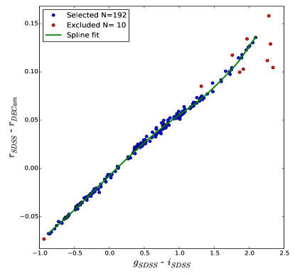
Figure 2.— Selected stars from the Next Generation Stellar Library in the $SDSS_{r}-DECam_{r}$ vs SDSS $g-i$ color plane. Sigma clipping selected (blue dots) and excluded (red) stars are shown. The spline fit is over-plotted as a green solid line.

The instrumental magnitudes of the $\omega$ Cen catalog are corrected for aperture by selecting a few bright isolated stars for each DECam ccd. The aperture correction is estimated accounting for chip to chip offsets and mapping the entire camera FoV. The best seeing image is selected as a reference for each filter, and the photometry of the other images is rescaled to this one, after bringing all the exposures to 1 second.

We then calibrated the mean instrumental magnitudes by following the equation:

$$M_{i}=m_{i}-K_{i}\times A_{i}+ZP_{i}$$ (1)

where $M_{i}$ and $m_{i}$ are the calibrated and instrumental magnitudes, respectively, $K_{i}$ are the extinction coefficients for the different filters, $A_{i}$ the air masses of the reference observations and $ZP_{i}$ the zero points. We used the extinction coefficients obtained by the DECam Legacy Survey (DECaLS) collaboration (Li et al., 2016) for the $g,r,i$ filters, namely $K_{g}$ = 0.18, $K_{r}$ = 0.0875 and $K_{i}$ = 0.065. For the $u$ filter we used the value $K_{u}$ = 0.40 obtained from DECam multiple $u-$band observations of the Galactic bulge. The air masses of the reference observations are $A_{u}=$1.19, $A_{g}=$1.15, $A_{r}=$1.19 and $A_{i}=$1.19. As ZPs we used the average of the ZPs derived by using the PS1 and SDSS photometry, namely $ZP_{u}=-$7.58, $ZP_{g}=-$5.48, $ZP_{r}=-$5.35 and $ZP_{i}=-$5.45.

The accuracy of the calibration is better than 2% for the $gri$ filters, while is $\approx$ 5% for the $u$ filter.

The calibrated photometric catalog for $\omega$ Cen  includes $686,746$ stars with a measurement in the $r$ and $i$ filters, $598,429$ with a measurement in the $g$ filter, and $398,604$ stars were also measured in the $u$ filter. Fig. 3 shows the $i,\ u-i$ (left panel), $i,\ g-i$ (middle) and $i,\ r-i$ (right) color-magnitude diagrams (CMDs) for all stars observed in the FoV towards $\omega$ Cen. The Signal to Noise ratio (S/N) is $\geq$ 20 down to $u\approx$ 23 mag, $g\approx$ 23 mag, $r\approx$ 23 mag, and $i\approx$ 22.5 mag, which are the catalog limiting magnitudes. These CMDs are heavily contaminated by field stars, mostly thin and thick disk and halo stars (see the Galactic simulation for a 1 deg² FoV around $\omega$ Cen  of Marconi et al. 2014 and their Figure 11).

The ACS photometry was kept in the VEGA system and we applied the camera charge transfer efficiency correction and the available ZPs for the $F435W$, $F625W$, $F658N$ filters following the prescriptions by Sirianni et al. (2005). For more details on the photometric calibration of this catalog see CS07.

4. A clean sample of cluster stars

To separate field and cluster stars we adopted a similar approach as suggested by Di Cecco et al. (2015). To take advantage of the multi-band optical photometry available for globular clusters they estimated the cluster ridge lines using different CMDs based on the same magnitude ($r$) and different colors. To improve the precision of the cluster ridge lines the candidate cluster stars were selected according to their radial distance and to their photometric errors. Once the multiple ridge lines were estimated they generated a multi-dimensional CMD and the candidate cluster stars were selected using a variable $\sigma$-clipping over the entire magnitude range. This approach is seen to be quite robust, since they were able to separate candidate field and cluster stars for M 71, a metal-rich globular projected onto the Galactic bulge.

However, the quoted method can be hardly adopted in a globular cluster like $\omega$ Cen, due to the presence of well-defined multiple sequences mainly caused by a difference in metal content (Calamida et al., 2009; Johnson & Pilachowski, 2010). Therefore, the separation was performed using a new improved approach. We estimated the ridge lines of the different sub-populations identified along the cluster red-giant branch (RGB), the main sequence turn-off (MSTO) and the main sequence (MS). The horizontal branch (HB) stars were not included since they are typically bluer than field stars. These ridge lines were estimated neglecting the stars located in the innermost cluster regions ($r\leq$ 3′) and applying several cuts in radial distance and in photometric accuracy. Note that to fully exploit the current photometric catalog we only selected stars with accurate measurements in all the four $ugri$ bands. Once the ridge lines (seven) have been estimated we performed a linear interpolation among them and generated a continuos multi-dimensional surface. Finally, we used two different statistical parameters to separate field and cluster stars:

1) we estimated the cumulative standard deviation among the position of individual stars and the reference surface;

2) we associated a figure of merit to the distance in magnitude and colors among the individual stars and the reference surface.

We have performed a number of test and trials to sharpen the selection criteria to separate cluster and field stars. The approach was conservative, in the sense that we preferred to possibly lose some of the candidate cluster stars instead of including possible candidate field stars. A glance at Fig. 4 shows the advantages of the current approach. The left panel displays the color-color-magnitude diagram, $u-r$ vs $g-i$ vs $r$, for candidate field (gray dots) and cluster (multi-color) stars seen from the front, while the right panel shows the same plot but seen from the back. Note that the candidate field stars display a smooth distribution both in magnitude and in color. In passing we note that the current approach can be applied to separate field and cluster stars thanks to the opportunity to use the $u$ filter, since this band allows a better sensitivity to both effective temperature and metallicity. Fig. 5 shows the candidate field stars in the $i,\ u-r$ CMD. No clear cluster sequence is present in the field star sample in the entire magnitude range down to $i\approx$ 23 mag. It is interesting to note the sequence of disk white dwarfs at -0.5$\leq u-r\leq$ 1.0 mag and $i\geq$ 18 mag that were excluded from the cluster sample after applying our selection method.

Table 1Positional, photometric and structural parameters of the Galactic Globular Cluster $\omega$ Cen 

Parameter		Ref.
$\alpha$ (J2000)	201.694625	1
$\delta$ (J2000)	-47.48330	1
$M_{V}$ (mag)	-10.3	3
$r_{c}$ (arcmin)	2.58	3
$r_{t}$ (arcmin)	57.03	2
$e$	0.12	4
$\sigma_{V}$ (km s-1)	$17\pm 1.6$	5
E(B-V)	$0.11\pm 0.02$	6
$(m-M)_{0}$ (mag)	$13.71\pm 0.02\pm 0.03$	1

Table 2Log of the observations collected with DECam on the 4m Blanco telescope for $\omega$ Cen (CTIO, NOAO, proposal IDs: 2014A-0327, 2015A-0151, 2016A-0189, PIs: A. Calamida, A. Rest).

Name	Exposure time	Filter	RA	DEC	Seeing
	(s)		(hh:mm:ss.s)	(dd:mm:ss.s)	(arcsec)
February 24, 2014
omegacen.u.ut140224.052814.fits	120	u	13:26:47.288	-47:28:45.894	1.2
omegacen.u.ut140224.053340.fits	120	u	13:27:00.889	-47:33:26.593	1.3
omegacen.u.ut140224.053907.fits	120	u	13:26:33.338	-47:31:08.396	1.2
omegacen.u.ut140224.054435.fits	120	u	13:26:13.607	-47:34:28.294	1.6
June 22, 2015
omegacen.g.ut150622.035733.fits	250	g	13:26:47.047	-47:28:45.995	1.2
omegacen.g.ut150622.040213.fits	250	g	13:26:27.319	-47:28:46.196	1.2
omegacen.g.ut150622.040649.fits	250	g	13:26:27.337	-47:32:06.295	1.2
omegacen.g.ut150622.041130.fits	250	g	13:26:47.058	-47:32:06.194	1.1
March 4, 2016
omegacen.r.ut160304.072010.fits	80	r	13:26:48.138	-47:27:41.994	0.8
omegacen.r.ut160304.072202.fits	80	r	13:26:40.258	-47:27:41.695	0.8
omegacen.r.ut160304.072350.fits	80	r	13:26:40.229	-47:26:21.494	0.8
omegacen.r.ut160304.072538.fits	80	r	13:26:48.178	-47:26:21.793	0.8

• This table is available in its entirety in a machine-readable form in the online journal.

Table 3Zero points derived for Stripe 82 field SDSS1048p0000 by using SDSS and PS1 photometry.

System	$u$	$g$	$r$	$i$	$rms_{u}$	$rms_{g}$	$rms_{r}$	$rms_{i}$
PS1	…	-5.466$\pm$0.002	-5.350$\pm$0.002	-5.440$\pm$0.002	…	0.03	0.02	0.03
SDSS	- 7.577$\pm$0.007	-5.495$\pm$0.003	-5.352$\pm$0.003	-5.462$\pm$0.002	0.05	0.04	0.03	0.03

Table 4Values of the peaks and Full-Width half maximum (FW) for the three Gaussians that fit the three sub-populations along $\omega$ Cen MS: P₁ for the red MS, P₂ for the MS-a and P₃ for the blue MS. See text for more details.

$\Delta$ Mag	P1	FW1	P2	FW2	P3	FW3
5’ $\leq r<$ 10’
18 $\leq i<$ 18.5	0.00	0.07	0.04	0.16	…	…
18.5 $\leq i<$ 19	0.00	0.09	0.04	0.21	…	…
19 $\leq i<$ 19.5	0.00	0.12	0.04	0.26	…	…
19.5 $\leq i<$ 20	0.00	0.12	0.03	0.30	-0.10	0.05
20 $\leq i<$ 20.5	0.00	0.19	0.19	0.19	-0.10	0.26
20.5 $\leq i<$ 21	0.01	0. 21	0.20	0.09	-0.18	0.16
10’ $\leq r<$ 15’
18 $\leq i<$ 18.5	0.00	0.04	0.03	0.11	…	…
18.5 $\leq i<$ 19	0.00	0.05	0.02	0.13	…	…
19 $\leq i<$ 19.5	0.00	0.06	0.03	0.19	-0.07	0.03
19.5 $\leq i<$ 20	0.00	0.09	0.01	0.20	-0.09	0.06
20 $\leq i<$ 20.5	0.00	0.09	0.01	0.28	-0.12	0.07
20.5 $\leq i<$ 21	0.00	0.09	-0.02	0.27	-0.15	0.07
15’ $\leq r<$ 66’
18 $\leq i<$ 18.5	0.00	0.05	0.06	0.07	…	…
18.5 $\leq i<$ 19	0.00	0.07	0.06	0.16	…	…
19 $\leq i<$ 19.5	0.00	0.07	0.08	0.09	-0.07	0.05
19.5 $\leq i<$ 20	0.00	0.05	0.03	0.09	-0.08	0.09
20 $\leq i<$ 20.5	0.00	0.07	0.04	0.16	-0.11	0.09
20.5 $\leq i<$ 21	0.00	0.09	0.06	0.16	-0.13	0.14

5. The cluster color-magnitude diagrams

Following the procedure described in section §4 we ended up with a catalog of 266,769 cluster members with a measurement in all the four $ugri$ filters. The $u$-band photometry is limiting the depth of the catalog, but it was essential in allowing the cluster and field star separation. Fig. 6 shows the same CMDs of Fig. 3 but for cluster members only. No selection in photometric accuracy is applied. All the cluster sequences are well-defined, including the extreme horizontal branch (EHB) at $u-i\approx$ -1, $g-i\approx$ -0.7, $r-i\approx$ -0.3 and 18 $<i<$ 20 mag, and the white dwarf (WD) cooling sequence at $u-i\approx$ -1, $g-i\approx$ -0.7, $r-i\approx$ -0.3 and $i<$ 21 mag. The CMDs reach $i\approx$ 21.5 mag with $S/N>$ 50.

To verify the plausibility of the photometric calibration we used theoretical isochrones and Zero Age Horizontal Branch (ZAHB) loci from the BASTI database. These models are in the Sloan photometric system (Fukugita et al., 1996) and were transformed to the DECam system by using the empirical transformations derived in section §3. Extinction coefficients in the $ugri$ filters were estimated by using the Cardelli et al. (1989) reddening law and DECam filter transmission functions. We obtained $A_{u}$ = 1.70$\times A_{V}$, $A_{g}$ = 1.18$\times A_{V}$, $A_{r}$ = 0.84$\times A_{V}$, and $A_{i}$ = 0.63$\times A_{V}$. We used an absolute distance modulus of $\mu_{0}$ = 13.71$\pm$0.02$\pm$0.03 mag (Braga et al., 2016) and a reddening of $E(B-V)$ = 0.11 $\pm$0.02 mag (Calamida et al., 2005). We selected two isochrones for the same age, $t$ = 12 Gyr, and different metallicities, namely $Z$ = 0.004, $Y$ = 0.251, and $Z$ = 0.0006, $Y$ = 0.246. These values, -1.84 $\leq[Fe/H]\leq$ -1.01, approximately bracket the bulk of $\omega$ Cen metallicity dispersion (Calamida et al., 2009). The agreement between theory and observations is quite good in the entire magnitude range in all the three CMDs. The HB in the $i,\ u-i$ CMD is slightly bluer than the ZAHBs. This effect might be due to the calibration uncertainties, $\approx$ 5%, and to uncertainties in the $u$-band bolometric correction of the models.

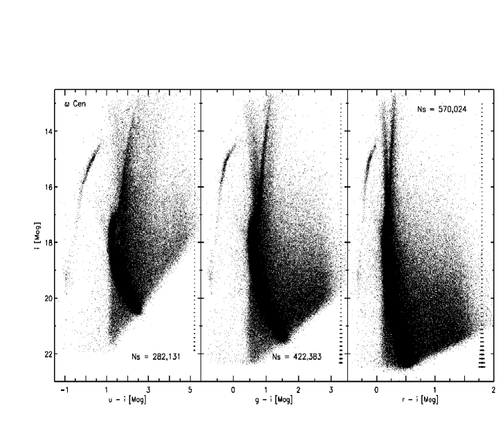
Figure 3.— DECam ugri color-magnitude diagrams towards $\omega$ Cen. Error bars are marked.

6. Astrometry and coordinate system

The astrometric calibration of $\omega$ Cen DECam catalog to the equatorial system J2000 was performed by using Photpipe and the Two Micron All Sky Survey (Cutri et al., 2003) catalog of stars as a reference. The final accuracy is better than 0.03” in both right ascension and declination.

The astrometry of the ACS catalog was performed by matching the photometry with stars from the catalog of van Leeuwen et al. (2000) with proper motions and membership probabilities (for more details see CS07).

We matched the ACS and DECam photometric catalogs for cluster members by using a 0.5” searching radius. The matched catalog includes 1,722,810 stars covering a FoV of 2.3$\times$2.2^∘ across $\omega$ Cen and including photometry in seven photometric bands, namely $F475W,F625W,F658N,u,g,r,i$ (see Fig. 1). To our knowledge, this is the largest multi-band data set ever collected for a Galactic globular cluster after our ACS-WFI catalog published in CS07.

The equatorial coordinates $\alpha$ and $\delta$ in degrees were converted to cartesian coordinates by following the prescriptions of van de Ven et al. (2006) with the cluster center at $\alpha_{0}$ = 201.694625^∘and $\delta_{0}$ = -47.48330^∘(Braga et al., 2016). Setting $x$ in the direction of West and $y$ in the direction of North:

$x=-r_{0}\cdot cos\delta\cdot sin\Delta\alpha$

$y=r_{0}\cdot(sin\delta\cdot cos\delta_{0}-cos\delta\cdot sin\delta_{0}\cdot cos\Delta\alpha)$

where $\Delta\alpha=\alpha-\alpha_{0}$ and $r_{0}=10,800/\pi$ to have $x$ and $y$ in arcminutes.

We then projected the cartesian coordinates $x$ and $y$ with the $x$ and $y$ axes aligned with the observed major and minor axes of $\omega$ Cen, respectively. To accomplish this we rotated the coordinates by the position angle of the cluster, defined as the angle between the major axis and the North direction measured counterclockwise by using a value of 100^∘ (van de Ven et al., 2006). The combined ACS-DECam photometric catalog with coordinates aligned on $\omega$ Cen major and minor axis will allow us to investigate the behavior of the cluster different sub-populations as a function of distance from the center.

7. The main-sequence split

Based on HST photometry Anderson (2002) before, and later Bedin et al. (2004), revealed that $\omega$ Cen MS is bifurcating into two main components, the so called blue-MS (bMS) and the red-MS (rMS). The color difference between the two sequences changes with magnitude, and they are clearly separated in the magnitude interval 20.5 $<V<$ 22. The HST observations included a central field and a field located at $\approx$ 17′  from the cluster center. A spectroscopic follow-up by Piotto et al. (2005) found that bMS stars are more metal-rich than rMS stars counter to expectations. These authors proposed that bMS stars constitute a helium-enhanced sub-population in the cluster to explain the observed anomaly. $\omega$ Cen MS split was also found by Sollima et al. (2007b) based on VLT photometry. They showed that the two sequences are still well-separated at $\approx$ 26′  from the cluster center and that bMS stars are more centrally concentrated compared to rMS stars. The ratio of bMS and rMS stars decreases from a value of $\approx$ 0.28 at a distance from the cluster center of $\approx$ 7′  down to 0.15 for distances larger than 19′. Bellini et al. (2010), by using deep HST observations collected in different filters from the ultraviolet to the red, showed the presence of a third MS, named MS-a, that better separates in the $F435W,\ F336W-F435W$ CMD, and seems to be connected to $\omega$ Cen faintest sub-giant branch (SGB), the so called SGB-a (Ferraro et al., 2004), and the reddest and most metal-rich RGB, the so-called RGB-a Pancino et al. (2000), and named $\omega$3 by us (CS07). However, these analyses were limited to the cluster central region (HST data) and up to a distance of 25′  (HST and VLT data). DECam photometry and the ability to remove the field component by using color-color-magnitude diagrams opens up the possibility to investigate the spatial distribution of the two MSs until $\omega$ Cen tidal radius.

The left panel of Fig. 7 shows a zoom of DECam $i,\ g-i$ CMD in the magnitude interval 18.0 $\leq i\leq$ 21.0. The split of the MS is evident, with the bMS well-separated from the rMS in the magnitude range 19.0 $\leq i\leq$ 21.0. This is the first time that $\omega$ Cen MS split is observed with a 4m-class ground-based telescope. The $g-i$ color distance between the two sequences is changing with magnitude and reaches a maximum of $\approx$ -0.18 mag at $i\approx$ 21 mag. Unfortunately, our catalog does not have the sufficient photometric accuracy to allow us to investigate the behavior of the MS at fainter magnitudes. The ridge line of the rMS is over-plotted on the $i,\ g-i$ CMD of Fig. 7 as a red solid line. The ridge line color at the corresponding magnitude was subtracted to each star observed color to straighten the MS. The result of this process is shown in the right panel of the figure. We then estimated the distance of each star from the cluster center by using the coordinates aligned with the major and minor axes and divided the stars in three concentric annuli from 5 to 66′, including approximately the same number of stars per radial annulus. Stars were then divided in six 0.5 magnitude bins from $i$ = 18 down to $i$ = 21. Fig. 8 shows the star $g-i$ observed color minus the ridge line color histograms for the six magnitude intervals for the annulus in the distance interval 10 $<r<$ 15′. The panels show that the color distributions are asymmetric, being skewed towards the red in the entire magnitude range, and they separate in two main peaks starting at $i\approx$ 19 mag. The skewness is probably due to the presence of the third MS (MS-a), that the accuracy of the photometry and the $g-i$ color sensitivity does not allow us to separate it from the rMS, and to the presence of blends and unresolved binaries. We fitted the six histograms with three Gaussians reproducing the rMS ($P_{1}$), the MS-a ($P_{2}$) and the bMS ($P_{3}$), respectively. The three Gaussian functions used in the fit and their sum are shown in the figure as red (rMS), green (MS-a), blue (bMS) and black solid lines. The peaks and the Full-Width Half Maximum values of the Gaussians are indicated in the plots and listed in Table 4.

DECam photometry clearly shows that $\omega$ Cen MS split is present at all distances from the cluster center until the tidal radius. The $g-i$ color separation between the rMS ($P_{1}$) and the bMS ($P_{3}$) is the same, within the uncertainties, for the three different annuli, going from $0.07$ to $0.15$ mag for 10 $\leq r<$15′, according to the magnitude interval.

7.1. The ratio of blue and red main-sequence stars

To characterize the spatial distribution of $\omega$ Cen MS stars we computed the ratio of bMS and rMS stars, $r(bMS/rMS)=N(bMS)/N(rMS)$, as a function of the radial distance. To select the sample of bMS and rMS stars we first produced a 3D CMD for stars in the magnitude interval 19.25 $<i<$ 20.5, where the MS best separates. Fig. 9 shows the 3D CMD: color $g-i$, magnitude $i$, and luminosity function. To overcome subtle problems in constraining the position of the MS peaks caused by the binning of the data, we associated to each star a Gaussian kernel with a sigma equal to its intrinsic error in the $g-i$ color measurement. The green surface was computed by summing all the individual Gaussians over the entire color and magnitude range. A glance at the surface discloses two distinct backbones tracing the bMS and the rMS (blue and red solid lines, respectively). To further improve the identification of bMS and rMS stars, the blue and the red lines display the peaks of the two sequences, while the black solid line marks the valley between the two different sub-populations, i.e. the relative minimum between the two relative maxima.

The 3D CMD plotted in Fig. 9 clearly shows that the separation between bMS and rMS stars is far from being trivial, since the difference in color is magnitude dependent. Moreover, the MSs associated to the two sub-populations display, at fixed magnitude, different broadenings in color. To overcome thorny problems in the selection criteria adopted to identify bMS and rMS stars, we adopted an incremental approach. Firstly, we only selected stars that are located within $\pm$ 0.02 mag from the blue and the red backbone in the 19.25 $<i<$ 20.5 magnitude interval. This means we selected stars with a distance in $g-i$ color from the backbone of $\Delta=$ 0.04 mag. The adopted minimum color bin was driven by the typical color uncertainty in the selected magnitude range. We then repeated the same selection but increasing the distance in color from the backbone. Note that the bMS and the rMS samples never overlap, since the inner boundary is traced by the valley plotted in Fig. 9. To improve the statistics of the two samples, the range in color was increased up to 0.3 mag. We performed a number of tests and this color bin is a good compromise between the width in color of the bMS plus the rMS and the contamination of field stars. It is clear that with a wider bin in color, we mainly select stars that are located along the slopes either of the bMS or of the rMS backbone. As a whole we ended up with 28 bins in $g-i$ color ranging from 0.02 to 0.3 mag.

To validate the criteria adopted for the selection of bMS and rMS stars Fig. 10 shows the quoted selection in the $i,\ g-i$ CMD. The left panel shows the selection based on a $g-i$ color range $\Delta=$ 0.04 mag. Note that for this selection the blue and the red samples are approaching the valley in the bright regime, $i<$ 19.4 mag, but they are well separated in the faint regime. The middle panel shows an intermediate selection in which the two sub-populations already approached the valley over the entire magnitude range, while the right panel shows bMS and rMS stars selected by using a wider $g-i$ color range.

Fig. 11 shows the 3D plot of the ratio between bMS and rMS stars as a function of the radial distance and of the $g-i$ color range used in the selection for the entire sample of stars included in the 19.25 $<i<$ 20.5 magnitude interval (left panel), for only the candidate cluster stars (middle), and for only the candidate field stars (right). The different color selections were plotted with different arbitrary colors to highlight the difference when moving from narrower to wider color bins. Table 5 lists the number of bMS and rMS stars and their ratio for the samples of candidate cluster and field stars for $\Delta=$ 0.15 mag. The ratios plotted in the three different panels and listed in the table display several relevant features worth being discussed in more detail:

1) The ratio between bMS and rMS is far from being constant across the body of the cluster. It shows a well defined minimum, $r(bMS/rMS)=0.17\pm 0.005$, for radial distances of 20 $<r<$ 25′, in which the ratio decreases by almost a factor of two from the half-mass radius (5′), and then it starts to steadily increase. Note that all previous investigations concerning the radial trend of bMS and rMS stars reached a maximum distance of $\approx$ 25′  from the cluster center.

2) The population ratios display two relative maxima in approaching the cluster center and for radial distances of the order of 45–50′. These findings are independent of the $g-i$ color bin used to select the sample of bMS and rMS stars and indeed the radial trends are quite similar when moving from the narrower to the wider bin. Moreover, the current finding is also independent of the approach used to select candidate cluster and field stars. The population ratios are similar in the left panel of Fig. 11, where the ratio is the entire sample of stars, and in the middle panel, where it is based on only candidate cluster members.

3) Data plotted in the middle panel of Fig. 11 further support the evidence that the maximum in the population ratio is attained in the outskirts of $\omega$ Cen ($r\approx$ 48′), where bMS stars are overwhelming rMS stars, the ratio being of the order of 1.2 (see Table 5). The population ratio increase in the innermost cluster regions only produces a relative maximum. This trend becomes, for statistical reasons, more clear when moving from the narrower to the wider color bins.

4) The radial trends of the population ratio display a steady decrease when moving from the maximum ($r\approx$ 48′) to the truncation radius ($r\approx$ 57′) of the cluster. This decrease is affected by statistics, and indeed, the narrower color bins are slightly noisier when compared to the wider ones.

The population ratios based on only candidate field stars plotted in the right panel of Fig. 11 show a trend that at glance might appear counterintuitive, since they display a well defined maximum in approaching the innermost cluster regions, with $r(bMS/rMS)=4.04\pm 0.15$. The expected trend would have been a relatively flat distribution, as observed for distances larger than $\approx$ 35′. However, this is a consequence of the fact that we are plotting the ratio between bMS and rMS stars and not the star counts. The ratios attain similar values, but the number of bMS and rMS stars among candidate cluster and field stars are significantly different. In passing we also note that the ripples showed by the cumulative population ratios are a consequence of small fluctuations in the number of blue and red candidate field stars.

To further quantify the difference in star counts between cluster and field candidate stars the left panel of Fig. 12 shows the ratio of blue candidate field and cluster stars. The radial trends show that star counts of blue field stars are at least two order of magnitude smaller than those of blue cluster stars. This means that the maximum in the bMS and rMS star ratio in the right panel of Fig. 11 is caused by a non-perfect separation between candidate field and cluster stars. However, the star counts of blue field stars are at most a few hundredths of the candidate blue cluster members. This means that they do not affect the current findings concerning the radial trend of the population ratio. The same outcome applies to the minimum and to the maximum of the population ratios. The candidate cluster bMS stars outnumber the candidate blue field stars up to radial distances of the order of 35′. In these regions the two samples attain, within the errors, star counts $log(N_{field}/N_{MS})\approx$ 0. At larger radial distances the candidate field stars outnumber, as expected, candidate cluster members. The ratios plotted in the right panel of Fig. 12 are based on candidate red field stars and candidate rMS stars. The radial trends are similar to the trends of the blue stars.

Data plotted in Fig. 12 are suggesting that we are quite confident concerning the robustness of the population ratios for radial distances smaller than $\approx$ 50′. The decrease in the population ratio at larger distances requires independent confirmation possibly based on photometric catalogs selected using proper motion.

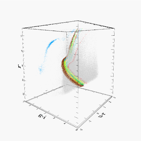
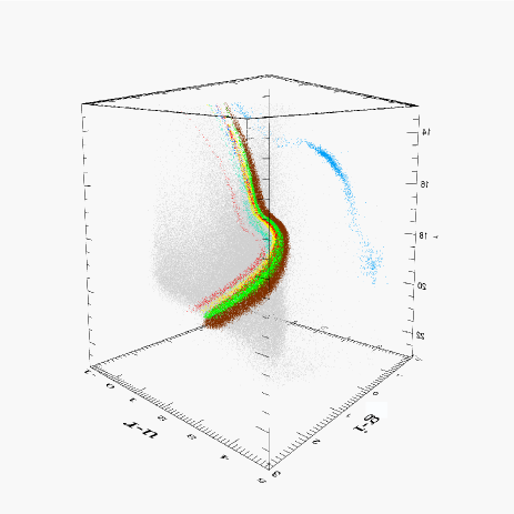
Figure 4.— ugri DECam color-color-magnitude diagram of $\omega$ Cen members (different colors mark different selected cluster sequences) and field stars (gray dots) seen from the front (top panel) and the back (bottom).

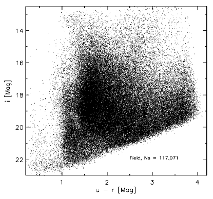
Figure 5.— DECam $i,\ u-r$ color-magnitude diagram of candidate field stars in the observed field of view.

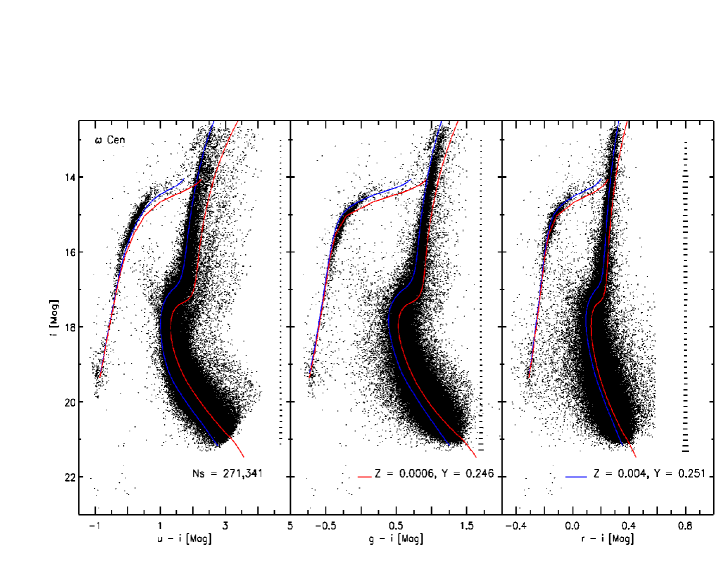
Figure 6.— DECam ugri color-magnitude diagrams of $\omega$ Cen cluster members. Isochrones for the same age, $t$ = 12 Gyr, and different metallicities are over-plotted (see labeled values). The respective zero age horizontal branch (ZAHB) tracks are also shown. Error bars are marked.

To further support our result we plotted in Fig. 13 the $i,\ g-i$ CMDs of candidate cluster (left panels) and field (right) stars for two external radial annuli, 30 $\leq r<$ 35 and 35 $\leq r<$ 60′, respectively. The figure shows that our method to separate cluster and field stars is very effective until large distances, $r\geq$ 30′, from the cluster center. However, as discussed before and illustrated in the previous figures, some $\omega$ Cen stars might be miss-classified as field stars in the more internal regions of the cluster. A residual contamination of field stars in the cluster MS samples might also be present at large distances from the center (see bottom left panel).

7.2. Star counts across the body of the cluster

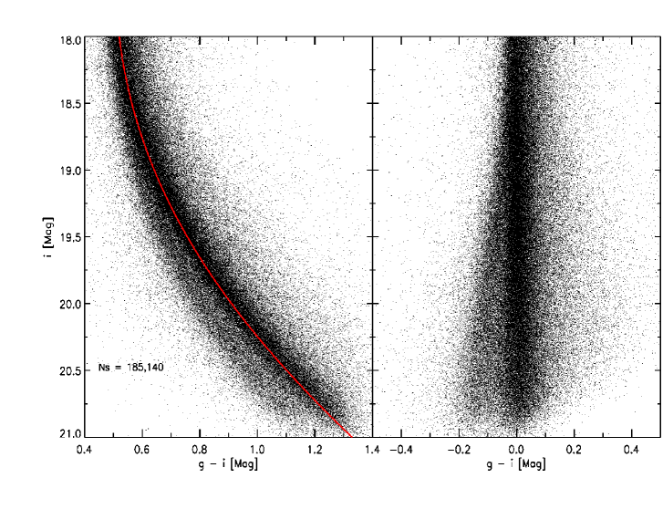
Figure 7.— Left - Zoom of the $\omega$ Cen $i,\ g-i$ color-magnitude diagram. The ridge line for the rMS is over-plotted as a red solid line. Error bars are marked. Right - Observed star $g-i$ color minus the ridge line color for the respective $i$ magnitude.

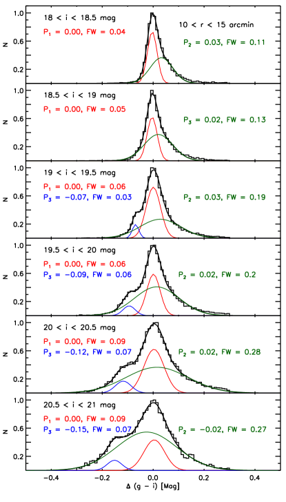
Figure 8.— $g-i$ color histograms of $\omega$ Cen straightened main-sequence for six $i$-band magnitude intervals for the distance annulus 10 $<r<$ 15′. The three Gaussian functions and their sum used to fit the histograms are indicated as red (rMS), green (MS-a), blue (bMS) and black (total) solid lines. The Peak (P) and Full-Width Half Maximum (FW) values for the Gaussians are shown.

The spatial distribution of $\omega$ Cen MS stars appears to be even more complicated than suggested by the radial gradient. The density map of the ratio between bMS and rMS stars is plotted in the left panel of Fig. 14. The population ratio shows a clumpy distribution, with a well-defined North/South asymmetry in the outermost cluster regions, being the bMS stars significantly more abundant in the Northern quadrants. Thus suggesting that the clumping in the radial gradient might be associated to azimuthal variations across the body of the cluster. It is worth noting that the main over-density of bMS stars is pointing towards the Galactic center (GC) (Dauphole et al., 1996; Leon et al., 2000, see the arrows plotted in the left panel of Fig. 14). These findings seem to suggest a connection between the spatial distribution of bMS stars and $\omega$ Cen dynamical evolution. A more quantitative analysis of the difference between bMS and rMS stars in these cluster regions does require new kinematic and spectroscopic data.

The anonymous referee suggested us to investigate whether possible extinction variations across the body of the cluster could affect the current population ratio. To verify that our result is not affected by foreground reddening, we downloaded reddening values provided by Schlafly & Finkbeiner (2011) for the region covered by the current photometric catalog. The reddening color density map of the observed field is shown in the right panel of Fig. 14. The reddening in the current FoV has a minimum value of $\approx$ 0.07 mag and a maximum of $\approx$ 0.18, with a mean reddening of $E(B-V)=$ 0.11 mag and a total dispersion of $\sigma_{E(B-V)}$= 0.02 mag. These values are in very good agreement with the dispersion $\sigma_{E(B-V)}\lesssim$ 0.03 mag found by Cannon & Stobie (1973) and Calamida et al. (2005) based on photometric studies of $\omega$ Cen. This low differential reddening could move stars from the blue to the red MS sample. However, the observed over-densities of bMS stars when moving towards the outermost cluster regions cannot be caused by an increase in the extinction. An increase in differential reddening causes a decrease in the population ratio, since truly bMS stars are moved into the rMS sample. Therefore, the current population ratio can be considered as a lower limit to the real one.

On the other hand, the presence of higher dust extinction ($E(B-V)\approx$ 0.15–0.16 mag) in the South-West corner of the cluster might explain the observed increase in rMS stars in the cluster regions located along the direction of $\omega$ Cen proper motion.

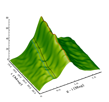
Figure 9.— 3D $i,\ g-i$ CMD of $\omega$ Cen main-sequence in the magnitude interval 19.25 $<i<$ 20.5. The vertical axis indicates the luminosity function as described in §7.1. The blue and red solid lines indicate the blue and the red main-sequence ridge lines, respectively. The black solid lines marks the valley, i.e. the relative minimum between the two relative maxima.

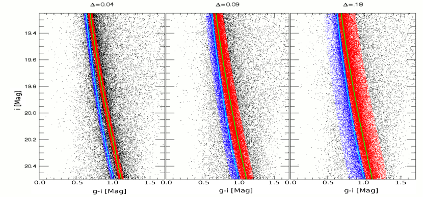
Figure 10.— $i,\ g-i$ CMDs of $\omega$ Cen main-sequence in the magnitude interval 19.25 $<i<$ 20.5. The three panels show blue (blue dots) and red (red) main-sequence stars selected by using different $g-i$ color limits, $\Delta$, indicated at the top of each panel. The cyan and green solid lines mark the blue and red main-sequence ridge lines, respectively. See the detailed explanation in §7.1.

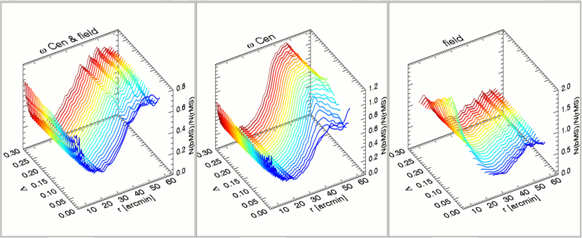
Figure 11.— Ratio of bMS and rMS stars as a function of distance from the cluster center and $g-i$ color bins used to select the stars, $\Delta$. The three panels show the same ratio for all the stars (left), for only candidate cluster members (middle) and for only candidate field members (right) in the magnitude interval 19.25 $<i<$ 20.5.

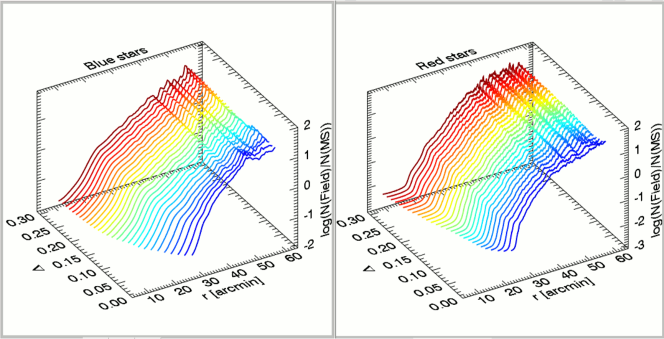
Figure 12.— Logarithm of the ratio of candidate field and cluster blue (left panel) and red (right) main-sequence stars in the magnitude interval 19.25 $<i<$ 20.5 for different $g-i$ color bins used to select the stars, $\Delta$.

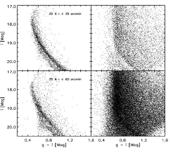
Figure 13.— $i,\ g-i$ CMDs of candidate cluster (left panels) and field (right panels) stars for two different external radial bins.

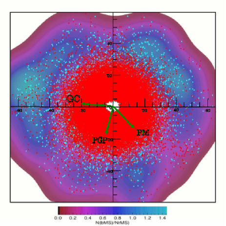
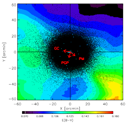
Figure 14.— Left - Density color map of the ratio of bMS and rMS stars as a function of star position in arcminutes. The green arrows mark the direction of the Galactic center (GC), $\omega$ Cen proper motion (PM), and the direction perpendicular to the Galactic center (PGP). The color scale is shown at the bottom. Right - Reddening color density map for the observed region across $\omega$ Cen as a function of star position in arcminutes. The direction of the GC, the cluster PM and the PGP are indicated with red arrows and the color scale is shown at the bottom.

7.3. Comparison with literature

Our result is in agreement with the findings of Bellini et al. (2009, hereinafter BE09), based on HST data, for distances 5 $\lesssim r\lesssim$ 10′. At larger distances and up to $r\approx$ 20′, i.e. the region of $\omega$ Cen sampled by Bellini et al., our ratio of bMS and rMS stars is significantly lower than the ratio found by the quoted authors. At $r\approx$ 15′, for instance, Bellini et al. found a ratio of 0.36$\pm$0.04, while we find a ratio of 0.21$\pm$0.003, more than 3$\sigma$ smaller. On the other hand, our findings do not agree with the study of Sollima et al. (2007b) for distances smaller than $r\approx$ 10′, while they agree very well at larger distances and up to $r\approx$ 25′, i.e., the cluster region sampled by VLT photometry. BE09 claim that Sollima et al. ratio is lower compared to their findings due to the wider color range they used to select rMS stars, which would include unresolved binaries and members of the third MS, making the bMS and rMS population ratio smaller. The different approaches used to select bMS and rMS stars might also be the origin of the difference we find between our ratios and Sollima et al. ratios at small distances from the cluster center.

As far as the difference between our ratios and BE09 values for distances larger than 10′, we have to take into account several circumstantial evidence. Our sample of rMS stars is contaminated by unresolved binaries, MS-a stars, and marginally by blends in these more external cluster regions. Photometric and spectroscopic analysis provide a binary frequency for $\omega$ Cen of $\approx$ 5% (Mayor et al., 1996; Sollima et al., 2007a), and MS-a stars, which are the counterpart of RGB-a stars, are less than 5% of cluster stars (Pancino et al., 2000, CS07). These factors will cause an artificial increase in the star counts of the rMS, i.e. a decrease in the population ratio we are dealing with. By accounting for these factors, our population ratio would agree with the findings of BE09. However, these factors cannot explain the global decreasing trend of the ratio of bMS and rMS stars observed with DECam data and not found by BE09. The number of binaries is indeed expected to decrease at increasing distances from the cluster center, and the MS-a stars are supposed to be more centrally concentrated compared to metal-poor stars (Pancino et al., 2003; Bellini et al., 2009). The number of these objects and blends decreases at larger distances from the cluster center, with the net effect of an increase of the bMS and rMS ratio. However, DECam data are clearly showing that this population ratio is decreasing from $\approx$7′  up to a distance of $\approx$ 25′, where it attains a broad minimum value of $\approx$ 0.17.

We are thus left with the following evidence:

a) the current population ratio agrees well with star counts provided by BE09 in the innermost cluster regions (5 $\leq r\leq$ 10′) and attains a value $r(bMS/rMS)\approx$ 0.3–0.4;

b) the current star counts agree well with star counts provided by SO07 in the cluster regions located between 10 $\leq r\leq$ 25′, and show a decreasing population ratio from a value $r(bMS/rMS)\approx$ 0.3–0.4 down to $\approx$ 0.15–0.2.

c) $r(bMS/rMS)$ is increasing for distances larger than $\approx$ 25′  reaching a peak value of $\approx$ 1.2 at $\approx$ 48′

The above empirical evidence brings forward a very interesting implication. Spectroscopic measurements are available for 17 blue MS stars and they suggest that the bMS is more metal-rich than the rMS (Piotto et al., 2005). Our photometric analysis shows that the radial trend of this sub-population becomes more and more relevant when moving towards the outskirts of the cluster. This behavior is different from what it is observed in some nearby dwarf galaxies, where more metal-rich stars are centrally concentrated when compared with the more metal-poor ones (Bono et al., 2010; Fabrizio et al., 2015). This radial trend is further supported by metallicity gradients based on spectroscopic measurements of nearby dwarf galaxies (Ho et al., 2015) and on photometric indices (Martínez-Vázquez et al., 2016), suggesting either a relatively flat metallicity distribution or a steady decrease when moving from the innermost to the outermost galaxy regions. $\omega$ Cen seems to show an opposite trend with a population of more metal-rich stars less concentrated compared to the more metal-poor population. The reasons for the possible difference in the metallicity trend between $\omega$ Cen and nearby dwarf galaxies are not clear and new spectroscopic measurements to infer kinematical and abundance properties of a larger sample of bMS and rMS stars at different radial distances are required to better characterize their nature or nurture.

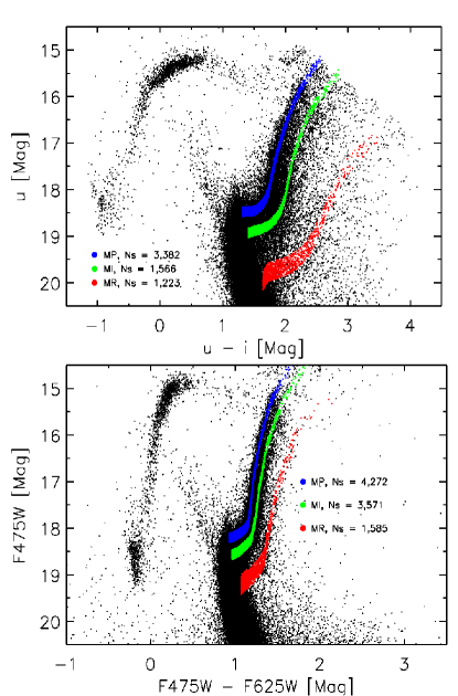
Figure 15.— Top - DECam $u,\ u-i$ CMD of $\omega$ Cen cluster members. The selected metal-poor (MP) red-giant branch stars (blue dots), metal-intermediate (MI, green), and metal-rich (MR, red) are over-plotted. Bottom: ACS $F475W,\ F475W-F625W$ CMD of $\omega$ Cen cluster members. Selected MP, MI and MR stars are marked.

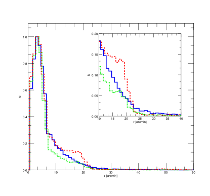
Figure 16.— Histograms of the spatial distribution of the metal-poor (blue solid line), metal-intermediate (green dotted-dashed), and metal-rich (red dashed) sub- and red-giant branch stars. The inset shows a zoom of the region included in 10 $<r<$ 40′.

8. The spatial distribution of red-giant branch stars

The bMS has its counterpart in one of the multiple RGBs of $\omega$ Cen, possibly at a metallicity intermediate for the cluster range (for more details on the correspondence between the triple MS and the multiple sub- and red-giant branches see Bellini et al. 2010). Unfortunately, it is not possible to clearly separate the different intermediate RGBs without using the information on the star chemical composition. For the more central regions of the cluster, up to $\approx$ 25′, low- and high-resolution spectroscopy and photometric metallicities are available. For the outskirts of the cluster, no metallicity information is available so far. Therefore, we decided to investigate the spatial distribution of the bluest and brightest SGB/RGB, the most MP sub-population in $\omega$ Cen according to spectroscopy, corresponding to the rMS. We compared the properties of this sub-population to the ones of the faintest and reddest SGB/RGB, the most MR cluster sub-population according to spectroscopic measurements and corresponding to the reddest MS. The reddest MS, or MS-a, is difficult to separate from the rMS because it overlaps with its sequence of unresolved binaries. However, MS-a has its continuation on $\omega$ Cen reddest RGB, the $\omega$3 branch, which constitutes the most MR sub-population of the cluster based on spectroscopic data (Pancino et al., 2000, 2007). The $\omega$3 branch is well-separated from the other RGBs in the $i,\ u-i$ or $u,\ u-i$ CMDs and the $F475W,\ F475W-F625W$ or $F625W,\ F475W-F625W$ CMDs, where the temperature sensitivity is larger (see Fig. 6). Therefore, we used the $u,\ u-i$ CMD, and for the internal regions of the cluster, $r\lesssim$ 5′, the $F475W,\ F475W-F625W$ CMD to select a sample of stars along the $\omega 3$ branch. We also decided to compare the properties of $\omega 3$ stars and of the most MP sub-population with a sample of stars representative of a cluster metal-intermediate (MI) sub-population. To select candidate MP and MI stars we used the following method. We draw two ridge lines following the MP and one MI RGB on the $u,\ u-i$ and $F475W,\ F475W-F625W$ CMD, respectively, and selected stars 0.1 mag fainter and brighter than these ridge lines. Note that the aim of this analysis is to select a sample of MP stars and of stars with a metallicity intermediate between the MP and the $\omega$3 sub-population.

Fig. 15 shows DECam $u,\ u-i$ (top panel) and ACS $F475W,\ F475W-F625W$ CMD (bottom) with the selected sample of MP (blue dots), MI (green) and MR (red) stars. The three samples of cluster stars have a similar completeness since both DECam and ACS photometric catalogs are complete down to the turn-off level. The total sample of MP stars includes $\approx$ 8,200 objects, while the MI and the MR one include $\approx$ 5,400 and $\approx$ 2,900, respectively. Note that we are interested in investigating the spatial distribution of these sub-populations and not in determining their absolute star counts and ratios.

Fig. 16 shows the histograms of the radial distance in arcminutes for the MP (solid blue line), the MI (dashed-dotted green) and the MR (dashed red) star samples. The spatial distributions of the MP and MR samples are very similar until $\approx$ 12′, while the fraction of MR stars increases for larger distances until $\approx$ 23′. The spatial distribution of the MI sample is different from either the MP and the MR spatial distributions starting from a distance of $\approx$ 8′  from the cluster center. The frequency of MI stars is lower compared to MP and MR stars, from this distance until the tidal radius. The inset of Fig. 16 shows a zoom of the radial distributions from 10 to 40′. It is clear how the number of MR stars increases compared to the MP ones starting at $\approx$ 12′  and then start decreasing again at $\approx$ 23′, while the number of MI stars is always lower in this distance range. For distances larger than $\approx$ 40′, statistics is preventing us to fully characterize the behavior of these sub-populations. To verify that our method to select the sample of MI red giants did not alter the analysis we performed the following test. We selected MI stars by moving the RGB ridge line 0.1 and 0.2 mag brighter and fainter on both the CMDs. We then compared the spatial distribution of the new sample of MI stars with those of the MP and MR stars. The result is the same within uncertainties, with the MI stars being more centrally concentrated compared to the MP and the MR stars.

Fig. 17 shows the cumulative radial distributions of MP, MI and MR stars. This plot clearly shows that MI stars are more centrally concentrated compared to the MP and the MR stars, while the MP stars are more concentrated than the MR stars for distances 10 $\lesssim r\lesssim$ 20′. Moreover, the $\omega 3$ sub-population has a more extended spatial distribution when considering distances larger than 10′. This result confirms the findings of CS07, where an increase of $\omega$3 star counts compared to the other RGs was observed with increasing distance from the cluster center. In particular, the fraction of $\omega$3 stars increases from $\approx$ 3% at $r\approx$ 8′  to $\approx$ 7% for larger distances (for more details please see their Table 3).

The current results also agree with previous findings by Hilker & Richtler (2000) based on Strömgren photometric metallicities for a sample of $\omega$ Cen RGs. These authors showed that more metal-rich RGs are more concentrated compared to more metal-poor stars within a radius of 10′  from the cluster center. Sollima et al. (2005), based on photometry of a sample of RGs for a field of view of $\approx$ 0.2$\times$0.2^∘ across the cluster, found a similar result. All these previous studies were based on photometric catalogs covering a radial distance until $\approx$ 20′. DECam data allowed us for the first time to analyze the spatial distribution of $\omega$ Cen RGB sub-populations across a much larger portion of the cluster and to disclose the peculiar behavior of $\omega 3$ branch stars.

We also investigated for the presence of a spatial segregation of the MP, MI and MR star sample. Table 6 lists the ratio of MR, MI and MP stars, $N(MR)/N(MP)$ and $N(MI)/N(MP)$, in the four quadrants of $\omega$ Cen, i.e. NW, NE, SW and SE. For the MR to MP star ratio, values are in agreement within uncertainties in the three NW, SW and NE quadrants, while a deficiency of MP stars is present in the SE quadrant. The MI to MP star ratio show a clear West-East asymmetry, due to the decrease of MP stars in the Southern quadrant of the cluster, while MI stars are more numerous in the NW, NE, and SE quadrants of $\omega$ Cen. The same table lists the number of MP, MI and MR stars in the four different regions. A clear asymmetry is present, with the MP being much more numerous in the two Northern quadrants, while MR and MI stars have a deficiency in the SW quadrant of $\omega$ Cen.

Jurcsik (1998) showed that more metal-rich stars in $\omega$ Cen ($[Fe/H]\geq-1.25$) are segregated in the Southern part of the cluster, while the metal-poor ($[Fe/H]\leq-1.75$) stars in the Northern. The centroid of these two groups are $\approx$ 6′  apart. The segregation of MR stars in the Southern half of $\omega$ Cen was confirmed by Hilker & Richtler (2000), while they did not find an equivalent segregation for the MP sub-population. Our data seem to support a different distribution of MP, MI and MR stars in $\omega$ Cen, and a clear excess of MP stars in the Northern half of the cluster and a deficiency of MI and MR stars in the SW quadrant. However, we do not have homogenous abundance measurements for MP, MI and MR stars up to $\omega$ Cen tidal radius. Spectroscopic measurements for stars belonging to the different sub-populations in the outskirts of the cluster are now needed to better characterize the spatial distribution of MP, MI and MR RGB stars in $\omega$ Cen.

Table 5Star counts and population ratio for bMS and rMS candidate $\omega$ Cen and field stars.

Distance	$N(rMS)$	$N(NbMS)$	$N(rMS)_{field}$	$N(bMS)_{field}$	$r(bMS/rMS)$	$r(bMs/rMs)_{field}$
(arcmin)
7.5	21128	7672	69	50	0.36$\pm$0.003	0.72$\pm$0.13
12.5	26778	6921	23	93	0.25$\pm$0.003	4.04$\pm$0.15
17.5	16271	3053	54	82	0.19$\pm$0.004	1.52$\pm$0.03
22.5	8051	1340	314	200	0.17$\pm$0.005	0.64$\pm$0.02
27.5	3360	717	663	270	0.21$\pm$0.009	0.41$\pm$0.01
32.5	1308	512	1171	384	0.39$\pm$0.02	0.33$\pm$0.01
37.5	470	334	1349	588	0.71$\pm$0.05	0.44$\pm$0.01
42.5	199	193	1401	708	0.97$\pm$0.10	0.50$\pm$0.01
47.5	115	143	1387	873	1.24$\pm$0.15	0.63$\pm$0.01
52.5	93	93	1383	915	1.00$\pm$0.15	0.66$\pm$0.01
57.5	78	59	1166	778	0.76$\pm$0.13	0.67$\pm$0.02

Table 6Number of metal-poor (MP) and metal-rich (MR) sub- and red-giant branch stars in the different quadrants of $\omega$ Cen.

	$N(MR)/N(MP)$	$N(MI)/N(MP)$	$N(MP)$	$N(MI)$	$N(MR)$
NW	0.34$\pm$0.02	0.57$\pm$0.02	2651$\pm$51	1504$\pm$39	829$\pm$29
SW	0.35$\pm$0.02	0.57$\pm$0.02	1837$\pm$43	1056$\pm$32	636$\pm$25
NE	0.38$\pm$0.02	0.72$\pm$0.02	1915$\pm$44	1377$\pm$37	761$\pm$28
SE	0.41$\pm$0.02	0.81$\pm$0.03	1616$\pm$40	1318$\pm$36	682$\pm$26

9. Summary and conclusions

We presented multi-band photometry of $\omega$ Cen for a total FoV of $\approx$ 2$\times$2^∘ across the cluster. Images were collected with the wide field camera DECam and combined with ACS data for the crowded regions of the cluster core. The availability of the $u$-band photometry allowed us to use a new method based on color-color-magnitude diagrams to separate cluster and field stars. We ended up with a final photometric catalog of $\approx$ 1.7 million cluster members, including photometry in seven filters, namely $F475W,F625W,F658N,u,g,r,i$. To our knowledge, this is the largest multi-band data set ever collected for a Galactic globular cluster and covering the widest FoV after our ACS-WFI catalog published in CS07.

DECam precise photometry allowed us to observe the split along $\omega$ Cen MS and to show that it is present at all distances from the cluster center. The bMS is well-separated from the rMS in the magnitude range 19.0 $\leq i\leq$ 21.0. The $g-i$ color distance between the two sequences is changing with magnitude and reaches a maximum of -0.18 mag at $i\approx$ 21 mag. The color separation between the rMS and the bMS is the same, within the uncertainties, at all distances from $\omega$ Cen center, ranging from $\approx$ 0.07 to $\approx$ 0.18 mag according to the magnitude interval.

DECam data allowed us for the first time to analyze the spatial distribution of the different $\omega$ Cen sub-populations across the cluster until the nominal tidal radius of 57′. In particular, we were able to investigate the spatial distribution of the two cluster main sequences. We found that stars belonging to the bMS are more centrally concentrated compared to stars belonging to the rMS up to a distance of $\approx$ 25′. The frequency of bMS stars is then steadily increasing up to $\approx$ 50′, with the ratio of bMS and rMS stars being larger than 1. The ratio of bMS to rMS stars shows an asymmetric clumpy distribution across the cluster, with an excess of bMS stars in the Northern half. The over-density of bMS stars in the cluster North-East quadrant is pointing towards the Galactic center, suggesting a connection between the spatial distribution of bMS stars and $\omega$ Cen dynamical evolution.

Unfortunately, our photometry does not allow us to identify the continuation of the bMS on the sub- and red-giant branch phases. We then analyzed the spatial distribution of a sample of MP and MI stars selected along the sub- and red-giant branch by using ridge lines in the $u,\ u-i$ and $F475W,\ F475W-F625W$ CMDs. Moreover, stars belonging to the $\omega$3 branch, the most MR sub-population in the cluster according to spectroscopy, were also selected. The three samples show a different spatial distribution; MI stars are more concentrated compared to MP and MR ones, while MP star are more concentrated than MR stars for distances in the interval 10 $\lesssim r\lesssim$ 20′. Data clearly show that the $\omega 3$ sub-population has a more extended spatial distribution when considering distances larger than 10′. This result confirms the findings of CS07, where an increase of the number of $\omega$3 stars compared to the other RGs with increasing distance from the cluster center was found. Star counts of the MP, MI and MR samples show that a deficiency of MI and MR stars the SW quadrant of $\omega$ Cen is present. Moreover, MP stars are more numerous in the Northern half of the cluster.

Stellar populations with different metallicities and age show different spatial distributions with the more metal-rich sub-populations being more centrally concentrated in some nearby dwarf spheroidal galaxies such as Carina, Sculptor, Fornax (Monelli et al., 2003; del Pino et al., 2013; Fabrizio et al., 2015; Ho et al., 2015; Martínez-Vázquez et al., 2016). The same behavior is observed in a Galactic globular cluster presenting a significant spread in iron abundance, Terzan 5. The metal-rich sub-population in this cluster is more centrally concentrated compared to the metal-poor one (Ferraro et al., 2016). The case of $\omega$ Cen seems to be different from both known Local Group dwarf spheroidal galaxies and clusters presenting stellar populations with different metallicities. $\omega$ Cen MI selected RGs are indeed more centrally concentrated compared to the MP ones, but the $\omega 3$ sub-population shows a more extended spatial distribution. The bMS stars, spectroscopically claimed to be more metal-rich compared to rMs stars, also show a more extended and very asymmetric spatial distribution. A few main conclusions can then be drawn:

• $\omega$ Cen hosts a metal-intermediate RGB sub-population that behaves as the metal-intermediate and metal-rich stellar populations in some nearby dwarf spheroidal galaxies and Terzan 5, being more centrally concentrated compared to the cluster metal-poor RGB sub-population. This stellar sub-population is peculiar compared to the typical second generation of stars present in other globular clusters, presenting not only a different iron abundance and its own chemical anti-correlations, according to spectroscopic analyses (Gratton et al., 2011; Marino et al., 2011, 2012), but also a very different spatial distribution;

• $\omega$ Cen bMS stars are more centrally concentrated compared to rMS stars up to a distance of $\approx$ 25′. The frequency of bMS stars, supposedly more metal-rich than the rMS stars according to spectroscopic measurements, steadily increases at larger distances, outnumbering the rMS stars until approximately the cluster tidal radius. Their spatial distribution is asymmetric and clumpy, with an excess of bMS stars in the direction of the Galactic center;

• $\omega$ Cen hosts a metal-rich sub-population making up the cluster third MS, MS-a, and the reddest and faintest RGB, the $\omega$3 branch. These stars are more centrally concentrated compared to more metal-poor stars up to a distance of $\approx$ 10′  from the cluster center, and their frequency increases at larger distances, showing a more extended spatial distribution;

• The behavior of the bMS and the $\omega$3 branch is similar, being both sub-populations more concentrated in the central regions and more extended in the outskirts of the cluster. This results suggests a possible common origin for these stellar sub-populations.

The current photometric catalog, thanks to its accuracy and spatial coverage, allowed us to disclose the complex spatial distribution of different stellar sub-populations in $\omega$ Cen. These results, if confirmed, will make $\omega$ Cen the only stellar system known to have more metal-rich stars with a more extended spatial distribution compared to more metal-poor stars.

Further data are now needed to solve the $\omega$ Cen puzzle. The current photometry combined with abundance and radial velocity measurements for stars of the different stellar sub-populations across the entire cluster will allow us to better understand the origin of $\omega$ Cen.

Further homogeneous photometric data are also needed to better characterize the behavior of the different stellar sub-populations until and beyond the nominal tidal radius of 57′. We have an approved DECam proposal to observe an area around $\omega$ Cen beyond its nominal tidal radius. The new data will allow us to better characterize the spatial distribution of $\omega$ Cen different stellar sub-populations. In particular, we are interested in confirming the more extended spatial distribution of the bMS and the $\omega$3 branch stars. With homogenous photometry covering a FoV of at least 3$\times$3^∘  across the cluster and including the $u$-filter, we will be also able to confirm the presence of stellar over-densities tracing tidal tails around $\omega$ Cen, previously found by Marconi et al. (2014), and to detect new stellar debris if present.

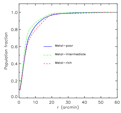
Figure 17.— Cumulative radial distributions of metal-poor (blue solid line), metal-intermediate (green dashed-dotted), and metal-rich (red dashed) sub- and red-giant branch stars.

References

- Anderson (2002) Anderson, J. 2002, in Astronomical Society of the Pacific Conference Series, Vol. 265, Omega Centauri, A Unique Window into Astrophysics, ed. F. van Leeuwen, J. D. Hughes, & G. Piotto, 87
- Bedin et al. (2004) Bedin, L. R., Piotto, G., Anderson, J., et al. 2004, ApJ, 605, L125
- Bellini et al. (2010) Bellini, A., Bedin, L. R., Piotto, G., et al. 2010, AJ, 140, 631
- Bellini et al. (2009) Bellini, A., Piotto, G., Bedin, L. R., et al. 2009, A&A, 507, 1393
- Bono et al. (2010) Bono, G., Stetson, P. B., Walker, A. R., et al. 2010, PASP, 122, 651
- Braga et al. (2016) Braga, V. F., Stetson, P. B., Bono, G., et al. 2016, AJ, 152, 170
- Calamida et al. (2009) Calamida, A., Bono, G., Stetson, P. B., et al. 2009, ApJ, 706, 1277
- Calamida et al. (2005) Calamida, A., Stetson, P. B., Bono, G., et al. 2005, ApJ, 634, L69
- Cannon & Stobie (1973) Cannon, R. D. & Stobie, R. S. 1973, MNRAS, 162, 207
- Cardelli et al. (1989) Cardelli, J. A., Clayton, G. C., & Mathis, J. S. 1989, ApJ, 345, 245
- Castellani et al. (2007) Castellani, V., Calamida, A., Bono, G., et al. 2007, ApJ, 663, 1021
- Cutri et al. (2003) Cutri, R. M., Skrutskie, M. F., van Dyk, S., et al. 2003, VizieR Online Data Catalog, 2246
- Dauphole et al. (1996) Dauphole, B., Geffert, M., Colin, J., et al. 1996, A&A, 313, 119
- del Pino et al. (2013) del Pino, A., Hidalgo, S. L., Aparicio, A., et al. 2013, MNRAS, 433, 1505
- Di Cecco et al. (2015) Di Cecco, A., Bono, G., Prada Moroni, P. G., et al. 2015, AJ, 150, 51
- Fabrizio et al. (2015) Fabrizio, M., Nonino, M., Bono, G., et al. 2015, A&A, 580, A18
- Ferraro et al. (2002) Ferraro, F. R., Bellazzini, M., & Pancino, E. 2002, ApJ, 573, L95
- Ferraro et al. (2016) Ferraro, F. R., Massari, D., Dalessandro, E., et al. 2016, ApJ, 828, 75
- Ferraro et al. (2004) Ferraro, F. R., Sollima, A., Pancino, E., et al. 2004, ApJ, 603, L81
- Fukugita et al. (1996) Fukugita, M., Ichikawa, T., Gunn, J. E., et al. 1996, AJ, 111, 1748
- Gratton et al. (2011) Gratton, R. G., Johnson, C. I., Lucatello, S., D’Orazi, V., & Pilachowski, C. 2011, A&A, 534, A72
- Hilker & Richtler (2000) Hilker, M. & Richtler, T. 2000, A&A, 362, 895
- Ho et al. (2015) Ho, N., Geha, M., Tollerud, E. J., et al. 2015, ApJ, 798, 77
- Johnson & Pilachowski (2010) Johnson, C. I. & Pilachowski, C. A. 2010, ApJ, 722, 1373
- Jurcsik (1998) Jurcsik, J. 1998, ApJ, 506, L113
- Kayser et al. (2006) Kayser, A., Hilker, M., Richtler, T., & Willemsen, P. G. 2006, A&A, 458, 777
- Leon et al. (2000) Leon, S., Meylan, G., & Combes, F. 2000, A&A, 359, 907
- Li et al. (2016) Li, T. S., DePoy, D. L., Marshall, J. L., et al. 2016, AJ, 151, 157
- Marconi et al. (2014) Marconi, M., Musella, I., Di Criscienzo, M., et al. 2014, MNRAS, 444, 3809
- Marino et al. (2012) Marino, A. F., Milone, A. P., Piotto, G., et al. 2012, ApJ, 746, 14
- Marino et al. (2011) Marino, A. F., Milone, A. P., Piotto, G., et al. 2011, ApJ, 731, 64
- Martínez-Vázquez et al. (2016) Martínez-Vázquez, C. E., Monelli, M., Gallart, C., et al. 2016, MNRAS, 461, L41
- Mayor et al. (1996) Mayor, M., Duquennoy, A., Udry, S., Andersen, J., & Nordstrom, B. 1996, in Astronomical Society of the Pacific Conference Series, Vol. 90, The Origins, Evolution, and Destinies of Binary Stars in Clusters, ed. E. F. Milone & J.-C. Mermilliod, 190
- Mayor et al. (1997) Mayor, M., Meylan, G., Udry, S., et al. 1997, AJ, 114, 1087
- Monelli et al. (2003) Monelli, M., Pulone, L., Corsi, C. E., et al. 2003, AJ, 126, 218
- Norris & Da Costa (1995) Norris, J. E. & Da Costa, G. S. 1995, ApJ, 447, 680
- Norris et al. (1997) Norris, J. E., Freeman, K. C., Mayor, M., & Seitzer, P. 1997, ApJ, 487, L187
- Norris et al. (1996) Norris, J. E., Freeman, K. C., & Mighell, K. J. 1996, ApJ, 462, 241
- Pancino et al. (2000) Pancino, E., Ferraro, F. R., Bellazzini, M., Piotto, G., & Zoccali, M. 2000, ApJ, 534, L83
- Pancino et al. (2007) Pancino, E., Galfo, A., Ferraro, F. R., & Bellazzini, M. 2007, ApJ, 661, L155
- Pancino et al. (2003) Pancino, E., Seleznev, A., Ferraro, F. R., Bellazzini, M., & Piotto, G. 2003, MNRAS, 345, 683
- Piotto et al. (2005) Piotto, G., Villanova, S., Bedin, L. R., et al. 2005, ApJ, 621, 777
- Rest et al. (2014) Rest, A., Scolnic, D., Foley, R. J., et al. 2014, ApJ, 795, 44
- Rest et al. (2005) Rest, A., Stubbs, C., Becker, A. C., et al. 2005, ApJ, 634, 1103
- Saha et al. (2010) Saha, A., Olszewski, E. W., Brondel, B., et al. 2010, AJ, 140, 1719
- Schechter et al. (1993) Schechter, P. L., Mateo, M., & Saha, A. 1993, PASP, 105, 1342
- Schlafly & Finkbeiner (2011) Schlafly, E. F. & Finkbeiner, D. P. 2011, ApJ, 737, 103
- Scolnic et al. (2015) Scolnic, D., Casertano, S., Riess, A., et al. 2015, ApJ, 815, 117
- Sirianni et al. (2005) Sirianni, M., Jee, M. J., Benítez, N., et al. 2005, PASP, 117, 1049
- Sollima et al. (2009) Sollima, A., Bellazzini, M., Smart, R. L., et al. 2009, MNRAS, 396, 2183
- Sollima et al. (2007a) Sollima, A., Ferraro, F. R., & Bellazzini, M. 2007a, MNRAS, 381, 1575
- Sollima et al. (2007b) Sollima, A., Ferraro, F. R., Bellazzini, M., et al. 2007b, ApJ, 654, 915
- Sollima et al. (2005) Sollima, A., Ferraro, F. R., Pancino, E., & Bellazzini, M. 2005, MNRAS, 357, 265
- Suntzeff & Kraft (1996) Suntzeff, N. B. & Kraft, R. P. 1996, AJ, 111, 1913
- van de Ven et al. (2006) van de Ven, G., van den Bosch, R. C. E., Verolme, E. K., & de Zeeuw, P. T. 2006, A&A, 445, 513
- van Leeuwen et al. (2000) van Leeuwen, F., Le Poole, R. S., Reijns, R. A., Freeman, K. C., & de Zeeuw, P. T. 2000, A&A, 360, 472
- Villanova et al. (2007) Villanova, S., Piotto, G., King, I. R., et al. 2007, ApJ, 663, 296