Adversarial Attacks on Neural Network Policies
Abstract
Machine learning classifiers are known to be vulnerable to inputs maliciously constructed by adversaries to force misclassification. Such adversarial examples have been extensively studied in the context of computer vision applications. In this work, we show adversarial attacks are also effective when targeting neural network policies in reinforcement learning. Specifically, we show existing adversarial example crafting techniques can be used to significantly degrade test-time performance of trained policies. Our threat model considers adversaries capable of introducing small perturbations to the raw input of the policy. We characterize the degree of vulnerability across tasks and training algorithms, for a subclass of adversarial-example attacks in white-box and black-box settings. Regardless of the learned task or training algorithm, we observe a significant drop in performance, even with small adversarial perturbations that do not interfere with human perception. Videos are available at http://rll.berkeley.edu/adversarial.
1 Introduction
Recent advances in deep learning and deep reinforcement learning (RL) have made it possible to learn end-to-end policies that map directly from raw inputs (e.g., images) to a distribution over actions to take. Deep RL algorithms have trained policies that achieve superhuman performance on Atari games [15, 19, 16] and Go [21], perform complex robotic manipulation skills [13], learn locomotion tasks [19, 14], and drive in the real world [7].
These policies are parametrized by neural networks, which have been shown to be vulnerable to adversarial attacks in supervised learning settings. For example, for convolutional neural networks trained to classify images, perturbations added to the input image can cause the network to classify the adversarial image incorrectly, while the two images remain essentially indistinguishable to humans [22]. In this work, we investigate whether such adversarial examples affect neural network policies, which are trained with deep RL. We consider a fully trained policy at test time, and allow the adversary to make limited changes to the raw input perceived from the environment before it is passed to the policy.
Unlike supervised learning applications, where a fixed dataset of training examples is processed during learning, in reinforcement learning these examples are gathered throughout the training process. In other words, the algorithm used to train a policy, and even the random initialization of the policy network’s weights, affects the states and actions encountered during training. Policies trained to do the same task could conceivably be significantly different (e.g., in terms of the high-level features they extract from the raw input), depending on how they were initialized and trained. Thus, particular learning algorithms may result in policies more resistant to adversarial attacks. One could also imagine that the differences between supervised learning and reinforcement learning might prevent an adversary from mounting a successful attack in the black-box scenario, where the attacker does not have access to the target policy network.
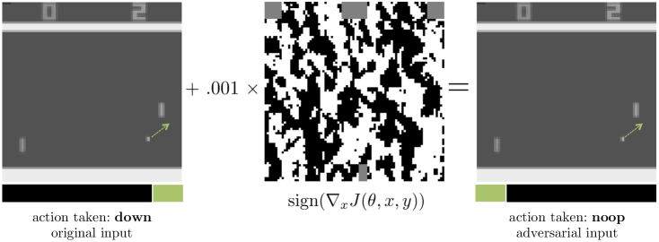
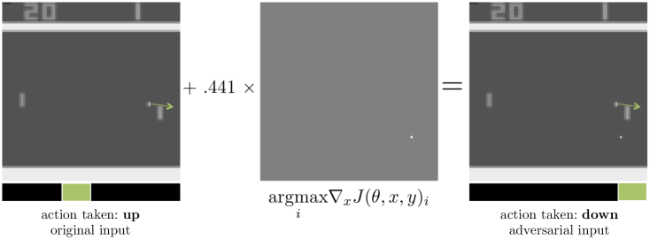
Our main contribution is to characterize how the effectiveness of adversarial examples is impacted by two factors: the deep RL algorithm used to learn the policy, and whether the adversary has access to the policy network itself (white-box vs. black-box). We first analyze three types of white-box attacks on four Atari games trained with three deep reinforcement learning algorithms (DQN [15], TRPO [19], and A3C [16]). We show that across the board, these trained policies are vulnerable to adversarial examples. However, policies trained with TRPO and A3C seem to be more resistant to adversarial attacks. Fig. 1 shows two examples of adversarial attacks on a Pong policy trained with DQN, each at a specific time step during test-time execution.
Second, we explore black-box attacks on these same policies, where we assume the adversary has access to the training environment (e.g., the simulator) but not the random initialization of the target policy, and additionally may not know what the learning algorithm is. In the context of computer vision, Szegedy et al. [22] observed the transferability property: an adversarial example designed to be misclassified by one model is often misclassified by other models trained to solve the same task. We observe that the cross-dataset transferability property also holds in reinforcement learning applications, in the sense that an adversarial example designed to interfere with the operation of one policy interferes with the operation of another policy, so long as both policies have been trained to solve the same task. Specifically, we observe that adversarial examples transfer between models trained using different trajectory rollouts and between models trained with different training algorithms.
2 Related Work
Adversarial machine learning [2], and more generally the security and privacy of machine learning [18], encompasses a line of work that seeks to understand the behavior of models and learning algorithms in the presence of adversaries. Such malicious individuals can target machine learning systems either during learning by tampering with the training data [6], or during inference by manipulating inputs on which the model is making predictions [5]. Among the perturbations crafted at test time, a class of adversarial inputs known as adversarial examples was introduced by [22]. This first demonstration of the vulnerability of — then state-of-the-art — architectures to perturbations indistinguishable to the human eye led to a series of follow-up work showing that perturbations could be produced with minimal computing resources [10] and/or with access to the model label predictions only (thus enabling black-box attacks) [17], and that these perturbations can also be applied to physical objects [11, 20].
Most work on adversarial examples so far has studied their effect on supervised learning algorithms. A recent technical report studied the scenario of an adversary interfering with the training of an agent, with the intent of preventing the agent from learning anything meaningful [3]. Our work is the first to study the ability of an adversary to interfere with the operation of an RL agent by presenting adversarial examples at test time.
3 Preliminaries
In this section, we describe technical background on adversarial example crafting and deep reinforcement learning, which are used throughout the paper.
3.1 Adversarial Example Crafting with the Fast Gradient Sign Method
Techniques for crafting adversarial examples generally focus on maximizing some measure of harm caused by an adversarial perturbation, constrained by some limit on the size of the perturbation intended to make it less noticeable to a human observer. A range of crafting techniques exist, allowing the attacker to choose an attack that makes the right tradeoff between computational cost and probability of success.
For exploratory research purposes, it is common to use a computationally cheap method of generating adversarial perturbations, even if this reduces the attack success rate somewhat. We therefore use the Fast Gradient Sign Method (FGSM) [10], an existing method for efficiently generating adversarial examples in the context of computer vision classification. The FGSM is fast because it makes a linear approximation of a deep model and solves the maximization problem analytically, in closed form. Despite this approximation, it is still able to reliably fool many classifiers for computer vision problems, because deep models often learn piece-wise linear functions with surprisingly large pieces.
FGSM focuses on adversarial perturbations where each pixel of the input image is changed by no more than . Given a linear function , the optimal adversarial perturbation that satisfies is
| (1) |
since this perturbation maximizes the change in output for the adversarial example , .
Given an image classification network with parameters and loss , where is an image and is a distribution over all possible class labels, linearizing the loss function around the input results in a perturbation of
| (2) |
3.2 Deep Reinforcement Learning
Reinforcement learning algorithms train a policy to optimize the expected cumulative reward received over time. For a given state space and action space , the policy may be a deterministic function mapping each state to an action: , or it may be a stochastic function mapping each state to a distribution over actions: , where is the probability simplex on . Here, the state space may consist of images or low-dimensional state representations. We choose to represent by a function parametrized by , for instance may be a weighting on features of the state [1]. In the case of deep reinforcement learning, are the weights of a neural network. Over the past few years, a large number of algorithms for deep RL have been proposed, including deep Q-networks (DQN) [15], trust region policy optimization (TRPO) [19], and asynchronous advantage actor-critic (A3C) [16]. We compare the effectiveness of adversarial examples on feed-forward policies trained with each of these three algorithms.
3.2.1 Deep Q-Networks
Instead of modeling the policy directly, a DQN [15] approximately computes, for each state, the Q-values for the available actions to take in that state. The Q-value for a state and action is the expected cumulative discounted reward obtained by taking action in state , and following the optimal policy thereafter. A DQN represents the Q-value function via a neural network trained to minimize the squared Bellman error, using a variant of Q-learning. As this is off-policy learning, it employs an -greedy exploration strategy. To reduce the variance of Q-learning updates, experience replay is used: samples are randomly drawn from a replay buffer (where all recent transitions are stored) so that they are not correlated due to time. The corresponding policy for a DQN is obtained by choosing the action with the maximum Q-value for each state, hence it is deterministic.
3.2.2 Trust Region Policy Optimization
TRPO [19] is an on-policy batch learning algorithm. At each training iteration, whole-trajectory rollouts of a stochastic policy are used to calculate the update to the policy parameters , while controlling the change in the policy as measured by the KL divergence between the old and new policies.
3.2.3 Asynchronous Advantage Actor-Critic
A3C [16] uses asynchronous gradient descent to speed up and stabilize learning of a stochastic policy. It is based on the actor-critic approach, where the actor is a neural network policy and the critic is an estimate of the value function . During learning, small batches of on-policy samples are used to update the policy. The correlation between samples is reduced due to asynchronous training, which stabilizes learning.
4 Adversarial Attacks
In our work, we use FGSM both as a white-box attack to compute adversarial perturbations for a trained neural network policy whose architecture and parameters are available to the adversary, and as a black-box attack by computing gradients for a separately trained policy to attack using adversarial example transferability [22, 10, 17].
4.1 Applying FGSM to Policies
FGSM requires calculating , the gradient of the cost function with respect to the input . In reinforcement learning settings, we assume the output is a weighting over possible actions (i.e., the policy is stochastic: ). When computing adversarial perturbations with FGSM for a trained policy , we assume the action with the maximum weight in is the optimal action to take: in other words, we assume the policy performs well at the task. Thus, is the cross-entropy loss between and the distribution that places all weight on the highest-weighted action in .111Functionally, this is equivalent to a technique introduced in the context of image classification, to generate adversarial examples without access to the true class label [12].
Of the three learning algorithms we consider, TRPO and A3C both train stochastic policies. However, DQN produces a deterministic policy, since it always selects the action that maximizes the computed Q-value. This is problematic because it results in a gradient of zero for almost all inputs . Thus, when calculating for policies trained with DQN, we define as a softmax of the computed Q-values (with a temperature of 1). Note that we only do this for creating adversarial examples; during test-time execution, policies trained with DQN are still deterministic.
4.2 Choosing a Norm Constraint
Let be the adversarial perturbation. In certain situations, it may be desirable to change all input features by no more than a tiny amount (i.e., constrain the -norm of ), or it may be better to change only a small number of input features (i.e., constrain the -norm of ). Thus we consider variations of FGSM that restrict the - and -norm of , as well as the original version of FGSM that restricts the -norm (Sec. 3.1).
Linearizing the cost function around the current input , the optimal perturbation for each type of norm constraint is:
| (3) |
where is the number of dimensions of input .
Note that the -norm and -norm constraints have adjusted to be the - and -norm of the vector , respectively, since that is the amount of perturbation under the -norm constraint. In addition, the optimal perturbation for the -norm constraint either maximizes or minimizes the feature value at dimensions of the input, ordered by decreasing . For this norm, the adversary’s budget — the total amount of perturbation the adversary is allowed to introduce in the input — is .
5 Experimental Evaluation
We evaluate our adversarial attacks on four Atari 2600 games in the Arcade Learning Environment [4]: Chopper Command, Pong, Seaquest, and Space Invaders. We choose these games to encompass a variety of interesting environments; for instance, Chopper Command and Space Invaders include multiple enemies.
5.1 Experimental Setup
We trained each game with three deep reinforcement learning algorithms: A3C [16], TRPO [19], and DQN [15].
For DQN, we use the same pre-processing and neural network architecture as in [15] (Appendix A). We also use this architecture for the stochastic policies trained by A3C and TRPO. Specifically, the input to the neural network policy is a concatenation of the last 4 images, converted from RGB to luminance (Y) and resized to . Luminance values are rescaled to be from 0 to 1. The output of the policy is a distribution over possible actions.
For each game and training algorithm, we train five policies starting from different random initializations. For our experiments, we focus on the top-performing trained policies, which we define as all policies that perform within of the maximum score for the last ten training iterations. We cap the number of policies at three for each game and training algorithm. Certain combinations (e.g., Seaquest with A3C) had only one policy meet these requirements.
In order to reduce the variance of our experimental results, the average return for each result reported is the average cumulative reward across ten rollouts of the target policy, without discounting rewards.
5.2 Vulnerability to White-Box Attacks
First, we are interested in how vulnerable neural network policies are to white-box adversarial-example attacks, and how this is affected by the type of adversarial perturbation and by how the policy is trained. If these attacks are effective, even small adversarial perturbations (i.e., small for FGSM) will be able to significantly lower the performance of the target trained network, as observed in [10] for image classifiers. We evaluate multiple settings of across all four games and three training algorithms, for the three types of norm-constraints for FGSM.
5.2.1 Observations
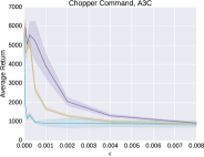
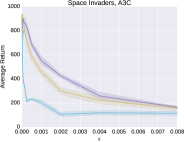
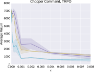
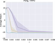
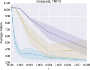
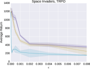
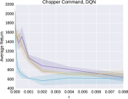
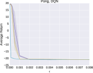
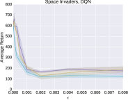
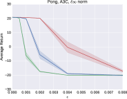
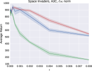
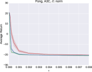
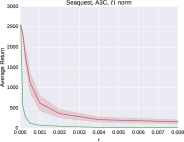
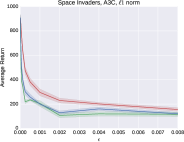
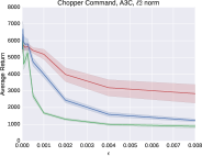
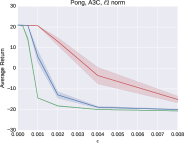
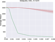
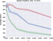
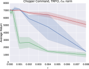
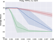
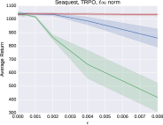
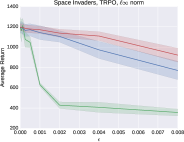
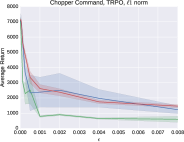
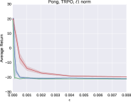
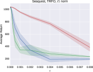
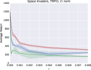
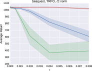
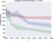
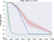
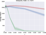
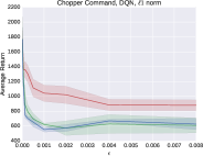
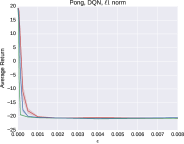
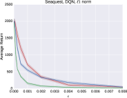
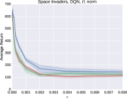
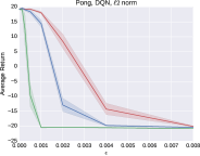
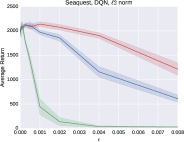
We find that regardless of which game the policy is trained for or how it is trained, it is indeed possible to significantly decrease the policy’s performance through introducing relatively small perturbations in the inputs (Fig. 2).
Notably, in many cases an -norm FGSM adversary with decreases the agent’s performance by or more; when converted to 8-bit image encodings, these adversarial inputs are indistinguishable from the original inputs.
In cases where it is not essential for changes to be imperceptible, using an -norm adversary may be a better choice: given the same , -norm adversaries are able to achieve the most significant decreases in agent performance. They are able to sharply decrease the agent’s performance just by changing a few pixels (by large amounts).
We see that policies trained with A3C, TRPO, and DQN are all susceptible to adversarial inputs. Interestingly, policies trained with DQN are more susceptible, especially to -norm FGSM perturbations on Pong, Seaquest, and Space Invaders.



5.3 Vulnerability to Black-Box Attacks
In practice, it is often the case that an adversary does not have complete access to the neural network of the target policy [17]. This threat model is frequently referred to as a black-box scenario. We investigate how vulnerable neural network policies are to black-box attacks of the following two variants:
-
1.
The adversary has access to the training environment and knowledge of the training algorithm and hyperparameters. It knows the neural network architecture of the target policy network, but not its random initialization. We will refer to this as transferability across policies.
-
2.
The adversary additionally has no knowledge of the training algorithm or hyperparameters. We will refer to this as transferability across algorithms.
5.3.1 Transferability Across Policies
To explore transferability of adversarial examples across policies, we generate adversarial perturbations for the target policy using one of the other top-performing policies trained with the same algorithm for the same task. We test all adversary-target combinations of top-performing policies trained with the same algorithm, for each combination of task, learning algorithm, and type of adversary.
5.3.2 Transferability Across Training Algorithms
To explore transferability of adversarial examples across training algorithms, we generate adversarial perturbations for the target policy using one of the top-performing policies trained with a different algorithm. Similarly, we test all adversary-target combinations of top-performing policies trained with different algorithms, for each combination of task and type of adversary.
5.3.3 Observations
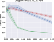
As one might expect, we find that the less the adversary knows about the target policy, the less effective the adversarial examples are (Fig. 3, 4, 5). Transferability across algorithms is less effective at decreasing agent performance than transferability across policies, which is less effective than when the adversary does not need to rely on transferability (i.e., the adversary has full access to the target policy network). However, for most games, transferability across algorithms is still able to significantly decrease the agent’s performance, especially for larger values of .
Notably for -norm adversaries, transferability across algorithms is nearly as effective as no transferability, for most game and algorithm combinations.








6 Discussion and Future Work
This direction of work has significant implications for both online and real-world deployment of neural network policies. Our experiments show it is fairly easy to confuse such policies with computationally-efficient adversarial examples, even in black-box scenarios. Based on [11], it is possible that these adversarial perturbations could be applied to objects in the real world, for example adding strategically-placed paint to the surface of a road to confuse an autonomous car’s lane-following policy.
Thus, an important direction of future work is developing defenses against adversarial attacks. This could involve adding adversarially-perturbed examples during training time (as in [10]), or it could involve detecting adversarial input at test time, to be able to deal with it appropriately.
References
- [1] P. Abbeel and A. Y. Ng. Apprenticeship learning via inverse reinforcement learning. In Proceedings of the Twenty-First International Conference on Machine Learning, 2004.
- [2] M. Barreno, B. Nelson, R. Sears, A. D. Joseph, and J. D. Tygar. Can machine learning be secure? In Proceedings of the 2006 ACM Symposium on Information, Computer and Communications Security, pages 16–25, 2006.
- [3] V. Behzadan and A. Munir. Vulnerability of deep reinforcement learning to policy induction attacks. arXiv preprint arXiv:1701.04143, 2017.
- [4] M. G. Bellemare, Y. Naddaf, J. Veness, and M. Bowling. The arcade learning environment: An evaluation platform for general agents. Journal of Artificial Intelligence Research, 47:253–279, 06 2013.
- [5] B. Biggio, I. Corona, D. Maiorca, B. Nelson, N. Šrndić, P. Laskov, G. Giacinto, and F. Roli. Evasion attacks against machine learning at test time. In Machine Learning and Knowledge Discovery in Databases, pages 387–402, 2013.
- [6] B. Biggio, B. Nelson, and L. Pavel. Poisoning attacks against support vector machines. In Proceedings of the Twenty-Ninth International Conference on Machine Learning, 2012.
- [7] M. Bojarski, D. D. Testa, D. Dworakowski, B. Firner, B. Flepp, P. Goyal, L. D. Jackel, M. Monfort, U. Muller, J. Zhang, X. Zhang, J. Zhao, and K. Zieba. End to end learning for self-driving cars. arXiv preprint arXiv:1604.07316, 2016.
- [8] G. Brockman, V. Cheung, L. Pettersson, J. Schneider, J. Schulman, J. Tang, and W. Zaremba. Openai gym, 2016.
- [9] Y. Duan, X. Chen, R. Houthooft, J. Schulman, and P. Abbeel. Benchmarking deep reinforcement learning for continuous control. In Proceedings of the Thirty-Third International Conference on Machine Learning, 2016.
- [10] I. J. Goodfellow, J. Shlens, and C. Szegedy. Explaining and harnessing adversarial examples. In Proceedings of the Third International Conference on Learning Representations, 2015.
- [11] A. Kurakin, I. Goodfellow, and S. Bengio. Adversarial examples in the physical world. arXiv preprint arXiv:1607.02533, 2016.
- [12] A. Kurakin, I. Goodfellow, and S. Bengio. Adversarial machine learning at scale. Proceedings of the Fifth International Conference on Learning Representations, 2017.
- [13] S. Levine, C. Finn, T. Darrell, and P. Abbeel. End-to-end training of deep visuomotor policies. Journal of Machine Learning Research, 17(39):1–40, 2016.
- [14] T. P. Lillicrap, J. J. Hunt, A. Pritzel, N. Heess, T. Erez, Y. Tassa, D. Silver, and D. Wierstra. Continuous control with deep reinforcement learning. In Proceedings of the Fourth International Conference on Learning Representations, 2016.
- [15] V. Mnih, K. Kavukcuoglu, D. Silver, A. Graves, I. Antonoglou, D. Wierstra, and M. Riedmiller. Playing atari with deep reinforcement learning. In NIPS Workshop on Deep Learning, 2013.
- [16] V. Mnih, A. Puigdomenech Badia, M. Mirza, A. Graves, T. P. Lillicrap, T. Harley, D. Silver, and K. Kavukcuoglu. Asynchronous methods for deep reinforcement learning. In Proceedings of the Thirty-Third International Conference on Machine Learning, 2016.
- [17] N. Papernot, P. McDaniel, I. Goodfellow, S. Jha, Z. B. Celik, and A. Swami. Practical black-box attacks against deep learning systems using adversarial examples. arXiv preprint arXiv:1602.02697, 2016.
- [18] N. Papernot, P. McDaniel, A. Sinha, and M. Wellman. Towards the science of security and privacy in machine learning. arXiv preprint arXiv:1611.03814, 2016.
- [19] J. Schulman, S. Levine, P. Moritz, M. I. Jordan, and P. Abbeel. Trust region policy optimization. In Proceedings of the Thirty-Second International Conference on Machine Learning, 2015.
- [20] M. Sharif, S. Bhagavatula, L. Bauer, and M. K. Reiter. Accessorize to a crime: Real and stealthy attacks on state-of-the-art face recognition. In Proceedings of the 2016 ACM SIGSAC Conference on Computer and Communications Security, pages 1528–1540, 2016.
- [21] D. Silver, A. Huang, C. J. Maddison, A. Guez, L. Sifre, G. van den Driessche, J. Schrittwieser, I. Antonoglou, V. Panneershelvam, M. Lanctot, S. Dieleman, D. Grewe, J. Nham, N. Kalchbrenner, I. Sutskever, T. Lillicrap, M. Leach, K. Kavukcuoglu, T. Graepel, and D. Hassabis. Mastering the game of go with deep neural networks and tree search. Nature, 529:484–503, 2016.
- [22] C. Szegedy, W. Zaremba, I. Sutskever, J. Bruna, D. Erhan, I. Goodfellow, and R. Fergus. Intriguing properties of neural networks. In Proceedings of the Second International Conference on Learning Representations, 2014.
Appendix A Experimental Setup
We set up our experiments within the rllab [9] framework. We use a parallelized version of the rllab implementation of TRPO, and integrate outside implementations of DQN222github.com/spragunr/deep_q_rl and A3C333github.com/muupan/async-rl. We use OpenAI Gym environments [8] as the interface to the Arcade Learning Environment [4].
The policies use the network architecture from [15]: a convolutional layer with 16 filters of size with a stride of 4, followed by a convolutional layer with 32 filters of size with a stride of 2. The last layer is a fully-connected layer with 256 hidden units. All hidden layers are followed by a rectified nonlinearity.
For all games, we set the frame skip to 4 as in [15]. The frame skip specifies the number of times the agent’s chosen action is repeated.
A.1 Training
We trained policies with TRPO and A3C on Amazon EC2 c4.8xlarge machines. For each policy, we ran TRPO for 2,000 iterations of 100,000 steps each, which took 1.5 to 2 days. We set the bound on the KL divergence to 0.01, as in [19].
For A3C, we used 18 actor-learner threads and a learning rate of 0.0004. As in [16], we use an entropy regularization weight of 0.01, use RMSProp for optimization with a decay factor of 0.99, update the policy and value networks every 5 time steps, and share all weights except the output layer between the policy and value networks. For each policy, we ran A3C for 200 iterations of 1,000,000 steps each, which took 1.5 to 2 days.
For DQN, we trained policies on Amazon EC2 p2.xlarge machines. We used 100,000 steps per epoch and trained for two days.