Modelling the UV to radio SEDs of nearby star-forming galaxies: new PARSEC SSP for GRASIL

Abstract

By means of the updated PARSEC database of evolutionary tracks of massive stars, we compute the integrated stellar light, the ionizing photon budget and the supernova rates of young simple stellar populations (SSPs), for different metallicities and IMF upper mass limits. Using CLOUDY we compute and include in the SSP spectra the nebular emission contribution. We also revisit the thermal and non-thermal radio emission contribution from young stars. Using GRASIL we can thus predict the panchromatic spectrum and the main recombination lines of any type of star-forming galaxy, including the effects of dust absorption and re-emission. We check the new models against the spectral energy distributions (SEDs) of selected well-observed nearby galaxies. From the best-fit models we obtain a consistent set of star formation rate (SFR) calibrations at wavelengths ranging from ultraviolet (UV) to radio. We also provide analytical calibrations that take into account the dependence on metallcity and IMF upper mass limit of the SSPs. We show that the latter limit can be well constrained by combining information from the observed far infrared, 24 $\micron$, 33 GHz and H$\alpha$ luminosities. Another interesting property derived from the fits is that, while in a normal galaxy the attenuation in the lines is significantly higher than that in the nearby continuum, in individual star bursting regions they are similar, supporting the notion that this effect is due to an age selective extinction. Since in these conditions the Balmer decrement method may not be accurate, we provide relations to estimate the attenuation from the observed 24 $\micron$ or 33 GHz fluxes. These relations can be useful for the analysis of young high redshift galaxies.

1 Introduction

Modelling the SEDs of galaxies has proven to be a very powerful tool in our current understanding of the different physical processes that come into play in the formation and evolution of galaxies. Various physical properties of galaxies like stellar, metal and dust content, star formation rate, dust obscuration, etc are estimated by fitting the theoretical SEDs to the observed ones. In the UV to infrared (IR) spectral regions of a SED, dust plays an important role. It absorbs (as well as scatters) the UV-near-infrared (NIR) light and re-radiates it in the IR. This IR emission (3 - 1000 $\micron$) may arise from (a) the emission from dust heated by young OB stars (neglecting heating from AGN), (b) the emission from the circumstellar envelopes of evolved stars and (c) the cirrus emission from dust distributed throughout in the ISM and heated by the general interstellar radiation field. Point (b) leads to wrong estimates of the physical properties related to star formation. The radio band which is not sensitive to dust attenuation is usually used to check and complement the interpretations arrived by using the optical/IR bands. Radio emission from normal star-forming galaxies is usually dominated by the non-thermal component (up to $\approx$ 90 per cent of the radio flux) which is believed to be due to the synchrotron emission from relativistic electrons accelerated into the shocked ISM by core-collapse supernovae (CCSN) explosions from massive young stars (above  $\approx 8~{}\rm{M}_{\sun}$) ending their lifes (Condon, 1992). Recent advances in hydrodynamical simulations of CCSN have indicated a range of stellar masses where the stars fail to explode but rather end up directly as a black hole. This raises concern about the widely accepted notion that all stars more massive than $\approx 8~{}\rm{M}_{\sun}$ end up as a CCSN.

Over the years, great progress has been made both in the development of tools and models use to extract the information encoded in the SEDs and in multi-wavelength surveys that sample the UV to radio SED of local and high redshift galaxies. Furthermore, new observing facilities with unprecedented resolution and sensivity (e.g. SKA, JWST, EVLT etc) will be put in place in the nearest feature. At the same time, semi-analytic models of galaxy formation, in the context of the current cosmological standard model, are appearing and providing realistic predictions of the physical properties of galaxies with which the results of the SED fitting can be compared.

Stellar population synthesis (SPS) still remains the basis of SED modelling. The most common method used in computing the SEDs of SSPs is that of isochrone synthesis (Chiosi, Bertelli & Bressan, 1988; Maeder & Meynet, 1988; Charlot & Bruzual, 1991) which uses the locus of stars in an isochrone to integrate the spectra of all stars along an isochrone to get the total flux. This involves computing first the stellar evolutionary tracks for different masses and metal contents and building the isochrones from the tracks. With the isochrones, the resulting stellar spectrum is computed using stellar atmosphere libraries. In recent years, significant efforts from different research groups have been put into providing homogeneous sets of evolutionary tracks and improving the stellar libraries. As a result of these improvements, SPS models can remarkably reproduce well the UV-NIR SEDs and high-resolution spectra in the optical wavelength band. However, despite these improvements, there are still challenges in the field, especially in the treatment of the phases of stellar evolution that are weakly understood. The most important being the short lived phases: massive stars, thermally pulsing asymptotic giant branch (TP-AGB) stars, blue stragglers and extreme horizontal branch stars. The TP-AGB stars have however increasingly received attention leading to a rapid progress in their modelling (Maraston, 2005; Marigo & Girardi, 2007; Marigo et al., 2017).

The stellar evolution code used in Padova to compute sets of stellar evolutionary tracks that are of wide useage in the astronomical community has recently been thoroughly revised and updated, going by the name, PARSEC(PAdova-TRieste Stellar Evolution Code). More details of this code can be found in Bressan et al. (2012, 2013); Chen et al. (2014) and will be briefly discussed later in the text. In this paper, our main aim is to use the PARSEC evolutionary tracks of massive stars to compute the quantities (the integrated light, ionizing photon budget and the supernova rates) of young SSPs, thereby updating the SSPs used by GRASIL in predicting the panchromatic spectrum of star-forming galaxies. We also revisit the thermal and non-thermal radio emissions. We finally check these new models with selected nearby well-observed galaxies. We perform an analysis of the resulting best-fit SEDs, with the aim of obtaining a new set of SFR calibrations and investigating the dependence of the dust attenuation properties on galaxy types.

The structure of the rest of paper is as follows: In Section 2, we use the new PARSEC code database of stellar evolutionary tracks of massive stars to compute the ionizing photon budget, the integrated light and the supernova rates predicted by young SSP models. Using the integrated spectra of the SPPs in CLOUDY, we computed the nebular emissions. In Section 3, we revise (a) the prescription used in computing the thermal radio emission. (b) the previous non-thermal radio emission model originally described in Bressan, Silva & Granato (2002, hereafter B02) while taking into account recent advances in CCSN explosion models. In Section 4, we check our new radio emission models and SSPs with GRASIL using selected well-observed nearby galaxies. Finally, we discuss the resulting best fit SEDs of all galaxies studied in this paper in Section 5. We draw our conclusions in Section 6.

Throughout this paper we adopt $\rm{12}+\rm{log}(\rm{O/H})=8.69$ (Asplund et al., 2009) as the solar oxygen abundance. Our models adopt a Kennicutt (1983) IMF (slope of -1.4 for $0.1-1~{}\rm{M}_{\sun}$ and -2.5 for $\geq 1~{}\rm{M}_{\sun}$). The cosmological parameters we adopt assume $H_{0}=70~{}\rm{km}\;s^{-1}\;\rm{Mpc}^{-1},\Omega_{\Lambda}=0.7,\Omega_{M}=0.3$

2 Simple Stellar Populations with PARSEC

PARSEC is the latest version of the Padova-Trieste stellar evolution code with thorough update of the major input physics including new and accurate homogenised opacity and equation of state tables fully consistent with any adopted chemical composition. More details may be found in Bressan et al. (2012, 2013); Chen et al. (2014). The evolutionary tracks span a wide range in metallicities, $0.0001\leq Z\leq 0.04$, and initial masses, from very low $(M~{}=~{}0.1~{}\rm{M}_{\sun})$ to very massive $(M~{}=~{}350~{}\rm{M}_{\sun})$ stars, starting from the pre-main sequence phase and ending at central carbon ignition. Tang et al. (2014) and Chen et al. (2015) computed new evolutionary tracks of massive stars and tables of theoretical bolometric corrections that allow for the conversion from theoretical HR to the observed colour-magnitude diagrams. A preliminary comparison of the new models with color-magnitude diagrams of star-forming regions in nearby low metallicity dwarf irregular galaxies was performed by Tang et al. (2014). The full set of new evolutionary tracks and the corresponding isochrones may be found in http://people.sissa.it/~sbressan/parsec.html and http://stev.oapd.inaf.it/cgi-bin/cmd, respectively.

2.1 Integrated SSP spectra

To build the integrated spectra of SSPs, we adopt the spectral library compilation by Chen et al. (2015) who homogenized various sets of existing stellar atmosphere libraries encompassing a wide range of parameters of both cool and hot stars (i.e. masses, evolutionary stages and metallicities). The atmosphere models adopted by Chen et al. (2015) are the ATLAS9 models (Kurucz, 1993; Castelli & Kurucz, 2004), suitable for intermediate and low mass stars, and the Phoenix models (Allard et al., 1997) for the coolest stars. For hot massive stars Chen et al. (2015) generated new wind models with the WM-BASIC code Pauldrach, Puls & Kudritzki (1986) and adopted new models of WR stars from the Potsdam group (see e.g. Sander et al., 2015). Since different sets of libraries have different metallicities, they were merged to obtain homogeneous sets of spectral libraries as described in Girardi et al. (2002) and Chen et al. (2014).

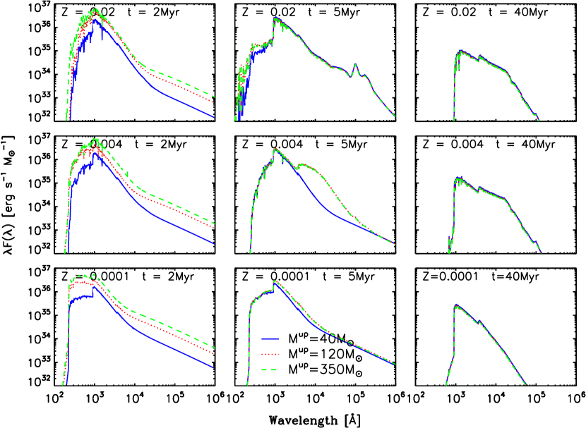
Figure 1: SSP Integrated spectra per solar mass at ages of $t~{}=~{}$2, 5 and 40 Myr, for metallicities Z = 0.02, 0.004 and 0.0001 and $\rm{M}_{up}$ of 40, 120 and 350 $\rm{M}_{\sun}$ indicated by the solid blue, dotted red and dashed green lines respectively. At 2 Myr, the spectra for the various upper mass limits at any of the three metallicities is quite distinguishable. At 5 Myr and Z = 0.02, it is distinguishable only at wavelengths below $912~{}\text{\AA}$, the maximum for the lyman ionizing photons. At this age, notice that the spectra for the $\rm{M}_{up}$ of 120 and 350$~{}\rm{M}_{\sun}$ below $912~{}\mbox{\AA}$ are superimposed, owing to the fact they must have evolved off the main sequence at this age. At 5 Myr and Z = 0.0001, the reverse is the case, the spectra is distinguishable only at wavelengths above $912~{}\text{\AA}$ because at this metallicity, stars lifetimes are a bit longer than at Z = 0.02. At 40 Myr, the spectra for all upper mass limits and metalicities are all superimposed and the Lyman ionizing photons are no longer produced.

The properties of SSP are obtained by integration along the corresponding isochrones assuming a two-slopes power law Kennicutt initial mass function. Results are presented for three different values of the upper mass limit, $\rm{M}_{up}$ of 40,120, 350 $\rm{M}_{\sun}$. As an example, Figure 1 shows the synthesized spectra of star clusters at ages of $t~{}=~{}$2, 5 and 40 Myr and for three values of the initial metallicity, Z = 0.02, 0.004 and 0.0001. The effect of assuming different $\rm{M}_{up}$ values, at fixed total initial mass, is more pronounced at an age of 2 Myr. At 5 Myr, when stars with masses of 120 $\rm{M}_{\sun}$ and 350 $\rm{M}_{\sun}$ already left the main sequence or already died out, the spectra of SSP with upper mass limits of 120 $\rm{M}_{\sun}$ and 350 $\rm{M}_{\sun}$ are superimposed, while those of 40 $\rm{M}_{\sun}$ remains distinct. At 40 Myr the spectra are almost independent of $\rm{M}_{up}$, though it is evident that the spectrum of the SSP with larger $\rm{M}_{up}$ has a lower luminosity, because of the higher mass budget stored in massive stars We already note from this figure that the effects of $\rm{M}_{up}$ on the number of ionizing photons disappears at ages larger than about 5 Myr, as discussed below.

2.2 Ionizing Photon Budget

The number of Lyman ionizing photons per sec ($\rm{Q(H)}$) and per unit mass emitted by young stellar populations is controlled by hot massive stars, i.e. O-B main sequence stars and Wolf Rayet stars. This number is thus critically dependent on the shape of the initial mass function in the domain of massive stars. In Figure 2, we show the time evolution of $\rm{Q(H)}$ for selected SSPs with different upper mass limit ($\rm{M}_{up}$) and metallicities. As already said, the adopted IMF is a two-slope power law Kennicutt (1983). The lower limit is $\rm{M}_{low}$ = 0.1 $\rm{M}_{\sun}$ and the upper limits are $\rm{M}_{up}$ = 40 $\rm{M}_{\sun}$, $\rm{M}_{up}$ = 120 $\rm{M}_{\sun}$ and $\rm{M}_{up}$ = 350 $\rm{M}_{\sun}$. The slope of the IMF is X = 1.4 between $\rm{M}_{low}$ and $\rm{M}$ = 1$\rm{M}_{\sun}$ and X = 2.5 between $\rm{M}$ = 1$\rm{M}_{\sun}$ and $\rm{M}_{up}$

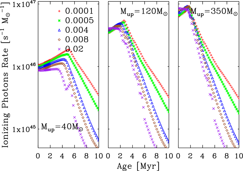
Figure 2: Variation of the instantenous number of ionizing photons per second per unit ionizing solar mass of the cluster with age (Myr). Different symbols correspond to different metallicities as illustrated in the plot

.

From this figure we may appreciate the role of age, metallicity and IMF on the ionizing photon rate $\rm{Q(H)}$. For a given Z and $\rm{M}_{up}$, $\rm{Q(H)}$ generally increases to a maximum value and then, once a threshold age is reached, it rapidly decreases to negligible values. At fixed $\rm{M}_{up}$, both the maximum value of $\rm{Q(H)}$ and the threshold age decrease, at increasing metallicity. In general this is also true at varying age, i.e. at given $\rm{M}_{up}$, $\rm{Q(H)}$ decreases at increasing metallicity. However there are some cases where this is not true, in particular for the SSP of solar metallicity. The effect of $\rm{M}_{up}$ is strong. A star cluster with $\rm{M}_{up}$ of 350 $\rm{M}_{\sun}$ produces about seven times more ionizing photons than a cluster with a $\rm{M}_{up}$ of 40 $\rm{M}_{\sun}$, at constant total mass. Moreover, the age to attain the maximum $\rm{Q(H)}$ becomes lesser at increasing upper mass limit, reflecting the larger relative weight of more massive stars in the ionizing photon budget.

2.3 Nebular Emission with PARSEC’s SSP

The integrated spectra of the SSPs are used to calculate the nebular emission from the surrounding H ii regions which is then added to the original spectrum to obtain the integrated spectra containing both the stellar continuum (with absorption lines and eventually wind emission features) and the nebular features (continuum and lines). For this purpose, star clusters are assumed to be the central ionizing sources of the H ii regions that are modelled using the photoionization code CLOUDY (Ferland, 1996). As a further input to the CLOUDY code, we specify that the H ii region is modelled as a thin shell of gas with constant density, $n_{H}=100~{}cm^{-3}$, placed at a distance $R_{H}$ = 15 pc from the central source. The evolution of the ionizing star clusters is followed from 0.1 Myr to 20 Myr, for five different values of the metallicity (Z = 0.0001, 0.0005, 0.004, 0.008, 0.008 and 0.02) and three values of $M_{up}$ of 40, 120 and 350 M_☉. We note that our goal is not that of providing a detailed dependence of a large ensemble of emission lines on the critical parameters of the H ii nebulae. Instead we aim at obtaining a reasonable estimate of the intensities of the main recombination lines and of free-free emission to increase the diagnostic capabilities of our population synthesis codes. Line emission and the corresponding nebular continuum are much less dependent on the characteristic properties of the H ii regions (e.g. ionization parameter, individual abundance of heavy elements etc.) than e.g. excitation lines, for which a more detailed set of initial parameters would be more appropriate (see e.g. Panuzzo et al., 2003; Wofford et al., 2016). The main output of this process is a library of emission line intensities, nebular continuum properties and electron temperatures (T_e) of the H ii regions. Then, emission lines and nebular continuum are used to suitably complement the integrated SED of SSPs from the far-UV to radio wavelengths.

3 RADIO CONTINUUM EMISSION

Radio emission associated with the presence of young massive stars comprises essentially two components, the thermal radio emission (also referred to as free-free emission) and the non-thermal radio emission (also referred to as non-thermal radio emission). The former emission comes from the nebular free electrons originating from the ionizing radiation of massive stars. The non-thermal emission is instead believed to be synchrotron radiation that originated from the interaction of relativistic electrons, produced in the ejecta of core-collapsed supernovae (CSSN), with the ambient magnetic field. The radio continuum is thus a tracer of the number of massive stars formed (and exploded) and hence an optimal indicator of the very recent (if not the current) star formation rate.

The fact that the radio emission is a good SFR tracer is supported by the remarkably tight correlation between FIR and non-thermal radio emission. At 1.49 GHz, this correlation is quantified by the q-parameter (Helou, Soifer & Rowan-Robinson, 1985):

$$q=\rm{log}\frac{F_{\rm{FIR}}/(3.75\times 10^{12}Hz)}{F_{\nu}(1.49\rm{GHz})/(W\;m^{-2}\;Hz^{-1})}\approx 2.35\pm 0.2$$ (1)

where $F_{\rm{FIR}}=1.26\times 10^{-14}(2.58S_{60\micron}+S_{100\micron})\rm{W}\rm{m}^{-2}$ (Young et al., 1989), $S_{60\micron}$ and $S_{100\micron}$ are IRAS flux densities in $\rm{Jy}$.

3.1 Thermal Radio Emission

At sufficiently high frequency such that free-free self-absorption is negligible, the relation between the specific luminosity of free-free emission $L_{\rm{ff}}(\nu)$ and the rate of ionizing photons $\rm{Q(H)}$ can be written as (Rubin, 1968; Condon, 1992)

$$L_{\rm{ff}}=\frac{\rm{Q(H)}}{C_{1}}\left(\frac{\rm{T}_{e}}{10^{4}\,\hbox{K}}\right)^{0.3}\,{\rm G_{dra}}(\nu,\hbox{T}_{e})\hskip 3.0pt$$ (2)

where $\rm{T}_{e}$ is the electron temperature, $C_{1}=\sqrt{3}/\pi\times 6.86\times 10^{26}$ and ${\rm G_{dra}}(\nu,\hbox{T}_{e})$ is the velocity averaged gaunt factor (Draine, 2011):

$$\hbox{G}_{\text{dra}}(\nu,\rm{T}_{e})=$$

$$\hbox{ln}\left\{\rm{exp}\left[5.960-{\frac{\sqrt{3}}{\pi}}\rm{ln}\left(Z_{i}{\frac{\nu}{\rm{GHz}}}\left({\frac{\rm{T_{e}}}{10^{4}\rm{K}}}\right)^{-1.5}\right)\right]+e\right\}$$ (3)

where $\rm{Z_{i}}$ is the charge of the ions in the H ii region. An approximate velocity averaged gaunt factor were obtained earlier by Oster (1961):

$$\hbox{G}_{\text{ost}}(\nu,\rm{T}_{e})=$$

$$\hbox{ln}\left[4.955\times 10^{-2}\left({\nu\over\hbox{GHz}}\right)^{-1}\right]+1.5\ \hbox{ln}\left({\hbox{T}_{e}\over\hbox{K}}\right)$$ (4)

Taking into account that $\hbox{G}_{\text{dra}}(\nu,\rm{T}_{e})\simeq\sqrt{3}/\pi\times\hbox{G}_{\text{ost}}(\nu,\rm{T}_{e})$ and adopting a common approximation used in literature, we obtain for the free-free emission (Condon, 1992)

$$\frac{L_{\rm ff}}{\hbox{erg}\,\hbox{s}^{-1}\,\hbox{Hz}^{-1}}={\frac{Q(H)}{6.3\times~{}10^{25}}}\left(\frac{\rm{T}_{e}}{10^{4}\,\hbox{K}}\right)^{0.45}\,\left({\nu\over\hbox{GHz}}\right)^{-0.1}$$ (5)

The latter equation is often used by assuming a fixed electronic temperature (10⁴ K) to provide useful analytical approximations at radio frequencies especially in the lack of nebular emission (see discussion in B02). Here we directly estimate the intensity of the thermal radio emission of our SSP from Cloudy with the procedure already described in Section 2.3. In Figure 3, we show the evolution of the 1.49 GHz and 33 GHz thermal radio emission for different metallicities, Z = 0.0001, 0.0005, 0.004, 0.008 and 0.02, and different $M_{up}$ of $40,120$ and $350~{}\rm{M}_{\sun}$. The effects of metallicity and $M_{up}$ on the thermal emission are easily noted. For example, at Z = 0.0001, the 1.4 GHz thermal emission for $M_{up}=120~{}\rm{M}_{\sun}$ is about 3 - 7 times larger than that for $M_{up}=40~{}\rm{M}_{\sun}$ In general by increasing the metallicity from Z = 0.0001 to Z = 0.02 the thermal radio emission decreases by a factor of about 3. Instead by increasing $M_{up}$ from 40 to 350 $\rm{M}_{\sun}$, thermal emission increases by about one order of magnitude. These important factors, that must be considered in the calibration of the relation between star formation rate and thermal radio emission, are discussed below.

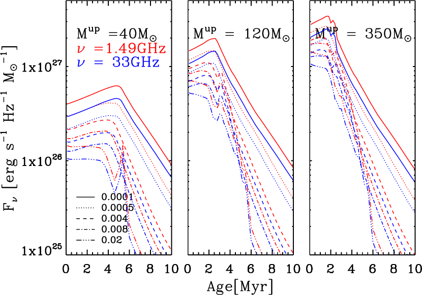
Figure 3: Variation of the 1.49GHz (red) and 33GHz (blue) thermal radio emission with age at different metallicities for different values of $M_{up}$. The five different line styles correspond to the five different values of metallicity.

3.1.1 Metallicity effects

Equations 2, 3 and 5 contain an explicit dependence on the electron temperature, that is generally neglected in analytical approximations which assume a constant value of $\rm{T_{e}}$ = 10⁴ K. Since $\rm{T_{e}}$ is known to depend on the metallicity of the H ii regions, with a variation of more than a factor of two in the range of the observed values, we provide in Appendix A some useful analytical relations. We first list in Table 2 the values of the electronic temperature derived using CLOUDY for our SSP models at various metallicities and upper mass limits. In Figure 17 of Appendix A, we show the relations between oxygen abundance and the electronic temperature. In this figure, crosses, ’X’s and asterisks indicate $M_{up}=40$, $120$ and $350~{}\rm{M}_{\sun}$ respectively. The average of the empirical fits derived by López-Sánchez et al. (2012) for high-ionization O iii and for low-ionization O iii zones is shown as the dashed black lines. We provide a multiple regression fitting relation (Equation 34) between $\rm{T_{e}}$, $\rm{M_{up}}$ and Z that could be easily included in analytical approximations.

3.1.2 $\rm{SFR}-\rm{Q(H)}$ calibration

In a young stellar system the ionizing photon budget is dominated by massive stars and thus there must be a tight relation between the current star formation rate and the rate of ionizing photons, that ultimately produce the thermal radio emission Condon & Yin (1990). In this section, we provide a calibration of the $\rm{SFR}-\rm{Q(H)}$ relation. For this purpose we consider the integrated spectrum of a galaxy up to a time $t$:

$$f_{\nu}^{gal}(t,Z)=\int_{0}^{t}f_{\nu}^{SSP}(t-t^{\prime},Z)SFR(t^{\prime})dt^{\prime}$$ (6)

where SFR(t’) is the star formation rate at time $t^{\prime}$ and $f_{\nu}^{SSP}(t-t^{\prime},Z)$ is the stellar spectrum of a SSP of age $t_{ssp}~{}=~{}t-t^{\prime}$ and given metallicity $Z$

$$f_{\nu}^{SSP}(t_{ssp},Z)=\int_{M_{low}}^{M_{up}}\phi(m)f_{\nu}(m,t_{ssp},Z)dm$$ (7)

In the latter equation, $f_{\nu}(m,t_{ssp},Z)$ is the spectrum of an individual star in a SSP which depends on the fundamental parameters, its mass $m$, age $t_{ssp}$, metal abundance $Z$ and the IMF, $\phi(m)$. Using the SSPs already described, a constant SFR of 10$~{}\rm{M_{\sun}}\;\rm{yr^{-1}}$ and adopting the Kennicutt (1983) IMF, we obtain the integrated number of ionizing photons $IQ(H)$, shown in figure 4. Since $IQ(H)$ is dominated by the most massive stars, the number of ionizing photons emitted by a galaxy with constant SFR will initially grow and soon saturate to a constant maximum value, when there is a balance between the newly formed ionizing massive stars and the ones that die. Looking at Figure 2 we see that, almost independently from the metallicity, the characteristic time of the saturation is set by the rapid drop of $IQ(H)$ above about 6 Myr. The effect of $\rm{M}_{up}$ on $IQ(H)$ is a direct consequence of the variation of the $Q(H)$ of SSPs shown in Figure 2. The variation of $\rm{IQ(H)}$ with metallicity decreases with increasing upper mass limit.

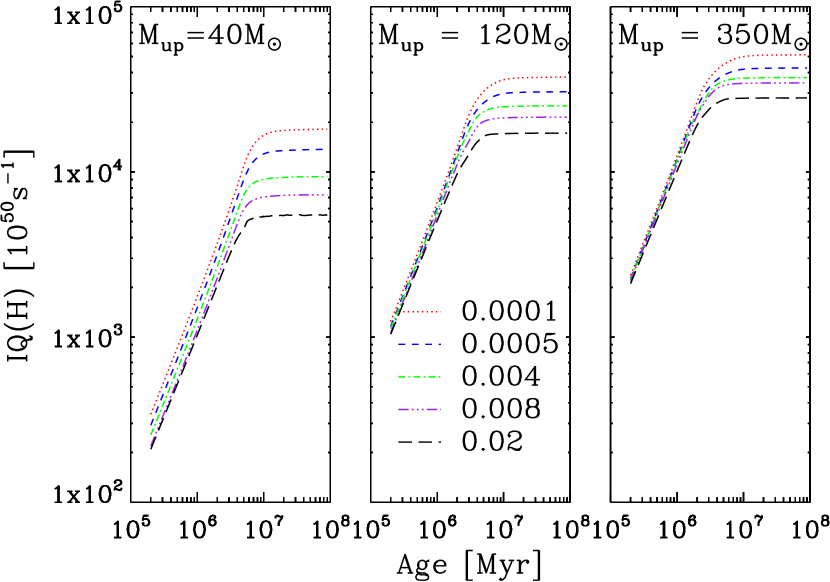
Figure 4: Evolution of the integrated number of ionizing photons per second per unit solar mass initially formed as a function of the age in yr. Different line colors represents different metallciities. The variation of Q(H) with metallicity decreasis at increasing IMF upper mass limit.

After denoting by $C_{2}$ the calibration coefficient between SFR and Q(H) in the equation below

$$\left({\frac{\rm{SFR}}{\rm{M}_{\sun}\;\rm{yr}^{-1}}}\right)=C_{2}\times\left(\frac{IQ(H)}{\rm{s^{-1}}}\right)$$ (8)

we collect in Table 2 the values of $C_{2}$ obtained with our constant SFR models, for different SSPs parameters. To illustrate the significant variations of $C_{2}$ with metallicity at a given $M_{up}$, we show in Figure 18 the plot of $C_{2}$ against metallicity for $M_{up}$ = 40, 120 and 350 $M_{\sun}$ Using the values of $C_{2}$ given in Table 2 for different $\rm{M}_{up}$ and $Z$ , we provide a multiple regression fitting relation between $C_{2}$ , $\rm{M}_{up}$ and metallicity ($Z$), Equation 35. As an example, using this fitting relation, for $M_{up}=120~{}\rm{M}_{\sun}$ and Z = 0.02 Equation 8 is:

$$\left({\frac{\rm{SFR}}{\rm{M}_{\sun}\;\rm{yr}^{-1}}}\right)=\left({\frac{IQ(H)}{s^{-1}}}\right)$$ (9)

We may compare equation 9 with the one obtained by Murphy et al. (2012) using the Starburst99 stellar population model with a Kroupa (2001) IMF, a metallicity of Z = 0.02 and a constant star formation over 100 Myr.

$$\left({\frac{\rm{SFR}}{\rm{M}_{\sun}\;\rm{yr}^{-1}}}\right)=\left({\frac{IQ(H)}{s^{-1}}}\right)$$ (10)

We see that the Murphy et al. (2012) calibration constant is fairly in agreement with ours.

3.1.3 SFR - $L_{ff}$ Calibration

By combining equation 8 and equation 2, we derive the relation between the SFR and thermal radio emission:

$$\frac{\rm{SFR}}{\rm{M_{\sun}yr^{-1}}}=\frac{L_{\rm{ff}}}{C_{3}}\left({\frac{\rm{T}_{e}}{10^{4}\hbox{K}}}\right)^{-0.3}\,\left(\frac{1}{G_{dra}}\right)$$ (11)

where $C_{3}=1/(C_{1}\times C_{2})$. The values of the coefficient $C_{3}$ for different SSP parameters are provided in Table 2 and the variation of $C_{3}$ with metallicity and $M_{up}$ is shown in Figure 19. Using these values of $C_{3}$ given in Table 2 for different $\rm{M}_{up}$ and $Z$, we also, as we did for the case $C_{2}$, provide a multiple regression fitting relation between $C_{3}$, $M_{up}$ and metallicity ($Z$), Equation 36. As an example, using this fitting relation for $M_{up}=120~{}\rm{M}_{\sun}$ and Z = 0.02 and assuming the already quoted approximation for the Gaunt factor, Equation 11 becomes

$$\frac{\rm{SFR}}{\rm{M_{\sun}\;yr^{-1}}}=\left(\frac{L_{\rm{ff}}}{2.77\times 10^{27}}\right)\left({\frac{\rm{T}_{e}}{10^{4}\hbox{K}}}\right)^{-0.45}\,\left(\frac{\nu}{\rm{GHz}}\right)^{0.1}$$ (12)

A similar equation is provided by Murphy et al. (2012):

$$\frac{\rm{SFR}}{\rm{M_{\sun}\;yr^{-1}}}=\left(\frac{L_{\rm{ff}}}{2.17\times 10^{27}}\right)\left(\frac{T_{e}}{10^{4}\rm{K}}\right)^{-0.45}\left(\frac{\nu}{\rm{GHz}}\right)^{0.1}$$ (13)

3.1.4 SFR versus H$\alpha$ and H$\beta$ calibrations

Using well-known relations between $IQ(H)$ and the intensity of recombination lines (Osterbrock, 1989), we may also obtain the corresponding calibrations for the SFR. For H$\alpha$ and H$\beta$ we have

$$\left(\frac{\rm{IQ(H)}}{\rm{s}^{-1}}\right)=7.31\times 10^{11}\left(\frac{L(H\alpha)}{\rm{erg}\;\rm{s}^{-1}}\right)$$ (14)

$$\left(\frac{\rm{IQ(H)}}{\rm{s}^{-1}}\right)=0.21\times 10^{13}\left(\frac{L(H\beta)}{\rm{erg}\;\rm{s}^{-1}}\right)$$ (15)

Using the above relations in equation 8, we write in Appendix A analytical equations for the SFR-H$\alpha$ (equation 39) and SFR-H$\beta$(equation 40) calibrations, as a function of Z and M_up. For the case with $M_{up}~{}=~{}120~{}\rm{M}_{\sun}$ and Z = 0.02 we obtain with these analytical equations

$$\left({\frac{\rm{SFR}}{\rm{M}_{\sun}\;\rm{yr}^{-1}}}\right)=4.79\times 10^{-42}\left({\frac{L(H\alpha)}{\rm{erg}\;\rm{s}^{-1}}}\right)$$ (16)

$$\left({\frac{\rm{SFR}}{\rm{M}_{\sun}\;\rm{yr}^{-1}}}\right)=0.14\times 10^{-40}\left({\frac{L(H\beta)}{\rm{erg}\;\rm{s}^{-1}}}\right)$$ (17)

Our calibration coefficient in equation  16 is in good agreement with the value of $4.55\times{10^{-42}}$ obtained by Bicker & Fritze-v. Alvensleben (2005) using GALEV synthesis code.

3.2 Non-Thermal Radio Emission

We know quite little about the source of non-thermal (NT) radio emission in star-forming galaxies. The mechanism is believed to be synchrotron emission from relativistic electrons that are accelerated by ISM shocks in the outskirts of CCSN explosions (Condon, 1992). B02 derived the following relation between NT radio emission $L^{NT}$ and the CCSN rate

$$\frac{L_{NT}/\frac{\nu_{CCSN}}{yr^{-1}}}{10^{30}~{}\rm{erg}\;\rm{s}^{-1}\;\rm{Hz}^{-1}} = E^{SNR}_{1.49}(\frac{\nu}{1.49})^{-0.5}+E^{NT}_{1.49}(\frac{\nu}{1.49})^{-\alpha}$$

(18)

In the above equation $\nu_{CCSN}$ is the CCSN rate, $E^{SNR}_{1.49}$ is the average non thermal radio luminosity due to a young Supernova Remnant (SNR) and $E^{NT}_{1.49}$ is the average injected energy in relativistic electrons per CCSN event. Moreover, B02 estimated that, at 1.49 GHz,

$$E^{SNR}\approx 0.06E^{NT}.$$ (19)

$E^{NT}_{1.49}$ can be estimated from observations. For our Galaxy B02 adopt $L^{NT}=6.1\times 10^{21}\;\rm{W}\;\rm{Hz}^{-1}$ (Berkhuijsen, 1984) at 0.4$\rm{GHz}$ and $\nu_{CCSN}=0.015$. They obtain for a radio slope $\alpha(\frac{-d\;\rm{log}S_{\nu}}{-d\;\rm{log}\nu})=0.8$, a value of $E^{NT}_{1.49}$ = 1.44. We note that the final fate of massive stars is a critical assumption for estimating their contribution to thermal radio emission. The formation of NSs and BHs depends on the amount of mass lost by the massive star through stellar winds and on the hydrodynamics of the explosion. One of the the most troublesome facts is that the variations shown by these pre-supernova stars in their structural properties, like for e.g. the Fe-core and O-core masses, are non-monotonic and pronounced even within small differences in the ZAMS masses (Sukhbold & Woosley, 2014). Some recent works in the attempt to characterize the parameters of successful and failed supernovae have yielded some structural parameters that can be utilized in predicting the fate of SNe (eg. Ertl et al., 2015; Ugliano et al., 2012; Janka, 2012; O’Connor & Ott, 2011). Using these parameters, Spera, Mapelli & Bressan (2015) and Slemer et al. 2017 (to be submitted) were able to characterize the final fate of PARSEC massive stars for the different criteria adopted for successful CCSN explosion. Following Spera, Mapelli & Bressan (2015) and Slemer et al. 2017 we assume that stars with initial mass above about $M=30~{}\rm{M}_{\sun}$ do not contribute to non thermal radio emission, contrary to B02 where all stars of masses above $M=8~{}\rm{M}_{\sun}$ were thought to explode as CCSN. The region between about $24-30~{}\rm{M}_{\sun}$ is critical because the explosion criterion by O’Connor & Ott (2011) produces a much higher number of NSs than that produced by Ertl et al. (2015) criterion. Finally we stress that we assume that progenitors undergoing pair-instability SNe either collapse to a BH or are completely incinerated by a thermonuclear explosion without producing relativistic electrons, similarly to what is assumed for SNIa. This assumption on the CCSN distribution with initial mass modifies the expected non thermal luminosity of star-forming galaxies and requires a re-calibration of the GRASIL model. After accounting for the failed and successful SNe in the evaluation of non thermal emission from Equation 18, we show in Figure 5 the variation of the 1.49 GHz non-thermal radio emissions with age, for different upper mass limits and metallicities. We note that non-thermal radio emission is not sensitive to the upper mass limit of the IMF, as long as it is larger than the assumed threshold for failed SN, M = 30$~{}\rm{M}_{\sun}$. In this case non thermal emission begins at an age of $\sim$7 Myr and not earlier ($\sim$3 Myr) as is the case in B02. By coincidence, this critical time corresponds to about the epoch at which thermal emission abruptly fades down, as depicted in Figure 5. Non thermal emission remains effective up to about 35 - 38 Myr, depending on the metallicity. In subsequent sections we will show how thermal and non-thermal radio emission are checked and eventually re-calibrated using the GRASIL code.

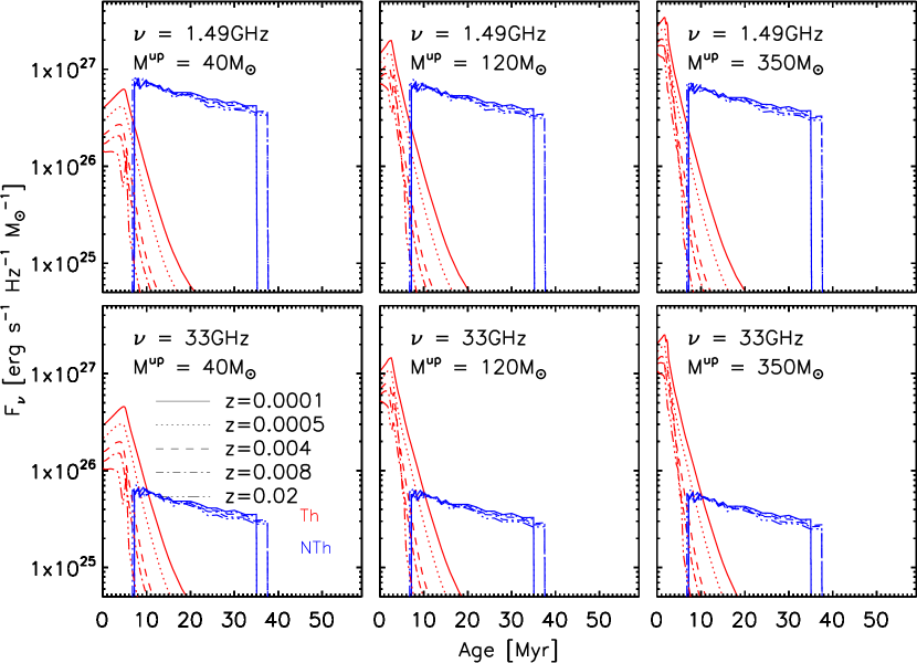
Figure 5: Variation of the 1.49 GHz and 33 GHz non-thermal (free-free) emission with age at different metallicities and different IMF upper mass limits. The red lines indicate thermal radio emission and the blue lines non-thermal radio emission. The plot for the thermal radio emission has already been shown in Figure 3 but added here for comparison with the non-thermal radio emission. As easily noticed in the figure, the non-thermal emission is almost unchanged for each of the different IMF upper mass limits, owing to the fact that masses above 30 $\rm{M}_{\sun}$ collapse directly to BH and do not explode to produce non-thermal emission. For this same reason, the non thermal emission for all plots starts at about an age of 7 Myr. For comparison purposes, the plot of the thermal radio emission is included to show it’s pronounced variation with upper mass limits. At 1.4 GHz (upper panel), the non-thermal radio emission dominates that at 33 GHz (lower panel) whereas at 33 GHz, the thermal emission dominates.

4 Calibration of the new SSP suite with GRASIL

In the previous sections, we described a new suite of SSPs that will supersede the ones used in the current version of GRASIL. The new suite differs in many aspects from the previous one as we briefly list in the followings. (1) The SSP are based on the most recent PARSEC stellar evolutionary tracks with an updated physics, in particular new mass-loss recipes and finer and wider coverage in initial mass and metallicity; (2) they include the most recent advances in our understanding of the CCSN explosion mechanism and account for the so called "failed SN"; (3) a more accurate gaunt factor and metallicity-dependent electron temperature were incorporated in the relation between the integrated ionization photon luminosity and thermal radio luminosity (4) in the current suite, we may adopt several values of the IMF upper mass limit Because of all these differences, we need to check and recalibrate some parameters of the SED produced by GRASIL, in particular to check whether we are able to reproduce the canonical value of $q_{1.4GHz}=2.35$, observed in a prototype normal star-forming galaxiy, see Eq. 1. For this purpose, in the next section we will use GRASIL with the new SSPs to reproduce the SEDs of a some selected well studied galaxies.

4.1 SED Modelling with GRASIL

GRASIL is a spectro-phometric code able to predict the SED of galaxies from the FUV to the radio, including state-of-the-art treatment of dust reprocessing (Silva et al., 1998, 2011; Granato et al., 2000), production of radio photons by thermal and non-thermal processes (BO2) and an updated treatment of PAH emission (Vega et al. (2005)). The reader is referred to these original papers for a fully detailed description of the code. It is also worth noting that nebular emission was already included in GRASIL by Panuzzo et al. (2003) but with a completely different procedure which also accounted for different electron densities. In this respect our procedure is more simple because nebular emission is added directly to the SSPs, but it allows a more versatile use of GRASIL.

For sake of convenience, we briefly summarise here the main features of GRASIL. The first step is to compute a chemical evolution model that provides the star formation history (SFH) and the metallicity and mass of the gas. Other quantities are computed by the code CHE$-$EVO, such as mass in stars, SN rates, detailed elemental abundances, but they are not used for the spectro-photometric synthesis. GRASIL’s main task is to compute the SED resulting from the interaction between the stellar radiation from CHE$-$EVO and dust, using a relatively flexible and realistic geometry where stars and dust are distributed in a spheroidal and/or a disk profiles. A spherical symmetric distribution with a King profile is adopted in the case of spheroidal systems while, for disk-like systems, a double exponential of the distance from the polar axis and from the equatorial plane is adopted. The dusty environments are made up of dust (i) in interstellar HI clouds heated by the general interstellar radiation of the galaxy (refered to as the cirrus component), (ii) associated with star-forming molecular clouds (MC) and (iii) in the circumstellar shells of Asymptotic Giant Branch (AGB) stars. GRASIL performs the radiative transfer of starlight through these environments. We remind the reader that the reprocessing of starlight by dust in envelopes of AGB stars is already taken into account in our SSPs. For the intrinsic dust properties, GRASIL adopts grains (graphite and silicate) in thermal equilibrium and a mixture of smaller grains and PAHs fluctuating in temperature. The dust parameters are tuned in order to match with the observed emissivity and extinction properties of the local ISM (Vega et al., 2005).

4.1.1 M100: a close to solar metallicity galaxy

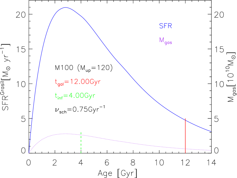
Figure 7: Star formation history of M100 adopted in our CHE-EVO model. The model parametrs are labelled: galaxy’s age (solid red line) , infall time (dashed green line) and schmidt-law efficiency. These parameters were adopted by Silva et al. (1998) based on constraints to reproduce the observed final mass of M100. The SFH is indicated by the solid blue lines while the gas mass history by the dotted purple line.

The galaxy M100 was selected from the Spitzer Nearby Galaxies Survey (SINGS) (Kennicutt et al., 2003), a collection of 75 nearby galaxies with a rich data coverage from the far-UV to the radio, because it is one of the best sampled objects, including the intensities of main emission lines. This will provide the opportunity to check, for the first time in GRASIL, the consistency of the SED continuum and emission lines fitting. To obtain the chemical evolution model we adopt the parameters of the chemical evolution code CHE-EVO given by Silva et al. (1998) who was able to well-reproduce M100. They are infall time scale $t_{inf}~{}=~{}4.0$ Gyr, efficiency of the Schmidt-law star formation law $\nu_{sch}~{}=~{}0.75$ and the total infall mass $m_{inf}$ = $2\times 10^{11}~{}M_{\sun}$. Figure 7 shows the SFH resulting from the adopted chemical evolution parameters. The SFH is indicated by the solid blue line and the gas mass history by the dotted purple line. To perform the SED fit, we consider several time steps along the chemical evolution of the galaxy for which we built a library of SED models with different GRASIL parameters. We note that since the observed SED refers to the whole galaxy, the derived parameters correspond to a luminosity average of the physical properties, as commonly obtained by this kind of fitting process. As a particular check, we also investigate the effect of changing the upper mass limit of the IMF, $\rm{M}_{up}~{}=~{}40$,120 and $350~{}M_{\sun}$, on some physical quantities derived from our best-fit SED, in particular the SFR. The main GRASIL parameters varied are the molecular gas fraction $f_{mol}$ , the escape time $t_{esc}$ and the optical depth of molecular clouds (MC) at 1$\micron$ $\tau_{1}$. The best fits were obtained by minimizing the merit function $\chi^{2}$ which is given by

$$\chi^{2}=\frac{1}{N}\sum^{N}_{i=1}\left(\frac{F_{mod}(i)-F_{obs}(i)}{Err(i)}\right)^{2}$$ (20)

where $F_{mod}(i)$, $F_{obs}(i)$ and $Err(i)$ are the model flux values, the observed fluxes and observational errors respectively. $N$ is the number of photometric bands used to obtain the best fit. Our GRASIL best-fit SEDs of M100 for $M_{up}=40~{}\rm{M}_{\sun}$ and $M_{up}=120~{}\rm{M}_{\sun}$, are shown in the left and right panels of Figure 6 respectively, while the corresponding best fit parameters are summarized in Table  1. We do not show the case with $M_{up}=350~{}\rm{M}_{\sun}$, because its thermal-radio emission was significantly exceeding the observed one. This discrepancy could not be cured by varying any other parameter in the fit. This result is, by itself, quite interesting and shows that for a normal star-forming galaxy it is difficult to have an average IMF extending up to such high initial masses. The different dust components in diffuse medium (cirrus) and molecular clouds are shown and indicated by the blue and red dashed lines, respectively. The thermal and non-thermal radio emission components are indicated by the cyan and purple dashed dotted lines, respectively. The thermal component can be seen to be negligible for the case of $M_{up}=40~{}\rm{M}_{\sun}$. We include, for the first time in GRASIL, selected emission lines in the SED. The labels in the plots refer to some important quantities derived from our best fit: the bolometric luminosity from UV to radio (BOL), the total IR luminosity from 3 - 1000$\micron$ (FIR), the predicted extinction uncorrected $H_{\alpha}$ luminosity (Ha^gra), the observed $H_{\alpha}$ luminosity (Ha^dat), $H_{\alpha}$ attenuation (A(H$\alpha$)), attenuation in the V($0.55\micron$) band (A(V)), the SFR averaged over the last 100 Myr ($<\rm{SFR}>$), the q-parameter as defined by equation 1 (q(1.4GHz)), the coefficients of the SFR(H_α) and SFR(IR) calibrations ($<\rm{SFR}/Ha>$ and $<\rm{SFR}/FIR>$ respectively). A summary of other important quantities derived from our best fit is provided in Tables 3 and  4. For both values of the adopted $M_{up}$, the best fits match very well the overall observed UV-radio SEDs. However, for $M_{up}$ = 120$~{}\rm{M}_{\sun}$, the model over-predicts by factor of $\sim$3 the observed (i.e. non corrected by extinction, hereafter ’transmitted’) H${\alpha}$ luminosity, $1.23\times 10^{41}\text{ergs}\;\text{s}^{-1}$ (taken from Kennicutt et al. (2009)). This upper mass limit also produces a higher UV emission and a slight excess of thermal emission. On the other hand, the observed H${\alpha}$ luminosity is well reproduced in the case of $M_{up}=40~{}\rm{M}_{\sun}$. The over-predicted H${\alpha}$ luminosity resulting from adopting $M_{up}$ = 120 $\rm{M}_{\sun}$ could be lowered by increasing the escape time of young stars in their parent clouds, leading to a larger absorption in the MCs. This will also lower the predicted far-UV emission which, in the current best fit, is slightly larger than the observed value. However, a larger absorption from MCs will increase the predicted $24~{}\micron$ flux above the observed one. Note that at $24~{}\micron$ the cirrus component has a pronounced minimum and its contribution to the overall MIR emission is only a small fraction of the total. Thus, the $24~{}\micron$ flux, being dominated by the MC emission, is indeed a strong diagnostic for the amount of light reprocessed by the MC component. From our best fit, we obtain a CCSN rate to NT radio luminosity ratio (Equation 18) that is about a factor of 1.35 larger than the value obtained by B02 using the previous radio model. That is,

$$E^{NT}_{1.49}(\rm{Thiswork})=1.944=E^{NT}_{1.49}(\rm{B02})\times 1.35$$ (21)

We anticipate here that this value is confirmed by all subsequent SED fits. We also note that this value is almost independent from the adoption of $M_{up}$ for the reasons already discussed previously. The predicted average SFR resulting from the panchromatic fit is only slightly affected by the adoption of a different value of $M_{up}$. By increasing $M_{up}$ from 40 to 120 $~{}\rm{M}_{\sun}$ the average SFR decreases by about 16 per cent.

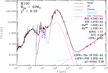
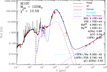
Figure 6: M100 GRASIL best-fit SED for $M_{up}$ = 40 $\rm{M}_{\sun}$ (right panel) and $M_{up}=120~{}\rm{M}_{\sun}$(left panel). The different dust components, diffuse medium and molecular clouds are represented by the dashed blue and red lines respectively. The thermal and non thermal radio components are represented by the cyan and purple dashed dotted lines. The thermal component can be seen to be negligible for the case of $M_{up}=40~{}\rm{M}_{\sun}$. For the different $M_{up}$, note the differences in the predicted quantities labelled in the plots (see text for more details), in particular the H_α luminosities, attenuations (A(H_α)) and SFR(H_α) calibration coefficient. We estimated $E^{NT}_{1.49}=1.944$, a factor of 1.35 larger than that obtained in B02. Our average value of q = 2.4 which is in line with the observed value of 2.35 (Equation 1) is an indication of our good calibration.

4.1.2 NGC 6946: individual star-bursting regions

In the previous section we were able to reproduce fairly well the observed SEDs of the prototype galaxy M100, in particular, we used the best fit model to calibrate the constant $E_{NT}$ of the non-thermal radio emission model. In this section we wish to check the thermal component of our radio emission model. For this purpose, we compare our synthetic SEDs with those of selected extranuclear regions of NGC 6946, a well studied starburst galaxy at a distance of 6.8 Mpc. This galaxy is dominated by very young starburst regions and shows relatively large thermal over non-thermal ratios (eg Israel & Kennicutt, 1980; Heckman et al., 1983), and thus is particularly well suited for a test of the free-free emission originating from star formation. Murphy et al. (2010) observed these regions at 1.4, 1.5, 1.7, 4.9, 8.5 and 33 GHz and complemented their full SEDs with existing data from the UV to the submm range. For eight observed regions Murphy et al. (2010) estimated an average 33 GHz thermal component of $\approx$ 85 per cent of the total, while for one region (named extra-nuclear region 4), this percentage was found to be significantly lower, $\approx$ 42  per cent, likely for the presence of a so-called anomalous dust emission component which suppresses the thermal component. Particulary interesting for our purpose is that Murphy et al. (2010) also provide the intensity of the H$\alpha$ emission for each region, that can be directly compared to the predictions of our model.

To model the SEDs of the extra-nuclear star-forming regions of NGC 6946 we adopt a spherical symmetric distribution with a King profile for the stars and dust. Most important, we use the data not corrected for the local background emission of the galaxy, though (Murphy et al., 2011) provide also data corrected for this emission. We thus adopt, for each region, a chemical evolution model composed by a star-burst superimposed to a quiescent star formating component. Our choice is dictated by the fact that the subtraction by (Murphy et al., 2011) may bias our results and we prefer to eventually split the contribution of the starburst and the old disk components directly from our fits.

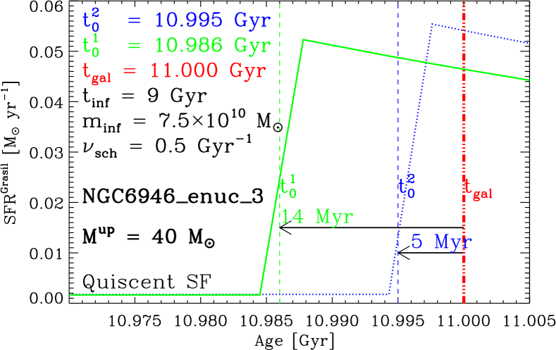
Figure 8: SFH of one of the 8 extranuclear regions, NGC 6946_enuc_3 for $M_{up}=40~{}M_{\sun}$ case. A starburst age of $t_{sb}^{1}$ = 14 Myr (green solid line) produced the best fit but we added $t_{sb}^{2}$= 5 Myr (blue dotted line) case only to illustrate that we do not expect any contribution to the non-thermal emission from the starburst at this age according to our radio model in Figure 5. At burst ages between 7 and 30 Myr, we expect a contribution to the non-thermal radio emission also from the starburst. The red dotted-dashed line indicates the age (11.000 Gyr) at which the SED of this region was observed.

For purposes of clarity we show in Figure 8 a plot of the star formation history of the extra-nuclear region $\sharp$3 for $M_{up}=~{}40~{}\rm{M}_{\sun}$. The corresponding chemical evolution model parameters are labelled in the left side of the figure. For these models, the galaxy is observed at a given age $t_{gal}~{}=~{}11$ Gyr. The ongoing starburst has an exponentially declining SFR that begins at $t_{0}~{}=~{}t_{gal}-t_{sb}$, where t_sb is the age of the starburst. Two SFR examples are given for a starburst age of t_sb = 5 Myr and t_sb = 14 Myr respectively. In the first case we are not expecting any contribution to the non-thermal emission from the starburst while, in the second case since the age is larger than 7 Myr (see Figure 5) we expect a contribution to the non-thermal radio emission also from the starburst. Thus any age between t_sb =  7 and 30 Myr can provide SEDs with different percentages of thermal vs non-thermal radio emission. We note that this can be used to mimic possible different contributions of non thermal emission from the underlying disk. To obtain the GRASIL best fit models we mainly varied the following parameters: the escape time of young stars from their birth clouds $t_{esc}$, the optical depth of molecular clouds at 1$\micron$ $\tau_{1}$, molecular gas fraction $f_{mol}$, the submm dust emissivity index $\beta$ and the start time of the burst $t_{0}$ (represented by the starburst age $t_{sb}$). The parameters of the best fit SEDs are shown in Table 1 while, the corresponding plots, are shown in Figure 9. In this figure, left panels show the results obtained adopting $M_{up}~{}=~{}40M_{\sun}$ and right panels show those for $M_{up}~{}=~{}120~{}M_{\sun}$.

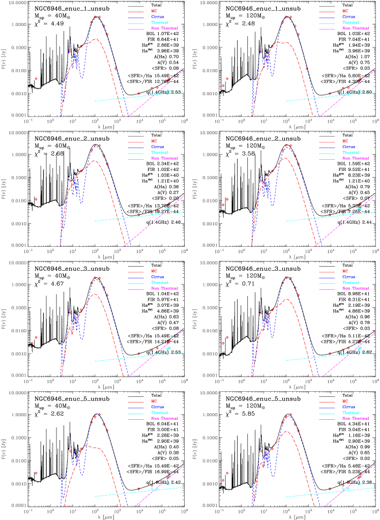
Figure 9: GRASIL best fit SEDs for the extra-nuclear regions of NGC 6946 (red diamonds) for upper mass limit of 40 (left panels) and 120 $\rm{M}_{\sun}$(right panels). To test our radio decomposition, we over-plotted on top our thermal radio component (dotted-dashed cyan lines) the local background subtracted radio data flux (cyan diamonds) by Murphy et al. (2011).

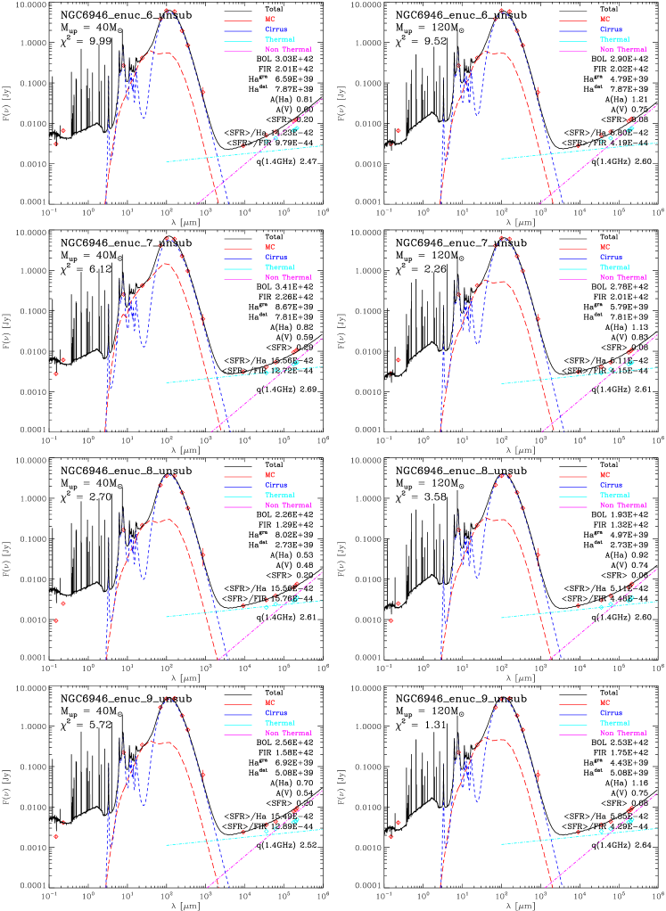
Figure 10: continued

For all regions the observed IR SED can be fairly well reproduced by using either of the IMF upper mass limits. In general, the value of $q_{1.4}$ is found to lie between 2.5 and 2.6. This is about 0.2 dex larger than the value observed in the normal star-forming galaxy M100 ($q_{1.4}$  =  2.35) implying that, in these star-forming regions, the ratio between radio and FIR luminosity is about a factor 1.6 lower than in the normal star-forming galaxy M100. The estimated young starburst ages support the notion that this is due to a lack of non-thermal radio emission as predicted by the original models by B02. This is also evident from the radio slope which is found to be flatter than the value observed in the normal star-forming galaxy ($\alpha\simeq$- 0.8). It is worth reminding here that we adopted the calibration ($E^{NT}_{1.49}$) of non-thermal radio luminosity obtained from the fits to M100. We note also that since the radio emission is dominated by the thermal component, which has no free parameters, the SFR in these regions is very well determined by the 33 GHz point, modulo the IMF. Another characteristics of the fits is the difficulty of reproducing the UV data, in spite of a fairly well fit in all the other bands from mid-IR to radio bands. In particular the runs with $M_{up}=40~{}M\sun$ tend to show larger UV fluxes than the corresponding cases made with $M_{up}=120~{}M\sun$, which is against what could be expected from the dependence of the UV luminosity on the IMF. This can be noted in Figure 9 where we see that adopting $M_{up}~{}=~{}120~{}M\sun$ we either reproduce or underpredic the far-UV data while, adopting $M_{up}~{}=~{}40~{}M\sun$, we either reproduce or overpredict them. At the same time, the average SFR in the models with $M_{up}~{}=~{}40~{}M\sun$ is about two to three times larger than that obtained with the models that adopt $M_{up}~{}=~{}120~{}M\sun$. This is in evident contrast with what we have found in the fits of normal galaxies where we see that the SFR, obtained with different values of $M_{up}$, differ by 20 per cent at maximum and it is a consequence of the young age of such star bursting regions, where the bolometric luminosity is dominated by the most massive stars. Finally, the attenuation in the models with $M_{up}~{}=~{}40~{}M\sun$ is always lower than that obtained with the models adopting $M_{up}~{}=~{}120~{}M\sun$. As the non-thermal radio emission starts about 7 Myr after the beginning of the burst of star formation (see Figure 5), we have the opportunity to perform an accurate decomposition of the radio flux into thermal and non thermal components. We present in Table 4 the thermal fraction resulting from this decomposition and we show the two radio components in Figure 9. To show the quality of our decomposition, we also show in Figure 9 and only for the case with $M_{up}~{}=~{}120~{}M\sun$, the background subtracted radio data fluxes (cyan diamonds) by Murphy et al. (2011). In the next section, we will discuss the SFR calibrations derived using our best fit model of the galaxies studied in this work.

Table 1: GRASIL best fit parameters (for upper mass limits of 40 and 120$~{}\rm{M}\sun$) for the modelled SEDs of M100 and NGC 6956 SF regions.

ID	$t_{gal}/t_{sb}$	$t_{esc}$	$\beta$	$\tau_{1}$	$f_{mol}$
	(Gyr/Myr)	(Myr)
(1)	(2)	(3)	(4)	(5)	(6)
			$M_{up}$	= 40 M☉
M100	12.0	2.5	2.0	12.0	0.10
NGC 6946_1	8.0	1.0	2.1	9.07	0.30
NGC 6946_2	9.0	0.5	1.7	12.00	0.05
NGC 6946_3	8.0	1.0	2.0	24.48	0.20
NGC 6946_5	8.0	0.3	2.0	4.15	0.25
NGC 6946_6	12.0	1.2	2.2	5.33	0.40
NGC 6946_7	7.0	1.0	2.1	14.81	0.30
NGC 6946_8	7.0	0.6	2.1	6.12	0.22
NGC 6946_9	8.0	1.0	2.1	5.33	0.30
			$M_{up}$	= 120 M☉
M100	12.0	0.9	2.0	14.81	0.10
NGC 6946_1	11.0	0.6	2.2	5.33	0.12
NGC 6946_2	11.0	1.0	1.7	16.60	0.15
NGC 6946_3	8.0	0.9	2.2	12.00	0.14
NGC 6946_5	18.0	1.0	1.8	18.75	0.50
NGC 6946_6	11.0	0.7	2.2	5.33	0.12
NGC 6946_7	8.0	1.0	2.2	5.33	0.16
NGC 6946_8	8.0	0.9	2.2	5.33	0.12
NGC 6946_9	9.0	0.6	2.2	5.33	0.12

Column (2) gives the age of the galaxy ($t_{gal}$) in Gyr for the normal star-forming galaxy M100 and the age of the burst ($t_{sb}$) in Myr for the NGC 6946 star-bursting regions. Parameters in other columns are as described in text.

5 Discussion

In this section we discuss the results obtained from the best fits of the SEDs of M100 and the extra-nuclear regions of NGC 6946. We begin with the SFR calibrations obtained with the new SSPs and then discuss the impact of the newly added emission line prediction on the resulting attenuation.

5.1 Star formation rate calibrations from GRASIL best fits

We first show in Table 3 the luminosities of the best fit models in the selected photometric bands, from the UV to radio wavelengths. The upper panel refers to the results obtained adopting $M_{up}~{}=~{}40~{}M_{\sun}$ while, the lower panel refers to those obtained with $M_{up}~{}=~{}120~{}M_{\sun}$. The FIR luminosity in column 11 was obtained by integrating the IR specific luminosity from 3 to 1000 $\micron$. We also show the predicted intrinsic (suffix ^int) and transmitted (suffix ^tra) intensities of the H$\beta$ and H$\alpha$ emission lines, the value of $q_{1.4}$ (Equation 1), the relative contribution to the 3 - 1000 $\micron$ FIR luminosity by the molecular clouds component and by the cirrus component, and the ratio between the 3 - 1000 $\micron$ FIR and the bolometric luminosity. In the columns of radio luminosities, we enclose in parenthesis the fractional contribution of the thermal radio component to the total radio emission, derived from the models.

Effects of Mup
By construction, i.e. since we are discussing best fits SEDs, the predicted luminosities obtained with the two different $M_{up}$ are very similar, but for those in the emission lines and in the UV bands. These are the most difficult to model because they are the most sensitive to the attenuation. This is not the only reason however, because even the intrinsic H$\alpha$ and H$\beta$ luminosity differs by a significant factor in the two $M_{up}$ cases. Indeed, in the two cases the ionizing photon flux (and the far and near-UV) differ much more than the corresponding bolometric luminosities. Said in another way, one may be able to obtain the same bolometric flux with two different IMF upper limits but the amount of ionizing photons may be significantly different, and this mainly affect the intensity of the recombination lines and the free-free radio emission. Note however that the 33 GHz luminosity does not show the same strong dependence on the adopted Mup as that shown by the recombination lines, and this is likely due to the fact that a non negligible contribution of the non-thermal luminosity is present even at this high radio frequency, which should be larger in the case of lower $M_{up}$. The best fit transmitted intensities of the H$\alpha$ emission lines are compared with the observed ones in Figure 11, for both cases of $M_{up}$. We do not include M100 in this plot to better show the case of the star-forming regions. The solid line indicates the one-to-one correlation. We see that, in the case of extra-nuclear regions, the predicted values of the case with $M_{up}~{}=~{}40~{}\rm{M}_{\sun}$ are larger than those of the case with $M_{up}~{}=~{}120~{}\rm{M}_{\sun}$.

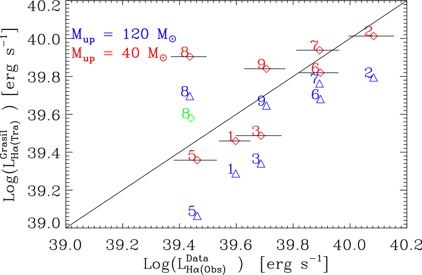
Figure 11: Comparisons between our model’s transmitted intensities of the H$\alpha$ emission lines with the observed ones, for $M_{up}~{}=~{}40M_{\sun}$ (red daimonds) and $M_{up}~{}=~{}120$$M_{\sun}$ (blue triangles) cases. The solid line indicates the one-to-one correlation whereas the horizontal lines indicate the errors in the observed H$\alpha$ line. The green daimond indicates the case with $M_{up}~{}=~{}350~{}\rm{M}_{\sun}$ for the extra-nuclear region 8.

In general our best fit models are able to reproduce the observed values with an accuracy of about 50 per cent. Looking to individual regions, we see that regions $\sharp$1 ,$\sharp$2, $\sharp$3, $\sharp$5, $\sharp$6 are compatible with $M_{up}=40~{}\rm{M}_{\sun}$ while, for regions $\sharp$9 and $\sharp$7, a larger value of $M_{up}$ seems suggested, up to $M_{up}~{}=~{}120~{}\rm{M}_{\sun}$. From the figure it also appears that, in order to fit region $\sharp$8, an even higher IMF upper mass limit (see the green daimond in Figure 11 for the case of $M_{up}~{}=~{}350~{}\rm{M}_{\sun}$) should be used. Furhermore, we note that the in all cases where we are able to reproduce the observed H$\alpha$ emission we are also able to reproduce fairly well the observed FUV luminosity, which is also strictly related to the intrinsic ionizing photon flux. On the contrary the NUV flux is not well reproduced by our models, likely indicating that its origin is not strictly related to the star formation process. Since all model reproduce the observed bolometric luminosity and, in particular, the 24 $\micron$ and the 33 GHz data, we conclude that, by combining in a consistent way this relevant information, it is possible to obtain a fairly robust estimate of the upper mass limit of the IMF . Indeed we stress that the FIR luminosity and those at H$\alpha$, 33 GHz and 24 $\micron$ bracket, on one side, the intrinsic ionizing photon flux and, on the other, the attenuation and re-emission by molecular clouds where the stars reside during their initial phase, which are the most sensitive to the fractional contribution of the most massive stars.

As far as the prototype normal galaxy M100 is concerned, we remind that the observed H$\alpha$ luminosity was matched by the model with $M_{up}~{}=~{}40~{}M_{\sun}$. It is important, at this stage, to remind that these conclusions should be taken with care because the current SSP adopted do not account for binary evolution. Indeed it is known that binary evolution can produce more ionizing photons at later stages than single star evolution, because of the loss of the envelope by binary interaction (Wofford et al., 2016). In particular we may say that regions $\sharp$1 ,$\sharp$2, $\sharp$3, $\sharp$5, $\sharp$6 may be reproduced fairly well without invoking a high $M_{up}$ and/or significant effects by binary evolution. The latter effect could instead explain the location of region number $\sharp$8 that cannot be reproduced even with $M_{up}~{}=~{}350~{}M_{\sun}$, as indicated by the green diamond in Figure 12). This effect, which add a new dimension to the problem, is under study in PARSEC and it will be included in the nearest future.

The q ratio.
The second thing that we note by inspecting Table 3 is that the value of the q_1.4 does not significantly depend on the upper limit of the IMF. This is because a significant fraction of both the bolometric luminosity and the radio luminosity are contributed by stars less massive than M = $40~{}M_{\sun}$. Indeed after a few Myr, the upper mass of the SSP is already significantly lower than M = $120~{}M_{\sun}$. Furthermore, the q_1.4 ratio is generally higher in the extranuclear regions of NGC 6946 than in the normal SF galaxy M100, by a factor of $\simeq$1.4. We remind that in our model, CCSNs, responsible for the non thermal emission, are produced only by the mass range $10~{}M_{\sun}$ $\leq$ M$\leq$  $30~{}M_{\sun}$ and the individual star-bursting regions have an age which is younger than the threshold for CCSN production. Thus they did not yet reach a stationary equilibrium for non-thermal radio emission and not only their radio slopes appear flatter but also their q_1.4 are higher than that of normal star-forming galaxies B02.

The SFR calibration.
Using the luminosity in the different bands, as presented in Table 3, and the average SFR obtained from the GRASIL fits, we show in Table 4, the corresponding SFR calibrations C(b) = SFR/L(b), where b indicates the band. The average SFR is derived by considering the last 100 Myr time interval for the normal star-forming galaxy M100, and the age of the burst in the star-forming regions of NGC 6946, which is shown in column 16 of Table 4 for the NGC 6946 extranuclear regions. This choice is suggested by the fact that within an entire galaxy, the star-forming regions distribute continuously with time while, this is obviously not the case for individual regions. The average SFR ($\rm{M}_{\sun}\;\rm{yr}^{-1}$) so computed is shown in the second column of Table 4. These calibrations are directly obtained by GRASIL. For sake of comparison, we also add, in Table 4, some calibrations that can be obtained by using the un-attenuated fluxes derived from GRASIL best fit models, either directly or by using the analytical relations obtained by means of the SSPs. These are useful to compare the differences between the SFR derived from a panchromatic fit that realistically account for ISM processes to analytical fits made with SSP fluxes. For example, the FUV, H$\beta$ and H$\alpha$ values shown in column 3, 4 and 6, refer to the calibrations obtained by dividing the average SFR by the corresponding un-attenuated intrinsic fluxes of the models, listed in Table 3. For H$\beta$ and H$\alpha$ we also show, in columns 5 and 7, the values obtained by inserting their corresponding intrinsic fluxes in the analytical calibrations obtained from simple SSPs models, Equations 40 and 39 respectively. For the 33 GHz radio emission, we add in column 15, the value of the calibration C(33)^SSP = SFR/L(33 GHz), directly derived from the SSP models (Equation 38). The last rows in the first and second sections, indicated by $<NGC~{}6946>$, show the median values of all SFR calibrations derived from the star-bursting regions of NGC 6946. In the third section we collect some common SFR calibrations from the literature, with the corresponding bibliographic sources given in the caption.

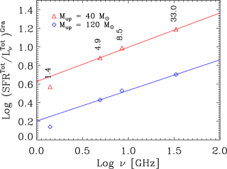
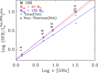
Figure 12: Left panel: SFR calibration constants C($\nu$), in units of $\rm{M}_{\sun}\rm{yr}^{-1}10^{28}\rm{erg}^{-1}\;\rm{s}\;\rm{Hz}$, at $\nu$ = 1.4, 4.9, 8.5 and 33.0$\rm{GHz}$ (Table 4), for the star-bursting regions and using the total radio emission. Triangles and daimonds indicate cases of $M_{up}~{}=~{}40~{}\rm{M}_{\sun}$ and $M_{up}~{}=~{}120~{}\rm{M}_{\sun}$ respectively. Right panel: The same as in the left panel but for M 100 and using both the total radio (crosses) and non-thermal radio emission (xs). In both panels, all red symbols and lines indicate cases of $M_{up}~{}=~{}40~{}\rm{M}_{\sun}$ and blue symbols and lines cases of $M_{up}~{}=~{}120~{}\rm{M}_{\sun}$. Also all lines represent least-square fits.

In Figure 12 we plot the calibration constants C($\nu$) at $\nu$ = 1.4, 4.9, 8.5 and 33.0 $\rm{GHz}$, in units of $\rm{M}_{\sun}\rm{Yr}^{-1}10^{28}\rm{erg}^{-1}\;\rm{s}\rm{Hz}$, against the corresponding radio frequencies, for both the star-bursting regions (left panel) and M100 (right panel) and for both cases of $M_{up}$. The relations (in logarithmic units) are almost linear above 1.4 GHz, and we show the best fit regressions as solid lines. Concerning the dependence on M_up, there is a clear difference between the starburst and the normal star formation regime in the sense that, in the former case the constant is about a factor of three larger independently from the frequency. Again this effect is due to the young age of the starburst regions coupled with the dependence of the thermal radio emission on M_up. Indeed for the normal SFR regime, the dependence on M_up becomes significant only at high frequencies, where the thermal emission start dominating. From the fits we derive the following general relations between SFR (in $\rm{M}_{\sun}\rm{yr}^{-1}$) and radio luminosity (in $\rm{erg}\;\rm{s}^{-1}\rm{Hz}^{-1}$). For Star-bursting regions, with average metallicity $\sim$ 0.006, we have at any frequency between 1.4 $\rm{GHz}$ and 33 $\rm{GHz}$, to better than 10 per cent,

$$\rm{log}(\frac{SFR}{L\nu})^{tot}~{}=~{}0.43\ \rm{log}(\nu)-0.96\ \rm{log}(\frac{M_{up}}{120})-27.91$$ (22)

while, for the normal star-forming galaxy, M100, with slightly more than solar metallicity, we have for the total radio emission

$$\rm{log}(\frac{SFR}{L\nu})^{tot}~{}=~{}0.73\ \rm{log}(\nu)-0.16\ \rm{log}(\frac{M_{up}}{120})-28.31$$ (23)

and for the non-thermal radio emission, we have

$$\rm{log}(\frac{SFR}{L\nu})^{nth}~{}=~{}0.58\ \rm{log}(\nu)-0.43\ \rm{log}(\frac{M_{up}}{120})-28.33$$ (24)

Relations similar to Equations 22,  23 and  24 above were provided by Murphy et al. (2011), assuming Kroupa IMF (with $M_{up}=100~{}\rm{M}_{\sun}$ ), solar metallicity and a constant SFR over a timescale of 100 Myr. For total radio emission

$$\left(\frac{SFR}{L\nu}\right)^{tot}_{Mur}=10^{-27}\left(2.18\nu^{-0.1}(\frac{T_{e}}{10^{4}})^{0.45}+15.1\nu^{-0.85}\right)^{-1}$$ (25)

and for non-thermal radio emission

$$\left(\frac{SFR}{L\nu}\right)^{nth}_{Mur}=10^{-27}(6.64\times 10^{-29}\nu^{0.85})$$ (26)

These relations are in between our relations in 22 and 23, running only $\lesssim$ 20 per cent lower than our one for normal star-forming galaxies, below 33 GHz. However at frequencies higher than 33 GHz the difference grows rapidly and at 100 GHz our values are $\sim$40 per cent and $\sim$200 per cent higher than that of Murphy et al. (2011) for starburst and normal galaxies, respectively. Interestingly, the relation derived by Schmitt et al. (2006) with Starburst99, assuming a Salpeter IMF (with $M_{up}~{}=~{}100~{}\rm{M}_{\sun}$), solar metallicity and a continuous SFR of 1 $\rm{M}_{\sun}\;yr^{-1}$

$$\left(\frac{SFR}{L\nu}\right)^{tot}_{Sch}~{}=~{}10^{-27}(8.55\nu^{-0.8}+1.6\nu^{-0.1})$$ (27)

agrees well with our relations in 22 and 23 at frequencies from about 33 GHz to 100 GHz. Above 100 GHz the dust emission contribution becomes dominant.

It is interesting to compare the GRASIL calibration at 33 GHz with that derived from the SSP models (Equation 38), i.e. columns 14 and column 15 in Table 4. The values show some discrepancies, especially for normal galaxies. However we remind that the values in column 15 refer to free-free emission alone while the 33 GHz flux in column 14 may include a non negligible contribution by synchrotron emission. If we take this contamination into account, using the percentage contribution of the thermal radio component enclosed in parenthesis, the corrected values of column 14 are in fair agreement with those predicted by Equation 38. This is expected because, at these wavelengths, attenuation, including also the free-free one (Vega et al., 2008), should not be important. The above overall agreement indicate a surprising robustness of the radio calibration, irrespective of the differences in the underlying models. This will be particularly important for the high redshift galaxies especially in their early evolutionary phases.

As a further comparison, we provide at the bottom of Table 4 other SFR calibrations taken from the literature. We remind the reader that, in this work, we adopt a Kennicutt (1983) IMF and a typical time-scale for averaging the SFR rate of 100 Myr for normal galaxies and equal to the age of the starburst in the extra-nuclear star bursting regions. The details on the parameters adopted by different authors may be found in the quoted papers.

5.2 Dust attenuation properties

It has been already shown in (Silva et al., 1998; Granato et al., 2000) that the attenuation is the result of the interplay between the extinction properties of dust grains and the distribution between dust and stars in space and in time. Further discussion can also be found in (Charlot & Fall, 2000; Panuzzo et al., 2003). We now investigate the properties of the attenuation curves of the galaxies studied here, with particular interest to understand its dependence on the galaxy type, i.e. starburst vs. normal regime, and also the effects of using different parameters in the analysis, such as M_up in the IMF.

We first show in Figure 13, the attenuation curves, A_λ/A_V, of M100 (green solid line) and of the NGC 6946 extra-nuclear regions studied in this work (black solid lines). They are simply derived by comparing the transmitted galaxy flux to the intrinsic one, as a function of the wavelength. The top panel refers to the case of $M_{up}~{}=~{}40~{}\rm{M}_{\sun}$ while the case with $M_{up}~{}=~{}120~{}\rm{M}_{\sun}$ is shown in the bottom panel.

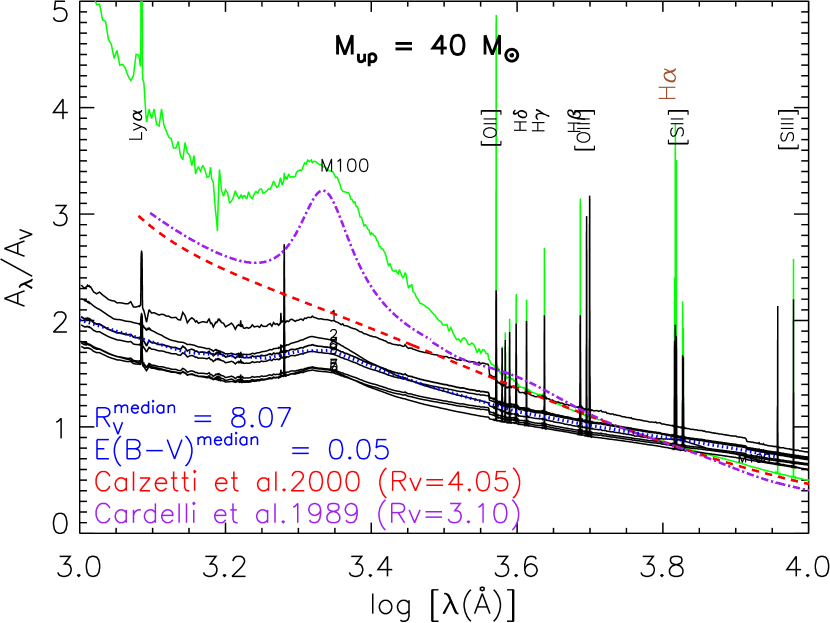
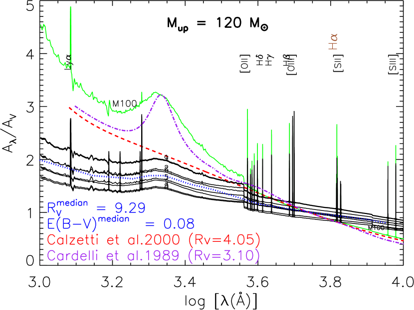
Figure 13: Attenuation curves, A_λ/A_V, for M100 and NGC 6946 extra-nuclear regions, for the cases of $M_{up}~{}=~{}40$ (top panel) and $M_{up}~{}=~{}120~{}\rm{M}_{\sun}$ (bottom panel). The black solid lines are the attenuations curve of the eight regions of NGC 6946 while the dotted blue line represents the median of these curves. The median values of $R_{V}$ and ${E(B-V)}$ for the star-forming regions are also given in the labels. The green line is the attenuations curve of M100. For comparison purposes, we added the attenuation curves of Calzetti et al. (2000) (red dashed line) and Cardelli, Clayton & Mathis (1989) (purple dotted-dashed line) The later attenuation seems to agree very well with that of M100 at wavelengths above $\sim$ 4000 Å.

The dotted blue lines represent the median curve of the NGC 6946 extra-nuclear regions obtained by sampling the curves of individual regions at selected wavelengths. The median values of the quantities $E(B-V)$ and R_V = A_V/E(B-V) for the star-bursting regions are also given in the labels. We have also labelled some prominent emission lines ($H\alpha$ line is in brown). For comparison purposes, we added the attenuation curves of Calzetti et al. (2000) (red dashed lines) and Cardelli, Clayton & Mathis (1989) (purple dotted-dashed lines). We also collect in Columns (2 - 9) of Table 5 the attenuation in H$\alpha$, H$\beta$, in the FUV (0.16 $\micron$) and NUV (0.20 $\micron$), in the B-band(0.45 $\micron$), and in the interpolated continuum at H$\beta$ (named A48), in the V-band(0.55 $\micron$) and in the interpolated continuum at H$\alpha$ (named A65). Columns 10 and 11 give the optical depth of the molecular cloud at 1 $\micron$ derived from GRASIL and the $R_{V}$ ratio, respectively. In Column 12 we show the difference A₄₈-A₆₅ which corresponds to $E(48-65)$. Using the Balmer decrement method for the $H\beta$ and $H\alpha$ lines, we also obtained the same quantity, $E(H\beta-H\alpha)$:

$$E(H\beta-H\alpha)=1.086\left({\rm ln}(\frac{H\beta^{int}}{H\alpha^{int}})-{\rm ln}(\frac{H\beta^{tra}}{H\alpha^{tra}})\right)$$ (28)

and show its value in Column 13. We assume an intrinsic line intensity ratio, $(H\alpha^{int}/H\beta^{int})$ = 2.86, which is valid for $T_{e}$ =10,000 K (Hummer & Storey, 1987). Column 14 gives the escape time of young stars from their birth cloud in Myr. Column 15 gives the FIR flux in $\rm{ergs}\,\rm{s}^{-1}\,\rm{cm}^{-2}$ in the 40 - 120 $\micron$ interval derived using the 60 and 120 $\micron$ fluxes (Helou et al., 1988).

Several points can be noted by inspection of Figure 13 and Table 5. First of all, we see that, while in normal galaxies the attenuation in the lines is significantly higher than that in the surrounding continuum, (a factor of 4 on average for M100), this is not true for the star bursting regions where this factor is not more than 1.3. The fact that the attenuation in the lines is significantly higher than that in the surrounding continuum is well known and it is a manifestation that young stars are more dust enshrouded than older stars. However, in the case of the star-bursting regions the underlying continuum is essentially produced by the same stellar populations, with a small contribution from the older populations, so that the attenuation in the lines is not much different from that in the continuum. To get more insights from the models we compare the characteristic R values in the lines and in the nearby continuum. We see that for star-forming galaxies, R_Hα = A${}_{H\alpha}/($A_Hβ-A_Hα) is much larger than the value obtained in the corresponding interpolated underlying continuum regions (R${}_{65}=A_{65}/(A_{48}-A_{65}$). For example, for M100, R_Hα = 16(10) while R₆₅ = 4(4), for M_up = 40(120) M_☉. In the starburst regions, R_Hα and R₆₅ have similar values between 6 and 10. The high values so determined for R_Hα would suggest a high neutral absorption in these objects but this is not the case because we have not modified the grain size distribution which, by default in GRASIL is the one of the Galactic ISM. We also see that in M100, R₆₅, in the continuum, has a value of $\sim$3, compatible with the common extinction laws provided in literature (Calzetti et al., 2000; Cardelli, Clayton & Mathis, 1989). Instead this effect is due to the fact that the attenuation within molecular clouds is so high (see the values of $\tau_{1\micron}$ in Table 5) that the emission of young stars is almost completely absorbed, until they escape from the clouds. This effect mimics the neutral absorption. This effect is enhanced for the emission lines because they are generated only by stars younger than about 6 Myr, so that the fraction of line flux absorbed by molecular clouds with respect to the total one, is even higher. Adopting a $t_{esc}$ larger than 7 Myr will erase line emission in our model, irrespective of the galaxy types considered here. A major consequence of the age selective attenuation described above is that it leads to wrong estimates of the attenuation in the line emission, if one uses methods involving attenuation-affected observables, like the Balmer decrement method. A more accurate method to estimate the intrinsic H$\alpha$ luminosity (hence the H$\alpha$ attenuation) is by using the 33 GHz and 24 $\micron$ luminosities, since they are optimal tracers of the radiation emitted by the most massive. Adopting a median value of 78.5 per cent as the percentage contribution of the thermal radio component in young star-bursts, we first obtain the thermal radio emission component of our model’s 33 GHz total radio emission luminosity. Using the analytical relation given in Equation 2 (T_e and gaunt factors used here are as given in Equations 34 and  3 respectively), we derive the number of ionizing photons corresponding to this luminosity. With Equation 35, we then estimate the corresponding intrinsic H$\alpha$ luminosity. A plot of the estimated intrinsic H$\alpha$ luminosity (in ${\rm erg}\;{\rm s}^{-1}$) against our model’s 33 GHz thermal radio luminosity (L₃₃ in ${\rm erg}\;{\rm s}^{-1}{\rm Hz}^{-1}$) is presented in Figure 14. We added in this figure also the normal SF galaxy M100, with an average thermal fraction of 16.0 per cent(42.0 per cent) for M_up = 40 $\rm{M}_{\sun}$(M_up = 120 $\rm{M}_{\sun}$), respectively. The fitting relation (solid line) considering only the star bursting regions for both cases of M_up, is given by

$${\rm log}({\rm L_{H\alpha}^{int}})={\rm log}(0.785{\rm L(33)})+14.10$$ (29)

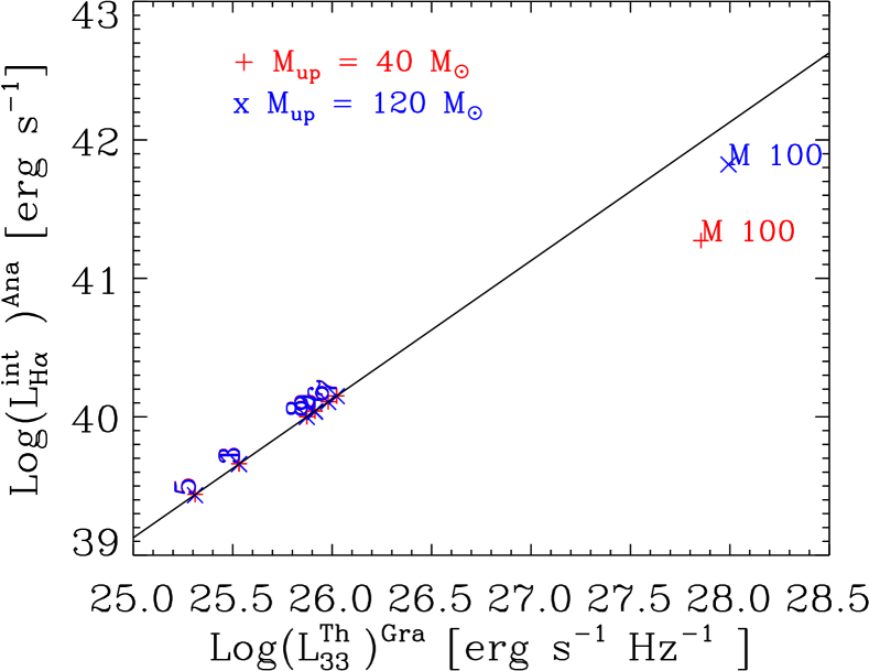
Figure 14: Plot of our model’s 33 GHz thermal radio luminosity against the intrinsic H$\alpha$ luminosity. Solid line represents linear fit for the star-bursting regions. The H$\alpha$ luminosity here is derived from the thermal radio luminosity using Equations 2 and 35. We adopted a median thermal fraction of 78.5 per cent in estimating the thermal radio component of the 33 GHz total radio luminosity. We also added in this plot the M100 which has an average thermal fraction of 16.0 per cent(42.0 per cent) for M_up  =  40 $\rm{M}_{\sun}$(M_up  =  120 $\rm{M}_{\sun}$).

luminosity (L33 in erg s?1Hz?1) is presented in Figure 12.

The corresponding attenuation at H$\alpha$ can be obtained by using the intrinsic value provided by equation 29

$${\rm A_{H\alpha}}=-2.5{\rm log}\left(\frac{H\alpha^{obs}}{0.785{\rm L_{33}}}\right)+35.25$$ (30)

As mentioned earlier, this attenuation is larger than the one that can be obtained with the Balmer decrement method because the latter might not accounts for the strong obscuration in the early life of massive stars (see Table 5). Thus, in presence of an estimate of the radio flux at 33 GHz, Equation 30 should be preferred for young starbursts. A similar relation, though with somewhat larger scatter, can be obtained for the 24 ${\micron}$ flux, which is shown in Figure 15. The relation between the model’s intrinsic H$\alpha$ (in ${\rm erg}\;{\rm s}^{-1}$) and 24 $\micron$ luminositiy, L₂₄ = $\lambda$L_λ in ${\rm erg}\;{\rm s}^{-1}$, is

$${\rm log}({\rm L_{H\alpha}^{int}})=0.59{\rm log}({\rm L_{24}})+15.73$$ (31)

almost independently from M_up. Correspondingly, the derived attenuation in H$\alpha$ is

$${\rm A_{H\alpha}}=-2.5{\rm log}\left(\frac{H\alpha^{obs}}{1.48\rm L_{24}}\right)+39.33$$ (32)

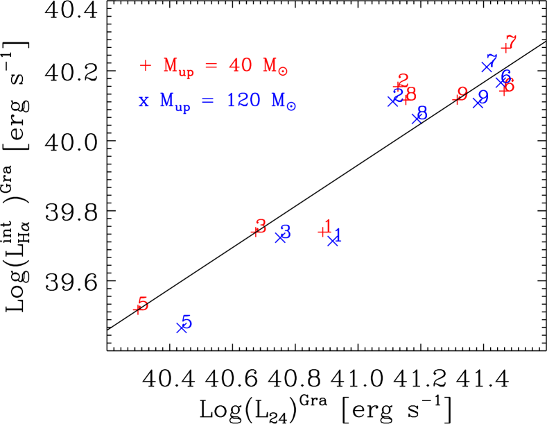
Figure 15: Plot of the 24 $\micron$ luminosity against the intrinsic H$\alpha$ luminosity, both extracted directly from our best-fit models. Solid line represents linear fit. We excluded M100 in this plot so as to better represent the star-bursting regions.

It is also interesting to provide a relation between the attenuation at 1600 Å (Column 4 of Table 5) and the ratio of FIR (Column 11 of Table 3) to F${}_{1600}^{tra}$ (Column 3 of Table 3). The plot is shown in Figure 16, along with the linear fitting relation obtained for the star-bursting regions (solid line), for both M_up cases.

$$A_{1600}~{}=~{}1.209{\rm log}\left(\frac{FIR}{F_{1600}^{obs}}\ \right)+0.254$$ (33)

We note that the normal galaxy M100 is out from the relation. This may likely be due to the non negligible contribution to the FIR intermediate age stellar populations that are not contributing to the far UV.

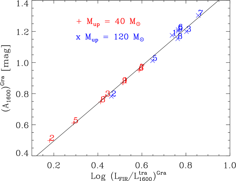
Figure 16: Plot of attenuation at 1600 Å against the ratio, $FIR/F_{1600}$, both extracted from our best-fit models. The solid black line represents our linear fit as given in Equation 33. The red crosses and blue ’X’s indicate M${}_{up}~{}=~{}40$ and 120 $\rm{M}_{\sun}$ cases respectively.

6 Conclusions

In this paper we have used the recent PARSEC tracks to compute the integrated stellar light, the ionizing photon budget and the supernova rates predicted by young SSP models for different IMF upper mass limits. The SSPs spans a wide range in metallicities, from 0.0001 to 0.04 and initial masses ranging from 0.1 to 350M$\sun$. In building the integrated spectra, we have adopted the spectral library compiled by Chen et al. (2015). This library is a result of homogenising different sets of libraries through a process fully described in Girardi et al. (2002) and Chen et al. (2014). Using this integrated spectra in the photoionization code CLOUDY, we have also calculated and included in the integrated spectra the nebular continum and the intensities of some selected emission lines. With the new SSPs we can then be able to predict the panchromatic spectrum and the main recombination lines of star-forming galaxies of any type, with GRASIL.

We made also two major revisions in the radio emission model. First, we revisited the relation between free-free radio emission, number of ionizing photons and radio frequency and came up with a relation that (a) takes into account the full dependence of the electron temperature on the metallicity and the effect of considering different IMF upper mass limits and (b) incorporated a more accurate gaunt factor term. The free-free radio emission shows a significant variation with metallicity and IMF upper mass limit, decreasing by a factor of about 3 when Z increases from 0.0001 to 0.02 and inceasing by more than an order of of magnitude when the mass limit is increased from 40 to 350 $M\sun$, at constant total mass. These differences cannot be negelected, especially when calibrating SFRs using tracers that depend strongly on the ionizing photon budget. Hence, the corresponding SFR calibrations (H$\alpha$, H$\beta$ and thermal radio emission) take into account this dependence on metallicity and IMF upper limits.

Second, we revised the non-thermal radio emission model originally described by B02, taking into account recent advances in the CCSN explosion mechanisms which indicates a range of stellar masses where the stars fail to explode, the so called Failed SNe. We adopt a threshold value of 30 M$\sun$, above which stars do not produce non-thermal radio emission. This has two immediate effects: (a) the beginning of the non-thermal radio emission is delayed by about 7 Myr, $\sim$ the lifetime of a 30 M$\sun$ star; (b) the non-thermal radio emission is independent from the IMF upper mass limit as long as it is above 30 M$\sun$. It is also assumed that pair-instability SNe, discussed by Slemer et al. (2017) do not produce synchrotron radiation.

With these revisions in the new SSPs and in the radio emission model, there is the need to check some parameters of the GRASIL code. We first re-calibrate the proportionality constant between the supernova rate and the corresponding non-thermal radio luminosity, $E_{1.49}^{NT}$), using one of the best-sampled nearby normal star-forming galaxy, M100. We are able to reproduce very well the far-UV to radio SED of this galaxy, for IMF upper mass limits of 40 $M_{\sun}$ and 120 $M_{\sun}$, with an average $q_{1.4}$ of 2.42. We obtain a value of $E_{1.49}^{NT}$ = 1.94 which is larger than that obtained previously by B02 by a factor of 1.35, but it is similar to that obtained by Vega et al. (2005). We find that using M${}_{up}~{}=~{}350~{}\rm{M}_{\sun}$ produces a thermal radio emission that significantly exceeds the observed one. This excess thermal radio emission cannot be cured by varying any other parameter in the fit. This result suggests that, for a normal star-forming galaxy, it is difficult to have an average IMF extending up to such high initial masses. What depends strongly on the upper mass limit of the IMF is the number of ionizing photons, which beqars on the intensity of the recombination lines and on the thermal radio emission. Indeed, in spite of being able to reproduce the FIR and 1.4 GHz radio emission, the model that adopts M_up = 120 $M_{\sun}$ over predicts the H$\alpha$ emission by a factor of about three while, in the case of M_up = 40 $M_{\sun}$, the discrepancy is only of a few percent.

We then check the new thermal radio emission model against the well studied thermal radio dominated star-forming regions in NGC 6946. Even in this case we are able to reproduce very well the observed SEDs from NIR to radio wavelengths for both cases of the IMF upper mass limits. In fitting the SEDs of these thermal radio-dominanted star-bursting regions, we adopt the value of $E_{1.49}^{NT}$ resulting from the non-thermal radio calibration with the normal star-forming galaxy M100. The estimated values of the $q_{1.4}$ ratio in these regions lie between 2.5 and 2.6, implying a relatively lower non-thermal emission than in normal star-forming galaxies. The additional evidence of flatter radio slopes supports the notion that there is lack of the non-thermal emission as predicted by the original non-thermal radio emission models by B02. The resulting ages of the bursts, range from 7 to 12 Myr, confirming that these observations can be used to determine the star-burst ages. The fit obtained with the two IMF upper mass limits exhibit interesting differences, in particular in the predicted H$\alpha$ and UV luminosities which are the most sensitive to the IMF and to dust attenuations. We show that, by combining information from the FIR, 24 $\micron$, 33 GHz and H$\alpha$, we can determine the preferred value for M_up. This is the first time, to the best of our knowledge, that the IMF upper mass limit can be consistently determined. However, for region $\sharp$8 we cannot reproduce the observed H$\alpha$ flux even with M${}_{up}~{}=~{}350~{}\rm{M}_{\sun}$. This could be a case where binary evolution, which is known to produce an excess of ionizing photons due to the loss of the envelope of massive stars by binary interaction, may be required.

With luminosities and averaged SFR extracted from our best fit models (Table 3), we derive SFR calibrations in different bands for both normal galaxies and star-burst regions (Table 4). Since thermal radio emission and that in the recombination lines depend strongly on the upper mass limit of the IMF, we provide multiple regression fitting relations with M_up and metallicity (e.g. Equations 38, 39 40).

Finally, exploiting the realistic treatment of dust performed by GRASIL, we investigate the properties of the attenuation curves of the galaxies studied in this work with the aim of understanding their dependence on the galaxy type. We find that, while in the normal SF galaxy M100 the attenuation in the lines is significantly higher than that in the surrounding continuum, for the star bursting regions of NGC 6946 the two attenuations are similar. A common property is that the predicted R values obtained for the ${H\alpha}$ line is large, mimicking a significant neutral absorption. For star bursting regions, large values are found also for the continuum while, in the case of M100, the R value of the continuum is normal. Large R values have been found in high redshift star-forming galaxies by Fan et al. (2014), using a completely different population synthesis tool. A major disturbing consequence of the age selective attenuation, which could not be revealed in a foreground screen model, is that it leads to wrong estimates of attenuation when using methods involving observed line fluxes, like the Balmer decrement. Of course, more accurate methods are those that combine UV or line fluxes with fluxes that are not affected by attenuation, such as the well known relation between the FUV (at 1600 Å) attenuation and the flux ratio ratio, FIR/F₁₆₀₀. For the star-forming regions we revisit the former relation (Equation 33) and we provide new relations between the H$\alpha$ attenuation and the observed H$\alpha$and 24 $\micron$ (Equation 30) or 33 GHz (Equation 32) fluxes. The above mentioned relations, which we show to be almost independent from M_up, can be extremely useful in estimating the attenuations in young high redshift galaxies. For this purpose we are working on a larger galaxy sample to increase the statistical significance of our results.

Appendix A Variation of electron temperature and the constants, $C_{2}$ and $C_{3}$, with IMF Upper mass limits and metallicity

Table 2: Calibration constants, $C_{2}$ and $C_{3}$, for different metallicities and upper mass limits.

$\rm{Z}$	$IQ(H)$	$C_{2}$	$T_{e}$	$C_{3}$
	$(10^{54}$	$(10^{-54})$	$(10^{4})$	$(10^{26})$
(1)	(2)	(3)	(4)	(5)
$M_{up}~{}=~{}40~{}\rm{M}_{\sun}$
0.0200	0.554	18.03	0.64	1.47
0.0080	0.738	13.56	0.89	1.96
0.0040	0.943	10.61	0.11	2.51
0.0005	1.376	7.27	0.16	3.66
0.0001	1.823	5.48	0.17	4.85
$M_{up}~{}=~{}120~{}\rm{M}_{\sun}$
0.0200	1.730	5.78	0.65	4.60
0.0080	2.153	4.64	0.94	5.73
0.0040	2.520	3.97	0.12	6.70
0.0005	3.065	3.26	0.17	8.15
0.0001	3.761	2.66	0.19	10.00
$M_{up}~{}=~{}350~{}\rm{M}_{\sun}$
0.0200	2.819	3.54	0.65	7.50
0.0080	3.469	2.88	0.95	9.22
0.0040	3.739	2.67	0.12	9.94
0.0005	4.269	2.34	0.17	11.35
0.0001	5.144	1.94	0.20	13.68

Column(1): metallicty. Column(2): production rate of ionizing photons per unit solar mass formed. Column(3): calibration constant ($C_{2}$) of the SFR-IQ(H) relation as given in equation 8. Column(4): electron temperature in K computed using CLOUDY. Column(5): calibration constant ($C_{3}$) of the $SFR$-$L_{ff}$ relation as given in equation 11.

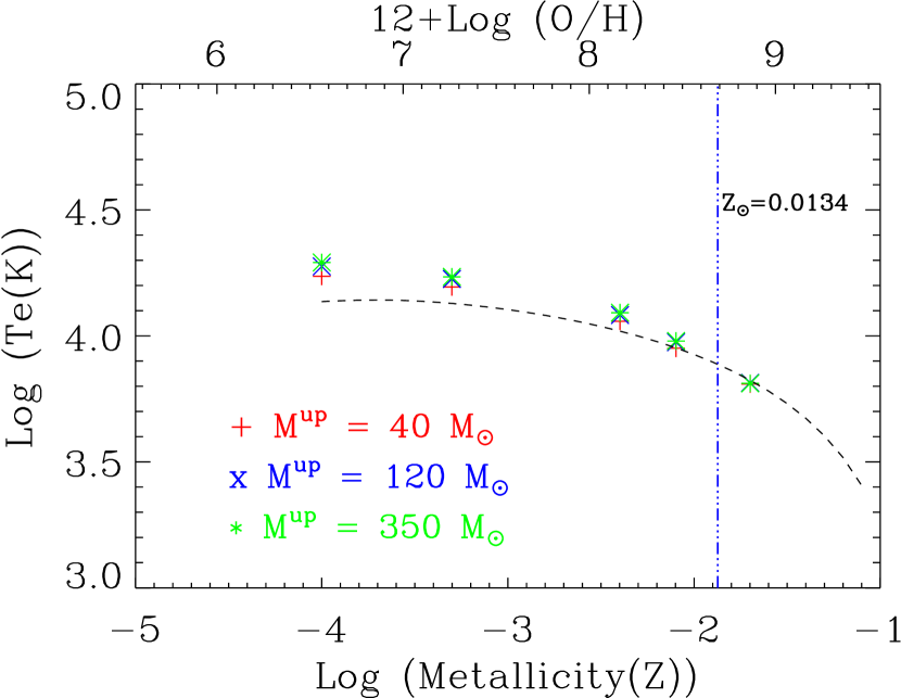
Figure 17: Plot of electron temperature T_e (obtained from CLOUDY) against metallicity Z for $M_{up}$ = 40, 120 and 350$~{}\rm{M}_{\sun}$ indicated by the red ’X’s, blue crosses and green xterisks respectively. The lower axis is the metallicity while the upper one is the corresponding oxygen abundance, $\rm{x}~{}=~{}12+\rm{log(O/H)}$. The blue dashed-dotted line indicates the metallicity at Z = 0.0134 which we adopted in this work as the solar metallicity. The average of the empirical fits derived by López-Sánchez et al. (2012) for high-ionization O iii and for low-ionization O ii zones is shown by the black dashed line.

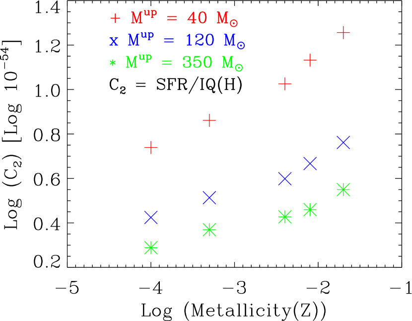
Figure 18: Variation of the constant ${C_{2}}$ with age at different metallicities (Z = 0.0001, 0.0005, 0.004, 0.008 and 0.02) and different upper mass limits. The symbols used to indicate the different $M_{up}$ are as in Figure 17. These variations of ${C_{2}}$, depending on the set of upper limits used, can severely underestimate or overestimate the estimated SFR using the thermal radio luminosity as a tracer. As clearly noticed, there is a large difference between $C_{2}$ obtained with $M_{up}=40~{}\rm{M}_{\sun}$ and $M_{up}=120~{}\rm{M}_{\sun}$ and that obtained with $M_{up}~{}=~{}120~{}\rm{M}_{\sun}$ and $M_{up}=350~{}\rm{M}_{\sun}$. $C_{2}$ is as defined in equation 8.

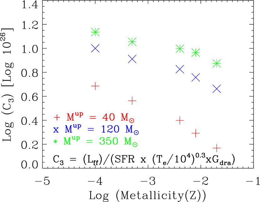
Figure 19: Same as in Figure 18 but for the constant $C_{3}$. $C_{3}$ is as defined in equation 11.

In Figure 17, we show the plot of electron temperature T_e (obtained from CLOUDY) against metallicity Z for $M_{up}$ = 40, 120 and 350. The oxygen abundance corresponding to the metallicity Z, written as $\rm{x}=12+\ log(\rm{O/H})$ where $\rm{O/H}~{}=~{}\rm{O/H}_{\sun}+\log(Z/Z_{\sun}$, is shown on the upper axis. To convert from Z to (O/H), we adopt the solar oxygen abundance given by Asplund et al. (2009), $\rm{x}_{\sun}=12+\log(\rm{O/H})_{\sun}=8.69\pm 0.05$ and $Z_{\sun}=0.0134$ and thus x  =  8.69 + log(Z/0.0134). The blue vertical dotted line indicates this solar metallicity value of 0.0134. The average of the empirical fits derived by López-Sánchez et al. (2012) for high-ionization O iii and for low-ionization O ii zones, using the MAPPINGS III code (Sutherland & Dopita, 1993), is shown as the dashed black lines. In this figure, our $T_{e}$ values (’X’s, crosses and xterisks) computed with CLOUDY for different metallicities are compared with the above-mentioned empirical fit obatined by López-Sánchez et al. (2012). It can be seen that our $T_{e}$ values start deviating from those of López-Sánchez et al. (2012) at low metallicities. A multiple regression fitting relation between $T_{e}$, $M_{up}$ and Z that can be easily included in analytical approximations, is provided by equation 34.

$$\rm{log}\left(\frac{\rm{T}_{e}(\rm{Z},\rm{M}_{up})}{10^{4}~{}K}\right)=-0.13-0.19\rm{log}(Z/0.02)+0.03\rm{log}(\rm{M}_{up}/120)$$ (34)

Table 2 lists the values of the constants $C_{2}$ and $C_{3}$ in equations 8 and 11, obtained with our constant SFR models for different SSPs parameters. These values are shown in Figure 18. The multiple regression fitting relation is given by Equation 35.

$$\rm{log}(C_{2})=0.16\rm{log}(Z/0.02)-0.61\rm{log}(M_{up}/120)-53.18$$ (35)

Table 2 also lists the values of the constants $C_{3}$ in equation 11. These values are shown in Figure 19. The corresponding multiple regression fitting relation is given by Equation 36.

$$\rm{log}(C_{3})=0.61\rm{log}(M_{up}/120)-0.16\rm{log}(Z/0.02)+26.61$$ (36)

Using the relation  35 in Equation 8 we obtain the integrated ionizing photon flux of a star-forming region of arbitrary constant metallicity and IMF upper mass limit

$$\rm{log}(IQ(H))=$$

$$-0.16\rm{log}(Z/0.02)+0.61\rm{log}(M_{up}/120)+53.18]+\rm{log}(SFR)$$ (37)

while, using the relation 36 in Equation 11 ($\rm{T}_{e}$ in this Equation is in $10^{4}~{}K$), we may get the corresponding SFR-thermal radio calibration:

$$\rm{log}(SFR/L(\nu)_{\rm{ff}})=0.60\rm{log}(M_{up}/120)-0.10\rm{log}(Z/0.02)$$

$$-\rm{log}(G_{dra})-26.57$$ (38)

where SFR and $\nu$ are in units of $\rm{M}_{\sun}\rm{yr}^{-1}$ and GHz respectively. Similarly for SFR vs. H$\alpha$ calibration we may write:

$$\rm{log}(SFR/H\alpha)=0.16\rm{log}(Z/0.02)-0.61\rm{log}(M_{up}/120)-41.32$$ (39)

and for SFR vs. H$\beta$ calibration:

$$\rm{log}(SFR/H\beta)=0.16\rm{log}(Z/0.02)-0.61\rm{log}(M_{up}/120)-40.87$$ (40)

Comparisons between SFR calibrations derived using Equations  38 , 39 and 40 above and those obtained directly from our model are given in Table 4 and discussed in Section 5.1. The former case is indicated by the superscript ^ssp in this table.

Appendix B Best-fits derived quantities for M100 and NGC 6946 Star-forming regions

Table 3: GRASIL Best-fit model luminosities.

ID	${FUV_{i}}$	${FUV_{t}}$	$H\beta_{i}$	$H\beta_{t}$	$H\alpha_{i}$	$H\alpha^{\rm{data}}$	$H\alpha_{t}$	$24$	$70$	$FIR$	$1.4$	$4.9$	$8.5$	$33$	$q_{1.4}$	$MC$	$CIR$	$FIR/BOL$
(1)	(2)	(3)	(4)	(5)	(6)	(7)	(8)	(9)	(10)	(11)	(12)	(13)	(14)	(15)	(16)	(17)	(18)	(19)
	$10^{41}$	$10^{41}$	$10^{39}$	$10^{39}$	$10^{39}$	$10^{39}$	$10^{39}$	$10^{41}$	$10^{41}$	$10^{42}$	$10^{26}$	$10^{26}$	$10^{26}$	$10^{26}$
$M_{up}~{}=~{}40~{}\rm{M}_{\sun}$
M100	653.10	319.0	102.15	33.70	298.61	123.0	105.0	130.0	616.0	167.0	793.0 (2)	285.0 (5)	186.0 (8)	71.6 (18)	2.38	19	81	0.39
NGC 6946_1	4.52	2.03	1.92	0.95	5.48	3.96	2.88	0.77	2.81	0.66	2.28 (24)	1.1 (44)	0.87 (54)	0.55 (75)	2.53	25	75	0.62
NGC 6946_2	10.65	6.73	5.01	3.47	14.28	12.10	10.30	1.34	4.50	1.02	4.11 (37)	2.3 (59)	1.89 (68)	1.33 (85)	2.46	35	65	0.44
NGC 6946_3	4.52	2.20	1.92	1.02	5.48	4.86	3.07	0.47	2.85	0.60	2.28 (24)	1.1 (44)	0.87 (54)	0.55 (75)	2.53	28	72	0.58
NGC 6946_5	2.71	1.54	1.15	0.76	3.29	2.90	2.28	0.20	1.28	0.30	1.37 (24)	0.7 (44)	0.52 (54)	0.33 (75)	2.42	12	88	0.50
NGC 6946_6	12.47	5.22	4.86	2.17	13.87	7.87	6.59	2.92	8.41	2.01	7.99 (16)	3.6 (32)	2.68 (42)	1.55 (65)	2.47	27	73	0.66
NGC 6946_7	13.93	5.79	6.47	2.87	18.40	7.81	8.67	2.96	9.42	2.26	5.36 (36)	3.0 (58)	2.45 (67)	1.71 (84)	2.69	37	63	0.66
NGC 6946_8	9.90	4.99	4.59	2.66	13.08	2.73	8.02	1.42	5.75	1.29	3.81 (36)	2.1 (58)	1.74 (67)	1.21 (84)	2.61	21	80	0.57
NGC 6946_9	10.80	4.86	4.61	2.29	13.10	5.08	6.92	2.07	6.58	1.58	5.47 (24)	2.7 (44)	2.09 (54)	1.33 (75)	2.52	24	76	0.62
$M_{up}~{}=~{}120~{}\rm{M}_{\sun}$
M100	729.94	379.0	260.66	131.0	759.97	123.0	406.0	120.0	687.0	175.0	734.0 (7)	291.0 (15)	204.0 (21)	98.4 (42)	2.45	18	82	0.42
NGC 6946_1	3.77	1.29	1.82	0.63	5.17	3.96	1.94	0.83	3.33	0.70	2.26 (24)	1.1 (44)	0.87 (54)	0.55 (76)	2.60	212	78	0.69
NGC 6946_2	6.76	3.29	4.53	2.07	12.95	12.10	6.23	1.29	4.29	0.95	4.23 (35)	2.3 (57)	1.91 (66)	1.33 (84)	2.44	42	58	0.60
NGC 6946_3	3.01	0.99	1.85	0.71	5.28	4.86	2.19	0.57	3.02	0.63	1.96 (30)	1.0 (52)	0.82 (61)	0.55 (81)	2.62	21	79	0.70
NGC 6946_5	1.74	0.68	1.02	0.38	2.92	2.90	1.16	0.27	1.25	0.30	1.48 (21)	0.7 (40)	0.54 (49)	0.33 (72)	2.38	29	71	0.70
NGC 6946_6	10.69	3.49	5.12	1.55	14.66	7.87	4.79	2.85	9.27	2.02	6.32 (24)	3.1 (44)	2.43 (54)	1.55 (76)	2.60	26	74	0.70
NGC 6946_7	9.24	2.80	5.73	1.87	16.24	7.81	5.79	2.57	8.99	2.01	6.06 (30)	3.2 (52)	2.55 (61)	1.71 (81)	2.61	24	76	0.72
NGC 6946_8	6.57	2.28	4.07	1.61	11.55	2.73	4.97	1.54	6.26	1.32	4.30 (30)	2.2 (52)	1.81 (61)	1.21 (81)	2.60	21	79	0.68
NGC 6946_9	9.15	3.03	4.51	1.43	12.82	5.08	4.43	2.41	8.06	1.75	5.00 (28)	2.5 (49)	2.02 (58)	1.33 (79)	2.64	26	74	0.69

Col.(1): ID. Col.(2-7): luminosities at FUV (0.16 $\micron$), $H\beta$ and $H\alpha$. ⁱ and ^t indicates intrinsic and attenuated transmitted luminosities respectively. Col.(8): observed attenuation uncorrected $H\alpha$ luminosity. Cols.(9 and 10): luminosities at 24 $\micron$ and 70 $\micron$. Col.(11): total (3-1000 $\micron$)IR luminosity. Cols.(12-15): radio luminosities at 1.4, 4.9, 8.5 and 33 GHz. Enclosed in parenthesis is the fraction in  per cent of the thermal radio component to the total radio emission. Col.(16): q-parameter as defined by equation 1. Cols.(17 and 18) are the MC and cirrus contribution (in per cent) to the total IR luminosity respectively. Col.(19): ratio of the total IR and the bolometric luminosities All UV, optical and infrared luminosities are in $\rm{erg}\;\rm{s}^{-1}$ while all radio luminosities are in $\rm{erg}\;\rm{s}^{-1}\;\rm{Hz}^{-1}$. The corresponding SFR calibrations at these luminosities are given in Table 4.

Table 4: GRASIL Best-fit derived SFRs and their calibrations at various bands.

$ID$	$<SFR>$	$C(FUV_{i})$	$C(H\beta_{i})$	$C(H\beta_{i})^{ssp}$	$C(H\alpha_{i})$	$C(H\alpha_{i})^{ssp}$	$C(24)$	$C(70)$	$C(FIR)$	$C(1.4)$	$C(4.9)$	$C(8.5)$	$C(33)$	$C(33)^{ssp}$	$t$
(1)	(2)	(3)	(4)	(5)	(6)	(7)	(8)	(9)	(10)	(11)	(12)	(13)	(14)	(15)	(16)
		$10^{-43}$	$10^{-42}$	$10^{-42}$	$10^{-42}$	$10^{-42}$	$10^{-43}$	$10^{-43}$	$10^{-44}$	$10^{-28}$	$10^{-28}$	$10^{-28}$	$10^{-28}$	$10^{-28}$
$\rm{M}_{up}~{}=~{}40~{}\rm{M}_{\sun}$
M100	5.58	0.85	54.67	45.22	18.70	16.04	4.30	0.91	3.35	0.70 (2)	1.96 (5)	3.00 (8)	7.79 (18)	25.71	12.0
NGC 6946_1	0.09	1.88	44.33	31.96	15.5	11.34	11.01	3.02	12.80	3.72 (24)	7.62 (44)	9.72 (54)	15.4 (76)	14.77	8.0
NGC 6946_2	0.20	1.85	39.31	31.95	13.8	11.33	14.70	4.38	19.30	4.79 (37)	8.64 (59)	10.40 (68)	14.9 (85)	14.75	9.0
NGC 6946_3	0.09	1.88	44.22	31.96	15.5	11.34	18.01	2.98	14.20	3.72 (24)	7.62 (44)	9.72 (54)	15.4 (76)	14.77	8.0
NGC 6946_5	0.05	1.88	44.28	31.96	15.5	11.34	25.63	3.98	17.00	3.72 (50)	7.62 (71)	9.72 (78)	15.3 (90)	14.77	8.0
NGC 6946_6	0.20	1.58	40.51	31.99	14.2	11.35	6.75	2.34	9.79	2.47 (24)	5.53 (44)	7.36 (54)	12.8 (76)	14.79	12.0
NGC 6946_7	0.29	2.06	44.38	31.95	15.6	11.34	9.70	3.05	12.70	5.36 (17)	9.70 (33)	11.70 (42)	16.8 (66)	14.76	7.0
NGC 6946_8	0.20	2.06	44.46	31.95	15.6	11.34	14.37	3.55	15.80	5.36 (37)	9.70 (59)	11.70 (68)	16.8 (85)	14.76	7.0
NGC 6946_9	0.20	1.88	44.06	31.96	15.5	11.34	9.81	3.09	12.90	3.72 (37)	7.62 (59)	9.72 (68)	15.4 (85)	14.77	8.0
$<NGC~{}6946>$	0.20	1.88	44.25	31.96	15.5	11.34	12.69	3.07	13.55	3.72 (30)	7.62 (52)	9.72 (61)	15.4 (80)	14.77	8.0
$\rm{M}_{up}~{}=~{}120~{}\rm{M}_{\sun}$
M100	4.80	0.66	18.43	15.92	6.32	5.65	4.00	0.70	2.74	0.65 (24)	1.65 (44)	2.36 (54)	4.88 (76)	8.90	12.0
NGC 6946_1	0.03	0.80	16.44	11.46	5.80	4.07	3.61	0.90	4.30	1.34 (9)	2.73 (19)	3.48 (26)	5.48 (48)	5.27	11.0
NGC 6946_2	0.07	1.02	15.22	11.27	5.33	4.00	5.35	1.61	7.25	1.63 (26)	2.98 (46)	3.62 (56)	5.20 (77)	5.13	11.0
NGC 6946_3	0.03	0.90	14.62	11.46	5.11	4.07	4.78	0.89	4.27	1.38 (37)	2.64 (59)	3.27 (68)	4.88 (85)	5.26	8.0
NGC 6946_5	0.02	0.92	15.75	11.32	5.48	4.02	5.84	1.28	5.23	1.07 (32)	2.28 (53)	2.95 (63)	4.79 (82)	5.16	18.0
NGC 6946_6	0.09	0.80	16.59	11.46	5.80	4.07	2.98	0.92	4.19	1.34 (37)	2.73 (59)	3.48 (68)	5.48 (85)	5.27	11.0
NGC 6946_7	0.08	0.90	14.48	11.46	5.11	4.07	3.23	0.92	4.15	1.38 (23)	2.64 (42)	3.27 (52)	4.88 (74)	5.26	8.0
NGC 6946_8	0.06	0.90	14.51	11.46	5.11	4.07	3.83	0.94	4.48	1.38 (26)	2.64 (46)	3.27 (56)	4.88 (77)	5.26	8.0
NGC 6946_9	0.07	0.82	16.63	11.46	5.85	4.07	3.11	0.93	4.29	1.51 (32)	2.97 (53)	3.72 (63)	5.68 (82)	5.26	9.0
$<NGC~{}6946>$	0.06	0.90	15.49	11.46	5.41	4.07	3.72	0.93	4.29	1.38 (29)	2.69 (50)	3.38 (60)	5.04 (80)	5.26	10.0
Literature
		0.44a	75.8h		7.94b		2.46d	0.97g	4.55b	0.64a	1.4e	2.0e	6.53a
					5.30c		4.80h	0.92h	3.88a	0.62e
					6.62h			0.58f	3.99h

Col.(1): ID. Col.(2): average SFR (in $M_{\sun}\;yr^{-1}$) derived by considering the last 100 Myr time interval for the normal star-forming galaxy M100 and the age of the burst in the star-forming regions of NGC 6946 Cols.(3-15): SFR calibrations obtained using the above averaged SFR and the luminosities (intrinsic values for FUV, H$\alpha$ and H$\beta$ ) given in Table 3. In Cols.5, 7 and 15, we rather present the calibrations obtained from simple SSPs models, Equations 40 , 39 and 38 respectively for H$\beta$, H$\alpha$ and 33GHz. The later refers to free-free emission. For the radio -based SFR calibration, we enclosed in parenthesis the percentage contribution of the thermal radio component to the total radio emission. Col.(16): age of the galaxy in Gyr for M100 or the age of the burst in Myr, for NGC 6946 extranuclear regions. The last row in the first and second panels (with ID, $<NGC~{}6946>$) gives the median values of all quantities given for NGC 6946 star-bursting regions. The values of the SFR calibrations given in the 3rd panel were taken from the literature. The superscript on these values indicates the reference as described below: ^aMurphy et al. (2011), ^bKennicutt (1998), ^cCalzetti et al. (2007), ^dZhu et al. (2008), ^eSchmitt et al. (2006), ^fLi et al. (2010), ^gLawton et al. (2010), ^hPanuzzo et al. (2003). These authors adopted different IMF and evolutionary synthesis models.

Table 5: GRASIL Best-fit derived quantities related to dust attenuation.

ID	$A_{H\alpha}$	$A_{H\beta}$	$A_{FUV}$	$A_{NUV}$	$A_{B}$	$A_{48}$	$A_{V}$	$A_{65}$	$\tau_{1}$	$R_{V}$	$E(H\beta-H\alpha)^{c}$	$E(H\beta-H\alpha)^{l}$	$t_{esc}$
(1)	(2)	(3)	(4)	(5)	(6)	(7)	(8)	(9)	(10)	(11)	(12)	(13)	(14)
	$M_{up}~{}=~{}40~{}\rm{M}_{\sun}$
M100	1.13	1.20	0.78	0.83	0.30	0.28	0.24	0.23	17.79	4.17	0.055	0.093	2.5
NGC 6946_1	0.70	0.76	0.87	0.91	0.60	0.63	0.54	0.57	12.66	8.08	0.060	0.059	1.0
NGC 6946_2	0.36	0.40	0.50	0.53	0.31	0.33	0.27	0.29	15.38	6.03	0.041	0.037	0.5
NGC 6946_3	0.63	0.69	0.78	0.82	0.53	0.56	0.47	0.51	26.84	7.34	0.056	0.055	1.0
NGC 6946_5	0.40	0.45	0.61	0.65	0.43	0.42	0.39	0.37	8.43	9.14	0.053	0.054	0.3
NGC 6946_6	0.81	0.88	0.95	0.99	0.67	0.71	0.60	0.66	8.51	8.62	0.056	0.067	1.2
NGC 6946_7	0.82	0.88	0.96	0.99	0.67	0.73	0.59	0.66	17.67	7.71	0.062	0.059	1.0
NGC 6946_8	0.53	0.59	0.75	0.79	0.53	0.54	0.48	0.48	9.63	9.48	0.059	0.053	0.6
NGC 6946_9	0.70	0.76	0.87	0.91	0.60	0.63	0.54	0.57	8.79	8.08	0.060	0.060	1.0
	$M_{up}~{}=~{}120~{}\rm{M}_{\sun}$
M100	0.68	0.75	0.71	0.77	0.30	0.30	0.24	0.23	20.16	4.18	0.070	0.087	0.9
NGC 6946_1	1.07	1.16	1.18	1.24	0.82	0.95	0.75	0.78	9.28	9.48	0.173	0.088	0.6
NGC 6946_2	0.79	0.85	0.78	0.84	0.53	0.77	0.45	0.58	19.10	5.28	0.188	0.055	1.0
NGC 6946_3	0.96	1.04	1.20	1.26	0.86	0.93	0.78	0.79	16.11	10.38	0.136	0.087	0.9
NGC 6946_5	0.99	1.06	1.01	1.08	0.73	0.96	0.65	0.77	21.31	7.51	0.190	0.062	1.0
NGC 6946_6	1.21	1.30	1.21	1.28	0.84	1.01	0.75	0.81	9.05	8.92	0.201	0.084	0.7
NGC 6946_7	1.13	1.22	1.30	1.36	0.91	1.02	0.82	0.87	9.08	9.71	0.152	0.086	1.0
NGC 6946_8	0.92	1.01	1.15	1.21	0.82	0.89	0.74	0.76	9.26	10.03	0.135	0.085	0.9
NGC 6946_9	1.16	1.25	1.20	1.27	0.83	1.00	0.75	0.80	9.11	9.10	0.194	0.087	0.6

Col.(1) :ID. Cols.(2 - 9) give the attenuations in H$\alpha$, H$\beta$, FUV (0.16$\micron$), NUV (0.20 $\micron$), B-band(0.45 $\micron$), the interpolated continum at H$\beta$, V-band(0.55 $\micron$) and the interpolated continum at H$\alpha$. They were derived using the ratio of the intrinsic unattenuated and attenuated (observed) fluxes. Col.(10): optical depth of the molecular cloud at 1 $\micron$. Col.(11): $R_{V}$. Col.(12):The reddening given simply by A₄₈ - A₆₅. Col.(13):The reddening derived using the balmer decrement method as given by Equation 28. Col.(14): escape time of young stars from their birth cloud in Myr.

References

- Allard et al. (1997) Allard F., Hauschildt P. H., Alexander D. R., Starrfield S., 1997, ARA&A, 35, 137
- Asplund et al. (2009) Asplund M., Grevesse N., Sauval A. J., Scott P., 2009, ARA&A, 47, 481
- Berkhuijsen (1984) Berkhuijsen E. M., 1984, A&A, 140, 431
- Bicker & Fritze-v. Alvensleben (2005) Bicker J., Fritze-v. Alvensleben U., 2005, A&A, 443, L19
- Bressan et al. (2013) Bressan A., Marigo P., Girardi L., Nanni A., Rubele S., 2013, in European Physical Journal Web of Conferences, Vol. 43, European Physical Journal Web of Conferences, p. 3001
- Bressan et al. (2012) Bressan A., Marigo P., Girardi L., Salasnich B., Dal Cero C., Rubele S., Nanni A., 2012, MNRAS, 427, 127
- Bressan, Silva & Granato (2002) Bressan A., Silva L., Granato G. L., 2002, A&A, 392, 377
- Calzetti et al. (2000) Calzetti D., Armus L., Bohlin R. C., Kinney A. L., Koornneef J., Storchi-Bergmann T., 2000, ApJ, 533, 682
- Calzetti et al. (2007) Calzetti D. et al., 2007, ApJ, 666, 870
- Cardelli, Clayton & Mathis (1989) Cardelli J. A., Clayton G. C., Mathis J. S., 1989, ApJ, 345, 245
- Castelli & Kurucz (2004) Castelli F., Kurucz R. L., 2004, ArXiv Astrophysics e-prints
- Charlot & Bruzual (1991) Charlot S., Bruzual A. G., 1991, ApJ, 367, 126
- Charlot & Fall (2000) Charlot S., Fall S. M., 2000, ApJ, 539, 718
- Chen et al. (2015) Chen Y., Bressan A., Girardi L., Marigo P., Kong X., Lanza A., 2015, MNRAS, 452, 1068
- Chen et al. (2014) Chen Y., Girardi L., Bressan A., Marigo P., Barbieri M., Kong X., 2014, MNRAS, 444, 2525
- Chiosi, Bertelli & Bressan (1988) Chiosi C., Bertelli G., Bressan A., 1988, A&A, 196, 84
- Condon (1992) Condon J. J., 1992, ARA&A, 30, 575
- Condon & Yin (1990) Condon J. J., Yin Q. F., 1990, ApJ, 357, 97
- Draine (2011) Draine B. T., 2011, Physics of the Interstellar and Intergalactic Medium
- Ertl et al. (2015) Ertl T., Janka H.-T., Woosley S. E., Sukhbold T., Ugliano M., 2015, ArXiv e-prints
- Fan et al. (2014) Fan L.-L., Lapi A., Bressan A., Nonino M., De Zotti G., Danese L., 2014, Research in Astronomy and Astrophysics, 14, 15
- Ferland (1996) Ferland G., 1996, Hazy: A Brief Introduction to CLOUDY. Univ. of Kentucky Physics Department Internal Report
- Girardi et al. (2002) Girardi L., Bertelli G., Bressan A., Chiosi C., Groenewegen M. A. T., Marigo P., Salasnich B., Weiss A., 2002, A&A, 391, 195
- Granato et al. (2000) Granato G. L., Lacey C. G., Silva L., Bressan A., Baugh C. M., Cole S., Frenk C. S., 2000, ApJ, 542, 710
- Heckman et al. (1983) Heckman T. M., van Breugel W., Miley G. K., Butcher H. R., 1983, AJ, 88, 1077
- Helou et al. (1988) Helou G., Khan I. R., Malek L., Boehmer L., 1988, ApJS, 68, 151
- Helou, Soifer & Rowan-Robinson (1985) Helou G., Soifer B. T., Rowan-Robinson M., 1985, ApJ, 298, L7
- Hummer & Storey (1987) Hummer D. G., Storey P. J., 1987, MNRAS, 224, 801
- Israel & Kennicutt (1980) Israel F. P., Kennicutt R. C., 1980, Astrophys. Lett., 21, 1
- Janka (2012) Janka H.-T., 2012, Annual Review of Nuclear and Particle Science, 62, 407
- Kennicutt (1983) Kennicutt, Jr. R. C., 1983, ApJ, 272, 54
- Kennicutt (1998) Kennicutt, Jr. R. C., 1998, ARA&A, 36, 189
- Kennicutt et al. (2003) Kennicutt, Jr. R. C. et al., 2003, PASP, 115, 928
- Kennicutt et al. (2009) Kennicutt, Jr. R. C. et al., 2009, ApJ, 703, 1672
- Kroupa (2001) Kroupa P., 2001, MNRAS, 322, 231
- Kurucz (1993) Kurucz R. L., 1993, in Astronomical Society of the Pacific Conference Series, Vol. 44, IAU Colloq. 138: Peculiar versus Normal Phenomena in A-type and Related Stars, Dworetsky M. M., Castelli F., Faraggiana R., eds., p. 87
- Lawton et al. (2010) Lawton B. et al., 2010, ApJ, 716, 453
- Li et al. (2010) Li Y., Calzetti D., Kennicutt R. C., Hong S., Engelbracht C. W., Dale D. A., Moustakas J., 2010, ApJ, 725, 677
- López-Sánchez et al. (2012) López-Sánchez Á. R., Dopita M. A., Kewley L. J., Zahid H. J., Nicholls D. C., Scharwächter J., 2012, MNRAS, 426, 2630
- Maeder & Meynet (1988) Maeder A., Meynet G., 1988, A&AS, 76, 411
- Maraston (2005) Maraston C., 2005, MNRAS, 362, 799
- Marigo & Girardi (2007) Marigo P., Girardi L., 2007, A&A, 469, 239
- Marigo et al. (2017) Marigo P. et al., 2017, ApJ, 835, 77
- Murphy et al. (2012) Murphy E. J. et al., 2012, ApJ, 761, 97
- Murphy et al. (2011) Murphy E. J. et al., 2011, ApJ, 737, 67
- Murphy et al. (2010) Murphy E. J. et al., 2010, ApJ, 709, L108
- O’Connor & Ott (2011) O’Connor E., Ott C. D., 2011, ApJ, 730, 70
- Oster (1961) Oster L., 1961, Reviews of Modern Physics, 33, 525
- Osterbrock (1989) Osterbrock D. E., 1989, Astrophysics of gaseous nebulae and active galactic nuclei. University Science Books, Mill Valley, CA
- Panuzzo et al. (2003) Panuzzo P., Bressan A., Granato G. L., Silva L., Danese L., 2003, A&A, 409, 99
- Pauldrach, Puls & Kudritzki (1986) Pauldrach A., Puls J., Kudritzki R. P., 1986, A&A, 164, 86
- Rubin (1968) Rubin R. H., 1968, ApJ, 154, 391
- Sander et al. (2015) Sander A., Shenar T., Hainich R., Gímenez-García A., Todt H., Hamann W.-R., 2015, A&A, 577, A13
- Schmitt et al. (2006) Schmitt H. R., Calzetti D., Armus L., Giavalisco M., Heckman T. M., Kennicutt, Jr. R. C., Leitherer C., Meurer G. R., 2006, ApJ, 643, 173
- Silva et al. (1998) Silva L., Granato G. L., Bressan A., Danese L., 1998, ApJ, 509, 103
- Silva et al. (2011) Silva L. et al., 2011, MNRAS, 410, 2043
- Spera, Mapelli & Bressan (2015) Spera M., Mapelli M., Bressan A., 2015, MNRAS, 451, 4086
- Sukhbold & Woosley (2014) Sukhbold T., Woosley S. E., 2014, ApJ, 783, 10
- Sutherland & Dopita (1993) Sutherland R. S., Dopita M. A., 1993, ApJS, 88, 253
- Tang et al. (2014) Tang J., Bressan A., Rosenfield P., Slemer A., Marigo P., Girardi L., Bianchi L., 2014, MNRAS, 445, 4287
- Ugliano et al. (2012) Ugliano M., Janka H.-T., Marek A., Arcones A., 2012, ApJ, 757, 69
- Vega et al. (2008) Vega O., Clemens M. S., Bressan A., Granato G. L., Silva L., Panuzzo P., 2008, A&A, 484, 631
- Vega et al. (2005) Vega O., Silva L., Panuzzo P., Bressan A., Granato G. L., Chavez M., 2005, MNRAS, 364, 1286
- Wofford et al. (2016) Wofford A. et al., 2016, MNRAS, 457, 4296
- Young et al. (1989) Young J. S., Xie S., Kenney J. D. P., Rice W. L., 1989, ApJS, 70, 699
- Zhu et al. (2008) Zhu Y.-N., Wu H., Cao C., Li H.-N., 2008, ApJ, 686, 155