The Gravitational Wave Background from Massive Black Hole Binaries in Illustris: spectral features and time to detection with pulsar timing arrays

Abstract

Pulsar Timing Arrays (PTA) around the world are using the incredible consistency of millisecond pulsars to measure low frequency gravitational waves from (super)Massive Black Hole (MBH) binaries. We use comprehensive MBH merger models based on cosmological hydrodynamic simulations to predict the spectrum of the stochastic Gravitational-Wave Background (GWB). We use real Time-of-Arrival (TOA) specifications from the European, NANOGrav, Parkes, and International PTA (IPTA) to calculate realistic times to detection of the GWB across a wide range of model parameters. In addition to exploring the parameter space of environmental hardening processes (in particular: stellar scattering efficiencies), we have expanded our models to include eccentric binary evolution which can have a strong effect on the GWB spectrum. Our models show that strong stellar scattering and high characteristic eccentricities enhance the GWB strain amplitude near the PTA sensitive “sweet-spot” (near the frequency $f=1\,\textrm{yr}^{-1}$), slightly improving detection prospects in these cases. While the GWB amplitude is degenerate between cosmological and environmental parameters, the location of a spectral turnover at low frequencies ($f\lesssim 0.1\,\textrm{yr}^{-1}$) is strongly indicative of environmental coupling. At high frequencies ($f\gtrsim 1\,\textrm{yr}^{-1}$), the GWB spectral index can be used to infer the number density of sources and possibly their eccentricity distribution. Even with merger models that use pessimistic environmental and eccentricity parameters, if the current rate of PTA expansion continues, we find that the International PTA is highly likely to make a detection within about 10 years.

1 Introduction

Pulsar Timing Arrays (PTA) are expected to detect Gravitational Waves (GW; Sazhin, 1978; Detweiler, 1979; Romani & Taylor, 1983) from stable binaries of (super)-Massive Black Holes (MBH; Rajagopal & Romani, 1995; Wyithe & Loeb, 2003; Phinney, 2001). These arrays use correlated signals in the consistently timed pulses from millisecond pulsars to search for low-frequency ($\lesssim 10\,\textrm{yr}^{-1}$) perturbations to flat space-time (Hellings & Downs, 1983; Foster & Backer, 1990). There are currently three independent PTA searching for GW signals: the North-American Nanohertz Observatory for Gravitational waves (NANOGrav; McLaughlin, 2013), the European PTA (EPTA; Kramer & Champion, 2013), and the Parkes PTA (PPTA; Manchester et al., 2013). Additionally, the International PTA (IPTA, Hobbs et al., 2010) is a collaboration which aims to combine the data and expertise from each independent group.

Comparable upper limits on the presence of a stochastic Gravitational Wave Background (GWB) have been calculated by the EPTA (Lentati et al., 2015), NANOGrav (Arzoumanian et al., 2015), PPTA (Shannon et al., 2015) and IPTA (Verbiest et al., 2016). These upper limits are already astrophysically informative in that much of the previously predicted parameter space is now in tension with observations, and there are suggestions that some models are excluded (Shannon et al., 2015). Many previous GWB models have assumed that most or all of the MBH pairs formed after the merger of their host galaxies are able to quickly reach the ‘hard binary’ phase ($\lesssim 10\,\mathrm{pc}$) and eventually coalesce due to GW emission (e.g. Wyithe & Loeb, 2003; Jaffe & Backer, 2003; Sesana, 2013). These models, which assume GW-only driven evolution and produce purely power-law GWB spectra, likely over-predict the GWB energy in that: 1) perhaps a substantial fraction of MBH Binaries stall at galactic scales ($\sim$ kpc), or before reaching the small separations (${\sim}10^{-3}$–$10^{-1}\,\mathrm{pc}$) corresponding to the PTA sensitive band (e.g. McWilliams et al., 2014); and 2) significant ‘attenuation’ of the GW signal may exist due to environmental processes (non-GW hardening, due to stellar scattering or coupling with a circumbinary gaseous disk) which decrease the amount of time binaries spend in a given frequency interval (e.g. Kocsis & Sesana, 2011; Sesana, 2013; Ravi et al., 2014; Rasskazov & Merritt, 2016).

Some recent GW-only models predict lower signal levels because of differing cosmological assumptions (i.e. galaxy-galaxy merger rates, the mass functions of MBH, etc) which produce different distributions of MBH binaries (e.g. Roebber et al., 2016; Sesana et al., 2016), eliminating the tension with PTA upper limits. More comprehensive models have also been assembled which take into account binary-stalling and GW-attenuation (e.g. Ravi et al., 2014). Some of these models suggest that the GWB is only just below current observational sensitivities, which begs the question, ‘how long until we make a detection?’ Recently, PTA detection statistics conveniently formalized in Rosado et al. (2015) have been used by Taylor et al. (2016) to calculate times to detections for purely power-law, GW-only GWB models with a full range of plausible GWB amplitudes. Vigeland & Siemens (2016) also calculate detection statistics using a more extensive suite of broken power-laws to model the effects of varying environmental influences.

In Kelley et al. (2016, hereafter ‘KBH-16’) we construct the most comprehensive MBHB merger models to date, using the self-consistently derived population of galaxies and MBH from the Illustris cosmological, hydrodynamic simulations (§2.1, e.g. Vogelsberger et al., 2014b; Genel et al., 2014). The MBHB population is post-processed using semi-analytic models of GW emission in addition to environmental hardening mechanisms that are generally required for MBHB to reach small separations within a Hubble time (e.g. Begelman et al., 1980; Milosavljević & Merritt, 2003), and emit GW in PTA-sensitive frequency bands.

In this paper, we introduce the addition of eccentric binary evolution to our models, and explore its effects on the GWB. To produce more realistic GWB spectra, we complement our previous semi-analytic (SA) calculations with a more realistic, Monte-Carlo (MC) technique. Using our merger models and resulting spectra, we calculate realistic times to detection for each PTA following Rosado et al. (2015) & Taylor et al. (2016). In §2 we describe our MBHB, GWB and PTA models. Then in §3 we describe the effects of eccentricity on binary evolution (§3.1) and the GWB spectrum (§3.2) including comparisons between the SA and MC calculations, and finally our predictions for times to GWB detections (§3.3).

2 Methods

Our simulations use the coevolved galaxies and MBH particles from the Illustris cosmological, hydrodynamic simulations (Vogelsberger et al., 2013; Torrey et al., 2014; Vogelsberger et al., 2014a; Genel et al., 2014; Sijacki et al., 2015) run using the Arepo ‘moving-mesh’ code (Springel, 2010). Our general procedure of extracting MBH, their merger events and their galactic environments are described in detail in KBH-16. Here, we give a brief overview of our methods (§2.1) and the improvements made to include eccentric binary evolution (§2.2). We then describe the methods by which we calculate GW signatures (§2.3) and realistic detection statistics for simulated PTA (§2.4).

2.1 Illustris MBH Mergers and Environments

The Illustris simulation is a cosmological box of $106.5\,\mathrm{Mpc}$ on a side (at $z=0.0$) containing moving-mesh gas cells, and particles representing stars, dark matter, and MBH. All of the Illustris data is publicly available online (Nelson et al., 2015). MBH are ‘seeded’ with a mass of $1.42\times\nobreak 10^{5}\,\textrm{M}_{\odot}$ into halos with masses above $7.1\times\nobreak 10^{10}\,\textrm{M}_{\odot}$ (Sijacki et al., 2015), where they accrete gas from the local environment and grow over time. As they develop, they proportionally deposit energy back into the local environment (Vogelsberger et al., 2013). When two MBH particles come within a gravitational smoothing length of one another (typically on the order of a $\mathrm{kpc}$) a ‘merger’ event is recorded. From those mergers we identify the constituent MBH and the host galaxy in which they subsequently reside. From the host galaxy, density profiles are constructed which are used to determine the environment’s influence on the MBHB merger process. The simulations used here, as in KBH-16, are semi-analytic models which integrate each binary (independently) from large-scale separations down to eventual coalescence based on prescriptions for GW- and environmentally- driven hardening.

2.2 Models for Eccentric Binary Evolution

We implement four distinct mechanisms which dissipate orbital energy and ‘harden’ the MBHB (as in KBH-16):

• Dynamical Friction (DF, dominant on ${\sim}\mathrm{kpc}$ scales) is implemented following Chandrasekhar (1943) and Binney & Tremaine (1987), based on the local density (gas and dark matter) and velocity dispersion. The mass of the decelerating object is taken as the mass of the secondary MBH along with its host galaxy. We assume a model for tidal stripping such that the decelerating mass decreases as a power-law from the combined mass, to that of only the secondary MBH, over the course of a dynamical time. With the addition of eccentric binary evolution, we make the approximation that DF does not noticeably affect the eccentricity distribution of binaries (e.g. Colpi et al., 1999; van den Bosch et al., 1999; Hashimoto et al., 2003), and that the semi-major axis remains the relevant distance scale. Equivalently, the “initial” eccentricities in our models can be viewed as the eccentricity once binaries enter the stellar scattering regime.

• Stellar Loss-Cone (LC) scattering (${\sim}\mathrm{pc}$), is implemented using the prescription from Sesana et al. (2006) & Sesana (2010) following the formalism of Quinlan (1996). Here, the hardening rate ($da/dt$) and eccentricity evolution ($de/dt$) are determined by dimensionless constants $H$ and $K$, calculated in numerical scattering experiments such that,

  $$\frac{da}{dt}\bigg{|}_{u}\equiv-\frac{G\rho}{\sigma}a^{2}\,H,$$ (1)

  and

  $$\frac{de}{dt}\bigg{|}_{u}\equiv\frac{G\rho}{\sigma}a\,H\,K.$$ (2)

  Here the binary separation (semi-major axis, $a$) and eccentricity ($e$) are evolved based on profiles of density ($\rho$) and velocity dispersion ($\sigma$) calculated from each binary host-galaxy in Illustris. We use the fitting formulae and tabulated constants for $H$ and $K$ from Sesana et al. (2006). Note that this semi-empirical approach, which we will refer to as ‘eccentric LC models’, explicitly assumes a full loss-cone in the scattering experiments by which they are calibrated.

  In our previous calculations presented in KBH-16, we used a different LC prescription for binaries restricted to circular orbits. In this paper we focus on the eccentric LC models, but include results with our previous ‘circular’ prescription for comparison. The circular models include a dimensionless ‘refilling parameter’, ${\mathcal{F}_{\textrm{\tiny{refill}}}\in\{0.0,1.0\}}$, which interpolates between a ‘steady-state’ LC (${\mathcal{F}_{\textrm{\tiny{refill}}}=0.0}$), where equilibrium is reached between the scattering rate and refilling by the two-body diffusion of stars; and a ‘full’ LC ($\mathcal{F}_{\textrm{\tiny{refill}}}=1.0$), where the stellar distribution function is unaltered by the presence of the scattering source. The $\mathcal{F}_{\textrm{\tiny{refill}}}$ parameter for true astrophysical binaries is highly uncertain, but can drastically affect the efficiency with which binaries coalesce (see the discussion in KBH-16, ). We explore six models with, ${\mathcal{F}_{\textrm{\tiny{refill}}}=[0.0,\,0.2,\,0.4,\,0.6,\,0.8,\,1.0]}$. Some recent studies tend to favor nearly-full LC models (e.g. Sesana & Khan, 2015; Vasiliev et al., 2015). The eccentric LC model, with imposed zero-eccentricities ($e_{0}=0.0$), yields results very similar to the circular-only model with a full LC ($\mathcal{F}_{\textrm{\tiny{refill}}}=1.0$), as expected.

• Gas drag from a circumbinary, Viscous Disk (VD; ${\sim}10^{-3}\,\mathrm{pc}$) is calculated following the thin disk models from Haiman et al. (2009). In these models, the disk is composed of three, physically distinct regions (Shapiro & Teukolsky, 1986) determined by the dominant pressure (radiation versus thermal) and opacity (Thomson versus free-free) sources. From inner- to outer- disk, the regions are: 1) radiation & Thomson, 2) thermal & Thomson, and 3) thermal & free-free. The disk density profiles are constructed based on the self-consistently derived accretion rates given by Illustris, and truncated based on a (Toomre) gravitational stability criterion. Higher densities resulting from higher accretion rates lead to more extended inner-disk regions. We use an alpha-disk throughout. It’s worth noting that the inner-disk region (1) has a very similar hardening curve to GW-emission: ${\scalebox{1.2}{$\uptau$}_{\textrm{VD,1}}\propto r^{7/2}}$, versus ${\scalebox{1.2}{$\uptau$}_{\textrm{gw}}\propto r^{4}}$. In Illustris, post-merger MBH tend to have higher accretion rates, and thus larger inner-disk regions.

  We assume that the disk has a negligible effect on the eccentric evolution of binaries, i.e. ${\left[de/dt\right]_{\textrm{VD}}=0}$. This assumption is made for simplicity. While numerous studies have shown that eccentric evolution can at times be significant in circumbinary disks (e.g. Armitage & Natarajan, 2005; Cuadra et al., 2009; Roedig et al., 2011), we are unaware of generalized descriptions of eccentricity evolution for binaries/disks with arbitrary initial configurations. In the analysis which follows, we explore a wide range of eccentricity parameter space. While a given model may end up being inconsistent with VD eccentric-evolution, the overall parameter space should still encompass the same resulting GWB spectra.

• Gravitational Wave (GW) emission (${\sim}10^{-5}\,\mathrm{pc}$) hardens binaries at a rate given by Peters (1964, Eq. 5.6) as,

  $$\frac{da}{dt}=-\frac{64\,G^{3}}{5\,c^{5}}\frac{M_{1}\,M_{2}\left(M_{1}+M_{2}\right)}{a^{3}}\,F(e),$$ (3)

  where the eccentric enhancement,

  $$F(e)\equiv\frac{\left(1+\frac{73}{24}e^{2}+\frac{37}{96}e^{4}\right)}{\left(1-e^{2}\right)^{7/2}}.$$ (4)

  In KBH-16 we made the approximation that the eccentricity of all binaries was negligible and thus ${F(e)=1}$. Here, we include models with non-zero eccentricity, evolved as (Peters, 1964, Eq. 5.7),

  $$\frac{de}{dt}=-\frac{304\,G^{3}}{15\,c^{5}}\frac{M_{1}\,M_{2}\left(M_{1}+M_{2}\right)}{a^{4}}\frac{\left(e+\frac{121}{304}e^{3}\right)}{\left(1-e^{2}\right)^{5/2}}.$$ (5)

2.3 Gravitational Waves from Eccentric MBH Binaries

Circular binaries, with (rest-frame) orbital frequencies $f_{\textrm{\tiny{r}}}$, emit GW monochromatically at $2f_{\textrm{\tiny{r}}}$, i.e. the $n=2$ harmonic. Eccentric systems lose symmetry, and emit at $n=1$ and all higher harmonics, i.e. $f_{\textrm{\tiny{h}}}=n\,f_{\textrm{\tiny{r}}}$ (for $n\in\mathbb{I}$). The GW energy spectrum can then be expressed as (Enoki & Nagashima, 2007, Eq. 3.10),

$$\frac{d\varepsilon_{\textrm{\tiny{GW}}}}{df_{\textrm{\tiny{r}}}}=\sum_{n=1}^{\infty}\left[L_{\textrm{GW,circ}}(f_{\textrm{\tiny{h}}})\frac{\scalebox{1.2}{$\uptau$}_{\textrm{h}}^{f}(f_{\textrm{\tiny{h}}},e)}{n\,f_{\textrm{\tiny{h}}}}\,g(n,e)\right]_{f_{\textrm{\tiny{h}}}=f_{\textrm{\tiny{r}}}/n}.$$ (6)

The GW frequency-distribution function $g(n,e)$ is shown in Eq. 19. Equation (6) describes the GW spectrum emitted by a binary over its lifetime, which is used in the semi-analytic GWB calculation (§2.3.1). The total power radiated by an eccentric binary is enhanced by the factor $F(e)$, i.e., $L_{\textrm{GW}}(f_{\textrm{\tiny{r}}},e)=L_{\textrm{GW,circ}}(f_{\textrm{\tiny{r}}})\cdot F(e)$, where the GW luminosity for a circular binary is (Peters & Mathews, 1963, Eq. 16),

$$L_{\textrm{GW,circ}}(f_{\textrm{\tiny{r}}})=\frac{32}{5Gc^{5}}\left(G\mathcal{M}\,2\pi f_{\textrm{\tiny{r}}}\right)^{10/3}.$$ (7)

Note that in Eq. 6, the relevant timescale is the hardening-time (or ‘residence’-time) in frequency,

$$\scalebox{1.2}{$\uptau$}_{\textrm{h}}^{f}\equiv\left|\frac{f}{df/dt}\right|=\frac{2}{3}\left|\frac{a}{da/dt}\right|\equiv\frac{2}{3}\scalebox{1.2}{$\uptau$}_{\textrm{h}},$$ (8)

which is $2/3$ the hardening-time in separation (via Kepler’s law), which we use for most of our discussion and figures.

The GW strain from an individual, eccentric source can be related to that of a circular source as (e.g. Amaro-Seoane et al., 2010, Eq. 9),

$$h_{\textrm{\tiny{s}}}^{2}(f_{\textrm{\tiny{r}}})=\sum_{n=1}^{\infty}h_{\textrm{\tiny{s,circ}}}^{2}(f_{\textrm{\tiny{h}}})\left(\frac{2}{n}\right)^{2}\,g(n,e)\bigg{|}_{f_{\textrm{\tiny{h}}}=f_{\textrm{\tiny{r}}}/n}.$$ (9)

Here, the GW strain from a circular binary is,

$$h_{\textrm{\tiny{s,circ}}}(f_{\textrm{\tiny{r}}})=\frac{8}{10^{1/2}}\frac{\left(G\mathcal{M}\right)^{5/3}}{c^{4}\,d_{\textrm{\tiny{L}}}}\left(2\pi f_{\textrm{\tiny{r}}}\right)^{2/3}$$ (10)

(e.g. Sesana et al., 2008, Eq. 8), for a luminosity distance $d_{\textrm{\tiny{L}}}$, and a chirp mass $\mathcal{M}=\left(M_{1}M_{2}\right)^{3/5}/\left(M_{1}+M_{2}\right)^{1/5}$. Equation (9) describes the instantaneous GW strain amplitude from a binary, and is used in the Monte-Carlo GWB calculation (§2.3.2).

The GWB is usually calculated in one of two ways (Sesana et al., 2008): either Semi-Analytically (SA), treating the distribution of binaries as a smooth, continuous and deterministic function to calculate $\partial^{5}n_{c}(M_{1},M_{2},z,f_{r},e)/\partial M_{1}\partial M_{2}\partial z\partial f_{r}\partial e$ (Phinney, 2001), or alternatively, in the Monte Carlo (MC) approach, where $n_{c}(M_{1},M_{2},z,f_{r},e)$ is considered as a particular realization of a finite number of MBHB in the universe (Rajagopal & Romani, 1994).

2.3.1 Semi Analytic GWB

The GWB spectrum can be calculated from a distribution of eccentric binaries as (Huerta et al., 2015; Enoki & Nagashima, 2007, Eq. 3.11),

$$\begin{split}h_{c}^{2}(f)=\frac{4G}{\pi c^{2}f}&\int dM_{1}\,dM_{2}\,dz\,n_{c}\left(M_{1},M_{2},z\right)\\ &\sum_{n=1}^{\infty}\left[L_{\textrm{GW,circ}}(f_{\textrm{\tiny{r}}})\frac{\scalebox{1.2}{$\uptau$}_{\textrm{h}}^{f}}{n\,f_{\textrm{\tiny{r}}}}\,g(n,e)\right]_{f_{\textrm{\tiny{r}}}=f(1+z)/n},\end{split}$$ (11)

where the summation is evaluated for all rest-frame frequencies with a harmonic matching the observed (redshifted) frequency bin $f$. Eq. 11 is derived by integrating the emission of each binary over its lifetime, which is assumed to happen quickly ($\scalebox{1.2}{$\uptau$}_{\textrm{h}}^{f}\ll\scalebox{1.2}{$\uptau$}_{\textrm{Hubble}}$).

Each of the binaries in our simulation is evolved from their formation time (identified in Illustris) until coalescence. The GWB calculations only include the portions of the evolution which occur before redshift zero. In our implementation of the Eq. 11 calculation, interpolants are constructed for each binary’s parameters (e.g. frequency, GW strain, etc) over its lifetime which are then used when sampling by simulated PTA.

2.3.2 Monte Carlo GWB

The GWB spectrum can also be constructed as the sum of individual source strains for all binaries emitting at the appropriate frequencies (and harmonics) in the observer’s past light cone (Sesana et al., 2008, Eq. 6 & 10),

$$\begin{split}h_{\textrm{\tiny{c}}}^{2}(f)=&\int dz\,d\mathcal{M}\left[\frac{d^{3}N}{dz\,d\mathcal{M}\,d\ln f_{\textrm{\tiny{r}}}}\,h_{\textrm{\tiny{s}}}^{2}(f_{\textrm{\tiny{r}}})\right]_{f_{\textrm{\tiny{r}}}=f(1+z)}\\ =&\int dz\,d\mathcal{M}\frac{d^{2}n_{c}}{dz\,d\mathcal{M}}dV_{c}\left[\frac{f_{\textrm{\tiny{r}}}}{df_{\textrm{\tiny{r}}}}\,h_{\textrm{\tiny{s}}}^{2}(f_{\textrm{\tiny{r}}})\right]_{f_{\textrm{\tiny{r}}}=f(1+z)},\end{split}$$ (12)

for a number of sources $N$, or comoving number-density $n_{c}$ in a comoving volume $V_{c}$.

The differential element of the past light cone can be expressed as (e.g. Hogg, 1999, Eq. 28),

$$dV_{c}(z)=4\pi\left(1+z\right)^{2}\frac{c}{H_{0}}\frac{d^{2}_{c}(z)}{E(z)}dz,$$ (13)

for a comoving distance $d_{\textrm{\tiny{c}}}=d_{\textrm{\tiny{L}}}/(1+z)$, redshift-zero Hubble constant $H_{0}$, and the cosmological evolution function $E(z)$ (given in Eq. 21). The term $f_{\textrm{\tiny{r}}}/df_{\textrm{\tiny{r}}}=f/df$, which results from the definition of the characteristic strain as that over a logarithmic frequency interval, can be identified as the number of cycles each binary spends emitting in a given frequency interval (see Eq. 20).

To discretize Eq. 12 for a quantized number of sources (e.g. from a simulation) we convert the integral over number density, into a sum over sources within the Illustris comoving volume $V_{\textrm{\tiny{ill}}}$,

$$\int dz\,d\mathcal{M}\,...\,\frac{d^{2}n_{c}}{dz\,d\mathcal{M}}dV_{c}\rightarrow\sum_{ij}\,...\,\frac{\Delta V_{ij}}{V_{\textrm{\tiny{ill}}}},$$ (14)

where the summation is over all binaries $i$ at each time-step $j$. The factor $\frac{\Delta V_{ij}}{V_{\textrm{\tiny{ill}}}}\equiv\Lambda_{ij}$ represents the number of MBH binaries in the past light cone represented by each binary in the simulation. The volume of the past light cone represented by $\Lambda_{ij}$ depends on the integration step-size, i.e.,

$$\Lambda_{ij}=\frac{1}{V_{\textrm{\tiny{ill}}}}\frac{dV_{c}(z_{ij})}{dz_{ij}}\Delta z_{ij},$$ (15)

where $\Delta z_{ij}$ is the redshift step-size for binary $i$ at time step $j$. $\Lambda_{ij}$ is stochastic, determined by the number of binaries in a given region of the universe. Alternative ‘realizations’ of the universe can be constructed by, instead of using $\Lambda_{ij}$ itself, scaling by a factor drawn from a Poisson distribution $\mathcal{P}$, centered at $\Lambda_{ij}$. Thus, to construct a particular realization of the GWB spectrum we calculate,

$$h_{\textrm{\tiny{c}}}^{2}(f)=\sum_{ij}\mathcal{P}(\Lambda_{ij})\sum_{n=1}^{\infty}\left[\frac{f_{\textrm{\tiny{r}}}}{\Delta f}\,h_{\textrm{\tiny{s}}}^{2}(f_{\textrm{\tiny{r}}})\left(\frac{2}{n}\right)^{2}g(n,e)\right]_{f_{\textrm{\tiny{r}}}=f(1+z)/n}.$$ (16)

2.4 Detection with Pulsar Timing Arrays

To calculate the detectability of our predicted GWB spectra, we use the detection formalism outlined by Rosado et al. (2015). A ‘detection statistic’ $X$ is constructed as the cross-correlation of PTA data using a filter which maximizes the Detection Probability (DP) $\gamma$. The optimal filter is known to be the ‘overlap reduction function’ (Finn et al., 2009) which, for PTA, is the Hellings & Downs (1983) curve that depends on the particular PTA configuration (angular separation between each pair of pulsars). Using the optimal detection statistic, and the noise characteristics of the PTA under consideration, parameters like the signal-to-noise ratio (SNR; and SNR-threshold) or DP can be calculated based on a GWB. Rosado et al. (2015) should be consulted for the details of the detection formalism but, for completeness, the relevant equations used in our calculations are included in §A.1.

Following Rosado et al. (2015) and Taylor et al. (2016) we construct simulated PTA using published specifications of the constituent pulsars. We then calculate the resulting DP (Eq. 30) for our model GWB against each PTA, focusing on the varying time to detection. We consider models for all PTA:

• European (EPTA, Desvignes et al., 2016; Caballero et al., 2016)

• NANOGrav (The NANOGrav Collaboration et al., 2015),

• Parkes (PPTA, Shannon et al., 2015; Reardon et al., 2016),

• International (IPTA, Verbiest et al., 2016; Lentati et al., 2016).

For each array we include an ‘expanded’ model (denoted by ‘+’) including the addition of a pulsar every $X$ years, where for the individual PTA, $X=1/4$, and for the IPTA, $X=1/6$ (Taylor et al., 2016). All expanded pulsars are given a TOA accuracy of $250$ ns, and a random sky location. The public PTA specifications include observation times for each TOA of all pulsars in the array. We take the first TOA as the start time of observations for the corresponding pulsar, and use the overall number of calendar days with TOA measurements to determine the characteristic observing cadence. The cadence from the PTA data files is assumed to continue for the pulsars added in expansion.

Detection statistics depend on pairs of pulsars. For each pair, we set the observational duration as the stretch of time over which both pulsars were being observed: $T_{ij}=T_{i}\cap T_{j}$; and take the characteristic cadence as the maximum from that of each pulsar: $\Delta t_{ij}=\max(\Delta t_{i},\Delta t_{j})$. The sensitive frequencies for each pair is then determined by Nyquist sampling with $\Delta f_{ij}=1/T_{ij}$, such that each frequency $f_{ijk}=1/T_{ij}+k/\Delta t_{ij}$, and $f\in[1/T,1/\Delta t]$. In calibrating the $\lambda_{\textrm{noise}}$ parameter, we take the end time of observations as the last TOA recorded in the public data files, while for calculations of time to detection, we start with an end point of 2017/01/01.

Pulsars are characterized by a (white-noise) standard deviation $\sigma_{i}$ in their TOA. For a time interval $\Delta t$, the white-noise power spectrum $P_{w,i}$ is given by,

$$P_{w,i}=2\sigma_{i}^{2}\Delta t.$$ (17)

Some pulsars in the public PTA data provide specifications for a red-noise term which we also include. We assume that when red-noise specifications are not provided that they are negligible.

To calibrate our calculations to the more comprehensive analyses employed by the PTA groups themselves, we rescale the white noise ($\sigma_{i}$) of each pulsar by a factor $\lambda_{\textrm{noise}}$ (the procedure described in Taylor et al., 2016). To determine $\lambda_{\textrm{noise}}$, we calculate upper-limits on the GWB amplitude $A_{\textrm{\tiny{yr${}^{-1}$,ul}}}$ (Taylor et al., 2016, Eq. 4), with a ‘true’ (i.e. injected) GWB amplitude of $A_{\textrm{\tiny{yr}}^{-1}}=0.6\times\nobreak 10^{-15}$, and iteratively adjust $\lambda_{\textrm{noise}}$ until the calculated $A_{\textrm{\tiny{yr${}^{-1}$,ul}}}$ matches the published values. The total noise used in our calculations is then,

$$P_{i}=\lambda_{\textrm{noise}}^{2}\,P_{w,i}+P_{r,i}.$$ (18)

Detailed specifications of each PTA configuration are included online as JSON files. The basic parameters of each individual array and the IPTA are summarized in Table 1. The values of $\lambda_{\textrm{noise}}$ say something about how consistent the overall noise-parameters are with the upper-limits calculated in our framework. Values of $\lambda_{\textrm{noise}}>1$ suggest that additional noise is required.

			Medians (Pulsars / Pairs)
Name	N	Red	$\sigma$	Dur.	Cad.	$\lambda_{\textrm{noise}}$
			[$\mu$s]	[yr]	[day]
European	42	8	6.5 / 6.9	9.7 / 8.2	14 / 20	2.26
NANOGrav	37	10	0.31 / 0.26	5.6 / 2.3	14 / 14	3.72
Parkes	20	15	1.8 / 1.8	15.4 / 9.1	21 / 23	0.1
IPTA0	49	16	3.5 / 3.4	10.8 / 5.8	15 / 23	5.46
IPTA′	49	27	1.2 / 1.6	12.8 / 8.2	14 / 17	1.0

Table 1: Summary of parameters for the individual and International PTA used in our calculations. The first and second columns give the number of pulsars (N) and the number which include a red-noise model (Red) in the official specifications. The following three columns—the noise ($\sigma$), and observational duration & cadence—are each given as median value for ‘pulsars/pulsar-pairs’. Durations are those up to the end-time of each public data set (ranging from 2011 for Parkes, to 2015 for the EPTA). The observing cadence is calculated based on the total number of days with TOA entries between the first and last recorded observations. The IPTA₀ is based on the official IPTA data release while the IPTA^′ is a manual combination of specifications from each individual PTA data release, without calibrating to any published upper-limit (i.e. $\lambda_{\textrm{noise}}\equiv 1.0$), but using the calibration from the individual PTA.

The International PTA (IPTA₀) requires the largest $\lambda_{\textrm{noise}}$, suggesting that either the noise is under estimated or that the calculated upper-limit is sub-optimal—possibly due to systematics in combining data from not only numerous telescopes, but numerous groups and/or methodologies. To address this issue we also present our results analyzed against an alternative ‘ IPTA^′ ’. The IPTA^′ is constructed by manually combining the TOA measurements from the individual arrays but without re-calibrating. The total number of pulsars across all PTA is 68, but we only include those from the official IPTA specification (49) as the additional 19 pulsars produce a $\lesssim 1\%$ improvement in the resulting statistics.

To construct the IPTA^′, white noise parameters are added in quadrature using the $\lambda_{\textrm{noise}}$ from each individual PTA. When a pulsar has multiple red-noise models from different groups, we use the model with the lowest noise power at $f=0.1\,\textrm{yr}^{-1}$. The red-noise characteristics of the pulsars have a substantial effect on the resulting detection statistics. Because the IPTA^′ model incorporates the red-noise from all PTA, it ends up being significantly disadvantaged compared to the EPTA (for example) for which only 8 pulsars have red-noise models. To level the playing field, we copy the IPTA^′ red-noise models to pulsars of each individual PTA which do not otherwise include one. Thus the actual number of pulsars using red-noise models, differs from the values shown in Table 1, specifically: our EPTA, NANOGrav, and Parkes models end up with 21, 16, and 18 pulsars with red-noise, and both IPTA models have 27.

Our models for the expanded versions of the individual PTA and IPTA₀ begin adding pulsars after the end of their public data sets, which end in 2015/01 (EPTA), 2013/11 (NANOGrav), 2011/02 (PPTA), & 2014/11 (IPTA₀). The parameters of the expansion pulsars are low white-noise and zero red-noise, which may give an unfair advantage, for example, to the PPTA vs. the EPTA by adding roughly 16 low-noise pulsars by 2015/01. To try to take this into account for the IPTA^′+ model, we add 2 pulsars per year after 2011/02 (when the PPTA data set ends), 4 per year after 2013/11, and finally 6 per year after 2015/01—the same time at which IPTA₀ begins expansion with 6 pulsars per year.

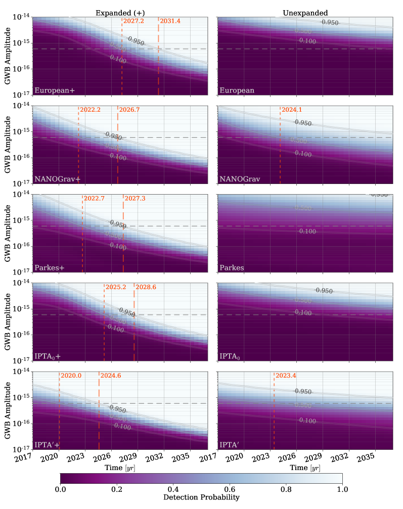
Figure 13: Detection Probability (DP) for purely power-law GWB spectra exploring different intrinsic GWB amplitudes over different observation durations for each PTA. The left column shows the expanded (‘+’) configurations where new pulsars are added each year, while the right column shows the static configurations with only the current number of pulsars. The IPTA₀ is the official specification for the International pulsar timing array, while the IPTA^′ is a more optimistic, manual combination of the specifications for each of the three individual PTA (see §2.4). The horizontal, dashed grey lines show the GWB amplitude from our fiducial model: $A_{\textrm{\tiny{yr}}^{-1}}=0.6\times\nobreak 10^{-15}$, and the vertical, dashed orange lines show the time at which each configuration reaches $\mathrm{DP}=50\%$ (short-dashes) and $\rm{DP}=95\%$ (long-dashes) for the fiducial amplitude. For a power-law spectrum at the fiducial amplitude, we expect IPTA^′+ to reach $50\%$ & $95\%$ DP in about 3 & 8 years ($\sim 2020$ & $\sim 2025$) respectively. Without expansion, the IPTA^′ reached $50\%$ DP in about 6 years ($\sim 2023$), and does not reach $95\%$ DP within 20 years.

To test our PTA configurations and detection statistics, we reproduce the results of Taylor et al. (2016, Fig. 2) for purely power-law GWB spectra. Our detection probabilities for each PTA are shown in Fig. 13. The left column shows expanded (+) arrays, with new pulsars added each year, while the right column shows the current array configurations. Our Detection Probabilities (DP) are close to those of Taylor et al. (2016), but not identical, likely due to differences between our noise scaling-factors $\lambda_{\textrm{noise}}$. Each panel has vertical lines denoting the year in which each PTA reaches $50\%$ (short-dashed) and $95\%$ DP (long-dashed). For these power-law GWB models at our fiducial ${A_{\textrm{\tiny{yr}}^{-1}}=0.6\times\nobreak 10^{-15}}$ (KBH-16), the individual PTA reach $95\%$ DP in roughly 2031, 2027 & 2027 for the EPTA+, NANOGrav+ & PPTA+ respectively. The IPTA₀+ reaches the same DP at 2029, while IPTA^′+ cuts that down to 2025. IPTA₀+ performing worse than NANOGrav and Parkes further motivates the usage of the IPTA^′+ model. The difference between static and expanding arrays is quite significant. For example, by 2037, none of the static PTA models reach $95\%$ DP. This highlights the importance of continuing to observe known pulsars, while also surveying the sky looking for new ones. Survey programs have been carried out by several large radio telescopes around the world, including GBT and Arecibo in the US, and their continued efforts and funding is of critical importance for PTA science.

3 Results

3.1 Eccentric Evolution

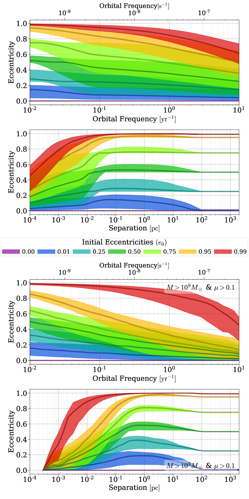
Figure 1: Evolution of eccentricity versus separation (panels a & c) and orbital frequency (panels b & d) for a variety of initial eccentricities. The upper panels (a & b) show eccentricities for all binaries, while the lower panels (c & d) show only the heavy ($M>10^{9}\,\textrm{M}_{\odot}$) and major ($\mu>0.1$) subset which tend to dominate the GWB. Each band corresponds to $68\%$ of the population, and the central lines to the medians.

For a given simulation, all binaries are initialized with the same eccentricity and are let to evolve with dynamical friction (DF), loss-cone (LC) stellar scattering, drag from a circumbinary Viscous-Disk (VD), and Gravitational Wave (GW) hardening. LC increases initially-nonzero eccentricities, and GW emission decreases them. In our models we assume DF & VD do not affect the eccentricity distribution. The upper panels of Fig. 1 show the resulting binary eccentricity evolution versus orbital frequency (a) and binary separation (b) for our entire population of MBHB. Solid lines show median values at each separation, and colored bands show the surrounding $68\%$. Binaries initialized to ${e_{0}=0.0}$ stay at zero, but the population initialized to only $e_{0}=0.01$ have a median roughly ten times larger at ${r\sim 1\,\mathrm{pc}}$, and still ${e\gtrsim 0.05}$ at orbital frequencies of $1\,\textrm{yr}^{-1}$.

Binaries which are both heavy ($M>10^{9}\,\textrm{M}_{\odot}$) and major ($\mu>0.1$) tend to dominate the GWB signal (Kelley et al., 2016). The eccentricity evolution of this subset of binaries is shown separately in panels (c) & (d) of Fig. 1. The eccentricities of these systems tend to dampen more quickly at separations below ${\sim}1\,\mathrm{pc}$. In general, this leads to much lower eccentricities at PTA frequencies for the heavy & major population. In the $e_{0}=0.95$ model, for example, the heavy & major median eccentricity drops below $0.6$ by ${f=0.1\,\textrm{yr}^{-1}}$ (panel c), whereas it takes until ${f\sim 3\,\textrm{yr}^{-1}}$ for the population of all binaries (panel a). In terms of separation, most of the ${e_{0}=0.95}$ population has ${e\lesssim 0.5}$ by ${r\sim 10^{-2}\,\mathrm{pc}}$, whereas for all binaries the same isn’t true until ${r\sim 10^{-4}\,\mathrm{pc}}$. The highest eccentricity model, ${e_{0}=0.99}$, behaves somewhat differently, as it tends to in many respects. For ${e_{0}=0.99}$, binaries pass through most of the PTA band before their eccentricities are substantially damped in both the overall and heavy & major groups.

Once binaries begin to approach the PTA sensitive band (${f\gtrsim 10^{-2}\,\textrm{yr}^{-1}}$) the eccentricity distributions are always monotonically decreasing. At the corresponding separations, GW becomes more and more dominant to LC, but at the same time, VD can still be an important hardening mechanism. If circumbinary disks can be effective at increasing eccentricity, or if a resonant third MBH were present, eccentricities could still be excited in the PTA regime. Either of these effects may be important for some MBHB systems, but likely not for the overall population.

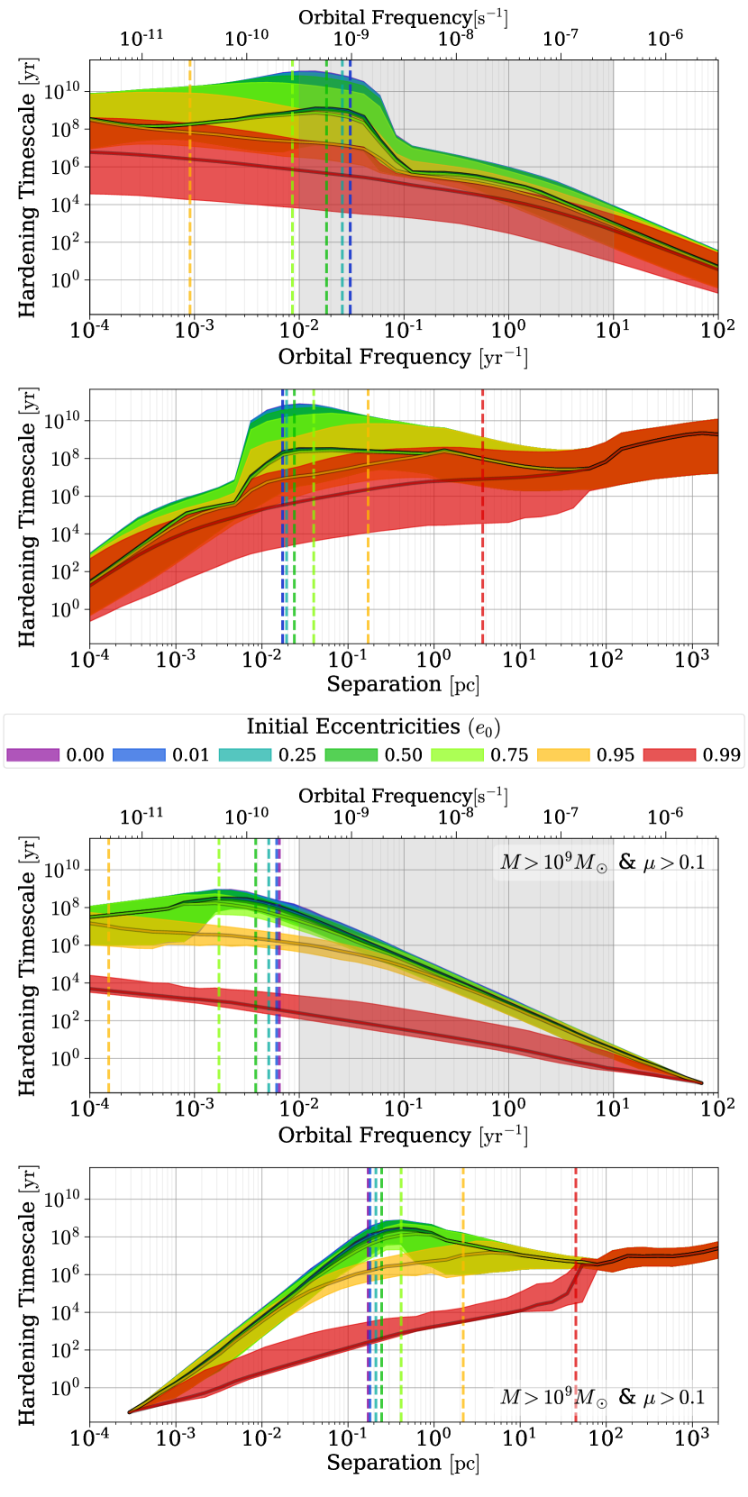
Figure 2: Binary hardening timescale ($a/(da/dt)$) against orbital frequency (panels a & c) and binary separation (panels b & d). Note that the frequency axes show an extended range, with the PTA-sensitive band shaded in grey. The upper panels (a & b) show hardening rates for all binaries, while the lower panels (c & d) show only the heavy & major subset. The dashed vertical lines indicate the radii at which GW-driven hardening becomes dominant over DF and LC.

In our models, while binary eccentricity is evolved by both LC and GW hardening, the eccentricity distribution itself only affects the rate of semi-major-axis hardening (i.e. $da/dt$, Eq. 3) by the GW mechanism. As eccentricity increases, GW hardening becomes more effective. The hardening time ($a/[da/dt]$) for all binaries is plotted in the upper panels of Fig. 2. The frequency panel (a) has been extended to show more of the physical picture, with the PTA-relevant regime shaded in grey. The DF regime goes from large separations down to ${r\sim 50\,\mathrm{pc}}$, and according to our prescription includes no eccentricity dependence.

The relatively flat portion of the hardening curve between ${r\sim 50\,\mathrm{pc}}$ and ${r\sim 2\times\nobreak 10^{-2}\,\mathrm{pc}}$ (panel b) is typically the LC-dominated regime. Ignoring the radial dependence of galactic $\rho/\sigma$ (density/velocity) profiles, the hardening rate should scale like ${\scalebox{1.2}{$\uptau$}_{\textrm{h}}\propto a^{-1}}$ (see Eq. 1). The hardening rates in panel b, however, show the combined binary evolutionary tracks over many orders of magnitude in total-mass and mass-ratio, flattening the hardening curves. The scaling is more clear for the low-eccentricity models of the heavy & major subset (panel d) which show more canonical LC hardening rates between ${r\sim 10\,\mathrm{pc}}$ and ${r\sim 1\,\mathrm{pc}}$.

Even at these large separations, the hardening timescale is significantly decreased for the highest initial eccentricities: ${e_{0}=0.95}$ and especially ${e_{0}=0.99}$. In these models, GW emission begins to play an important role in hardening much earlier in the systems’ evolution. The dashed vertical lines in Fig. 2 show the frequency and separation at which GW hardening becomes dominant over DF and LC in $50\%$ of systems. For ${e_{0}=0.99}$, GW domination occurs at a few parsecs, largely circumventing the LC regime entirely. As eccentricity decreases, so does the transition separation. For lower initial eccentricities, ${e_{0}\lesssim 0.75}$, the DF & LC become sub-dominant at a few times ${10^{-2}\,\mathrm{pc}}$, and the overall hardening rates are hardly distinguishable between different eccentricities.

Panels (c) & (d) of Fig. 2 show the hardening time for the population of heavy & major binaries. While very similar to the overall population, the heavy & major binaries are all effectively in the GW regime at frequencies ${f\gtrsim 10^{-2}\,\textrm{yr}^{-1}}$, i.e. the entire PTA band. In the ${e_{0}=0.0}$ model, binaries in the PTA-band show a nearly perfect power-law hardening rate from GW-evolution, and eccentricities ${e_{0}\lesssim 0.75}$ are hardly different. In the ${e_{0}=0.95}$ model, a heightened hardening rate is clearly apparent up to ${f\sim 10^{-1}\,\textrm{yr}^{-1}}$. The ${e_{0}=0.99}$ model evolves five orders of magnitude faster than ${e_{0}=0.0}$ at ${f=10^{-2}\,\textrm{yr}^{-1}}$, and still more than two orders faster even at ${f=1\,\textrm{yr}^{-1}}$. The ${e_{0}=0.99}$ model hardens drastically faster than the others both because of the strong eccentricity dependence of the GW hardening rate (Eq. 3) and because the eccentricity of the ${e_{0}=0.99}$ population better retains its high values at smaller separations.

At frequencies below $10^{-3}$–$10^{-2}\,\textrm{yr}^{-1}$ and lower eccentricity models (${e_{0}\lesssim 0.75}$), the heavy & major population is LC-dominated, causing sharp turnovers in the their hardening curves which is echoed in the resulting GWB spectra. In the population of all binaries (panel a) the transition occurs at slightly higher frequencies. The higher eccentricity models, which transition to GW domination at lower frequencies, do not show the same break in their hardening rate evolution. The resulting GWB spectra, however, still do (discussed in §3.2).

In all of our models, GW hardening is dominant to both dynamical friction and stellar scattering for the binaries which will dominate GWB production (heavy & major at ${f\gtrsim 10^{-2}\,\textrm{yr}^{-1}}$). Viscous drag, however, tends to be comparable or higher in much of the binary population. Deviations to the power-law index of hardening rates in the PTA regime are not apparent, however, because VD has a very similar radial dependence to GW emission (see §2.2). Although the GWB spectrum is only subtly affected by VD, the presence of significant gas accretion in the PTA band is promising for observing electromagnetic counterparts to GW sources, and even multi-messenger detections with ‘deterministic’/‘continuous’ GW-sources—those MBHB resolvable above the stochastic GWB (e.g. Sesana et al., 2012; Tanaka et al., 2012; Burke-Spolaor, 2013).

It should be clear from Fig. 2 that the hardening timescale is often very long (${\scalebox{1.2}{$\uptau$}_{\textrm{h}}\sim\scalebox{1.2}{$\uptau$}_{\textrm{Hubble}}}$) and varies significantly between binary systems. A substantial fraction of binaries, especially those with lower total mass and more extreme mass ratios, are unable to coalesce before redshift zero. The presence of significant eccentricity at sub-parsec scales can significantly decrease the hardening timescale, increasing the fraction of coalescing systems overall. The heavy & major subset of binaries, however, already tends to coalesce more effectively, and because this portion of the population dominates the GWB, its amplitude due to varying coalescing fractions is only subtly altered.

3.2 Gravitational Wave Backgrounds

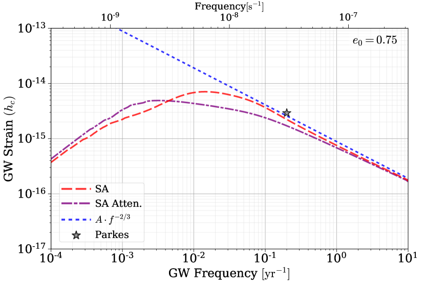
Figure 3: Stochastic Gravitational Wave Background calculated with the Semi-Analytic (SA) method, showing the effects of large binary eccentricities on the GWB spectrum. A purely power-law model is shown in the blue dotted line, which includes the masses and redshifts of merger events but assumes all energy is emitted in GW. The purple dot-dashed line includes the effect of attenuation from environmental hardening effects. The red dashed line shows the full SA calculation including both attenuation and the redistribution of GW energy across multiple frequencies. Note that this model uses a large initial eccentricity of $e_{0}=0.75$.

3.2.1 The Semi-Analytic GWB

The simplest calculation of the GWB assumes that all binaries coalesce effectively, quickly, and purely due to GW emission. This leads to a purely power-law strain spectrum, $h_{\textrm{\tiny{c, GW}}}\propto f^{-2/3}$. Environmental hardening, however, is required for the vast majority of binaries to be able to coalesce within a Hubble time. These additional hardening mechanisms also force binaries to pass through each frequency band faster than they otherwise would, decreasing the GW energy emitted in that band, and attenuating the GW background spectrum (e.g. Eq. 11, or Ravi et al., 2014).

Non-zero eccentricity increases the instantaneous GW luminosity and decreases the hardening time (Eq. 3). Also, the GW emission from eccentric binaries is no longer produced monochromatically at twice the orbital frequency, but instead is redistributed, primarily from lower to higher frequencies (Eq. 6). The effects of increased attenuation and the frequency redistribution are shown separately in Fig. 3 for ${e_{0}=0.75}$. The blue, dotted line shows a power-law spectrum (i.e. GW-only); while the purple, dashed-dotted line includes attenuation from the surrounding medium (predominantly LC-scattering). The red, dashed line includes the effects of chromatic GW emission, in addition to attenuation, which shifts the spectrum to higher frequencies. This is the full, semi-analytic (SA; §2.3.1) calculation. The spectral turnover is produced by the environmental attenuation, while the frequency redistribution slightly increases the amplitude in the PTA-regime (${f\gtrsim 10^{-2}\,\textrm{yr}^{-1}}$).

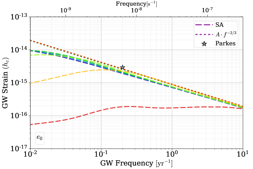
Figure 4: GWB strain spectrum calculate using the Semi-Analytic (SA) formalism for simulations with a range of initial eccentricities ($e_{0}$). The dotted lines assume purely GW-driven evolution and no frequency redistribution, and show amplitude increasing slightly with increasing $e_{0}$—because more systems coalesce. The dashed lines show the full SA calculation, including both attenuation and the frequency redistribution. Note that the power-laws (dotted) are not physically meaningful per se, and are meant as a reference when interpreting the SA models (dashed). For ${f\gtrsim 2\times\nobreak 10^{-1}\,\textrm{yr}^{-1}}$, the GWB amplitude increases with increasing $e_{0}$ until ${e_{0}=0.99}$, at which point the GWB amplitude is drastically depressed—almost completely flat—across the PTA band.

The GWB strain spectrum is shown for a variety of initial eccentricities in Fig. 4. Purely power-law spectra calculated assuming GW-only evolution are shown in dotted lines, while the full SA calculation is shown with dashed lines. The power-law spectra show a very slightly increasing GWB amplitude with increasing eccentricity as more binaries are able to coalesce before redshift zero. For initial eccentricities ${e_{0}\lesssim 0.5}$, the GWB spectrum above frequencies ${f\gtrsim 10^{-2}\,\textrm{yr}^{-1}}$ are nearly identical. For higher initial values, the effects of non-zero eccentricity become more apparent. Overall, for all but the highest eccentricities ($e_{0}>0.9$), the effect of non-circular orbits is actually to slightly increase the GWB amplitude in the PTA frequency band, because of the redistribution of GW energy to higher harmonics. Note that this is because the spectral turnover is always below the PTA-band in our spectra (also seen in, e.g., Chen et al., 2016). If galactic densities are significantly larger than those found in the Illustris simulations, the environment could continue dominating binary evolution to higher frequencies. If that were the case, the spectral turnover could be within the PTA band which would lead to chromatic GW emission decreasing the observable signal. In appendix §B, we include additional information on binary host-galaxy densities from Illustris.

In the highest eccentricity case (${e_{0}=0.99}$; red lines), binaries are still highly eccentric at separations corresponding to frequencies all the way up to ${f\sim 10\,\textrm{yr}^{-1}}$, and the GWB amplitude is drastically diminished throughout the PTA band. While such high eccentricities may be unlikely (e.g. Armitage & Natarajan, 2005; Roedig et al., 2011), having some subset of the population maintain high eccentricities into the PTA band is certainly not impossible (e.g. Rantala et al., 2016). If Kozai-Lidov-like processes from a hierarchical, third MBH were driving the eccentricity (e.g. Hoffman & Loeb, 2007; Bonetti et al., 2016), or the binary were counter-rotating to the stellar core or circumbinary disk (e.g. Sesana et al., 2011; Amaro-Seoane et al., 2016), eccentricities could grow much faster than in our results. Better understanding what fraction of systems could be susceptible to these processes is an important direction of future study.

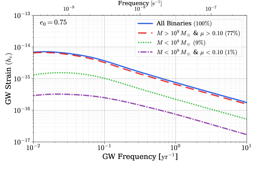
Figure 5: GWB from different binary subsets selected by total mass $M$, and mass ratio $\mu$. The blue (solid) line shows the total GWB from all binaries, while the red (dashed) line shows the contribution from heavy & major systems (shown also in Figs. 1 & 2). Light systems (green, dotted) and light & minor binaries (purple, dot-dashed) are also shown. The percentages in the legend show the contribution to the GWB energy at $1\,\textrm{yr}^{-1}$ (i.e. ${\propto h_{\textrm{\tiny{c}}}^{2}(f=1\,\textrm{yr}^{-1})}$) for each subgroup. Here, the heavy & major subgroup, while only $1\%$ of binaries by number, contributes almost $80\%$ of the GWB energy.

The contribution the GWB is broken down by subgroups of total mass and mass ratio in Fig. 5. The complete GWB is shown in blue (solid), while the heavy & major subset is in red (dashed), the light (${M<10^{9}\,\textrm{M}_{\odot}}$) in green (dotted), and the light & minor (${\mu<0.1}$) in purple (dash-dotted). The heavy & major binaries are only $\sim 1\%$ of the population, but here, in the $e_{0}=0.75$ model, contribute $\sim 80\%$ of the GWB energy density at $1\,\textrm{yr}^{-1}$. In fact, heavy & major systems dominate at all frequencies with a very similar spectral shape to the overall GWB, with a slight enhancement of GW strain at lower frequencies. Lower-mass binaries ($M<10^{9}\,\textrm{M}_{\odot}$) contribute less than $10\%$ of the energy (despite being just over $90\%$ of the population), and systems which are neither heavy nor massive contribute only $1\%$ ($\sim 30\%$ of the population). Other initial eccentricity models tend to be even more heavy & major dominated (often $\sim 90\%$).

3.2.2 The Monte-Carlo GWB

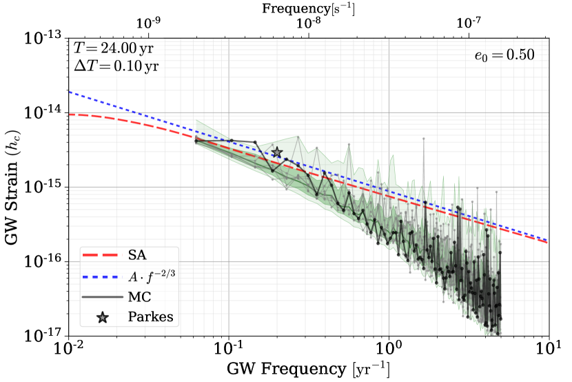
Figure 6: GWB calculated using the Monte-Carlo (MC) method, for a simulation with initial eccentricities ${e_{0}=0.5}$. Seven different GWB realizations are shown in gray and black lines, while the median and one- & two- sigma contours are shown in green. Semi-Analytic (SA) calculations are also shown: purely power-law in blue (dotted), and full in red (dashed). The high frequency spectrum of the MC calculation is sharper than that of the SA methods due to quantization of binaries.

The Monte-Carlo (MC) approach (§2.3.2) to calculating the GWB dispenses with the continuum approximation for the density of GW sources, thereby allowing for the quantization of MBHB at the same time as providing a convenient formalism for constructing an arbitrary number of realizations from the same binary population. The MC GWB is shown in Fig. 6, with seven randomly-chosen realizations plotted in gray and black. The median line and one- & two- sigma contours of 200 realizations are shown in green. For reference, the SA spectra are shown for purely power-law calculations (blue, dotted) and the full SA (red, dashed). The frequency bins correspond to Nyquist sampling at a cadence $\Delta T=0.1\,\mathrm{yr}$, and total observational-duration $T=24\,\mathrm{yr}$.

The MC GWB differs from the SA one, both in its jaggedness and also in a steeper spectrum at higher frequencies. The jaggedness is caused by varying numbers of binaries in the observer’s past light cone (Eq. 16)—especially massive ones at lower redshifts. The latter effect is due to binary quantization: at high frequencies, where the hardening time is short, there are few MBHB contributing to each frequency bin. The SA calculation, however, implicitly includes the contribution from fractional binaries, artificially inflating the GWB amplitude at high frequencies (Sesana et al., 2008).

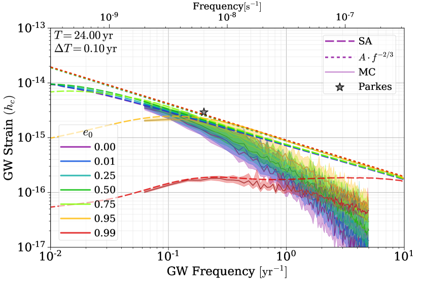
Figure 7: Monte-Carlo (MC) calculated GWB for a variety of different initial eccentricities ($e_{0}$). Median lines and one-sigma contours are shown for the MC case, and both the full (dashed) and power-law (dotted) SA calculations are also shown. Increasing GWB amplitude with increasing eccentricity is apparent at lower frequencies (${\sim 10^{-1}\,\textrm{yr}^{-1}}$, until the spectrum turns over. While the spectral turnover is produced by environmental interaction, the frequency at which it occurs is increased with rising eccentricity. At higher frequencies (${\gtrsim 2\times\nobreak 10^{-1}\,\textrm{yr}^{-1}}$), as eccentricity increases, the MC results come closer and closer to the SA ones due to additional binaries at lower orbital frequencies contribute to higher GW-frequency bins.

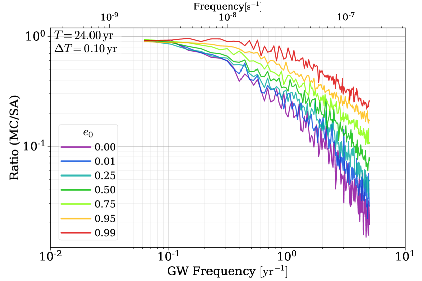
Figure 14: Ratio of the (median) MC-calculated GWB to that of the SA calculation. Binaries at higher eccentricities contribute more GW energy to higher-harmonics above their orbital frequency. This causes the number of sources contributing at higher-frequencies to increase with increasing eccentricity, decreasing the effects of MBHB quantization.

Figure 7 shows the GWB for a variety of initial eccentricities, with median lines and one-sigma contours for the MC calculation, along with the full and power-law SA calculations. Both the SA and MC methods show slightly increased GWB amplitudes with increasing eccentricities (except for the highest, $e_{0}=0.99$ simulation). A more pronounced effect is that the higher the eccentricity, the closer the high-frequency portion of the MC calculation comes to the purely power-law spectra. The ratio of the MC GWB (median lines) to SA GWB is shown explicitly in Fig. 14. Higher eccentricities mean that GW energy from binaries at lower orbital-frequencies are deposited in higher GW-frequency bins. This means that overall, more binaries are contributing to each of the higher frequency bins, reducing the effect of MBHB quantization, and thus bringing the MC results closer in line to the SA models. Finite-number effects at high frequencies are also remediated by increased numbers of coalescing systems, as is the case for very large LC refilling fractions ($\mathcal{F}_{\textrm{\tiny{refill}}}$), for example, shown in Figs. 15 & 16.

3.3 Pulsar Timing Array Detections

3.3.1 Eccentric Binary Evolution

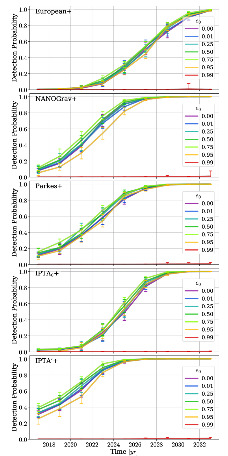
Figure 8: Detection Probability (DP) versus time for eccentric evolution models with different initial eccentricities ($e_{0}$, colors) and different PTA (rows). The lines and error bars are averages and standard deviations over 200 MC realizations. Currently, in 2017, we find detection probabilities are below $20\%$ for all official PTA, but reach $95\%$ between about 2025 and 2032. Higher eccentricities tend to be slightly more detectable, until $e_{0}>0.75$ where the spectral turnover takes a toll on the low-frequency GWB amplitude.

Detection probability versus time are shown for eccentric-evolution models in Fig. 8 using expanded PTA configurations. Averages and standard deviations over 200 MC realizations are plotted. Ignoring the highest eccentricity case (${e_{0}=0.99}$), for the moment, the variation between different eccentricities is $\lesssim 20\%$ in DP, and generally ${\sim}2$ yr at a fixed value. The different DP growth curves are quite similar between PTA, with DP tending to be higher for higher eccentricities between ${e_{0}=0.0}$ and ${e_{0}=0.75}$. Not surprisingly, the ${e_{0}=0.99}$ model is an outlier in DP as in binary evolution. In this extreme case the GWB is effectively undetectable for all PTA.

The PTA differ in their response to the ${e_{0}=0.95}$ simulations depending on their frequency sensitivities. Longer observing durations mean PTA are able to detect lower frequencies, and the lowest accessible frequency bins are the most sensitive (see, e.g., Moore et al., 2015). Pulsars (and PTA) with the longest observing durations (i.e. Parkes) are most sensitive to the GWB spectral turnover accentuated in the high eccentricity models. As observing time increases, however, sensitivity increases at all frequencies, and the addition of short duration (and low noise) expansion pulsars boosts high-frequency sensitivity. After a sufficient observing time, the high frequency portion of the GWB spectrum, where ${e_{0}=0.95}$ is highest (see Fig. 7), gains enough leverage for its DP to overtake that of lower eccentricities.

In Fig. 8, the IPTA₀+ doesn’t perform as well as Parkes+ at early times. This is due both to I) the differing noise calibrations—the IPTA₀’s white-noise is pushed significantly higher than Parkes to match the observed upper-limits, as well as, II) the specifications for each individual PTA not quite matching those included in the IPTA public specifications. Both of these factors motivate our inclusion of the IPTA^′ model, which has a higher DP than Parkes, even at early times, as expected. We are optimistic that future IPTA results and data releases will show even greater improvements than suggested by those of the initial IPTA.

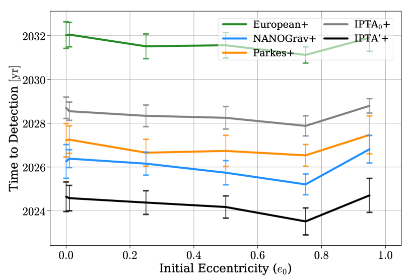
Figure 9: Time to reach a $95\%$ DP versus initial eccentricity ($e_{0}$) of MBH binaries. Each (expanded, ‘+’) PTA is shown with the average and standard deviation of 200 MC realizations. While the official IPTA₀ specification lags behind Parkes and NANOGrav, the more optimistic IPTA^′ model reaches $95\%$ DP almost two years earlier.

Figure 9 shows times to reach $95\%$ DP versus initial eccentricity for each PTA. Overall, time to detection tends to improve slightly with increasing eccentricity as it increases the GWB amplitude in the mid-to-upper PTA band. Differences between eccentricities, however, tend to be comparable or smaller than the variance between MC realizations. For very high eccentricities, ${e_{0}>0.75}$, the time to detection again increases as the GWB spectral turnover becomes ‘visible’ to PTA, and the signal is diminished. While the ${e_{0}=0.99}$ models never reach $95\%$ DP in our results, additional simulations of a ‘rapid’ IPTA^′+ model, where expansion pulsars have a cadence of 2 days (see §D, ‘ IPTA${}^{\prime}_{\mathrm{rap}}$ ’), are able to reach DP $\sim 50\%$ by 2032. Even in the highest eccentricity model with ${e_{0}=0.99}$, detection prospects for individual, deterministic sources may not be affected quite as strongly. We are currently exploring single source predictions from our models, to be presented in a future study.

3.3.2 Circular Binary Evolution

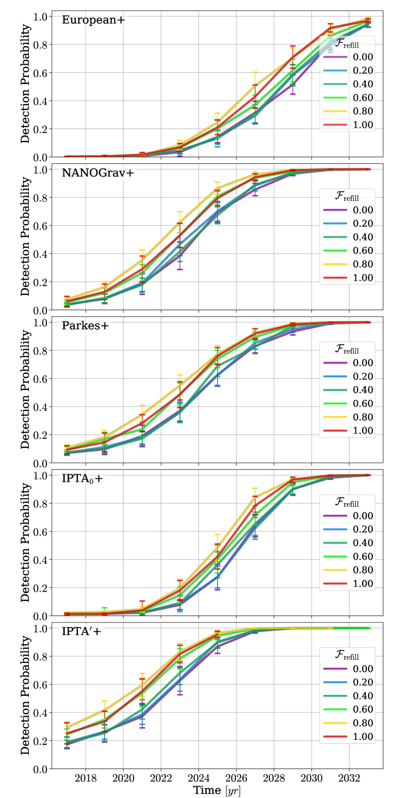
Figure 10: DP versus time for circular evolution models with different LC efficiencies ($\mathcal{F}_{\textrm{\tiny{refill}}}$, colors) and different expanded PTA (rows). These growth curves behave very similarly to those of the eccentric models, but generally take ${\sim}2$ yr longer to reach the same DP. There is also a stronger trend across $\mathcal{F}_{\textrm{\tiny{refill}}}$ compared to $e_{0}$, with ${\mathcal{F}_{\textrm{\tiny{refill}}}=0.0}$ reaching the same DP ${\sim}2$ yr slower than for ${\mathcal{F}_{\textrm{\tiny{refill}}}\sim 0.8}$ – $1.0$.

Detection probability versus time for circular evolution models with a variety of loss-cone refilling parameters ($\mathcal{F}_{\textrm{\tiny{refill}}}$) are shown in Fig. 10. Recall that a low, ‘steady-state LC’ corresponds to ${\mathcal{F}_{\textrm{\tiny{refill}}}=0.0}$, and a highly effective, ‘full LC’ to ${\mathcal{F}_{\textrm{\tiny{refill}}}=1.0}$. Overall a similar range of durations are required for comparable DP, but the circular models are systematically harder to detect, taking roughly $2$ years longer. This is not surprising as the eccentric models assume a full LC, and increasing eccentricity tends to further enhance the GWB amplitude in the PTA band. In general, higher $\mathcal{F}_{\textrm{\tiny{refill}}}$ lead to higher DP after a fixed time. The circular, full LC, tends to have a slightly lower DP as the attenuation and spectral turnover from stellar scattering take effect, analogous to the highest eccentricities (see, e.g., Fig. 15). The IPTA^′+ model shows a slight improvement in time to detection between ${\mathcal{F}_{\textrm{\tiny{refill}}}=0.8}$ and ${\mathcal{F}_{\textrm{\tiny{refill}}}=1.0}$, suggesting that its high-frequency sensitivity is able to win out.

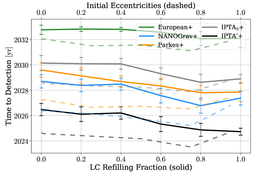
Figure 11: Time to reach a $95\%$ DP versus LC refilling fraction ($\mathcal{F}_{\textrm{\tiny{refill}}}$; solid lines) for circular binary-evolution models. The times to detection for varying eccentricity models (from Fig. 9) are overplotted (dashed lines) for comparison. Averages and standard deviations are shown. Varying $\mathcal{F}_{\textrm{\tiny{refill}}}$ has a pronounced effect on detection times, with more effective scattering (larger $\mathcal{F}_{\textrm{\tiny{refill}}}$) models taking less time to observe. Because the eccentric evolution models assume a full loss-cone, the ${\mathcal{F}_{\textrm{\tiny{refill}}}<1.0}$ models tend to take longer to be detected.

Figure 11 summarizes the circular-evolution times to detection for each PTA versus $\mathcal{F}_{\textrm{\tiny{refill}}}$ (solid lines). Overplotted are the eccentric-evolution times to detection (dashed lines, upper x-axis) for comparison. Based on these trends, a population of MBHB with very high LC scattering efficiency ($\mathcal{F}_{\textrm{\tiny{refill}}}\sim 0.8-1.0$) and intermediate eccentricities $0.5<e_{0}<0.8$ would be the easiest to detect.

4 Conclusions

This paper has focused on plausible detections of a stochastic Gravitational Wave Background (GWB) using Pulsar Timing Arrays (PTA). We have expanded on the Massive Black-Hole (MBH) merger models presented in Kelley et al. (2016) based on the Illustris simulations. We have added a model for eccentric binary evolution assuming ‘full’ Loss-Cone (LC) stellar scattering, in addition to our existing prescriptions for dynamical friction, stellar scattering with a variety of LC efficiencies ($\mathcal{F}_{\textrm{\tiny{refill}}}$), viscous drag from a circumbinary disk, and Gravitational Wave (GW) emission. We have run sets of simulations with a variety of LC efficiencies and initial (at the start of stellar scattering) eccentricities. The MBH binary evolution produced by our models is explored along with Monte-Carlo (MC) realizations of the resulting stochastic GW Background (GWB) spectra. Using parametrized models of currently operational PTA, and their future expansion, we calculate realistic prospects for detections of the GWB.

The presence of non-zero eccentricity causes two distinct effects to MBH Binary (MBHB) evolution and their GW spectra. First, increased eccentricity causes faster GW-hardening and thus more binary coalescence, but there is additional attenuation of the GWB spectrum and a stronger spectral turnover at low frequencies. Second, while circular binaries emit GW at only twice the orbital frequency (the $n=2$ harmonic), eccentric binaries also emit at all higher harmonics (and the $n=1$). The total GW energy released remains the same, but the overall effect is to move GW energy from lower to higher frequencies (Fig. 3).

GWB spectra constructed using a Semi-Analytic (SA) calculation (Fig. 4) show that the amplitude ($A_{\textrm{\tiny{yr}}^{-1}}$) of the GWB near the middle of the PTA band ($f\sim 1\,\textrm{yr}^{-1}$) tends to increase with increasing eccentricity up to $e_{0}=0.95$. This is due primarily to the first eccentric effect: with hardening more effective, the number of binaries coalescing by redshift zero increases. At lower frequencies, environmental effects—specifically stellar scattering—produce a strong turnover in the GWB spectrum. Even moderate eccentricities begin to increase the frequency at which this turnover occurs because of the second eccentric effect. Unless the population of binaries dominating the GWB have very high eccentricities ($e\gtrsim 0.8$), the spectral turnover remains below the PTA sensitive band ($f\lesssim 0.02\,\textrm{yr}^{-1}$).

The location of the spectral turnover in our models differs from those predictioned by Ravi et al. (2014) who see the turnover at frequencies as high as $f\sim 10^{-1}\,\textrm{yr}^{-1}$. The location of the turnover depends on the strength of environmental factors, and thus galactic density profiles. If the stellar densities of massive-MBHB host-galaxies are higher than predicted by Illustris, the turnover could occur at PTA-observable frequencies, regardless of (or exaggerated by) eccentricity distribution. If the turnover does exist in the current PTA band, it could hurt detection prospects. At the same time, observations of such a turnover would be uniquely indicative of environmental interactions, while observations of the GWB amplitude overall are highly degenerate between cosmological factors (i.e. the rate of binary formation) and environmental factors (determining the rate of binary coalescence). Currently PTA upper limits of the GWB are still entirely consistent with our results, and thus are unable to constrain or select between them.

GWB spectra constructed using the MC calculation (Fig. 7), which should resemble real signals, tend to have much steeper strain spectra than $-2/3$ at current PTA frequencies (${f\gtrsim 0.1\,\textrm{yr}^{-1}}$). This is because the number of binaries in each frequency bin becomes small, and binary quantization must be taken into account. MC realizations reveal an interesting corollary to the redistribution of GW energy: with non-zero eccentricity, a larger number of binaries at lower orbital-frequencies contribute to the GWB signal at higher observed-frequency bins. This softens the effect of binary quantization and the GWB spectra tend to come closer and closer to a $-2/3$ spectral index with increasing eccentricity (Fig. 14)—thus producing higher $A_{\textrm{\tiny{yr}}^{-1}}$. For example, the ${e_{0}=0.5}$ & ${e_{0}=0.95}$ models have $A_{\textrm{\tiny{yr}}^{-1}}$, 2 & 3 times larger than that of the ${e_{0}=0.0}$ model.

To calculate realistic detection statistics, we use parametrized version of each operational PTA: the European (EPTA), NANOGrav, Parkes (PPTA), and International (IPTA; a joint effort of the individual three). For the IPTA we consider both the public data specifications, IPTA₀; in addition to a more optimistic, manual combination of the individual groups, IPTA^′. Overall, our models for NANOGrav, Parkes, and IPTA₀ each behave comparably, reaching $95\%$ detection probability (DP) between 2026 and 2030, and the EPTA following 2 – 4 years later. The IPTA^′ model noticeably outperforms the others, reaching $95\%$ DP between 2024 and 2026. High cadence observations of IPTA^′ pulsars can further decrease time-to-detection by another $\sim 2$ years. Moderately high eccentricities ($0.5\lesssim e_{0}\lesssim 0.8$) tend to produce the largest GWB amplitudes in the PTA band. The eccentricity models used here assume a full loss-cone (LC; $\mathcal{F}_{\textrm{\tiny{refill}}}\approx 1.0$), and thus circular evolution models which decrease the LC refilling efficiency tend to have lower GWB amplitudes, and longer times to detection by up to $\sim 2$ years. If galactic-nuclear stellar densities are significantly higher than suggested by Illustris, and the LC is also nearly full, then attenuation of the GWB spectrum could increase times to detection.

Increased eccentricity tends to increase the GWB amplitude, and thus detection prospects. In the most extreme ${e_{0}=0.99}$ model, however, the signal is so drastically diminished that detections seem unlikely within 20 years in all but the high-cadence IPTA model. While eccentricities as high as $0.99$ may not be representative of the overall population of binaries, mechanisms which can preferentially drive more massive systems to higher eccentricities (e.g. counter-rotating stars/gas, Khan et al., 2011; Amaro-Seoane et al., 2016, or three-body resonances) should be further studied. Varying the eccentricity distribution of binaries has a strong effect on the strain spectral-index of the GWB at high frequencies ($f\gtrsim 1\,\textrm{yr}^{-1}$). While PTA are less sensitive at higher frequencies, eventual observations with high signal-to-noise could be used to constrain the underlying binary eccentricity distribution. The true eccentricity distribution will also affect the prospects for observations of individual, resolvable binaries (‘deterministic’/‘continuous’ sources)—a study of which is currently in progress.

As discussed above, the high frequency portion of the GWB spectrum that PTA will eventually observe is strongly influenced by individual MBHB sources. In effect, the high frequency portion of the spectrum is no longer a ‘background’. It has been shown that this leads to non-Gaussian signal statistics (Ravi et al., 2012) which are at odds with the assumptions of the detection statistics we use. Recently, Cornish & Sampson (2016) have found the standard analyses to be robust against small numbers of GW sources. None the less, if this effect were to systematically decrease GWB detection probabilities, it is likely the effect would be minor because: 1) detection probability is primarily driven at low-frequencies where individual sources are much less important; and 2) the Monte Carlo realization of the spectra we construct should be representative of variations in the GW background (neglecting single-sources), and thus our DP and time-to-detection error bars should still be representative.

For a given PTA configuration, the differences in times-to-detection for varying GWB model parameters are at most a few years. This result is promising as it suggests that, despite uncertainties in the underlying physical processes of binary mergers, the expectation of GWB detections in the near future remains robust. At the same time it begs the question, ‘will PTA be able to discern between different models in their observations?’ Based only on the overall GWB amplitude (or equivalently the time-to-detection), only a mixed measurement of the overall merger process and the typical MBH binary mass distribution will be constrained. The different hardening models are largely degenerate in the overall GWB amplitude they predict, especially when taking into account uncertainties in cosmological factors—most notably the true, unbiased distribution of MBH masses (e.g. Shen et al., 2008; Shankar et al., 2016)—which is outside of the scope of this study.

Once PTA have detected the GWB, and signal-to-noise continues to grow, the shape of the GWB will be measured which encodes very detailed information about the merger process and typical MBH environments (e.g. Taylor et al., 2017; Chen et al., 2017). The strength of the (low-frequency) spectral turnover is determined by the MBHB coupling to their local stellar environments, and its location is additionally effected by the eccentricity distribution of binaries. The (high-frequency) spectral-index, however, measures the number of sources contributing to the GWB, and thus the underlying eccentricity distribution. In the ideal, high signal-to-noise regime, the spectral index will determine typical binary eccentricities which can then be disentangled from the stellar coupling, measured from the spectral turnover. With eccentricity and the loss-cone constrained, the typical masses of merging MBHB can then be inferred from the overall GWB amplitude.

Low frequency sensitivity, established by long observing baselines, tends to drive increases in detection probability. Still, we find that including short cadence observations to maintain or improve high frequency sensitivity can make a noticeable difference in detection prospects, especially for the most extreme hardening and eccentricity models (in which the GWB spectra turn over at low frequencies). Regardless of cadence, we find that the continued addition of pulsars monitored by PTA is essential for a detection to be made within the next 20 years. Across a wide range of specific configurations, and even with pessimistic model parameters, if PTA continue to expand as they are, GWB detections are highly likely within about 10 years.

Appendix A Additional Equations

The GW frequency distribution function can be expressed as (Peters & Mathews, 1963, Eq. 20),

$$\begin{gathered}g(n,e)\equiv\frac{n^{4}}{32}\left(\left[G_{1}\vphantom{e^{2}}\right]^{2}+\left[1-e^{2}\right]\left[G_{2}\vphantom{e^{2}}\right]^{2}+\frac{4}{3n^{2}}\left[J_{n}(ne)\vphantom{e^{2}}\right]^{2}\right),\\ G_{1}(n,e)\equiv J_{n-2}(ne)-2eJ_{n-1}(ne)+\frac{2}{n}J_{n}(ne)+2eJ_{n+1}(ne)-J_{n+2}(ne)\vphantom{\frac{2}{n}},\\ G_{2}(n,e)\equiv J_{n-2}(ne)-2eJ_{n}(ne)+J_{n+2}(ne)\vphantom{\frac{2}{n}}.\end{gathered}$$ (19)

Here $J_{n}(x)$ is the n’th Bessel Function of the first kind. The sum of all harmonics, ${\sum_{n=1}^{\infty}g(n,e)=F(e)}$, where $F(e)$ is defined in Eq. 4.

The observed, characteristic strain from a set of individual sources is (e.g. Rosado et al., 2015, Eq. 8),

$$h_{\textrm{\tiny{c}}}^{2}=\sum_{i}h_{\textrm{\tiny{s,i}}}^{2}\,\frac{f_{i}}{\Delta f}\approx\sum_{i}h_{\textrm{\tiny{s,i}}}^{2}\,f_{i}\,T,$$ (20)

where the second equality assumes that frequency bins are determined by the resolution corresponding to a total observational duration $T$.

The cosmological evolution function is (Hogg, 1999, Eq. 14),

$$E(z)\equiv\sqrt{\Omega_{\rm M}\,(1+z)^{3}+\Omega_{k}\,(1+z)^{2}+\Omega_{\Lambda}},$$ (21)

for $z$ the redshift, and $\Omega_{\rm M}$, $\Omega_{k}$ & $\Omega_{\Lambda}$ the density parameters for matter, curvature and dark-energy.

A.1 Detection Formalism

In what follows, the GWB signal is characterized by a Spectral Energy Density (SED),

$$S_{h}=\frac{h_{c}^{2}}{12\pi^{2}f^{3}},$$ (22)

and the prediction/model SED is denoted as $S_{h0}$. In all of our calculations, we use a purely power-law GWB spectrum for $S_{h0}$ with an amplitude of $A_{\textrm{\tiny{yr}}^{-1}}=10^{-16}$. Each pulsar $i$ is characterized by a noise SED $P_{i}$ (Eq. 18).

PTA detection statistics typically rely on cross-correlations between signals using an ‘overlap reduction function’ (the Hellings & Downs, 1983, curve),

$$\Gamma_{ij}=\frac{3}{2}\gamma_{ij}\,\ln\left(\gamma_{ij}\right)-\frac{1}{4}\gamma_{ij}+\frac{1}{2}+\frac{1}{2}\delta_{ij}$$ (23)

where,

$$\gamma_{ij}=\frac{1}{2}\left[1-\cos(\theta_{ij})\right],$$ (24)

for an angle between pulsars $i$ and $j$, $\theta_{ij}$.

We employ the ‘B-Statistic’ from Rosado et al. (2015), constructed by maximizing the statistic’s SNR—defined as the expectation value of the statistic in the presence of a signal,

$$\mu_{B1}=2\sum_{k}\sum_{ij}\frac{\Gamma_{ij}^{2}\,S_{h}\,S_{h0}}{\left(P_{i}+S_{h0}\right)\left(P_{j}+S_{h0}\right)+\Gamma_{ij}^{2}\,S_{h0}^{2}},$$ (25)

divided by the variance of the statistic also in the presence of a signal,

$$\sigma_{B1}^{2}=2\sum_{k}\sum_{ij}\frac{\Gamma_{ij}^{2}\,S_{h0}^{2}\left[\left(P_{i}+S_{h}\right)\left(P_{j}+S_{h}\right)+\Gamma_{ij}^{2}\,S_{h}^{2}\right]}{\left[{\left(P_{i}+S_{h0}\right)\left(P_{j}+S_{h0}\right)+\Gamma_{ij}^{2}\,S_{h0}^{2}}\right]^{2}},$$ (26)

i.e. $\textrm{S}/\textrm{N}_{B}\equiv\mu_{B1}/\sigma_{B1}$, as apposed to the variance in the absence of a signal,

$$\sigma_{B0}^{2}=2\sum_{k}\sum_{ij}\frac{\Gamma_{ij}^{2}\,S_{h0}^{2}P_{i}\,P_{j}}{\left[{\left(P_{i}+S_{h0}\right)\left(P_{j}+S_{h0}\right)+\Gamma_{ij}^{2}\,S_{h0}^{2}}\right]^{2}}.$$ (27)

The SNR can then be expressed as,

$$\textrm{S}/\textrm{N}^{2}=\textrm{S}/\textrm{N}_{B}^{2}=2\sum_{k}\sum_{ij}\frac{\Gamma_{ij}^{2}\,S_{h}^{2}}{P_{i}P_{j}+S_{h}\left(P_{i}+P_{j}\right)+S_{h}^{2}\left(1+\Gamma_{ij}^{2}\right)},$$ (28)

which is only meaningful compared to the threshold-SNR for a particular false-alarm probability ($\alpha_{0}$) and DP-threshold ($\gamma_{0}$),

$$\textrm{S}/\textrm{N}_{B}^{T}=\sqrt{2}\left[\frac{\sigma_{0}}{\sigma_{1}}\mathrm{erfc}^{-1}\left(2\alpha_{0}\right)-\mathrm{erfc}^{-1}\left(2\gamma_{0}\right)\right].$$ (29)

The SNR can be circumvented altogether by considering the measured DP,

$$\gamma_{B}=\frac{1}{2}\mathrm{erfc}\left(\frac{\sqrt{2}\,\sigma_{0}\mathrm{erfc}^{-1}\left(2\alpha_{0}\right)-\mu_{1}}{\sqrt{2}\,\sigma_{1}}\right),$$ (30)

which is the primary metric we use throughout our analysis of PTA detections.

Appendix B Host-Galaxy Densities in Illustris

The point at which two MBH come within a smoothing length of one another is identified in Illustris, and density profiles are calculated for the host galaxy at that time. The profiles are used to calculate the environmental hardening rates which then determine the GWB spectra. In particular, the stellar densities strongly affect the location of the spectral turnover through stellar scattering. Because the location of the spectral turnover is especially important for future detections of the GWB, we provide some additional details on the stellar environments here.

To calculate density profiles, we average the density of each particle type (star, dark matter, and gas) in radial bins. Because Illustris is only able to resolve down to 10s–100s of parsec scales, we extrapolate to smaller radii with power-law fits to the eight inner-most bins. Fig. 12 shows the distribution of stellar densities at 10 pc (interpolated or extrapolated as needed) in the upper-panel, and power-law indices in the lower-panel. The overall population of binaries are shown in grey (dashed), in addition to the heavy ($M>10^{9}\,\textrm{M}_{\odot}$) subset in blue, and heavy & major ($\mu>0.1$) mass-ratio subset in red. There is a roughly 100 times increase in typical stellar densities between heavy systems and overall host-galaxies, but no noticeable change when further selecting by mass-ratio. While the heavy subset constitutes less than $10\%$ of systems, they contribute ${\sim}90\%$ of the GWB amplitude (see, KBH-16, ).

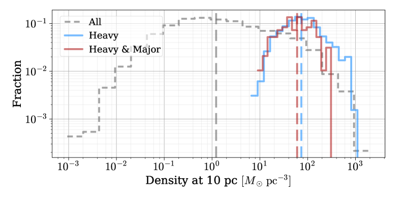
(a)

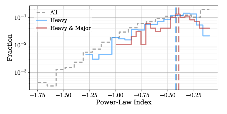
(b)

Figure 12: Upper-panel: distribution of stellar densities at $10\,\mathrm{pc}$ for Illustris galaxies hosting MBH binaries. For galaxies in which $10\,\mathrm{pc}$ is unresolved, the density is calculated from power-law fits to the inner-most (resolved) regions. The dashed grey lines show the entire population of binary host galaxies, while the blue lines show hosts of heavy ($M>10^{9}\,\textrm{M}_{\odot}$) binaries, and red the heavy and major ($\mu>0.1$) binaries. Each population is plotted fractionally, but note that heavy binaries constitute ${\sim}7\%$ and heavy & major ${\sim}1\%$ of all binaries respectively. Vertical lines indicate the median value of each subset.

The median power-law index for the inner stellar density profiles is ${\sim}-0.4$. For comparison, at small radii an Hernquist (1990) profile corresponds to $-1$, and $-1.5$ produces a surface-density distribution that resembles a de Vaucouleurs (1948) profile (Dehnen, 1993). At the same time, many massive galaxies (comparable to our host galaxies) have flattened ‘cores‘ in their stellar density profiles (e.g. Faber et al., 1997; Lauer et al., 2007) and it has long been proposed that these cores could be explained by dynamical scouring from MBH binaries (e.g. Quinlan & Hernquist, 1997; Volonteri et al., 2003). Both computationally and observationally, inner density profiles in the ‘hard’ binary regime (typically ${r\lesssim 10\,\mathrm{pc}}$) are very difficult to resolve. It is thus unclear how accurate these profiles are. While they may be realistic models, some of the flattening in the inner regions may be due in part to numerical effects (e.g. gravitational softening in the force calculations) or the known, over-inflated radii of some galaxies in Illustris (Snyder et al., 2015; Kelley et al., 2016).

Appendix C Additional Figures

Figure 15: Monte-Carlo (MC) calculated GWB for a variety of different LC refilling fractions ($\mathcal{F}_{\textrm{\tiny{refill}}}$), with median lines (solid) and one-sigma contours shown. Both the full (dashed) and power-law (dotted) SA models are also plotted. More efficient LC refilling means more binaries coalesce, causing the GWB amplitude to increase. An always full LC causes increased attenuation at lower frequencies: apparent at $f\lesssim 0.1\,\textrm{yr}^{-1}$. The steepening of the spectral index at higher frequencies due to finite-number effects is also apparent, but for $\mathcal{F}_{\textrm{\tiny{refill}}}>=0.8$, the effect is somewhat remediated.

Figure 16: Ratio of the (median) MC-calculated GWB to that of the SA calculation, for zero-eccentricity and a variety of LC refilling fractions ($\mathcal{F}_{\textrm{\tiny{refill}}}$). Finite-number effects, from few binaries in each bin, cause the strong deviation between Semi-Analytic (SA) and MC calculations at higher frequencies. This effect is somewhat alleviated by effective LC refilling ($\mathcal{F}_{\textrm{\tiny{refill}}}>=0.8$) where the total number of coalescing binaries is increased.

Appendix D International PTA Models and Time-to-Detection Sensitivities

Figure 17: Detection probability for purely power-law GWB spectra of varying amplitudes versus observing time. Shown are the four different International PTA configurations discussed above, with differences in the pulsar characteristics (IPTA₀ versus the other models) and different expansion specifications for adding pulsars (IPTA${}^{\prime}_{1}$+, IPTA^′+, and IPTA${}^{\prime}_{\mathrm{rap}}$+).

In this section we discuss different aspects of models for the International PTA. The IPTA₀ model is based on the official, public IPTA data release (Verbiest et al., 2016). Throughout this paper we have also focused on the IPTA^′ model (discussed in §2.4), which is a manual combination of the public data sets from each of the three individual PTA. Table 1 shows a summary of the differences between these primary PTA models. The time at which PTA will make detections depends sensitively on how they expand: how rapidly they add new pulsars to the arrays, and what the timing parameters of those pulsars are. We use ‘expanded’ PTA models (denoted with a ‘+’) to account for this growth. The IPTA^′+ model gradually increases the rate of expansion from 2011 to 2015, to account for the staggered ends of the individual PTA data sets. Initially the IPTA^′+ expands by 2 pulsars per year (after 2011), and finally by 6 per year (after 2015). Here, we also introduce a IPTA${}^{\prime}_{1}$+ model which does not expand at all until after 2015, at which point it adds 6 pulsars per year. Finally, we also show a model which uses the same expansion schedule as IPTA^′+, but in which the pulsars added have a rapid cadence of 2 days, called IPTA${}^{\prime}_{\mathrm{rap}}$+.

Figure 17 shows detection probability for different purely power-law GWB amplitudes for the different IPTA models. The IPTA₀ and IPTA${}^{\prime}_{1}$ differ in the overall pulsar parameters (noise, cadence, etc). In the expanded cases, the differences in IPTA₀+ and IPTA${}^{\prime}_{1}$+ models lead to differences of 4 & 2.5 years to reach $50\%$ & $95\%$ DP respectively for our fiducial amplitude of ${A_{\textrm{\tiny{yr}}^{-1}}=0.6\times\nobreak 10^{-15}}$. In the unexpanded models the difference is even more pronounced where by 2037 the IPTA₀ hardly reaches $50\%$ DP for an amplitude of ${A_{\textrm{\tiny{yr}}^{-1}}=10^{-15}}$, while IPTA${}^{\prime}_{1}$ reaches $50\%$ DP for ${A_{\textrm{\tiny{yr}}^{-1}}=0.6\times\nobreak 10^{-15}}$ in $\sim 2023$.

The IPTA${}^{\prime}_{1}$+, IPTA^′+, and IPTA${}^{\prime}_{\mathrm{rap}}$+ models differ in only their expansion specifications so their detection probabilities in the unexpanded configurations are identical. The expanded versions however differ notably. IPTA${}^{\prime}_{1}$+ vs. IPTA^′+ (expanding after 2015 vs. gradually increasing expansion starting in 2011) differ in time to detection by $\sim 1.5$ yr for both $50\%$ and $95\%$ DP (again at $A_{\textrm{\tiny{yr}}^{-1}}=0.6\times\nobreak 10^{-15}$). Going from the IPTA^′+ model to the IPTA${}^{\prime}_{\mathrm{rap}}$+ model (decreasing the observing cadence of added pulsars from every $\sim 14$ days to every 2 days) further decreases the time to detection by 1 & 2 years for $50\%$ and $95\%$ DP.

Figure 18 shows time to detection (at $95\%$ DP) versus initial eccentricity for the full GWB calculation. Overall, differences between IPTA models lead to a 6 year range of possible times-to-detection for the same GWB spectra. This highlights 1) the importance of the red-noise characterization of pulsars, which often disagree significantly between different PTA but for the same pulsar; 2) that the expansion prescriptions we are using are ad hoc, and updates from the individual PTA and especially the IPTA on their current data sets are very important moving ahead; and 3) that higher cadence observations (i.e. more telescope time) will make a noticeable improvement in time to detection (and likely how quickly SNR will grow after detection) even without consider the benefits to noise characterization.

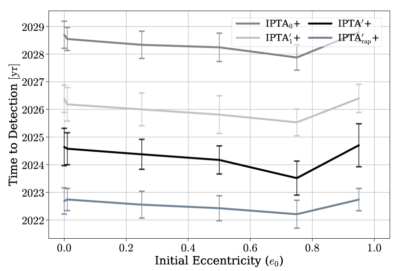
Figure 18: Time to detection versus initial eccentricity for the same four International PTA configurations discussed above. Differences in pulsar characteristics (most notably noise properties) and expansion prescriptions yield a 6 year range in times to detection.

References

- Amaro-Seoane et al. (2010) Amaro-Seoane P., Sesana A., Hoffman L., Benacquista M., Eichhorn C., Makino J., Spurzem R., 2010, Mon. Not. R. Astron. Soc., 402, 2308
- Amaro-Seoane et al. (2016) Amaro-Seoane P., Maureira-Fredes C., Dotti M., Colpi M., 2016, Astron. Astrophys., 591, A114
- Armitage & Natarajan (2005) Armitage P. J., Natarajan P., 2005, Astrophys. J., 634, 921
- Arzoumanian et al. (2015) Arzoumanian Z., et al., 2015, preprint, (arXiv:1508.03024)
- Astropy Collaboration et al. (2013) Astropy Collaboration et al., 2013, Astron. Astrophys., 558, A33
- Begelman et al. (1980) Begelman M. C., Blandford R. D., Rees M. J., 1980, Nature, 287, 307
- Binney & Tremaine (1987) Binney J., Tremaine S., 1987, Galactic dynamics. Princeton University Press
- Bonetti et al. (2016) Bonetti M., Haardt F., Sesana A., Barausse E., 2016, Mon. Not. R. Astron. Soc., 461, 4419
- Burke-Spolaor (2013) Burke-Spolaor S., 2013, Classical and Quantum Gravity, 30, 224013
- Caballero et al. (2016) Caballero R. N., et al., 2016, Mon. Not. R. Astron. Soc., 457, 4421
- Chandrasekhar (1943) Chandrasekhar S., 1943, Astrophys. J., 97, 255
- Chen et al. (2016) Chen S., Sesana A., Del Pozzo W., 2016, preprint, (arXiv:1612.00455)
- Chen et al. (2017) Chen S., Middleton H., Sesana A., Del Pozzo W., Vecchio A., 2017, Mon. Not. R. Astron. Soc., 468, 404
- Colpi et al. (1999) Colpi M., Mayer L., Governato F., 1999, Astrophys. J., 525, 720
- Cornish & Sampson (2016) Cornish N. J., Sampson L., 2016, Phys. Rev. D, 93, 104047
- Cuadra et al. (2009) Cuadra J., Armitage P. J., Alexander R. D., Begelman M. C., 2009, Mon. Not. R. Astron. Soc., 393, 1423
- Dehnen (1993) Dehnen W., 1993, Mon. Not. R. Astron. Soc., 265, 250
- Desvignes et al. (2016) Desvignes G., et al., 2016, Mon. Not. R. Astron. Soc., 458, 3341
- Detweiler (1979) Detweiler S., 1979, Astrophys. J., 234, 1100
- Enoki & Nagashima (2007) Enoki M., Nagashima M., 2007, Progress of Theoretical Physics, 117, 241
- Faber et al. (1997) Faber S. M., et al., 1997, Astron. J., 114, 1771
- Finn et al. (2009) Finn L. S., Larson S. L., Romano J. D., 2009, Phys. Rev. D, 79, 062003
- Foster & Backer (1990) Foster R. S., Backer D. C., 1990, Astrophys. J., 361, 300
- Genel et al. (2014) Genel S., et al., 2014, Mon. Not. R. Astron. Soc., 445, 175
- Haiman et al. (2009) Haiman Z., Kocsis B., Menou K., 2009, Astrophys. J., 700, 1952
- Hashimoto et al. (2003) Hashimoto Y., Funato Y., Makino J., 2003, Astrophys. J., 582, 196
- Hellings & Downs (1983) Hellings R. W., Downs G. S., 1983, Astrophys. J. Lett., 265, L39
- Hernquist (1990) Hernquist L., 1990, Astrophys. J., 356, 359
- Hobbs et al. (2010) Hobbs G., et al., 2010, Classical and Quantum Gravity, 27, 084013
- Hoffman & Loeb (2007) Hoffman L., Loeb A., 2007, Mon. Not. R. Astron. Soc., 377, 957
- Hogg (1999) Hogg D. W., 1999, ArXiv Astrophysics e-prints,
- Huerta et al. (2015) Huerta E. A., McWilliams S. T., Gair J. R., Taylor S. R., 2015, Phys. Rev. D, 92, 063010
- Hunter (2007) Hunter J. D., 2007, Computing In Science & Engineering, 9, 90
- Hut (1983) Hut P., 1983, Astrophys. J. Lett., 272, L29
- Jaffe & Backer (2003) Jaffe A. H., Backer D. C., 2003, The Astrophysical Journal, 583, 616
- Jones et al. (01 ) Jones E., Oliphant T., Peterson P., et al., 2001–, SciPy: Open source scientific tools for Python, http://www.scipy.org/
- Kelley et al. (2016) Kelley L. Z., Blecha L., Hernquist L., 2016, preprint, (arXiv:1606.01900)
- Khan et al. (2011) Khan F. M., Just A., Merritt D., 2011, Astrophys. J., 732, 89
- Kocsis & Sesana (2011) Kocsis B., Sesana A., 2011, Mon. Not. R. Astron. Soc., 411, 1467
- Kramer & Champion (2013) Kramer M., Champion D. J., 2013, Classical and Quantum Gravity, 30, 224009
- Lauer et al. (2007) Lauer T. R., et al., 2007, Astrophys. J., 664, 226
- Lentati et al. (2015) Lentati L., et al., 2015, Mon. Not. R. Astron. Soc., 453, 2576
- Lentati et al. (2016) Lentati L., et al., 2016, Mon. Not. R. Astron. Soc., 458, 2161
- Magorrian & Tremaine (1999) Magorrian J., Tremaine S., 1999, Mon. Not. R. Astron. Soc., 309, 447
- Manchester et al. (2013) Manchester R. N., et al., 2013, PASA, 30, e017
- McLaughlin (2013) McLaughlin M. A., 2013, Classical and Quantum Gravity, 30, 224008
- McWilliams et al. (2014) McWilliams S. T., Ostriker J. P., Pretorius F., 2014, Astrophys. J., 789, 156
- Milosavljević & Merritt (2003) Milosavljević M., Merritt D., 2003, Astrophys. J., 596, 860
- Moore et al. (2015) Moore C. J., Taylor S. R., Gair J. R., 2015, Classical and Quantum Gravity, 32, 055004
- Nelson et al. (2015) Nelson D., et al., 2015, Astronomy and Computing, 13, 12
- Peters (1964) Peters P. C., 1964, Physical Review, 136, 1224
- Peters & Mathews (1963) Peters P. C., Mathews J., 1963, Physical Review, 131, 435
- Phinney (2001) Phinney E. S., 2001, ArXiv Astrophysics e-prints,
- P rez & Granger (2007) P rez F., Granger B., 2007, Computing in Science Engineering, 9, 21
- Quinlan (1996) Quinlan G. D., 1996, New Astron., 1, 35
- Quinlan & Hernquist (1997) Quinlan G. D., Hernquist L., 1997, New Astron., 2, 533
- Rajagopal & Romani (1994) Rajagopal M., Romani R., 1994, arXiv preprint astro-ph/9412038
- Rajagopal & Romani (1995) Rajagopal M., Romani R. W., 1995, Astrophys. J., 446, 543
- Rantala et al. (2016) Rantala A., Pihajoki P., Johansson P. H., Naab T., Lahén N., Sawala T., 2016, preprint, (arXiv:1611.07028)
- Rasskazov & Merritt (2016) Rasskazov A., Merritt D., 2016, preprint, (arXiv:1606.07484)
- Ravi et al. (2012) Ravi V., Wyithe J. S. B., Hobbs G., Shannon R. M., Manchester R. N., Yardley D. R. B., Keith M. J., 2012, Astrophys. J., 761, 84
- Ravi et al. (2014) Ravi V., Wyithe J. S. B., Shannon R. M., Hobbs G., Manchester R. N., 2014, Mon. Not. R. Astron. Soc., 442, 56
- Reardon et al. (2016) Reardon D. J., et al., 2016, Mon. Not. R. Astron. Soc., 455, 1751
- Roebber et al. (2016) Roebber E., Holder G., Holz D. E., Warren M., 2016, Astrophys. J., 819, 163
- Roedig et al. (2011) Roedig C., Dotti M., Sesana A., Cuadra J., Colpi M., 2011, Mon. Not. R. Astron. Soc., 415, 3033
- Romani & Taylor (1983) Romani R. W., Taylor J. H., 1983, Astrophys. J. Lett., 265, L35
- Rosado et al. (2015) Rosado P. A., Sesana A., Gair J., 2015, Mon. Not. R. Astron. Soc., 451, 2417
- Sazhin (1978) Sazhin M. V., 1978, Soviet Astronomy, 22, 36
- Sesana (2010) Sesana A., 2010, Astrophys. J., 719, 851
- Sesana (2013) Sesana A., 2013, Mon. Not. R. Astron. Soc., 433, L1
- Sesana & Khan (2015) Sesana A., Khan F. M., 2015, Mon. Not. R. Astron. Soc., 454, L66
- Sesana et al. (2006) Sesana A., Haardt F., Madau P., 2006, Astrophys. J., 651, 392
- Sesana et al. (2008) Sesana A., Vecchio A., Colacino C. N., 2008, Mon. Not. R. Astron. Soc., 390, 192
- Sesana et al. (2011) Sesana A., Gualandris A., Dotti M., 2011, Mon. Not. R. Astron. Soc., 415, L35
- Sesana et al. (2012) Sesana A., Roedig C., Reynolds M. T., Dotti M., 2012, Mon. Not. R. Astron. Soc., 420, 860
- Sesana et al. (2016) Sesana A., Shankar F., Bernardi M., Sheth R. K., 2016, preprint, (arXiv:1603.09348)
- Shankar et al. (2016) Shankar F., et al., 2016, Mon. Not. R. Astron. Soc., 460, 3119
- Shannon et al. (2015) Shannon R. M., et al., 2015, Science, 349, 1522
- Shapiro & Teukolsky (1986) Shapiro S. L., Teukolsky S. A., 1986, Black Holes, White Dwarfs and Neutron Stars: The Physics of Compact Objects
- Shen et al. (2008) Shen Y., Greene J. E., Strauss M. A., Richards G. T., Schneider D. P., 2008, Astrophys. J., 680, 169
- Sijacki et al. (2015) Sijacki D., Vogelsberger M., Genel S., Springel V., Torrey P., Snyder G. F., Nelson D., Hernquist L., 2015, Mon. Not. R. Astron. Soc., 452, 575
- Snyder et al. (2015) Snyder G. F., et al., 2015, Mon. Not. R. Astron. Soc., 454, 1886
- Springel (2010) Springel V., 2010, Mon. Not. R. Astron. Soc., 401, 791
- Tanaka et al. (2012) Tanaka T., Menou K., Haiman Z., 2012, Mon. Not. R. Astron. Soc., 420, 705
- Taylor et al. (2016) Taylor S. R., Vallisneri M., Ellis J. A., Mingarelli C. M. F., Lazio T. J. W., van Haasteren R., 2016, Astrophys. J. Lett., 819, L6
- Taylor et al. (2017) Taylor S. R., Simon J., Sampson L., 2017, Physical Review Letters, 118, 181102
- The NANOGrav Collaboration et al. (2015) The NANOGrav Collaboration et al., 2015, Astrophys. J., 813, 65
- Torrey et al. (2014) Torrey P., Vogelsberger M., Genel S., Sijacki D., Springel V., Hernquist L., 2014, Mon. Not. R. Astron. Soc., 438, 1985
- Van Der Walt et al. (2011) Van Der Walt S., Colbert S. C., Varoquaux G., 2011, preprint, (arXiv:1102.1523)
- Vasiliev et al. (2015) Vasiliev E., Antonini F., Merritt D., 2015, Astrophys. J., 810, 49
- Verbiest et al. (2016) Verbiest J. P. W., et al., 2016, preprint, (arXiv:1602.03640)
- Vigeland & Siemens (2016) Vigeland S. J., Siemens X., 2016, Phys. Rev. D, 94, 123003
- Vogelsberger et al. (2013) Vogelsberger M., Genel S., Sijacki D., Torrey P., Springel V., Hernquist L., 2013, Mon. Not. R. Astron. Soc., 436, 3031
- Vogelsberger et al. (2014a) Vogelsberger M., et al., 2014a, Mon. Not. R. Astron. Soc., 444, 1518
- Vogelsberger et al. (2014b) Vogelsberger M., et al., 2014b, Nature, 509, 177
- Volonteri et al. (2003) Volonteri M., Madau P., Haardt F., 2003, Astrophys. J., 593, 661
- Wyithe & Loeb (2003) Wyithe J. S. B., Loeb A., 2003, Astrophys. J., 590, 691
- de Vaucouleurs (1948) de Vaucouleurs G., 1948, Annales d’Astrophysique, 11, 247
- van den Bosch et al. (1999) van den Bosch F. C., Lewis G. F., Lake G., Stadel J., 1999, Astrophys. J., 515, 50