PHYSICAL REVIEW D 96 (2017) 103511

Echo of interactions in the dark sector

Abstract

We investigate the observational constraints on an interacting vacuum energy scenario with two different neutrino schemes (with and without a sterile neutrino) using the most recent data from CMB temperature and polarization anisotropy, baryon acoustic oscillations (BAO), type Ia supernovae from JLA sample and structure growth inferred from cluster counts. We find that inclusion of the galaxy clusters data with the minimal data combination CMB + BAO + JLA suggests an interaction in the dark sector, implying the decay of dark matter particles into dark energy, since the constraints obtained by including the galaxy clusters data yield a non-null and negative coupling parameter between the dark components at 99% confidence level. We deduce that the current tensions on the parameters $H_{0}$ and $\sigma_{8}$ can be alleviated within the framework of the interacting as well as non-interacting vacuum energy models with sterile neutrinos.

I Introduction

Since the discovery that our Universe is in a current stage of accelerated expansion int1 ; int2 , the inclusion of an exotic energy component with negative pressure, dubbed as dark energy (DE), in the energy budget of the Universe is necessary to explain the observations. A cosmological model with cold dark matter (CDM) and DE mimicked by a positive cosmological constant $\Lambda$, the so-called $\Lambda$CDM model, is considered as the standard cosmological model for its ability to fit the observational data with great precision. A large amount of data, pouring in from different physical origins, have been measured with good precision to unveil the dynamics/mysteries of the Universe in the last decade or so. Some data sets are found in tension with others within the framework of the $\Lambda$CDM model (seeT1 ; T2 ; T3 ; T4 ; T5 ), which could be an indication of new physics beyond $\Lambda$CDM model or may be due to some systematic effects on the data. Also, the cosmological constant suffers from some theoretical problems int3 ; int4a ; int4b ; int5 , which motivated the researchers to propose new models of DE, or alternative mechanisms that can explain the observational data without the need for DE, such as modified gravity models. Cosmological models, where dark matter (DM) and DE interact throughout the evolution history of the Universe, have received considerable attention of the researchers in the recent past in order to solve/assuage the problem of the cosmic coincidence as well as the problem of the cosmological constant (for the case where DM interacts with vacuum energy). See DE_DM_1 ; DE_DM_2 for general review. The late-time interaction in the dark sector has recently been investigated in various studies Salvatelli ; Sola1 ; Sola2 ; Saulo ; Richarte ; Valiviita ; Elisa ; Murgia:2016ccp ; N1 ; N2 ; N3 ; N4 ; N5 in different contexts.

On the other hand, physical experiments from solar, atmospheric, reactor and accelerator neutrino beams have proved the existence of neutrino oscillations (see Garcia and references therein for review and Garcia2 ; Capozzi for current experimental status). The phenomenon of neutrino oscillations implies directly a non-zero neutrino mass, once the neutrino oscillations depend only on the mass difference between the three species predicted by the standard model of particle physics. Non-standard neutrinos, like the sterile massive neutrinos, are predicted in a natural extension of the standard model of elementary particles. Sterile neutrinos at the eV mass scale, can explain the anomalies found in some short-baseline neutrino oscillation experiments from the reactor antineutrino anomaly, the Gallium neutrino anomaly, and LSND experiments (see Palazzo ; Abazajian ; Gariazzo for review). These experiments require the existence of light sterile neutrinos.

Massive neutrinos play an important role on cosmological scales, with direct implications on Cosmic Microwave Background (CMB) temperature and polarization anisotropy, large scale structure, nuclear abundances produced by big bang nucleosynthesis, and in some other cosmological sources (see Dolgov ; Lesgourgues ; Lesgourgues2 for review, Planck collaboration paper Planck2015 , and forecast from CORE space mission CORE for observational constraints). Recently, cosmological models with massive neutrinos have been studied to reconcile the tension between local and global determinations of the Hubble constant Valentino ; Bernal ; Wyman ; Riess ; Tram . The presence of massive neutrinos in cosmological models is useful to investigate the accuracy and robustness of a given scenario. The cosmological effects of light sterile neutrinos are investigated in different contexts m_esteril1 ; m_esteril2 ; m_esteril3 ; m_esteril4 ; m_esteril5 ; m_esteril6

In this paper, we are motivated to investigate a coupled DE scenario, where vacuum energy interacts with DM, by considering neutrinos scheme with sum of the active neutrino masses ($\sum m_{\nu}$) and the effective number of relativistic degrees of freedom ($N_{\rm eff}$) as free quantities. In addition, we consider the models with one non-standard neutrino (sterile neutrino) beyond the three species predicted by the standard model, the so-called (3 + 1) models. We study observational constraints on the models by using the most recent data from CMB temperature and polarization anisotropy, baryon acoustic oscillations, type Ia supernovae from JLA sample, and galaxy clusters measurements. Our main result is that the coupling parameter of the dark sector is observed to be non-zero up to $99\%$ confidence level (CL).

Rest of the paper is structured as follows: The interacting vacuum energy scenario is introduced in the following Section II while different models of neutrinos with the interacting as well as non-interacting vacuum energy scenario are described in Section III. The observational constraints from various recent data sets on the models under consideration are obtained and discussed in detail in Section IV. The conclusions the our investigation are summarized in the final section.

II Interaction in the dark sector

We consider a spatially-flat Friedmann-Robertson-Walker Universe, with the Friedmann equation given by

$$3H^{2}=8\pi G(\rho_{\gamma}+\rho_{\nu}+\rho_{\rm b}+\rho_{\rm dm}+\rho_{\rm de}),$$ (1)

where $H=\dot{a}/a$ is the Hubble parameter. Further $\rho_{\gamma}$, $\rho_{\nu}$, $\rho_{\rm b}$, $\rho_{\rm dm}$, and $\rho_{\rm de}$ stand for the energy densities of photons, massive neutrinos, baryons, cold DM and DE, respectively.

We assume that DM and DE interact via the coupling function $Q$ given by

$$\dot{\rho}_{\rm dm}+3H\rho_{\rm dm}=-\dot{\rho}_{\rm de}-3H\rho_{\rm de}(1+w_{\rm de})=Q.$$ (2)

For $Q>0$, the energy flow takes place from DE to DM, otherwise the energy flows from DM to DE. The parameter $w_{\rm de}$ is the equation of state of the DE and in general can be constant or variable. In order to avoid many free parameters, we consider the simplest case $w_{\rm de}=-1$, i.e., an interacting vacuum energy scenario. In what follows, we refer this model to as IVCDM model. For the sake of comparison, we shall also consider the non-interacting vacuum energy case ($\delta=0$), i.e., the $\Lambda$CDM model.

Recent studies of interacting vacuum cosmologies have focused on models with general interaction term given by $Q=\delta H\rho_{\rm dm}$ or $Q=\delta H\rho_{\rm de}$, where $\delta$ is a constant and dimensionless parameter that characterizes the interaction between DM and DE. Both classes have been investigated from different perspectives coupled01 ; coupled02 ; coupled03 ; coupled04 ; coupled05 ; coupled06 ; coupled07 ; coupled08 ; coupled09 ; coupled10 ; coupled11 ; coupled12 . For instance, indelta_cdm3 , we investigated the interaction in dark sector given by the coupling function $Q=\delta H\rho_{\rm dm}$. We noted that this coupling function may suffer from instability in the dark sector perturbations at early times (the curvature perturbations may blow up on super Hubble scales), and to avoid such problems we should have $\delta<10^{-2}$. On the other hand, it is known that $Q=\delta H\rho_{\rm de}$ does not present these problems delta_cdm4 , and that the coupling parameter $\delta$ can admit much larger values. Once we consider data from perturbative origin in our analysis, the choice $Q=\delta H\rho_{\rm de}$ offers a greater range of security/freedom over the coupling parameter, and thus allows this parameter to be constrained within a larger prior range. For instance, the authors in Salvatelli used this coupling function to show that a general late-time interaction between cold DM and vacuum energy is favored by current cosmological datasets. Therefore, in the present study, we use the coupling function given by $Q=\delta H\rho_{\rm de}$. Once the coupling function $Q$ has been defined, the background evolution of the dark components can be obtained from eq. (2). Here, we adopt the synchronous gauge for the evolution of the scalar mode perturbations of the dark components as in delta_cdm ; delta_cdm2 , or more explicitly the eqs. (6) - (9) of delta_cdm3 . The baryons, photons and massive neutrinos are conserved independently, and the perturbation equations follow the standard evolution as described in Ma_Bertschinger .

III The models

On the basis of neutrinos, we consider the following models in our study.

$\checkmark$ We consider the interacting and non-interacting vacuum energy scenarios possessing neutrinos scheme with sum of the active neutrino masses ($\sum m_{\nu}$) and the effective number of relativistic degrees of freedom ($N_{\rm eff}$) as free quantities. In our results, we shall denote these models as $\nu$IVCDM and $\nu\Lambda$CDM, respectively.

$\checkmark$ Following the Planck collaboration, we fix the mass ordering of the active neutrinos to the normal hierarchy with the minimum masses allowed by oscillation experiments, i.e., $\sum m_{\nu}=0.06$ eV. As generalization, let us take the mass order, $m_{1}=m_{2}=0$ eV and $m_{3}=0.06$ eV. Therefore, the presence of excess mass can be considered from a single additional mass state $m_{4}$, which can be related to the sterile neutrino mass, $m_{{\nu}_{s}}$. Taking this into account, the mass splitting with relation to the sterile neutrino can be written as $\Delta m_{41}=m_{4}$. In order to constrain the sterile neutrino mass, the effective number of neutrino species is $N_{\rm eff}=4.046$, i.e., we consider one species of sterile neutrinos (fully thermalized) beyond the three neutrino species of the standard model, the so-called (3+1) models. We consider the sterile neutrino case with the interacting and non-interacting vacuum energy scenarios, and denote these models as $\nu_{s}$IVCDM and $\nu_{s}\Lambda$CDM, respectively.

IV Observational Constraints

In order to constrain the models under consideration, we use the following data sets.

CMB: The cosmic microwave background (CMB) data from Planck 2015 comprised of the likelihoods at multipoles $l\geq 30$ using TT, TE and EE power spectra and the low-multipole polarization likelihood at $l\leq 29$. The combination of these data is referred to as Planck TT, TE, EE + lowP in Planck2015 . We also include Planck 2015 CMB lensing power spectrum likelihood CMB .

BAO: The baryon acoustic oscillations (BAO) measurements from the Six Degree Field Galaxy Survey (6dF) bao1 , the Main Galaxy Sample of Data Release 7 of Sloan Digital Sky Survey (SDSS-MGS) bao2 , the LOWZ and CMASS galaxy samples of the Baryon Oscillation Spectroscopic Survey (BOSS-LOWZ and BOSS-CMASS, respectively) bao3 , and the distribution of the LymanForest in BOSS (BOSS-Ly) bao4 . These data points are summarized in table I of coupled04 .

JLA: The latest “joint light curves” (JLA) sample snia3 , comprised of 740 type Ia supernovae in the redshift range $z\in[0.01,1.30]$.

GC: The measurements from the abundance of galaxy clusters (GC) offer a powerful probe of the growth of cosmic structures. The cosmological information enclosed in the cluster abundance is efficiently parameterized by $S_{8}=\sigma_{8}(\Omega_{m}/\alpha)^{\beta}$, where $\sigma_{8}$ is the linear amplitude of the fluctuations on 8 Mpc/h scale and $\alpha$, $\beta$ are adopted/fit parameters in each survey analysis. We use the measurements from the Sunyaev-Zeldovich effect cluster mass function measured by Planck (SZ) cg1 ($\alpha=0.27$ and $\beta=0.30$) and the constraints derived by weak gravitational lensing data from Canada-France-Hawaii Telescope Lensing Survey (CFHTLenS) cg2 ($\alpha=0.27$ and $\beta=0.46$).

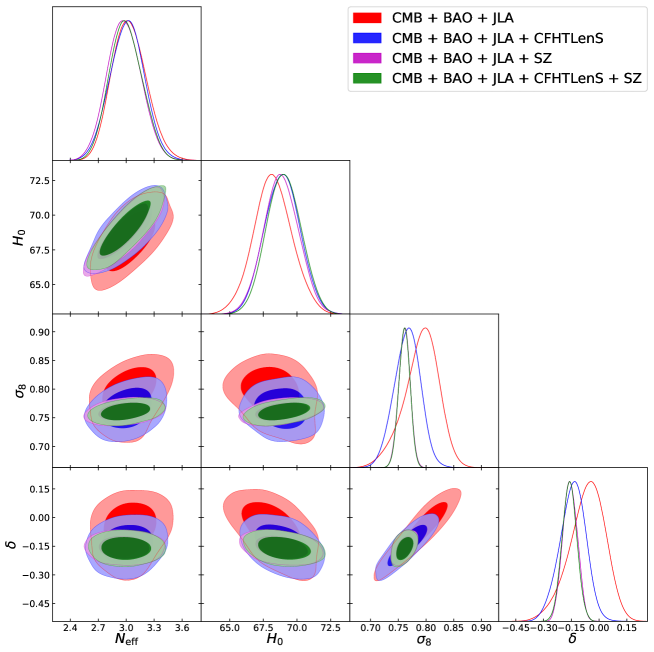
We modified the publicly available CLASS class and Monte Python monte codes for the models considered in the present work. We used Metropolis Hastings algorithm with uniform priors on the model parameters to obtain correlated Markov Chain Monte Carlo samples by considering four combinations of data sets: CMB + BAO + JLA, CMB + BAO + JLA + CFHTLenS, CMB + BAO + JLA + SZ, and CMB + BAO + JLA + CFHTLenS + SZ. All parameters in our Monte Carlo Markov Chains converge according to the Gelman-Rubin criteria Gelman . The resulting samples are then analysed by using the GetDist Python package antonygetdist . Note that we have chosen the minimal data set CMB+BAO+JLA because adding BAO + JLA data to CMB does not shift the regions of probability much, but this combination constrains the matter density very well, and reduces the error-bars on the parameters. The other data set combinations are considered to investigate how the constraints on various free parameters and derived parameters are affected by the inclusion of GC data. The final statistical results are summarized in Table 1.

Figure 1: One-dimensional marginalized distribution, and 68% and 95% CL regions for some selected parameters of the $\nu$IVCDM model.

Figure 2: One-dimensional marginalized distribution, and 68% and 95% CL regions for some selected parameters of the $\nu_{s}$IVCDM model.

Table 1: Constraints on free parameters and two derived parameters $H_{0}$ and $\sigma_{8}$ of the $\nu$IVCDM, $\nu\Lambda$CDM, $\nu_{s}$IVCDM and $\nu_{s}\Lambda$CDM models. For each parameter, the four entries (mean values with 1$\sigma$ errors) are the constraints from the data combinations CMB + BAO + JLA, CMB + BAO + JLA + CFHTLenS, CMB + BAO + JLA + SZ and CMB + BAO + JLA + CFHTLenS + SZ, respectively. The parameter $H_{0}$ is in the units of km s^-1 Mpc^-1, while $\sum m_{\nu}$ and $m_{{\nu}_{s}}$ are in the units of eV. The $\chi^{2}_{\rm min}$ values of the fit are also displayed.

	$\nu$IVCDM	$\nu\Lambda$CDM	$\nu_{s}$IVCDM	$\nu_{s}\Lambda$CDM
$10^{2}\omega_{\rm b}$	${\color[rgb]{1,0,0}\definecolor[named]{pgfstrokecolor}{rgb}{1,0,0}2.230\pm 0.021}$	${\color[rgb]{1,0,0}\definecolor[named]{pgfstrokecolor}{rgb}{1,0,0}2.238\pm 0.019}$	${\color[rgb]{1,0,0}\definecolor[named]{pgfstrokecolor}{rgb}{1,0,0}2.314\pm 0.014}$	${\color[rgb]{1,0,0}\definecolor[named]{pgfstrokecolor}{rgb}{1,0,0}2.311\pm 0.016}$
	${\color[rgb]{0,0,1}\definecolor[named]{pgfstrokecolor}{rgb}{0,0,1}2.226\pm 0.021}$	${\color[rgb]{0,0,1}\definecolor[named]{pgfstrokecolor}{rgb}{0,0,1}2.241\pm 0.020}$	${\color[rgb]{0,0,1}\definecolor[named]{pgfstrokecolor}{rgb}{0,0,1}2.308\pm 0.015}$	${\color[rgb]{0,0,1}\definecolor[named]{pgfstrokecolor}{rgb}{0,0,1}2.314\pm 0.015}$
	${\color[rgb]{1,0,1}\definecolor[named]{pgfstrokecolor}{rgb}{1,0,1}\pgfsys@color@cmyk@stroke{0}{1}{0}{0}\pgfsys@color@cmyk@fill{0}{1}{0}{0}2.222\pm 0.020}$	${\color[rgb]{1,0,1}\definecolor[named]{pgfstrokecolor}{rgb}{1,0,1}\pgfsys@color@cmyk@stroke{0}{1}{0}{0}\pgfsys@color@cmyk@fill{0}{1}{0}{0}2.241\pm 0.022}$	${\color[rgb]{1,0,1}\definecolor[named]{pgfstrokecolor}{rgb}{1,0,1}\pgfsys@color@cmyk@stroke{0}{1}{0}{0}\pgfsys@color@cmyk@fill{0}{1}{0}{0}2.308\pm 0.014}$	${\color[rgb]{1,0,1}\definecolor[named]{pgfstrokecolor}{rgb}{1,0,1}\pgfsys@color@cmyk@stroke{0}{1}{0}{0}\pgfsys@color@cmyk@fill{0}{1}{0}{0}2.323\pm 0.014}$
	${\color[rgb]{0.,0.65,0.1}\definecolor[named]{pgfstrokecolor}{rgb}{0.,0.65,0.1}2.224\pm 0.020}$	${\color[rgb]{0.,0.65,0.1}\definecolor[named]{pgfstrokecolor}{rgb}{0.,0.65,0.1}2.241\pm 0.021}$	${\color[rgb]{0.,0.65,0.1}\definecolor[named]{pgfstrokecolor}{rgb}{0.,0.65,0.1}2.307\pm 0.015}$	${\color[rgb]{0.,0.65,0.1}\definecolor[named]{pgfstrokecolor}{rgb}{0.,0.65,0.1}2.326\pm 0.015}$
$\omega_{\rm{cdm}}$	${\color[rgb]{1,0,0}\definecolor[named]{pgfstrokecolor}{rgb}{1,0,0}0.1182\pm 0.0028}$	${\color[rgb]{1,0,0}\definecolor[named]{pgfstrokecolor}{rgb}{1,0,0}0.1188^{+0.0028}_{-0.0031}}$	${\color[rgb]{1,0,0}\definecolor[named]{pgfstrokecolor}{rgb}{1,0,0}0.1322\pm 0.0013}$	${\color[rgb]{1,0,0}\definecolor[named]{pgfstrokecolor}{rgb}{1,0,0}0.1326\pm 0.0015}$
	${\color[rgb]{0,0,1}\definecolor[named]{pgfstrokecolor}{rgb}{0,0,1}0.1182\pm 0.0029}$	${\color[rgb]{0,0,1}\definecolor[named]{pgfstrokecolor}{rgb}{0,0,1}0.1181\pm 0.0029}$	${\color[rgb]{0,0,1}\definecolor[named]{pgfstrokecolor}{rgb}{0,0,1}0.1325\pm 0.0015}$	${\color[rgb]{0,0,1}\definecolor[named]{pgfstrokecolor}{rgb}{0,0,1}0.1318\pm 0.0014}$
	${\color[rgb]{1,0,1}\definecolor[named]{pgfstrokecolor}{rgb}{1,0,1}\pgfsys@color@cmyk@stroke{0}{1}{0}{0}\pgfsys@color@cmyk@fill{0}{1}{0}{0}0.1178\pm 0.0029}$	${\color[rgb]{1,0,1}\definecolor[named]{pgfstrokecolor}{rgb}{1,0,1}\pgfsys@color@cmyk@stroke{0}{1}{0}{0}\pgfsys@color@cmyk@fill{0}{1}{0}{0}0.1152\pm 0.0029}$	${\color[rgb]{1,0,1}\definecolor[named]{pgfstrokecolor}{rgb}{1,0,1}\pgfsys@color@cmyk@stroke{0}{1}{0}{0}\pgfsys@color@cmyk@fill{0}{1}{0}{0}0.1324\pm 0.0015}$	${\color[rgb]{1,0,1}\definecolor[named]{pgfstrokecolor}{rgb}{1,0,1}\pgfsys@color@cmyk@stroke{0}{1}{0}{0}\pgfsys@color@cmyk@fill{0}{1}{0}{0}0.1293\pm 0.0012}$
	${\color[rgb]{0.,0.65,0.1}\definecolor[named]{pgfstrokecolor}{rgb}{0.,0.65,0.1}0.1181\pm 0.0028}$	${\color[rgb]{0.,0.65,0.1}\definecolor[named]{pgfstrokecolor}{rgb}{0.,0.65,0.1}0.1149\pm 0.0030}$	${\color[rgb]{0.,0.65,0.1}\definecolor[named]{pgfstrokecolor}{rgb}{0.,0.65,0.1}0.1325\pm 0.0015}$	${\color[rgb]{0.,0.65,0.1}\definecolor[named]{pgfstrokecolor}{rgb}{0.,0.65,0.1}0.1290\pm 0.0011}$
$100\theta_{s}$	${\color[rgb]{1,0,0}\definecolor[named]{pgfstrokecolor}{rgb}{1,0,0}1.04200\pm 0.00049}$	${\color[rgb]{1,0,0}\definecolor[named]{pgfstrokecolor}{rgb}{1,0,0}1.04185\pm 0.00049}$	${\color[rgb]{1,0,0}\definecolor[named]{pgfstrokecolor}{rgb}{1,0,0}1.04005\pm 0.00029}$	${\color[rgb]{1,0,0}\definecolor[named]{pgfstrokecolor}{rgb}{1,0,0}1.04000\pm 0.00030}$
	${\color[rgb]{0,0,1}\definecolor[named]{pgfstrokecolor}{rgb}{0,0,1}1.04200\pm 0.00051}$	${\color[rgb]{0,0,1}\definecolor[named]{pgfstrokecolor}{rgb}{0,0,1}1.04190\pm 0.00048}$	${\color[rgb]{0,0,1}\definecolor[named]{pgfstrokecolor}{rgb}{0,0,1}1.04005\pm 0.00029}$	${\color[rgb]{0,0,1}\definecolor[named]{pgfstrokecolor}{rgb}{0,0,1}1.04007\pm 0.00030}$
	${\color[rgb]{1,0,1}\definecolor[named]{pgfstrokecolor}{rgb}{1,0,1}\pgfsys@color@cmyk@stroke{0}{1}{0}{0}\pgfsys@color@cmyk@fill{0}{1}{0}{0}1.04026\pm 0.00030}$	${\color[rgb]{1,0,1}\definecolor[named]{pgfstrokecolor}{rgb}{1,0,1}\pgfsys@color@cmyk@stroke{0}{1}{0}{0}\pgfsys@color@cmyk@fill{0}{1}{0}{0}1.04219\pm 0.00053}$	${\color[rgb]{1,0,1}\definecolor[named]{pgfstrokecolor}{rgb}{1,0,1}\pgfsys@color@cmyk@stroke{0}{1}{0}{0}\pgfsys@color@cmyk@fill{0}{1}{0}{0}1.04002\pm 0.00029}$	${\color[rgb]{1,0,1}\definecolor[named]{pgfstrokecolor}{rgb}{1,0,1}\pgfsys@color@cmyk@stroke{0}{1}{0}{0}\pgfsys@color@cmyk@fill{0}{1}{0}{0}1.04032\pm 0.00028}$
	${\color[rgb]{0.,0.65,0.1}\definecolor[named]{pgfstrokecolor}{rgb}{0.,0.65,0.1}1.04200\pm 0.00049}$	${\color[rgb]{0.,0.65,0.1}\definecolor[named]{pgfstrokecolor}{rgb}{0.,0.65,0.1}1.04221\pm 0.00053}$	${\color[rgb]{0.,0.65,0.1}\definecolor[named]{pgfstrokecolor}{rgb}{0.,0.65,0.1}1.04002\pm 0.00032}$	${\color[rgb]{0.,0.65,0.1}\definecolor[named]{pgfstrokecolor}{rgb}{0.,0.65,0.1}1.04032\pm 0.00028}$
$\ln 10^{10}A_{s}$	${\color[rgb]{1,0,0}\definecolor[named]{pgfstrokecolor}{rgb}{1,0,0}3.091^{+0.027}_{-0.030}}$	${\color[rgb]{1,0,0}\definecolor[named]{pgfstrokecolor}{rgb}{1,0,0}3.091\pm 0.026}$	${\color[rgb]{1,0,0}\definecolor[named]{pgfstrokecolor}{rgb}{1,0,0}3.149\pm 0.029}$	${\color[rgb]{1,0,0}\definecolor[named]{pgfstrokecolor}{rgb}{1,0,0}3.158\pm 0.032}$
	${\color[rgb]{0,0,1}\definecolor[named]{pgfstrokecolor}{rgb}{0,0,1}3.091\pm 0.028}$	${\color[rgb]{0,0,1}\definecolor[named]{pgfstrokecolor}{rgb}{0,0,1}3.086\pm 0.028}$	${\color[rgb]{0,0,1}\definecolor[named]{pgfstrokecolor}{rgb}{0,0,1}3.171\pm 0.031}$	${\color[rgb]{0,0,1}\definecolor[named]{pgfstrokecolor}{rgb}{0,0,1}3.164\pm 0.031}$
	${\color[rgb]{1,0,1}\definecolor[named]{pgfstrokecolor}{rgb}{1,0,1}\pgfsys@color@cmyk@stroke{0}{1}{0}{0}\pgfsys@color@cmyk@fill{0}{1}{0}{0}3.089^{+0.027}_{-0.031}}$	${\color[rgb]{1,0,1}\definecolor[named]{pgfstrokecolor}{rgb}{1,0,1}\pgfsys@color@cmyk@stroke{0}{1}{0}{0}\pgfsys@color@cmyk@fill{0}{1}{0}{0}3.079^{+0.033}_{-0.039}}$	${\color[rgb]{1,0,1}\definecolor[named]{pgfstrokecolor}{rgb}{1,0,1}\pgfsys@color@cmyk@stroke{0}{1}{0}{0}\pgfsys@color@cmyk@fill{0}{1}{0}{0}3.184\pm 0.029}$	${\color[rgb]{1,0,1}\definecolor[named]{pgfstrokecolor}{rgb}{1,0,1}\pgfsys@color@cmyk@stroke{0}{1}{0}{0}\pgfsys@color@cmyk@fill{0}{1}{0}{0}3.190\pm 0.029}$
	${\color[rgb]{0.,0.65,0.1}\definecolor[named]{pgfstrokecolor}{rgb}{0.,0.65,0.1}3.089^{+0.025}_{-0.030}}$	${\color[rgb]{0.,0.65,0.1}\definecolor[named]{pgfstrokecolor}{rgb}{0.,0.65,0.1}3.076^{+0.034}_{-0.038}}$	${\color[rgb]{0.,0.65,0.1}\definecolor[named]{pgfstrokecolor}{rgb}{0.,0.65,0.1}3.186\pm 0.028}$	${\color[rgb]{0.,0.65,0.1}\definecolor[named]{pgfstrokecolor}{rgb}{0.,0.65,0.1}3.193\pm 0.028}$
$n_{s}$	${\color[rgb]{1,0,0}\definecolor[named]{pgfstrokecolor}{rgb}{1,0,0}0.9667\pm 0.0082}$	${\color[rgb]{1,0,0}\definecolor[named]{pgfstrokecolor}{rgb}{1,0,0}0.9703\pm 0.0080}$	${\color[rgb]{1,0,0}\definecolor[named]{pgfstrokecolor}{rgb}{1,0,0}1.0050\pm 0.0043}$	${\color[rgb]{1,0,0}\definecolor[named]{pgfstrokecolor}{rgb}{1,0,0}1.0040\pm 0.0043}$
	${\color[rgb]{0,0,1}\definecolor[named]{pgfstrokecolor}{rgb}{0,0,1}0.9648\pm 0.0080}$	${\color[rgb]{0,0,1}\definecolor[named]{pgfstrokecolor}{rgb}{0,0,1}0.9703\pm 0.0076}$	${\color[rgb]{0,0,1}\definecolor[named]{pgfstrokecolor}{rgb}{0,0,1}1.0031\pm 0.0045}$	${\color[rgb]{0,0,1}\definecolor[named]{pgfstrokecolor}{rgb}{0,0,1}1.0049\pm 0.0043}$
	${\color[rgb]{1,0,1}\definecolor[named]{pgfstrokecolor}{rgb}{1,0,1}\pgfsys@color@cmyk@stroke{0}{1}{0}{0}\pgfsys@color@cmyk@fill{0}{1}{0}{0}0.9632\pm 0.0078}$	${\color[rgb]{1,0,1}\definecolor[named]{pgfstrokecolor}{rgb}{1,0,1}\pgfsys@color@cmyk@stroke{0}{1}{0}{0}\pgfsys@color@cmyk@fill{0}{1}{0}{0}0.9684\pm 0.0090}$	${\color[rgb]{1,0,1}\definecolor[named]{pgfstrokecolor}{rgb}{1,0,1}\pgfsys@color@cmyk@stroke{0}{1}{0}{0}\pgfsys@color@cmyk@fill{0}{1}{0}{0}1.0023\pm 0.0043}$	${\color[rgb]{1,0,1}\definecolor[named]{pgfstrokecolor}{rgb}{1,0,1}\pgfsys@color@cmyk@stroke{0}{1}{0}{0}\pgfsys@color@cmyk@fill{0}{1}{0}{0}1.0061\pm 0.0041}$
	${\color[rgb]{0.,0.65,0.1}\definecolor[named]{pgfstrokecolor}{rgb}{0.,0.65,0.1}0.9640\pm 0.0074}$	${\color[rgb]{0.,0.65,0.1}\definecolor[named]{pgfstrokecolor}{rgb}{0.,0.65,0.1}0.9680\pm 0.0087}$	${\color[rgb]{0.,0.65,0.1}\definecolor[named]{pgfstrokecolor}{rgb}{0.,0.65,0.1}1.0021\pm 0.0043}$	${\color[rgb]{0.,0.65,0.1}\definecolor[named]{pgfstrokecolor}{rgb}{0.,0.65,0.1}1.0070\pm 0.0041}$
$\tau_{\rm reio}$	${\color[rgb]{1,0,0}\definecolor[named]{pgfstrokecolor}{rgb}{1,0,0}0.080\pm 0.014}$	${\color[rgb]{1,0,0}\definecolor[named]{pgfstrokecolor}{rgb}{1,0,0}0.079\pm 0.013}$	${\color[rgb]{1,0,0}\definecolor[named]{pgfstrokecolor}{rgb}{1,0,0}0.094\pm 0.016}$	${\color[rgb]{1,0,0}\definecolor[named]{pgfstrokecolor}{rgb}{1,0,0}0.098\pm 0.017}$
	${\color[rgb]{0,0,1}\definecolor[named]{pgfstrokecolor}{rgb}{0,0,1}0.081\pm 0.014}$	${\color[rgb]{0,0,1}\definecolor[named]{pgfstrokecolor}{rgb}{0,0,1}0.078\pm 0.014}$	${\color[rgb]{0,0,1}\definecolor[named]{pgfstrokecolor}{rgb}{0,0,1}0.105\pm 0.017}$	${\color[rgb]{0,0,1}\definecolor[named]{pgfstrokecolor}{rgb}{0,0,1}0.102\pm 0.017}$
	${\color[rgb]{1,0,1}\definecolor[named]{pgfstrokecolor}{rgb}{1,0,1}\pgfsys@color@cmyk@stroke{0}{1}{0}{0}\pgfsys@color@cmyk@fill{0}{1}{0}{0}0.080\pm 0.014}$	${\color[rgb]{1,0,1}\definecolor[named]{pgfstrokecolor}{rgb}{1,0,1}\pgfsys@color@cmyk@stroke{0}{1}{0}{0}\pgfsys@color@cmyk@fill{0}{1}{0}{0}0.078^{+0.016}_{-0.018}}$	${\color[rgb]{1,0,1}\definecolor[named]{pgfstrokecolor}{rgb}{1,0,1}\pgfsys@color@cmyk@stroke{0}{1}{0}{0}\pgfsys@color@cmyk@fill{0}{1}{0}{0}0.113\pm 0.015}$	${\color[rgb]{1,0,1}\definecolor[named]{pgfstrokecolor}{rgb}{1,0,1}\pgfsys@color@cmyk@stroke{0}{1}{0}{0}\pgfsys@color@cmyk@fill{0}{1}{0}{0}0.118\pm 0.016}$
	${\color[rgb]{0.,0.65,0.1}\definecolor[named]{pgfstrokecolor}{rgb}{0.,0.65,0.1}0.079^{+0.013}_{-0.015}}$	${\color[rgb]{0.,0.65,0.1}\definecolor[named]{pgfstrokecolor}{rgb}{0.,0.65,0.1}0.077^{+0.016}_{-0.018}}$	${\color[rgb]{0.,0.65,0.1}\definecolor[named]{pgfstrokecolor}{rgb}{0.,0.65,0.1}0.113\pm 0.015}$	${\color[rgb]{0.,0.65,0.1}\definecolor[named]{pgfstrokecolor}{rgb}{0.,0.65,0.1}0.120\pm 0.015}$
$N_{\rm eff}$	${\color[rgb]{1,0,0}\definecolor[named]{pgfstrokecolor}{rgb}{1,0,0}3.03^{+0.17}_{-0.20}}$	${\color[rgb]{1,0,0}\definecolor[named]{pgfstrokecolor}{rgb}{1,0,0}3.10\pm 0.19}$	${\color[rgb]{1,0,0}\definecolor[named]{pgfstrokecolor}{rgb}{1,0,0}4.046}$	${\color[rgb]{1,0,0}\definecolor[named]{pgfstrokecolor}{rgb}{1,0,0}4.046}$
	${\color[rgb]{0,0,1}\definecolor[named]{pgfstrokecolor}{rgb}{0,0,1}3.01\pm 0.18}$	${\color[rgb]{0,0,1}\definecolor[named]{pgfstrokecolor}{rgb}{0,0,1}3.08\pm 0.18}$	${\color[rgb]{0,0,1}\definecolor[named]{pgfstrokecolor}{rgb}{0,0,1}4.046}$	${\color[rgb]{0,0,1}\definecolor[named]{pgfstrokecolor}{rgb}{0,0,1}4.046}$
	${\color[rgb]{1,0,1}\definecolor[named]{pgfstrokecolor}{rgb}{1,0,1}\pgfsys@color@cmyk@stroke{0}{1}{0}{0}\pgfsys@color@cmyk@fill{0}{1}{0}{0}2.98\pm 0.18}$	${\color[rgb]{1,0,1}\definecolor[named]{pgfstrokecolor}{rgb}{1,0,1}\pgfsys@color@cmyk@stroke{0}{1}{0}{0}\pgfsys@color@cmyk@fill{0}{1}{0}{0}2.98^{+0.19}_{-0.22}}$	${\color[rgb]{1,0,1}\definecolor[named]{pgfstrokecolor}{rgb}{1,0,1}\pgfsys@color@cmyk@stroke{0}{1}{0}{0}\pgfsys@color@cmyk@fill{0}{1}{0}{0}4.046}$	${\color[rgb]{1,0,1}\definecolor[named]{pgfstrokecolor}{rgb}{1,0,1}\pgfsys@color@cmyk@stroke{0}{1}{0}{0}\pgfsys@color@cmyk@fill{0}{1}{0}{0}4.046}$
	${\color[rgb]{0.,0.65,0.1}\definecolor[named]{pgfstrokecolor}{rgb}{0.,0.65,0.1}3.00^{+0.17}_{-0.18}}$	${\color[rgb]{0.,0.65,0.1}\definecolor[named]{pgfstrokecolor}{rgb}{0.,0.65,0.1}2.97\pm 0.20}$	${\color[rgb]{0.,0.65,0.1}\definecolor[named]{pgfstrokecolor}{rgb}{0.,0.65,0.1}4.046}$	${\color[rgb]{0.,0.65,0.1}\definecolor[named]{pgfstrokecolor}{rgb}{0.,0.65,0.1}4.046}$
$\sum m_{\nu}$, $m_{\nu_{s}}$	${\color[rgb]{1,0,0}\definecolor[named]{pgfstrokecolor}{rgb}{1,0,0}0.12^{+0.01}_{-0.06},\;0}$	${\color[rgb]{1,0,0}\definecolor[named]{pgfstrokecolor}{rgb}{1,0,0}0.11^{+0.01}_{-0.05},\;0}$	${\color[rgb]{1,0,0}\definecolor[named]{pgfstrokecolor}{rgb}{1,0,0}0.06,\;0.14^{+0.06}_{-0.11}}$	${\color[rgb]{1,0,0}\definecolor[named]{pgfstrokecolor}{rgb}{1,0,0}0.06,\;0.17^{+0.09}_{-0.11}}$
	${\color[rgb]{0,0,1}\definecolor[named]{pgfstrokecolor}{rgb}{0,0,1}0.135^{+0.020}_{-0.074},\;0}$	${\color[rgb]{0,0,1}\definecolor[named]{pgfstrokecolor}{rgb}{0,0,1}0.119^{+0.014}_{-0.059},\;0}$	${\color[rgb]{0,0,1}\definecolor[named]{pgfstrokecolor}{rgb}{0,0,1}0.06,\;0.28^{+0.11}_{-0.13}}$	${\color[rgb]{0,0,1}\definecolor[named]{pgfstrokecolor}{rgb}{0,0,1}0.06,\;0.26^{+0.11}_{-0.13}}$
	${\color[rgb]{1,0,1}\definecolor[named]{pgfstrokecolor}{rgb}{1,0,1}\pgfsys@color@cmyk@stroke{0}{1}{0}{0}\pgfsys@color@cmyk@fill{0}{1}{0}{0}0.135^{+0.022}_{-0.074},\;0}$	${\color[rgb]{1,0,1}\definecolor[named]{pgfstrokecolor}{rgb}{1,0,1}\pgfsys@color@cmyk@stroke{0}{1}{0}{0}\pgfsys@color@cmyk@fill{0}{1}{0}{0}0.235^{+0.072}_{-0.11},\;0}$	${\color[rgb]{1,0,1}\definecolor[named]{pgfstrokecolor}{rgb}{1,0,1}\pgfsys@color@cmyk@stroke{0}{1}{0}{0}\pgfsys@color@cmyk@fill{0}{1}{0}{0}0.06,\;0.37\pm 0.11}$	${\color[rgb]{1,0,1}\definecolor[named]{pgfstrokecolor}{rgb}{1,0,1}\pgfsys@color@cmyk@stroke{0}{1}{0}{0}\pgfsys@color@cmyk@fill{0}{1}{0}{0}0.06,\;0.59\pm 0.10}$
	${\color[rgb]{0.,0.65,0.1}\definecolor[named]{pgfstrokecolor}{rgb}{0.,0.65,0.1}0.13^{+0.03}_{-0.07},\;0}$	${\color[rgb]{0.,0.65,0.1}\definecolor[named]{pgfstrokecolor}{rgb}{0.,0.65,0.1}0.23^{+0.08}_{-0.11},\;0}$	${\color[rgb]{0.,0.65,0.1}\definecolor[named]{pgfstrokecolor}{rgb}{0.,0.65,0.1}0.06,\;0.37\pm 0.11}$	${\color[rgb]{0.,0.65,0.1}\definecolor[named]{pgfstrokecolor}{rgb}{0.,0.65,0.1}0.06,\;0.60\pm 0.09}$
$\delta$	${\color[rgb]{1,0,0}\definecolor[named]{pgfstrokecolor}{rgb}{1,0,0}-0.064^{+0.110}_{-0.083}}$	0	${\color[rgb]{1,0,0}\definecolor[named]{pgfstrokecolor}{rgb}{1,0,0}0.087\pm 0.068}$	0
	${\color[rgb]{0,0,1}\definecolor[named]{pgfstrokecolor}{rgb}{0,0,1}-0.143^{+0.075}_{-0.064}}$	0	${\color[rgb]{0,0,1}\definecolor[named]{pgfstrokecolor}{rgb}{0,0,1}-0.077^{+0.077}_{-0.068}}$	0
	${\color[rgb]{1,0,1}\definecolor[named]{pgfstrokecolor}{rgb}{1,0,1}\pgfsys@color@cmyk@stroke{0}{1}{0}{0}\pgfsys@color@cmyk@fill{0}{1}{0}{0}-0.157\pm 0.039}$	0	${\color[rgb]{1,0,1}\definecolor[named]{pgfstrokecolor}{rgb}{1,0,1}\pgfsys@color@cmyk@stroke{0}{1}{0}{0}\pgfsys@color@cmyk@fill{0}{1}{0}{0}-0.144\pm 0.040}$	0
	${\color[rgb]{0.,0.65,0.1}\definecolor[named]{pgfstrokecolor}{rgb}{0.,0.65,0.1}-0.160\pm 0.040}$	0	${\color[rgb]{0.,0.65,0.1}\definecolor[named]{pgfstrokecolor}{rgb}{0.,0.65,0.1}-0.148\pm 0.041}$	0
$H_{0}$	${\color[rgb]{1,0,0}\definecolor[named]{pgfstrokecolor}{rgb}{1,0,0}68.20\pm 1.40}$	${\color[rgb]{1,0,0}\definecolor[named]{pgfstrokecolor}{rgb}{1,0,0}68.00\pm 1.20}$	${\color[rgb]{1,0,0}\definecolor[named]{pgfstrokecolor}{rgb}{1,0,0}72.30\pm 1.00}$	${\color[rgb]{1,0,0}\definecolor[named]{pgfstrokecolor}{rgb}{1,0,0}73.29\pm 0.75}$
	${\color[rgb]{0,0,1}\definecolor[named]{pgfstrokecolor}{rgb}{0,0,1}68.9\pm 1.3}$	${\color[rgb]{0,0,1}\definecolor[named]{pgfstrokecolor}{rgb}{0,0,1}68.0\pm 1.2}$	${\color[rgb]{0,0,1}\definecolor[named]{pgfstrokecolor}{rgb}{0,0,1}73.6\pm 1.1}$	${\color[rgb]{0,0,1}\definecolor[named]{pgfstrokecolor}{rgb}{0,0,1}72.94\pm 0.83}$
	${\color[rgb]{1,0,1}\definecolor[named]{pgfstrokecolor}{rgb}{1,0,1}\pgfsys@color@cmyk@stroke{0}{1}{0}{0}\pgfsys@color@cmyk@fill{0}{1}{0}{0}68.8\pm 1.3}$	${\color[rgb]{1,0,1}\definecolor[named]{pgfstrokecolor}{rgb}{1,0,1}\pgfsys@color@cmyk@stroke{0}{1}{0}{0}\pgfsys@color@cmyk@fill{0}{1}{0}{0}66.9\pm 1.2}$	${\color[rgb]{1,0,1}\definecolor[named]{pgfstrokecolor}{rgb}{1,0,1}\pgfsys@color@cmyk@stroke{0}{1}{0}{0}\pgfsys@color@cmyk@fill{0}{1}{0}{0}74.04\pm 0.99}$	${\color[rgb]{1,0,1}\definecolor[named]{pgfstrokecolor}{rgb}{1,0,1}\pgfsys@color@cmyk@stroke{0}{1}{0}{0}\pgfsys@color@cmyk@fill{0}{1}{0}{0}71.51^{+0.60}_{-0.74}}$
	${\color[rgb]{0.,0.65,0.1}\definecolor[named]{pgfstrokecolor}{rgb}{0.,0.65,0.1}69.00\pm 1.30}$	${\color[rgb]{0.,0.65,0.1}\definecolor[named]{pgfstrokecolor}{rgb}{0.,0.65,0.1}66.90\pm 1.10}$	${\color[rgb]{0.,0.65,0.1}\definecolor[named]{pgfstrokecolor}{rgb}{0.,0.65,0.1}74.06^{+0.90}_{-1.00}}$	${\color[rgb]{0.,0.65,0.1}\definecolor[named]{pgfstrokecolor}{rgb}{0.,0.65,0.1}71.58\pm 0.62}$
$\sigma_{8}$	${\color[rgb]{1,0,0}\definecolor[named]{pgfstrokecolor}{rgb}{1,0,0}0.791^{+0.035}_{-0.026}}$	${\color[rgb]{1,0,0}\definecolor[named]{pgfstrokecolor}{rgb}{1,0,0}0.813\pm 0.013}$	${\color[rgb]{1,0,0}\definecolor[named]{pgfstrokecolor}{rgb}{1,0,0}0.870^{+0.029}_{-0.025}}$	${\color[rgb]{1,0,0}\definecolor[named]{pgfstrokecolor}{rgb}{1,0,0}0.841\pm 0.017}$
	${\color[rgb]{0,0,1}\definecolor[named]{pgfstrokecolor}{rgb}{0,0,1}0.766^{+0.025}_{-0.022}}$	${\color[rgb]{0,0,1}\definecolor[named]{pgfstrokecolor}{rgb}{0,0,1}0.807\pm 0.013}$	${\color[rgb]{0,0,1}\definecolor[named]{pgfstrokecolor}{rgb}{0,0,1}0.799\pm 0.031}$	${\color[rgb]{0,0,1}\definecolor[named]{pgfstrokecolor}{rgb}{0,0,1}0.823\pm 0.020}$
	${\color[rgb]{1,0,1}\definecolor[named]{pgfstrokecolor}{rgb}{1,0,1}\pgfsys@color@cmyk@stroke{0}{1}{0}{0}\pgfsys@color@cmyk@fill{0}{1}{0}{0}0.761\pm 0.010}$	${\color[rgb]{1,0,1}\definecolor[named]{pgfstrokecolor}{rgb}{1,0,1}\pgfsys@color@cmyk@stroke{0}{1}{0}{0}\pgfsys@color@cmyk@fill{0}{1}{0}{0}0.770^{+0.012}_{-0.011}}$	${\color[rgb]{1,0,1}\definecolor[named]{pgfstrokecolor}{rgb}{1,0,1}\pgfsys@color@cmyk@stroke{0}{1}{0}{0}\pgfsys@color@cmyk@fill{0}{1}{0}{0}0.767\pm 0.011}$	${\color[rgb]{1,0,1}\definecolor[named]{pgfstrokecolor}{rgb}{1,0,1}\pgfsys@color@cmyk@stroke{0}{1}{0}{0}\pgfsys@color@cmyk@fill{0}{1}{0}{0}0.766^{+0.011}_{-0.013}}$
	${\color[rgb]{0.,0.65,0.1}\definecolor[named]{pgfstrokecolor}{rgb}{0.,0.65,0.1}0.761\pm 0.010}$	${\color[rgb]{0.,0.65,0.1}\definecolor[named]{pgfstrokecolor}{rgb}{0.,0.65,0.1}0.769\pm 0.011}$	${\color[rgb]{0.,0.65,0.1}\definecolor[named]{pgfstrokecolor}{rgb}{0.,0.65,0.1}0.767\pm 0.012}$	${\color[rgb]{0.,0.65,0.1}\definecolor[named]{pgfstrokecolor}{rgb}{0.,0.65,0.1}0.765\pm 0.011}$
$\chi^{2}_{\rm min}/2$	${\color[rgb]{1,0,0}\definecolor[named]{pgfstrokecolor}{rgb}{1,0,0}6821.18}$	${\color[rgb]{1,0,0}\definecolor[named]{pgfstrokecolor}{rgb}{1,0,0}6821.63}$	${\color[rgb]{1,0,0}\definecolor[named]{pgfstrokecolor}{rgb}{1,0,0}6833.61}$	${\color[rgb]{1,0,0}\definecolor[named]{pgfstrokecolor}{rgb}{1,0,0}6833.82}$
	${\color[rgb]{0,0,1}\definecolor[named]{pgfstrokecolor}{rgb}{0,0,1}6822.20}$	${\color[rgb]{0,0,1}\definecolor[named]{pgfstrokecolor}{rgb}{0,0,1}6825.12}$	${\color[rgb]{0,0,1}\definecolor[named]{pgfstrokecolor}{rgb}{0,0,1}6834.72}$	${\color[rgb]{0,0,1}\definecolor[named]{pgfstrokecolor}{rgb}{0,0,1}6836.03}$
	${\color[rgb]{1,0,1}\definecolor[named]{pgfstrokecolor}{rgb}{1,0,1}\pgfsys@color@cmyk@stroke{0}{1}{0}{0}\pgfsys@color@cmyk@fill{0}{1}{0}{0}6822.64}$	${\color[rgb]{1,0,1}\definecolor[named]{pgfstrokecolor}{rgb}{1,0,1}\pgfsys@color@cmyk@stroke{0}{1}{0}{0}\pgfsys@color@cmyk@fill{0}{1}{0}{0}6831.06}$	${\color[rgb]{1,0,1}\definecolor[named]{pgfstrokecolor}{rgb}{1,0,1}\pgfsys@color@cmyk@stroke{0}{1}{0}{0}\pgfsys@color@cmyk@fill{0}{1}{0}{0}6835.72}$	${\color[rgb]{1,0,1}\definecolor[named]{pgfstrokecolor}{rgb}{1,0,1}\pgfsys@color@cmyk@stroke{0}{1}{0}{0}\pgfsys@color@cmyk@fill{0}{1}{0}{0}6841.63}$
	${\color[rgb]{0.,0.65,0.1}\definecolor[named]{pgfstrokecolor}{rgb}{0.,0.65,0.1}6821.98}$	${\color[rgb]{0.,0.65,0.1}\definecolor[named]{pgfstrokecolor}{rgb}{0.,0.65,0.1}6831.07}$	${\color[rgb]{0.,0.65,0.1}\definecolor[named]{pgfstrokecolor}{rgb}{0.,0.65,0.1}6836.14}$	${\color[rgb]{0.,0.65,0.1}\definecolor[named]{pgfstrokecolor}{rgb}{0.,0.65,0.1}6841.75}$

IV.1 Analysis of constraints on $\nu$IVCDM model

The second column of Table 1 shows the constraints (mean values with 1$\sigma$ errors) on the free parameters, and two derived parameters $H_{0}$ and $\sigma_{8}$ of the $\nu$IVCDM model from the four different combinations of data sets as mentioned in the caption of the table. In contrast, the third column of Table 1 shows the results for the $\nu\Lambda$CDM model.

Figure 1 shows the one-dimensional marginalized distribution and 68% CL, 95% CL regions for some selected parameters of the $\nu$IVCDM model from the four combinations of data sets as shown in the legend of the figure. We do not find evidence of interaction in the dark sector from the minimal CMB + BAO + JLA data set, since the constraints on $\delta$ are closed to be null even at 68% CL. On the other hand, the inclusion of GC data to the CMB + JLA + BAO data can yield non-zero $\delta$ up to $99\%$ CL. Here, we considered three different combinations by including CFHTLenS and SZ data separately and then jointly to our minimum data set. The inclusion of CFHTLenS alone gives $\delta<0$ at 95% CL. We notice no significant change in the constraints yielded by the inclusion of SZ alone and CFHTLenS + SZ. We find $-0.060\leq\delta\leq-0.260$ at $99\%$ CL from CMB + JLA + BAO + CFHTLenS + SZ data. This shows a strong evidence of interaction in the dark sector within the framework of the $\nu$IVCDM model under these considerations. Also, we notice from our results that $\delta<0$, which in turn implies that the DM decays into vacuum energy. Similar results are reported in Salvatelli for the late-time interaction in the dark sector, but from another observational perspective where the authors considered different redshift bins for the constraints.

Further, we notice a significant correlation of the coupling parameter $\delta$ with $H_{0}$ and $\sigma_{8}$. Larger values of $H_{0}$ and smaller values of $\sigma_{8}$ correspond to a correlation into direction of a non-zero and negative values of $\delta$. We have observed that this combined effect can play an important role in a possible interaction in the dark sector. From the constraints, we can observe that the parameter $\delta$ is pushed in the non-zero negative range by GC data, and hence the correlation of $\delta$ with other parameters is induced by GC data. We also note a positive correlation between $N_{\rm eff}$ and $H_{0}$ (very well known in the literature), indicating that larger values of $N_{\rm eff}$ would correspond to larger values of $H_{0}$. Therefore, extra species of neutrinos would result into larger values of $H_{0}$. Once $H_{0}$ is correlated with $\delta$, larger values of $H_{0}$ can also push $\delta$ into negative range with further smaller values. The larget data set CMB + BAO + JLA + CFHTLenS + SZ under consideration yields $N_{\rm eff}<3.45$ and $\sum m_{\nu}<0.31$ eV at 99% CL.

IV.2 Analysis of constraints on $\nu_{s}$IVCDM model

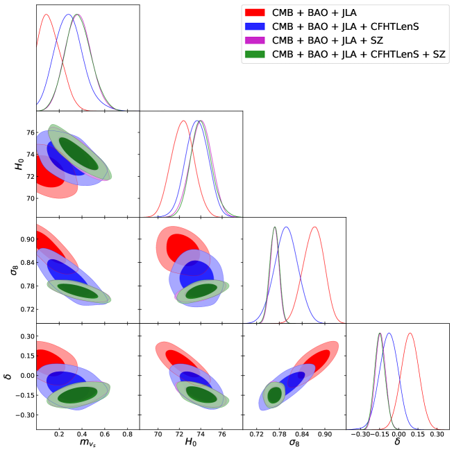
As a generalization of the $\nu$IVCDM model, it is natural to investigate the cosmological consequences with sterile neutrinos, i.e., we study the $\nu_{s}$IVCDM model, the (3+1) model as described in section III. Since $N_{\rm eff}<3.45$ and $\delta\neq 0$ at $99\%$ CL from CMB + BAO + JLA + CFHTLenS + SZ data in the $\nu$IVCDM model, it would be interesting to investigate the correlation $N_{\rm eff}$, and the mass $m_{\nu_{s}}$ of sterile neutrino with $\delta$, and the other baseline parameters of the $\nu_{s}$IVCDM model. The third column of Table 1 carry the constraints (mean values with 68% errors) on some free parameters of the $\nu_{s}$IVCDM model from four different combinations of data sets as described in the caption of the table. Constraints for $\nu_{s}\Lambda$CDM model are also shown.

Figure 2 shows the one-dimensional marginalized distribution, and 68% and 95% CL regions for some selected parameters of the $\nu_{s}$IVCDM model from the four combinations of data sets as shown in the legend of the figure. We see that the data sets CMB + JLA + BAO again do not provide any significant evidence of interaction in the dark sector. On the other hand, the inclusion of CFHTLenS data does not provide significant deviations on the coupling parameter as $\delta\sim 0$ at 68% CL. But the inclusion of SZ data alone and SZ + CFHTLenS data yield $\delta<0$ at 99% CL. More precisely, we note the coupling parameter in the range $-0.04\leq\delta\leq-0.25$ at $99\%$ CL. This shows again a strong evidence of interaction in the dark sector when the GC data in taken into account. Further, we observe a correlation between $\delta$ and $m_{\nu_{s}}$ in case of the CMB + JLA + BAO data set with and without GC data. The inclusion of GC data brings a correlation between the two parameters. The parameter $\delta$ exhibits correlation with both $H_{0}$ and $\sigma_{8}$. Thus, the larger values of $H_{0}$ and smaller values of $\sigma_{8}$ would push the parameter $\delta$ (with negative values) away from 0. Likewise, correlations among the parameters $m_{\nu_{s}}$, $H_{0}$, and $\sigma_{8}$ can be seen clearly from the Figure 2. From the joint analysis using all the data sets under consideration, we find $m_{\nu_{s}}=0.37^{+0.11}_{-0.11}$ eV at 68% CL.

It is well known that the parameters describing neutrinos can exhibit degeneracy with the other cosmological parameters. In Li , the authors show that there is a strong degeneracy between the spectral index ($n_{s}$) and $N_{\rm eff}$. As discussed in Planck_inflation_2015 ; Planck_inflation_2013 , the $\Lambda$CDM scenario with $n_{s}=1$ and $\Delta N_{\rm eff}\approx 1$ can fit the Planck CMB data. In Verde , the authors considered $N_{\rm eff}$ + $\Lambda$CDM (with $n_{s}=1$), and showed that the model can perfectly fit CMB data. Therefore, we can expect a correlation between the parameters $N_{\rm eff}$, $n_{s}$ and $H_{0}$. The unusual high constraints on $n_{s}$ observed in $\nu_{s}$IVCDM model are surely due to the correlation between $N_{\rm eff}$ and $n_{s}$, which is related to the diffusion damping caused by $N_{\rm eff}$ at high multipoles, that requires $n_{s}\sim 1$ to compensate the suppression. On the other hand, the additional free parameters representing physics beyond the $\Lambda$CDM model can also correlate with these parameters. Thus, the constraints on $n_{s}$ also could be the outcome of that correlation. A detailed analysis of an extended parametric space for cosmological models besides $\Lambda$CDM scenario, including effects on inflation parameters, will be presented in a forthcoming paper eu .

IV.3 Analysis of the tensions on $H_{0}$ and $\sigma_{8}$

Assuming standard $\Lambda$CDM baseline, the Planck collaboration Planck2015 measured $H_{0}=67.27\pm 0.66$ km s^-1 Mpc^-1 that is about two standard deviations away from the locally measured value $H_{0}=73.24\pm 1.74$ km s^-1 Mpc^-1 reported in Riess . Results from Planck collaboration have also revealed around 2$\sigma$ level tension between CMB temperature and the Sunyaev-Zel’dovich cluster abundances measurements on $\sigma_{8}$ parameter given by $\sigma_{8}=0.831\pm 0.013$ Planck2015 and $\sigma_{8}=0.75\pm 0.03$ S8_planck , respectively. Thus, the galaxy cluster measurements prefer lower values of $\sigma_{8}$. In Pourtsidou , it has been argued that interacting dark sector models can reconcile the present tension on $\sigma_{8}$. In the present study, we have observed strong correlation of the coupling parameter $\delta$ with $H_{0}$ and $\sigma_{8}$, in both $\nu$IVCDM and $\nu_{s}$IVCDM models, such that the larger departure of negative $\delta$ values from 0 leads to larger values of $H_{0}$ and smaller values of $\sigma_{8}$. Also, we can see the degeneracy between $\delta$, $H_{0}$, and $\sigma_{8}$ with clarity in Figure 3, where the parametric space $\sigma_{8}-\delta$ coloured by $H_{0}$ values is shown for the $\nu$IVCDM (left panel) and $\nu_{s}$IVCDM (right panel) models. Having a note of these observations, we now proceed to examine whether these models can alleviate the current tensions on $H_{0}$ and $\sigma_{8}$.

Figure 3: Constraints on $\sigma_{8}-\delta$ parametric space coloured by $H_{0}$ values for the $\nu$IVCDM (left panel) and $\nu_{s}$IVCDM (right panel) models from CMB + BAO + JLA + CFHTLenS + SZ data.

Figure 4: 1D marginalized probability distributions of $H_{0}$ and $\sigma_{8}$ for $\nu$IVCDM (upper panel) and $\nu_{s}$IVCDM (lower panel) models. The vertical gray band in left panels corresponds to $H_{0}=73.24\pm 1.74$ km s^-1Mpc Riess while in right panels it corresponds to $\sigma_{8}=0.75\pm 0.03$ S8_planck . CBJ stands for CMB + BAO + JLA.

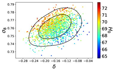
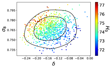
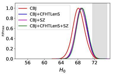
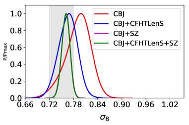
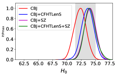
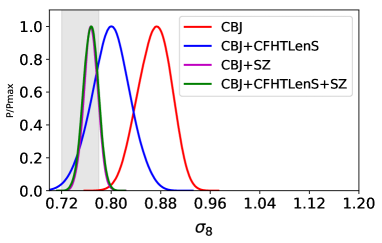
Figure 4 shows 1D marginalized probability distributions of $H_{0}$ and $\sigma_{8}$ for $\nu$IVCDM (upper panel) and $\nu_{s}$IVCDM (lower panel) models. We notice that the tension on $H_{0}$ can not be reconciled marginally in the $\nu$IVCDM model. The plot in upper right panel shows that tension on $\sigma_{8}$ is reconciled perfectly in the $\nu$IVCDM model when the GC data is taken into account for the constraints. See the constraints on $H_{0}$ and $\sigma_{8}$ in second column of Table 1. It is important to mention that we are not taking any prior on $H_{0}$ in our analysis. From the plot in lower left panel, we notice that the tension on $H_{0}$ is reconciled in $\nu_{s}$IVCDM model when constrained with any of the four data combinations under consideration. This is due to the positive correlation between $N_{\rm eff}$ and $H_{0}$. On the other hand, the tension on $\sigma_{8}$ is reconciled in $\nu_{s}$IVCDM model when it is constrained by including GC data from SZ alone or SZ + CFHTLenS (see the plot in the lower right panel of Figure 4). Thus, the $\nu_{s}$IVCDM model can alleviate the tensions on both the parameters $H_{0}$ and $\sigma_{8}$, with the coupling parameter $\delta\neq 0$ at 99% CL from the full data set under consideration. A detailed and clear exposition of all the values of these parameters in $\nu_{s}$IVCDM model, from all the four data combinations, can be seen in the third column of table 1.

Table 2: Summary of the $\Delta\rm AIC$ values and its interpretation. Here, $\Delta\rm AIC_{\nu}=AIC(\nu\Lambda CDM)-AIC(\nu IVCDM)$ and $\Delta\rm AIC_{\nu_{s}}=AIC(\nu_{s}\Lambda CDM)-AIC(\nu_{s}IVCDM)$.

Data combination	$\Delta\rm AIC_{\nu}$	$\Delta\rm AIC_{\nu_{s}}$
CMB+BAO+JLA	$-1.10$ (no evidence)	$-1.58$ (no evidence)
CMB+BAO+JLA+CFHTLenS	3.84 (positive evidence)	0.62 (no evidence)
CMB+BAO+JLA+SZ	14.84 (very strong evidence)	9.82 (strong evidence)
CMB+BAO+JLA+CFHTLenS+SZ	16.18 (very strong evidence)	9.21 (strong evidence)

It is usual in the literature to reconcile both the tensions by assuming an extended parametric space of $\Lambda$CDM model. The authors in T4 argue that the tension must be resolved by considering systematics effects on important data, or by new physics beyond the introduction of massive (active or sterile) neutrinos. Here we have demonstrated the reconciliation of both the tensions, while observing the signs of a new physics, viz., the coupling parameter of the dark sector is non-zero up to $99\%$ CL.

Finally, we close the observational analysis section by comparing the statistical fit obtained using the standard information criteria via Akaike Information Criterion (AIC) Akaike ; Burnham

$$\rm AIC=-2\ln L+2d=\chi^{2}_{min}+2d,$$ (3)

where $L=\exp(-\chi^{2}_{min}/2)$ is the maximum likelihood function and $d$ is the number of model parameters.

We need a reference model with respect to which the comparisons will be performed. In this regard, the obvious choice is the $\Lambda$CDM cosmology with and without sterile neutrinos in comparison with IVCDM model with and without sterile neutrinos.

The thumb rule of AIC reads as follows: If $\Delta\rm AIC\leq 2$, then the models are compatible, i.e., statistically indistinguishable from each other. The range $2\leq\Delta\rm AIC\leq 6$ tells a positive evidence, $6\leq\Delta\rm AIC\leq 10$ implies a strong evidence and $\Delta\rm AIC\geq 10$ infers a very strong evidence.

Table 2 summarizes the comparison between the models for each analysis. Without loss of generalization, these results are also valid with other standard criteria in the literature evaluating directly the values of $\chi^{2}_{min}$. From Table 2, we notice that the inclusion of SZ data to the other data sets in the fit leads to strong evidence. It is in line with the results in Table 1 where one may observe that the $\chi^{2}_{min}$ values increase significantly with the inclusion of SZ data. From Table 1 one may further notice that the two models with sterile neutrino fit with larger $\chi^{2}_{min}$ values in comparison to the other two models whereas the interacting vacuum energy models fit with smaller $\chi^{2}_{min}$ values in comparison to the non-interacting ones. It is well known that a model with $\Delta N_{\rm eff}=1$ can be disfavored up to 3$\sigma$ CL when confronted with the observational data. For instance, Planck team CMB using CMB + BAO data excluded the possibility $N_{\rm eff}=4$ at 99% CL, in comparison to the case where $N_{\rm eff}$ is taken as a free parameter. Thus, it is reasonable to expect that the value of $\chi^{2}_{min}$ increases in our analyzes too where we fix $\Delta N_{\rm eff}=1$. In Table 1, we notice that the joint analysis yields, $\Delta\chi^{2}=10.68$ (for $\Lambda$CDM model) and $\Delta\chi^{2}=14.16$ (for the interacting vacuum energy model), when compared the 3 + 1 neutrino model to the case where $N_{\rm eff}$ is free parameter. On the other hand, analyzing the joint analysis fit only within the 3 + 1 neutrino model scenario, we can notice that the vacuum decay model improves the fit by $\Delta\chi^{2}=5.61$ when compared with the $\Lambda$CDM model.

V Conclusions

We have shown how an extended parametric space with massive neutrinos can influence the observational constraints on a coupling between DM and DE, where DE is characterized by a cosmological constant, i.e., an interacting vacuum energy scenario. Considering two neutrino scenarios via $\nu$IVCDM and $\nu_{s}$IVCDM models, we have found that the inclusion of GC data to CMB + BAO + JLA data considerably improves the observational constraints in favor of an interaction in the dark sector. In particular, both the models yield the coupling parameter $\delta<0$ at 99% CL when constrained by including the GC data. Thus, we conclude that the GC data enforces almost a certain interaction in the dark sector where the DM decays into vacuum energy, within the framework of each of the two models under consideration. We have demonstrated how the coupling parameter $\delta$ correlates with other parameters, and how the current tensions on the parameters $H_{0}$ and $\sigma_{8}$ can be reconciled in the two models.

Recent anomalies in neutrino experiments can be explained by neutrino oscillations if the standard three-neutrino mixing is extended with the addition of light sterile neutrinos, which can give us important information on the new physics beyond the standard model. In the present study, we have studied the so-called (3 + 1) neutrinos model, i.e., the $\nu_{s}$IVCDM model, and also we have found an evidence for a coupling between DM and DE at 99% CL. If future neutrino experiments confirm the existence of light sterile neutrinos, this may lead to a possible evidence for a non-minimal coupling between the dark components on cosmological scales.

In the present work, we have considered GC data from $\sigma_{8}-\Omega_{m}$ plane ($S_{8}$ data is usually used in the literature) and we noticed a strong correlation with the coupling parameter between DM and DE. It is important to mention that this data set consists of a useful parameterization, but a detailed analysis using the full likelihood (direct information from the power spectrum) can lead to more accurate and useful results. In general, the GC data depends on non-linear physics. Further, it is also well known that massive neutrinos play an important role on small scale (non-linear scale). Thus, investigation of interacting DE models within this perspective may be worthwhile.

Future and more accurate measurements from important cosmological sources, in particular large scale structure (including non-linear scale) and CMB, and of neutrino properties including mass hierarchy, effective number of species, as well as the sum of the active neutrino masses, can shed light on the possible interaction in the dark sector.

References

- (1) A. G. Reiss et al., Astron. J. 116, 1009 (1998). [arXiv:9805201]
- (2) S. J. Perlmutter et al., Astrophys. J. 517, 565 (1999). [arXiv:9812133]
- (3) R. A. Battye, T. Charnock and A. Moss, Phys. Rev. D 91, 103508 (2015). [arXiv:1409.2769]
- (4) G. E. Addison, Y. Huang, D. J. Watts, C. L. Bennett, M. Halpern, G. Hinshaw, and J. L. Weiland, Astrophys. J. 818, 132 (2016). [arXiv:1511.00055]
- (5) J. L. Bernal, L. Verde and A. G. Riess, JCAP 1610, 019 (2016). [arXiv:1607.05617]
- (6) B. Leistedt, H. V. Peiris, and L. Verde, Phys. Rev. Lett. 113, 041301 (2014). [arXiv:1404.5950]
- (7) J. W. Hu, R. G. Cai, Z. K. Guo, and B. Hu, JCAP 1405, 020 (2014). [arXiv:1401.0717]
- (8) S. Weinberg, Rev. Mod. Phys. 61, 1 (1989).
- (9) T. Padamanbhan, Class. Quant. Grav. 19, L167 (2002). [arXiv:0204020]
- (10) T. Padamanbhan, Phys. Rep. 380, 235 (2003). [arXiv:0212290]
- (11) R. Bousso, Gen. Relativ. Gravit. 40, 607 (2008). [arXiv:0708.4231]
- (12) Yu. L. Bolotin, A. Kostenko, O. A. Lemets, and D.A. Yerokhin, Int. J. Mod. Phys. D 24, 1530007 (2015). [arXiv:1310.0085]
- (13) B. Wang, E. Abdalla, F. Atrio-Barandela, and D. Pavón, Rep. Prog. Phys. 79, 096901 (2016). [arXiv:1603.08299]
- (14) V. Salvatelli, N. Said, M. Bruni, A. Melchiorri, and D. Wands, Phys. Rev. Lett. 113, 181301 (2014). [arXiv:1406.7297]
- (15) J. Sola, A. G. Valent and J. C. Perez, Astrophys. J. Lett. 811, L14 (2015). [arXiv:1506.05793]
- (16) J. Sola, A. G. Valent and J. C. Perez, arXiv:1602.02103.
- (17) C. Pigozzo, S. Carneiro, J. S. Alcaniz, H. A. Borges, and J. C. Fabris, JCAP 1605, 022 (2016). [arXiv:1510.01794]
- (18) M. G. Richarte, and L. Xu, arXiv:1506.02518.
- (19) J. Väliviita, and E. Palmgren, JCAP 1507, 015 (2015). [arXiv:1504.02464]
- (20) E. G. M. Ferreira, J. Quintin, A. A. Costa, E. Abdalla, and B. Wang, JCAP, 05 (2016) 022. [arXiv:1412.2777]
- (21) R. Murgia, S. Gariazzo, and N. Fornengo, JCAP 1604, 014 (2016). [arXiv:1602.01765]
- (22) C. Bruck and J. Mifsud, arXiv:1709.04882.
- (23) W. Yang, N. Banerjee and S. Pan, Phys. Rev. D 95, 123527 (2017). [arXiv:1705.09278]
- (24) W. Yang, S. Pan and D. F. Mota, arXiv:1709.00006.
- (25) L. Santos, W. Zhao, E. G. M. Ferreira and J. Quintin, arXiv:1707.06827.
- (26) S. Kumar and R. C. Nunes, arXiv:1709.02384.
- (27) M. C. G. Garcia and M. Maltoni, Phys. Rept. 460 , 1 (2008). [arXiv:0704.1800]
- (28) M. C. G. Garcia, M. Maltoni, and T. Schwetz, Nucl. Phys. B 908, 199 (2016). [arXiv:1512.06856]
- (29) F. Capozzi, E. Lisi, A. Marrone, D. Montanino, and A. Palazzo, Nucl. Phys. B 908, 218 (2016). [arXiv:1601.07777]
- (30) A. Palazzo, Mod. Phys. Lett. A 28, 1330004 (2013). [arXiv:1302.1102].
- (31) K. N. Abazajian et al., arXiv:1204.5379.
- (32) S. Gariazzo, C. Giunti, M. Laveder, Y. F. Li, and E. M. Zavanin, J. Phys. G: Nucl. Part. Phys. 43, 033001 (2016). [arXiv:1507.08204]
- (33) A. D. Dolgov, Phys. Rept. 370, 333 (2002). [arXiv:0202122]
- (34) J. Lesgourgues, and S. Pastor, Phys. Rept. 429, 307 (2006). [arXiv:0603494]
- (35) J. Lesgourgues and S. Pastor, New Journal of Physics 16, 065002 (2014). [arXiv:1404.1740]
- (36) P. A. R. Ade et al., A & A 594, A13 (2016). [arXiv:1502.01589]
- (37) E. D. Valentino et al., arXiv:1612.00021.
- (38) E. D. Valentino and L. M. Houghton, arXiv:1612.08334.
- (39) J. L. Bernal, L. Verde, and A. G. Riess, JCAP 10, 019 (2016). [arXiv:1607.05617]
- (40) M. Wyman, D. H. Rudd, R. A. Vanderveld, and W. Hu, Phys. Rev. Lett. 112, 051302 (2014). [arXiv:1307.7715]
- (41) Adam G. Riess et al., ApJ 826, 56 (2016). [arXiv:1604.01424]
- (42) T. Tram, R. Vallance, and V. Vennin, JCAP 01, 046 (2017). [arXiv:1606.09199]
- (43) J. F. Zhang, Y. H. Li, and X. Zhang, Phys. Lett. B 739, 102 (2014). [arXiv:1408.4603]
- (44) T. Bringmann, J. Hasenkamp, and J. Kersten, JCAP 1407, 042 (2014). [arXiv:1312.4947]
- (45) P. Ko and Y. Tang, Phys. Lett. B 739, 62 (2014). [arXiv:1404.0236]
- (46) X. Chu, B. Dasgupta, J. Kopp, JCAP 1510, 011 (2015). [arXiv:1505.02795]
- (47) M. Archidiacono, S. Gariazzo, C. Giunti, S. Hannestad, R. Hansen, M. Laveder, and T. Tram, JCAP 08, 067 (2016). [arXiv:1606.07673]
- (48) E. Giusarm, M. Corsi, M. Archidiacono, R. de Putter, A. Melchiorri, O. Mena, and S. Pandolfi, Phys. Rev. D 83, 115023 (2011). [arXiv:1102.4774]
- (49) W. Yang, H. Li, Y. Wu, and J. Lu, JCAP 10, 007 (2016). [arXiv:1608.07039]
- (50) F. E. M. Costa, E. M. Barboza, Jr. and J. S. Alcaniz, Phys. Rev. D 79, 127302 (2009). [arXiv:0905.0672]
- (51) P. C. Ferreira, J. C. Carvalho, and J. S. Alcaniz, Phys. Rev. D 87, 087301 (2013). [arXiv:1212.2492]
- (52) R. C. Nunes, S. Pan, and E. N. Saridakis, Phys. Rev. D 94, 023508 (2016). [arXiv:1503.04113]
- (53) G. S. Sharov, S. Bhattacharya, S. Pan, R. C. Nunes and S. Chakraborty, Mon. Not. R. Astron. Soc. 466, 3497 (2017). [arXiv:1701.00780]
- (54) R. C. Nunes and E. M. Barboza, Gen. Rel. Grav. 46 1820 (2014). [arXiv:1404.1620]
- (55) W. Yang, N. Banerjee and S. Pan, arXiv:1705.09278.
- (56) E. D. Valentino, A. Melchiorri and O. Mena, Phys. Rev. D 96, 043503 (2017). [arXiv:1704.08342]
- (57) C. Caprini and N. Tamanini, JCAP 10, 1610 006 (2016). [arXiv:1607.08755]
- (58) F. F. Bernardi and R. G. Landim, Eur. Phys. J. C 77 290 (2017). [arXiv:1607.03506]
- (59) L. Feng and X. Zhang, JCAP 08 072 (2016). [arXiv:1607.05567]
- (60) C. van de Bruck, J. Mifsud and J. Morrice, Phys. Rev. D 95, 043513 (2017), arXiv:1609.09855.
- (61) S. Kumar and R. C. Nunes, Phys. Rev. D 94, 123511 (2016). [arXiv:1608.02454]
- (62) J. H. He, B. Wang and E. Abdalla, Phys. Lett. B 671, 139 (2009). [arXiv:0807.3471]
- (63) Y. Wang, D. Wands, L. Xu, J. De-Santiago, and A. Hojjati, Phys. Rev. D 87, 083503 (2013). [arXiv:1301.5315]
- (64) D. Wands, J. D. Santiago and Y. Wang, Class. Quant. Grav. 29, 145017 (2012). [arXiv:1203.6776]
- (65) C. P. Ma and E. Bertschinger, Astrophys. J. 455, 7 (1995). [arXiv:9506072]
- (66) Planck collaboration: P. A. R. Ade et al., A & A 594, A13 (2016). [arXiv:1502.01589]
- (67) F. Beutler, C. Blake, M. Colless, D. H. Jones, L. Staveley- Smith, L. Campbell, Q. Parker, W. Saunders, and F. Watson, MNRAS 416, 3017 (2011). [arXiv:1106.3366]
- (68) A. J. Ross, L. Samushia, C. Howlett, W. J. Percival, A. Burden, and M. Manera, MNRAS 449, 835 (2015). [arXiv:1409.3242]
- (69) L. Anderson et al., MNRAS 441, 24 (2014). [arXiv:1312.4877]
- (70) A. Font-Ribera, et al., JCAP 5, 27 (2014). [arXiv:1311.1767]
- (71) M. Betoule et al., (SDSS collaboration), Astron. Astrophys. 568, A22 (2014). [arXiv:1401.4064]
- (72) Planck collaboration: P. A. R. Ade et al., A & A 594, A24 (2016). [arXiv:1502.01597]
- (73) C. Heymans et al., MNRAS 432, 2433 (2013). [arXiv:1303.1808]
- (74) D. Blas, J. Lesgourgues, and T. Tram, JCAP 07, 034 (2011). [arXiv:1104.2933]
- (75) B. Audren, J. Lesgourgues, K. Benabed and S. Prunet, JCAP 02, 001 (2013). [arXiv:1210.7183]
- (76) A. Gelman and D. Rubin, Inference from iterative simulation using multiple sequences, Statistical Science 7, 457 (1992).
- (77) https://github.com/cmbant/getdist
- (78) H. Li, J. Q. Xia, and X. Zhang, Phys. Dark Univ. 2, 188 (2013). [arXiv:1303.3428]
- (79) Planck collaboration: P. A. R. Ade et al., A & A 594, A20 (2016). [arXiv:1502.02114]
- (80) Planck collaboration: P. A. R. Ade et al., Astron. Astrophys. 571, A22 (2014). [arXiv:1303.5082]
- (81) L. Verde, S. M. Feeney, D. J. Mortlock, and H. V Peiris, JCAP 09, 013 (2013). [arXiv:1307.2904]
- (82) S. Kumar and R. C. Nunes, [In prep.].
- (83) Planck collaboration: P. A. R. Ade et al. A & A 571, A20 (2014). [arXiv:1303.5080]
- (84) A. Pourtsidou and T. Tram, Phys. Rev. D 94, 043518 (2016). [arXiv:1604.04222]
- (85) H. Akaike, A new look at the statistical model identification, IEEE Transactions on Automatic Control, 19, 716 (1974).
- (86) K.P. Burnham and D.R. Anderson, Model selection and multimodel inference (Springer, New York, 2002).