Diffractive scattering on the deuteron

Abstract

High-mass diffractive production of protons on the deuteron target is studied in the perturbative QCD in the BFKL approach. Leading order rearrangement contribution and the standard triple pomeron (the impulse approximation) are studied. In the perturbative limit $\alpha_{s}\to 0$ the rearrangement contribution dominates. Numerical estimates at realistic values of $\alpha_{s}$ and energies strongly depend on assumptions made about the behavior of the pomeron attached to the proton due to unitarization. They indicate that irrespective of these assumptions in the realistic situation the rearrangement and triple pomeron contributions turn out to be of comparable magnitude due to large dimensions of the deuteron.

1 Introduction

In the perturbative QCD collisions on heavy nuclear targets have long been the object of extensive study. In the BFKL approach the structure function of DIS on a heavy nuclear target is given by a sum of fan diagrams in which BFKL pomerons propagate and split by the triple pomeron vertex  [1, 2]. This sum satisfies the well-known Balitski-Kovchegov equation derived earlier in different approaches  [3, 4]. The corresponding inclusive cross-sections for gluon production were derived in  [5, 6]. Description of nucleus-nucleus collisions has met with less success. For collision of two heavy nuclei in the framework of the Color Glass Condensate approach numerical Monte Carlo methods were applied  [7, 8, 9]. Analytical approaches however have only given modest approximate results  [10, 11, 12]. To understand the problem one of the authors (M.A.B) turned to the simplest case of nucleus-nucleus interaction, namely the deuteron-deuteron collisions  [13, 14]. It was found that in this case the diagrams which give the leading contribution are different from the heavy nucleus case and include non-planar diagrams subdominant in $1/N_{c}$ where $N_{c}$ is the number of colors.

In this paper we continue our study of interactions with the deuteron target extending it to the high-mass diffractive production. Diffraction production of a heavy nucleus off the virtual photon was studied long ago  [15] where the evolution equation was constructed for the cross-section integrated over all variables of the produced nucleus. In our case we concentrate on the projectile rather than on the diffractively produced object. We change the virtual photon to the deuteron and the heavy nucleus to the proton with a given momentum. The diffractive production of protons by the deuteron projectile with a large missing mass $M$ is illustrated in Fig. 1. It is assumed that both $M$ and $s$ are large but $M^{2}/s<<1$ so that the deuteron-pomeron amplitude can be given by the pomeron exchanges. In the BFKL, basically perturbative, approach it is assumed that the QCD coupling constant $g$ is small but the overall rapidity $Y$ is large, so that the product $N_{c}g^{2}Y$ is of the order unity or larger. In the BFKL approach one sums all powers of $N_{c}g^{2}Y$ considering $N_{c}g^{2}<<1$. To classify contributions to the diffractive cross-section by their order of magnitude one has to decide whether coupling of the BFKL pomeron to the proton carries a small $g^{2}$ or not. Modeling the proton by an ”onium” consisting of a quark-daiquiri pair at close distance between them (and so of large relative momentum) one may think that the coupling is just $g^{2}$ and small. On the other hand the realistic proton does not contain large relative momenta of its constituents on the average. Then one has no reason to ascribe any smallness to its coupling to the pomeron.

Thus depending on whether we consider the protons on the average (case A) or their hard cores (case B) the order of various contributions will be different.

In case A one forgets about the couplings to the targets. Then the leading contribution is given by the color rearrangement diagram Fig. 2.

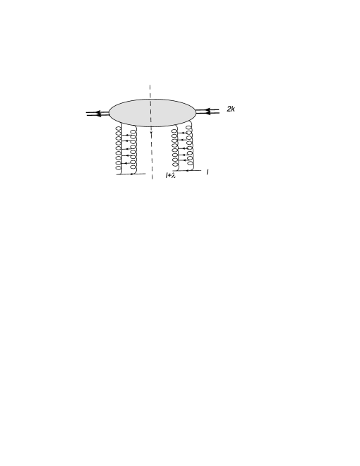
Figure 1: Diffractive production by the deuteron

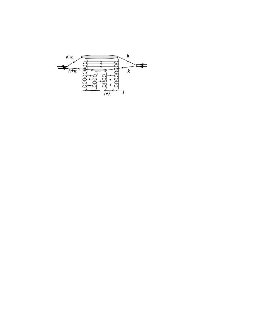
Figure 2: Lowest order color rearrangement contribution

In the lowest order $N_{c}^{2}$ it does not involve any interactions of between the regions. However this gives no contribution to the high-mass diffractive scattering. This contribution comes only in the next order $N_{c}^{3}g^{2}$: Introducing new BFKL interaction between them will realize evolution in rapidity and provide additional factors $(N_{c}g^{2}Y)^{n}$, which, as mentioned, will not change the order of magnitude. Note that this contribution corresponds to double scattering and takes into account the deuteron structure

Among the subleading corrections we find, first of all, the expected diagram with the three-pomeron vertex 3,A. Its order is $N_{c}^{4}g^{4}$. So it is smaller that the rearrangement diagram in Fig. 2 by factor $N_{c}g^{2}$. However the same order of magnitude have the diagrams with the first order correction to the rearrangement diagram 3,B and finally contribution from the RR$\to$RRP vertex 3,C. The first two corrections have a single scattering structure, whereas the last has a double scattering structure as the leading rearrangement term Fig. 3,C.

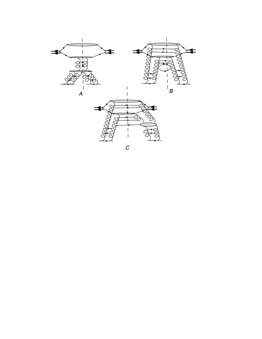
Figure 3: Next-to-leading order contributions: triple pomeron (A), corrections to the reggeon interaction (B), RR$\to$RRP vertex (C).

These estimate are valid in case A when one forgets about the couplings to the proton. In case B, when the proton is represented by its hard core, one has to take into account couplings of the pomerons to the projectile. This gives additional factors $g^{2}$ for single scattering contributions, Figs. 3 A and B and factors $g^{4}$ for double scattering contributions Figs. 2 and 3 C. As a result the tipple pomeron diagram and corrections to the BFKL interaction become comparable to the rearrangement contribution. The ratio of the formers to the latter is now $N_{c}^{2}g^{2}$, which may take any value depending on the relation between $g$ and $1/N_{c}$. Still the contribution from Fig. 3 C remains subdominant.

In this note we shall concentrate on the rearrangement term Fig. 2, which in any case gives a substantial (leading in case A) contribution. The triple pomeron contribution is quite trivial and we calculate it only to compare with the rearrangement term for realistic parameters and energies. As to the rest of the subleading contribution we postpone their discussion for future publications, since their calculation is far from straightforward and needs considerable efforts.

Note that, as is well known, the basic hard contributions we are going to discuss should be supplemented by those coming from additional soft interactions of the participants like shown in Fig. 4 for production amplitudes. In the past they have been widely discussed for various diffraction processes. Their influence can be formulated by introduction of a certain gap survival probability factor $S^{2}$ which should multiply the hard contribution. This factor is obviously non-perturbative. For proton-proton interactions this factor was calculated in  [16, 17, 18, 19] in certain approximation schemes. It turned out to be small, of order 0.1–0.2, and weakly falling with energy. Applied to our deutron case, in all probability, it should be squared. Then to pass to observables we can use the square of the gap survival probability factor $S^{2}$ from  [18, 19].

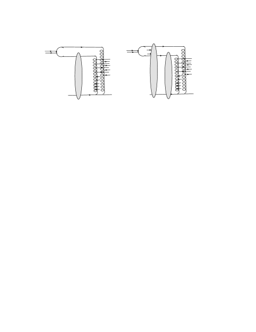
Figure 4: Initial interactions of the participants

Generally the inclusive cross-section of the diffractive proton production $d(2k)+p(l)\to p(l^{\prime})+X$ is given by

$$I(l^{\prime})\equiv\frac{(2\pi)^{3}2l^{\prime}_{-}d\sigma}{dl^{\prime}_{-}d^{2}l^{\prime}_{\perp}}=\frac{1}{s}{\rm Im}{\cal A},$$ (1)

where the forward amplitude ${\cal A}$ corresponds to Fig. 1. Separating the deuteron lines we standardly find (see [1])

$${\cal A}=\frac{1}{m}\int dzF(z)|\psi_{d}(r_{\perp}=0,z)|^{2},$$ (2)

where

$$F(z)=\frac{m}{k_{+}}\int\frac{d\kappa_{+}}{2\pi}H(\kappa_{+})e^{izm\kappa_{+}/k_{+}}.$$ (3)

Here $H$ is the high-energy part of ${\cal A}$, $\kappa_{+}$ is the $+$-component of the transferred momentum $\kappa$ with all other components equal to zero.

For comparison, in the same process with a heavy nucleus projectile, the contribution from the collision with two nucleons is given by (1) with

$${\cal A}=\frac{A(A-1)}{4m}\int d^{2}bdz_{1}dz_{2}F(z_{1}-z_{2})\rho({\bf b},z_{1})\rho({\bf b},z_{2}),$$ (4)

where $\rho({\bf b},z_{1})$ is the nuclear density normalized to unity.

The Glauber approximation corresponds to the contribution which follows when $F(z)$ does not depend on $z$. Then the square of the deuteron wave function converts into the average $<1/2\pi r^{2}>$ and in (4) we find integration over the impact parameter ${\bf b}$ of the square of the profile function $T({\bf b})$. In standard cases the high-energy part contains $\delta(\kappa_{+})$

$$H(\kappa_{+})=2\pi\delta(\kappa_{+})k_{+}D,\ \ {\rm so\ that}\ \ F=mD.$$ (5)

Then for the deuteron

$${\cal A}=D<1/2\pi r^{2}>_{d}$$ (6)

and for a large nucleus

$${\cal A}=\frac{1}{4}A(A-1)D\int d^{2}bT^{2}(\bf b).$$ (7)

The final proton momentum is $l^{\prime}=l+\lambda$. The missing mass is $M^{2}=(2k-\lambda)^{2}=-4k_{+}\lambda_{-}$. So we find

$$\lambda_{-}=-\frac{M^{2}}{4k_{+}}=-\frac{M^{2}}{2s}k_{+},\ \ \lambda_{-}<0.$$ (8)

In the diffractive production, $M^{2}/s<<1$, so that $|\lambda_{-}|<<l_{-}$ (in the c.m. system $k_{+}=l_{-}$). The inclusive cross-section is then expressed via $M^{2}$ and $l^{\prime}_{\perp}$ $l^{\prime}_{\perp}$

$$I(M^{2},l^{\prime}_{\perp})=\frac{(2\pi)^{3}4sd\sigma}{dM^{2}d^{2}l^{\prime}_{\perp}}.$$ (9)

Passing to rapidity $y$ of the outgoing pomerons and $t=l_{\perp}^{2}$ we have

$$J(y,t)=\frac{d\sigma}{dydt}=\frac{M^{2}}{32\pi^{2}s^{2}}{\rm Im}\,{\cal A},$$ (10)

where $M^{2}=M_{0}^{2}\exp(Y-y)$ and $M_{0}\sim 1$ GeV.

2 The impulse approximation

The impulse approximation for our process corresponds to Fig. 3 A and is the sum of cross-sections off the proton and deuteron, each given by the triple pomeron contribution. Although, as mentioned, for the deuteron projectile it may well be subleading, we present it here because it is obviously expected from the start and widely discussed. This cross-section is a sum of contributions from the proton and neutron components of the deuteron

$$J_{impulse}=J_{p}+J_{n}.$$ (11)

Here for each contribution

$$J(y,t)=\frac{N_{c}^{4}g^{4}}{4(2\pi)^{7}}\int\frac{d^{2}r_{12}d^{2}r_{23}}{r_{12}^{2}r_{23}^{2}r_{13}^{2}}P_{y}(\lambda,r_{12})P_{y}(-\lambda,r_{23})e^{i\lambda r_{31}}r_{13}^{4}\nabla_{13}^{4}P_{Y-y}(0,r_{13}).$$ (12)

where $P_{y}(\lambda,r_{12})$ is the pomeron attached to the nucleon with the total transverse momentum $\lambda$ and transverse distance between its reggeon components $r_{12}$.

For simplicity we concentrate on proton emission in the forward direction, $\lambda_{\perp}=0$. Then expression (12) can be simplified by introducing

$$\delta^{2}(r_{12}+r_{23}+r_{31})=\frac{1}{(2\pi)^{2}}\int d^{2}qe^{i(r_{12}+r_{23}+r_{31})}.$$

Integrating over $r_{12}$, $r_{23}$ and $r_{31}$ we get

$$J_{t}(y,t=0)=\frac{N_{c}^{4}g^{4}}{2(2\pi)^{7}}\int d^{2}q\psi^{2}_{y}(q)\chi_{Y-y}(q),$$ (13)

where

$$\psi_{y}(q)=\int\frac{d^{2}r}{r^{2}}e^{iqr}P_{y}(r),\ \ \chi_{Y-y}(q)=\nabla_{q}^{2}q^{4}\nabla_{q}^{2}\psi_{Y-y}(q).$$ (14)

and all pomerons are taken in the forward direction.

3 Leading order contribution

3.1 The rearrangement amplitude

The leading order contribution corresponds to the diagram shown in Fig. 2. It is given by a particular cut of the amplitude for the collision of the deuteron with two targets, calculated in the forward direction in  [13]. After cancelations of infrared divergent terms, without energetic factors and in the purely transverse form the corresponding high-energy part is given by the sum of two terms

$$H_{1}=-i\frac{\partial}{\partial y}\int_{0}^{y}dy^{\prime}\int\frac{d^{2}q}{(2\pi)^{2}}{\tilde{P}}^{2}_{y-y^{\prime}}(q){\tilde{P}}^{2}_{y^{\prime}}(q)$$ (15)

and

$$H_{2}=-2i\int_{o}^{y}dy^{\prime}\int\frac{d^{2}qd^{2}q^{\prime}}{(2\pi)^{4}}{\tilde{h}}(q,q^{\prime}|q^{\prime},q){\tilde{P}}_{y-y^{\prime}}(q){\tilde{P}}_{y-y^{\prime}}(q^{\prime}){\tilde{P}}_{y^{\prime}}(q){\tilde{P}}_{y^{\prime}}(q^{\prime}),$$ (16)

which correspond to direct sewing of pomerons Fig. 5 and one interaction between different pomerons, Fig. 6. Here ${\tilde{P}}_{y}(q)$ is the forward pomeron at rapidity $y$.

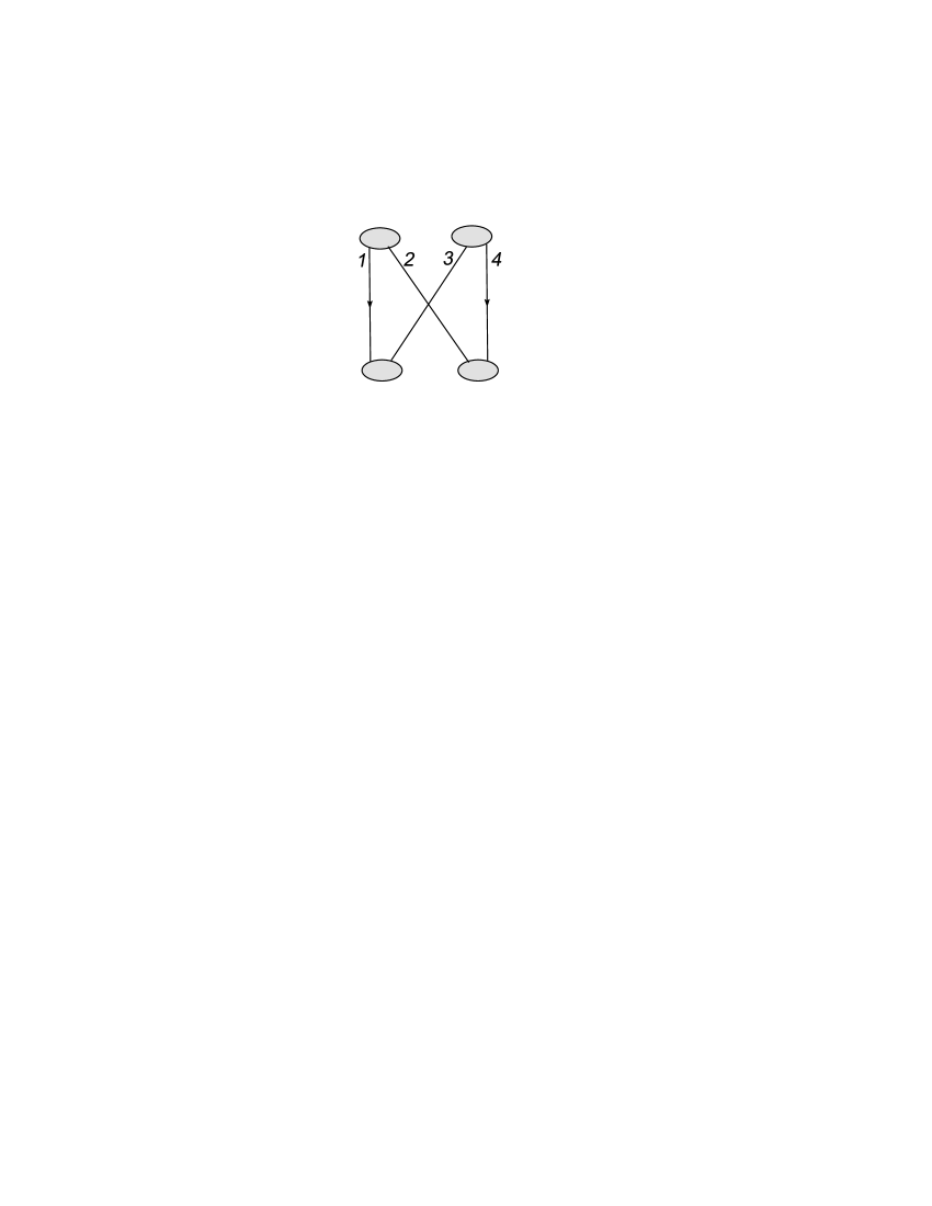
Figure 5: Diagram with the redistribution of color and no interactions between the pomerons of the projectile and target

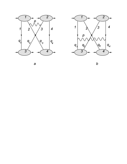
Figure 6: Diagrams with the redistribution of color and one interaction between the pomerons of the projectile and target

In (15) and (16) both the BFKL Hamiltonian ${\tilde{h}}$ and pomerons ${\tilde{P}}$ are taken in the form symmetric respective to the initial and final states. For the non-forward direction they are related to the standard Hamiltonian $h$ and pomerons $P$ as

$${\tilde{P}}(q_{1},q_{2})=q_{1}q_{2}P(q_{1},q_{2}),\ \ {\tilde{h}}(q^{\prime}_{1},q^{\prime}_{2}|q_{1},q_{2})=q^{\prime}_{1}q^{\prime}_{2}h(q^{\prime}_{1},q^{\prime}_{2}|q_{1},q_{2})q_{1}^{-1}q_{2}^{-1}$$ (17)

with

$${\tilde{h}}(q^{\prime}_{1},q^{\prime}_{2}|q_{1},q_{2})=\tilde{v}(q^{\prime}_{1},q^{\prime}_{2}|q_{1},q_{2})-(2\pi)^{4}\delta^{2}(q_{1}-q^{\prime}_{1})\delta^{2}(q_{q}-q_{q}^{\prime})\Big{(}\omega(q_{1})+\omega(q_{2})\Big{)},$$ (18)

where $\omega(q)$ is the gluon Regge trajectory and the BFKL interaction is taken as

$$\tilde{v}(q^{\prime}_{1},q^{\prime}_{2}|q_{1},q_{2})=\frac{g^{2}}{2\pi q_{1}q_{2}q^{\prime}_{1}q^{\prime}_{2}}\Big{(}\frac{q_{1}^{2}{q^{\prime}_{2}}^{2}+q_{2}^{2}{q^{\prime}_{1}}^{2}}{(q_{1}-q^{\prime}_{1})^{2}}-(q_{1}+q_{2})^{2}\Big{)}.$$ (19)

Here the momenta are transverse Euclidian , so that $q^{2}\equiv{\bf q}^{2}$. As compared to  [13] we have added factor $-i$ corresponding to transition from the $S$-matrix to the amplitude.

For our purpose we somewhat transform these expressions. First we consider the corresponding non-forward expressions providing each pomeron with its two momenta. Next we perform the differentiation in (15) to transform

$$H_{1}=H_{1}^{(0)}+H_{1}^{(1)},$$

where

$$H_{1}^{(0)}=-i\int d\tau{\tilde{P}}_{0}(4,1){\tilde{P}}_{0}(3,2){\tilde{P}}_{y}(4,3){\tilde{P}}_{y}(1,2)$$ (20)

and

$$H_{1}^{(1)}=i\int_{0}^{y}dy^{\prime}\int d\tau\Big{(}{\tilde{h}}_{41}+{\tilde{h}}_{32}\Big{)}{\tilde{P}}_{y-y^{\prime}}(4,1){\tilde{P}}_{y-y^{\prime}}(3,2){\tilde{P}}_{y^{\prime}}(4,3){\tilde{P}}_{y^{\prime}}(1,2),$$ (21)

Here $\tau$ is the transverse phase volume (different in (20) and (21)). Notation ${\tilde{P}}_{y}(1,2)$ means the pomeron at rapidity $y$ depending on two transverse momenta of the reggeons $k_{1}$ and $k_{2}$. In (21) it is understood that each Hamiltonian is to be applied to the pomeron depending on the relevant momenta..

Taking part $H_{2}$. in the non-forward direction we find the total transverse high energy part as

$$H^{tot}=H_{1}^{(0)}+H,$$

where

$$H=-i\int_{0}^{y}dy^{\prime}\int d\tau\Big{(}{\tilde{h}}_{13}+{\tilde{h}}_{42}-{\tilde{h}}_{41}-{\tilde{h}}_{32}\Big{)}$$

$$\times{\tilde{P}}_{y-y^{\prime}}(4,1){\tilde{P}}_{y-y^{\prime}}(3,2){\tilde{P}}_{y^{\prime}}(4,3){\tilde{P}}_{y^{\prime}}(1,2).$$ (22)

3.2 Leading order diffractive production

We begin with term $H_{1}^{(0)}$, which graphically is illustrated in Fig. 7. One observes that in the intermediate state we have only contributions with small values of $M^{2}$ contained in $P_{0}(4,1)$ and $P_{0}(3,2)$. So this term does not give any contribution to diffractive production at large $M^{2}$ and we are left with only the integral term in (22).

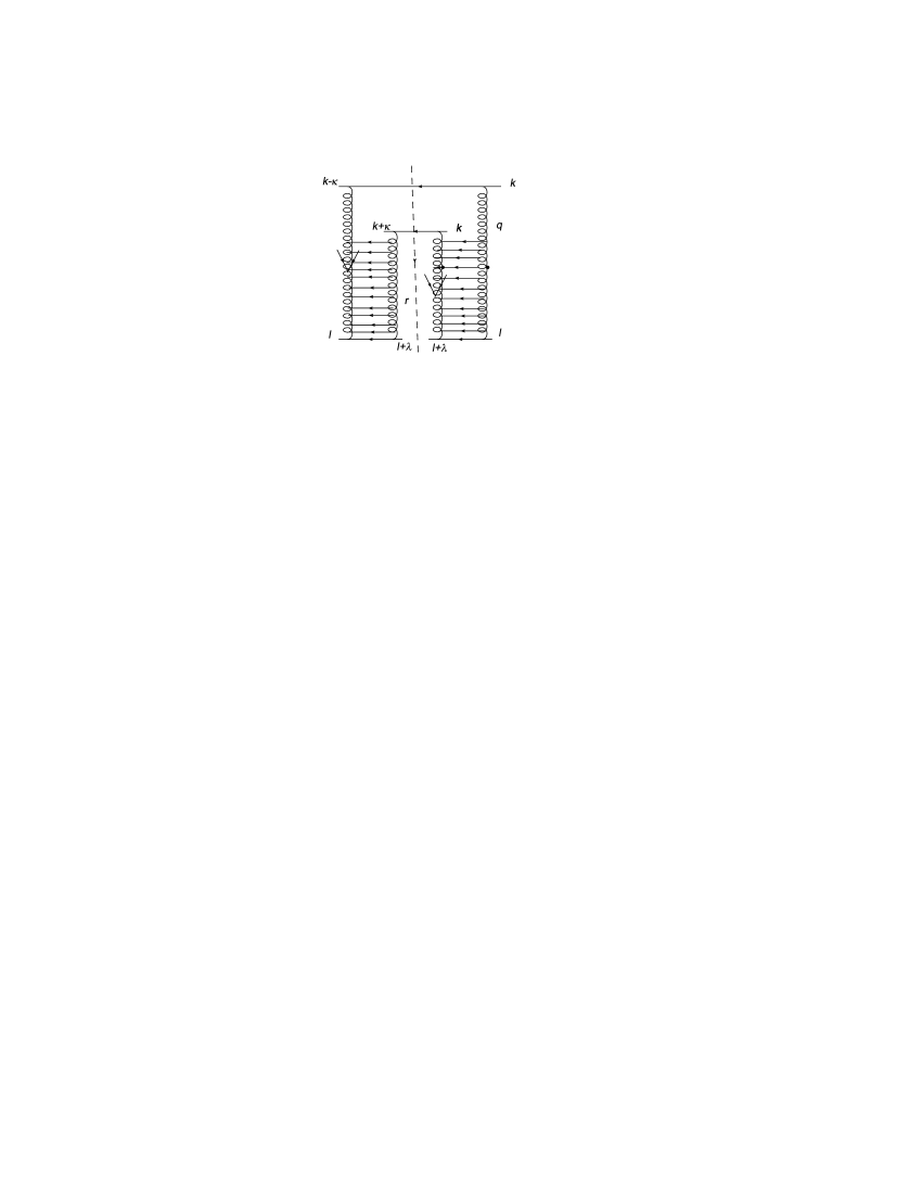
Figure 7: Term $H_{1}^{(0)}$

To find the relevant energetic factors it will be necessary to restore the initial integrations over the 4 momenta taking into account the four impact factors of the pomerons in (22). For simplicity we choose quarks for these impact factors, remove evolution inside the pomerons. We also take into account both direct and crossed contributions to the outgoing pomerons. Then we find for the transverse part (dropping the gluon trajectories in ${\tilde{h}}$, canceled in the sum of four ${\tilde{h}}$)

$$H_{\perp}=-i\int_{0}^{y}dy^{\prime}\int d\tau\Big{(}{\tilde{v}}_{13}+{\tilde{v}}_{24}-{\tilde{v}}_{14}-{\tilde{v}}_{23}\Big{)}$$

$$\times{\tilde{P}}_{y-y^{\prime}}(4,1){\tilde{P}}_{y-y^{\prime}}(3,2){\tilde{P}}_{y}^{\prime}(4,3){\tilde{P}}_{y}^{\prime}(1,2),$$ (23)

where we indicated by the index $\perp$ that this is only the transverse part, which should be multiplied by the appropriate energetic factor. Terms with ${\tilde{h}}_{23}$ and ${\tilde{h}}_{13}$ are illustrated by diagrams A and B in Fig. 8 respectively.

Figure 8: LO contribution with terms ${\tilde{v}}_{23}$ (A) and ${\tilde{v}}_{13}$ (B) in (23) without evolution

Consider the term with ${\tilde{v}}_{23}$ in (23), shown in Fig8,A. We have 6 transferred momenta $q_{2}$, $q_{3}$, $r_{2}$, $r_{3}$, $q_{4}=r_{4}$ and $q_{1}=r_{1}$ related by constraints

$$\kappa=q_{1}+q_{4}=-q_{3}-q_{2},\ \ \lambda=r_{1}+r_{2}=-r_{3}-r_{4}.$$ (24)

So we have two independent transferred momenta, for which we choose $q_{2}$ and $r_{1}$, with others related to them as $q_{3}=-\kappa-q_{2},\ \ r_{2}=\lambda-r_{1},\ \ q_{1}=r_{1},\ \ q_{4}=\kappa-r_{1}.$

Let us study integrations over the 4 independent longitudinal momenta $q_{2\pm}$ and $r_{1\pm}$. The 4 impact factors (with crossed and non-crossed reggeons) give

$$256k_{+}^{4}l_{-}^{4}(2\pi)^{4}\delta(2k_{+}q_{1-})\delta(2k_{+}q_{2}-)\delta(2l_{-}r_{1+})\delta(2l_{-}r_{4+})$$

$$=(2\pi)^{4}4s^{2}\delta(\kappa_{+})\delta(r_{1-})\delta(r_{1+})\delta(q_{2-}).$$ (25)

The four longitudinal integrations go over $q_{2\pm}$ and $r_{1\pm}$. Integration over $q_{+}$ can be changed to that over $p_{+}$. Integrations over $q_{2-}$ and $r_{1\pm}$ are lifted by the $\delta$ functions but the integration over $p_{+}$ remains. In the diagram of Fig. 8,A its transversal part $-iH_{\perp}^{(23)}$, which is just the term with ${\tilde{h}}_{23}$ in (23, is multiplied by the propagator of the intermediate gluon $-i/(p^{2}+i0)$. So the final longitudinal integration is

$$-i\int\frac{dp_{+}}{2\pi(2p_{+}p_{-}+p_{\perp}^{2}+i0)}=-\frac{1}{4p_{-}}.$$

This brings us to the final energetic factor

$$-2\pi\delta(\kappa_{+})4s^{2}\frac{1}{4p_{-}}=2\pi\delta(\kappa_{+})4s^{2}\frac{1}{4\lambda_{-}}=-2\pi\delta(\kappa_{+})4s^{2}\frac{k_{+}}{M^{2}}$$ (26)

and the high-energy part corresponding to Fig. 8,A will be

$$8\pi i\delta(\kappa_{+})N_{c}^{3}g^{2}s^{2}\frac{k_{+}}{M^{2}}H_{\perp}^{(23)}.$$ (27)

Now consider the integration over $y$ in (23). Rapidity $y$ is expressed via the missing mass $M^{2}$, which in turn is expressed via $l^{\prime}_{-}-l_{=}\lambda_{-}$:

$$y=\ln\frac{s}{M^{2}},\ \ M^{2}=-4k_{+}\lambda_{-}.$$ (28)

So we have

$$\int dy=\int\frac{dM^{2}}{M^{2}}=\int\frac{dl^{\prime}_{-}}{l^{\prime}_{-}}$$

and we obtain (10) by removing integration over $y$ and fixing $y$ according to (28).

Next we study the term with ${\tilde{v}}_{13}$ in (23), shown in Fig, 8,B. Here the 6 transferred momenta are $q_{1}$, $q_{2}$, $r_{1}$, $r_{2}$, $q_{3}=r_{3}$ and $q_{4}=r_{4}$, constrained by conditions (24). We take $q_{1}$ and $r_{1}$ as independent momenta. In terms of them

$$q_{4}=r_{4}=\kappa-q_{1},\ \ q_{2}=r_{2}=\lambda-r_{1},\ \ q_{3}=r_{1}-\lambda-\kappa,\ \ r_{3}=q_{1}-\lambda-\kappa.$$ (29)

From impact factors(25) together with (29) we obtain a factor

$$(2\pi)^{4}4s^{2}\delta(q_{1-})\delta(\lambda_{-}-r_{1-})\delta(r_{1+})\delta(\kappa_{+}-q_{1+}).$$ (30)

Note that from (29) it follows

$$p_{+}=q_{1+},\ \ p_{-}=-r_{1-},$$

so that (30) can be rewritten as

$$(2\pi)^{4}4s^{2}\delta(q_{1-})\delta(\lambda_{-}+p_{-})\delta(r_{1+})\delta(\kappa_{+}-p_{+}).$$ (31)

After integration over $q_{1-}$, $r_{1+}$ and $p_{\pm}$ we find the transverse part $-iH_{\perp}^{(13)}$ multiplied by the propagator of the intermediate gluon $-i/(p^{2}+i0)$ in which the longitudinal components of $p$ are fixed:

$$p^{2}+i0=2p_{+}p_{-}+p_{\perp}^{2}+i0=-2\lambda_{-}\kappa_{+}+p_{\perp}^{2}+i0.$$

Factor $-i/(p^{2}+i0)$ can be effectively transformed in a simpler expression if one takes into account that it has to be eventually integrated over $\kappa_{+}$ with the weight $\exp(izm\kappa_{+}/k_{+})$. At $k_{+}\to\infty$ we can neglect this weight to have the integral

$$-i\int\frac{d\kappa+}{p^{2}+i0}=\pi\frac{1}{2\lambda}$$

This is the same result that we would obtain if we substitute

$$-i\int\frac{dp_{+}dp_{-}}{p^{2}+i0}\delta(\kappa_{+}-p_{+})\delta(\lambda_{-}+p_{-})\to 2\pi\delta(\kappa_{+})\frac{1}{4\lambda_{-}}$$ (32)

As a result the corresponding energetic factor becomes identical to (26) and the high-energy part corresponding to Fig. 8,C will be

$$8\pi i\delta(\kappa_{+})N_{c}^{3}g^{2}s^{2}\frac{k_{+}}{M^{2}}H_{\perp}^{(13)}$$ (33)

The remaining interactions ${\tilde{h}}_{14}$ and ${\tilde{h}}_{24}$ in (23) can be studied in a similar manner. In fact the results can be achieved by the interchange of reggeons 1234$\to$3412. So function $D$ in fact reduces to (23) with removed integration over $y$. Thus using the definition (5)

$$D=4iN_{c}^{3}g^{2}s^{2}\frac{1}{M^{2}}\int d\tau_{\perp}\Big{(}{\tilde{v}}_{13}+{\tilde{v}}_{24}-{\tilde{v}}_{23}-{\tilde{v}}_{14}\Big{)}$$

$$\times{\tilde{P}}(y-y^{\prime},q_{1},q_{4}){\tilde{P}}(y-y^{\prime},q_{2},q_{3}){\tilde{P}}(y^{\prime},r_{1},r_{2}){\tilde{P}}(y^{\prime},r_{3},r_{4}),$$ (34)

where

$$y^{\prime}=\ln\frac{s}{M^{2}},\ \ q_{1}+q_{2}=q_{3}+q_{4}=0,\ \ r_{1}+r_{2}=-r_{3}-r_{4}=\lambda$$

and all momenta are understood as purely transverse. With the explicit expressions for ${\tilde{v}}_{ik}$ we get

$$D=8iN_{c}^{3}g^{2}s^{2}\frac{1}{M^{2}}(T_{A}+T_{B}),$$ (35)

where terms $T_{A}$ and $T_{B}$ correspond to Fig. 8 A and B

$$T_{A}=\int\frac{d^{2}q_{1}d^{2}q_{2}}{(2\pi)^{4}}\,\frac{2q_{1}^{6}q_{2}^{2}}{(q_{1}+q_{2})^{2}}P_{Y-y}(q_{1})P_{Y-y}(q_{2})P^{2}_{y}(q_{1})$$ (36)

and

$$T_{B}=-\int\frac{d^{2}q_{1}d^{2}q_{2}}{(2\pi)^{4}}q_{1}^{2}q_{2}^{2}\Big{(}\frac{(q_{1}^{4}+q_{2}^{4})}{(q_{1}+q_{2})^{2}}-(q_{1}+q_{2})^{2}\Big{)}P_{Y-y}(q_{1})P_{Y-y}(q_{2})P_{y}(q_{1})P_{y}(q_{2}).$$ (37)

Rewriting the two terms in $T_{B}$ as $T_{B}^{(1)}+T_{B}^{(2)}$, where

$$T_{B}^{(2)}=\int\frac{d^{2}q_{1}d^{2}q_{2}q_{1}^{2}q_{2}^{2}}{(2\pi)^{4}}(q_{1}+q_{2})^{2}P_{Y-y}(q_{1})P_{Y-y}(q_{2})P_{y}(q_{1})P_{y}(q_{2})$$ (38)

we get in the sum

$$T_{A}+T_{B}=\int\frac{d^{2}q_{1}d^{2}q_{2}q_{1}^{2}q_{2}^{2}}{(2\pi)^{4}(q_{1}+q_{2})^{2}}P_{Y-y}(q_{1})P_{Y-y}(q_{2})\Big{(}P_{y}(q_{1})-P_{Y}(q_{2})\Big{)}\Big{(}q_{1}^{4}P_{y}(q_{1})-q_{2}^{4}P_{y}(q_{2})\Big{)}+T_{B}^{(2)}.$$ (39)

As we observe the infrared singularity at $(q_{1}+q_{2})^{2}=0$ is cancelled btween $T_{A}$ and $T_{B}$. After angular integration we get the final cross-section in the forward direction

$$J_{r}(y,t=0)=\frac{\alpha_{s}N^{3}}{4\pi^{3}}\int_{0}^{\infty}dq_{1}dq_{2}q_{1}^{3}q_{2}^{3}P_{Y-y}(q_{1})P_{Y-y}(q_{2})$$

$$\times\Big{[}\frac{1}{|q_{1}^{2}-q_{2}^{2}|}\Big{(}P_{y}(q_{1})-P_{Y}(q_{2})\Big{)}\Big{(}q_{1}^{4}P_{y}(q_{1})-q_{2}^{4}P_{y}(q_{2})\Big{)}+(q_{1}^{2}+q_{2}^{2})P_{y}(q_{1})P_{y}(q_{2})\Big{]}.$$ (40)

3.3 Evolution

Apart from the next-to-leading corrections to the found cross-section shown in Fig. 3 new contributions will be provided by evolution, that is by extra BFKL interactions among the reggeons. Their immediate effect is to organize the fully-developed pomerons coupled to the projectiles and targets, which actually has been already taken into account in our final formula (34). However evolution will also introduce additional contributions to the propagation of the four intermediate reggeons between the projectiles and targets. In the high-color limit introduction of new BFKL interactions between them will create the so-called BKP state, made of 4 reggeons, coupled to the projectiles and targets by BFKL interactions necessary to transform their two-pomeron structure into an irreducible colorless state, in which the reggeons are located on the cylinder surface. This contribution is schematically shown in Fig. 9.

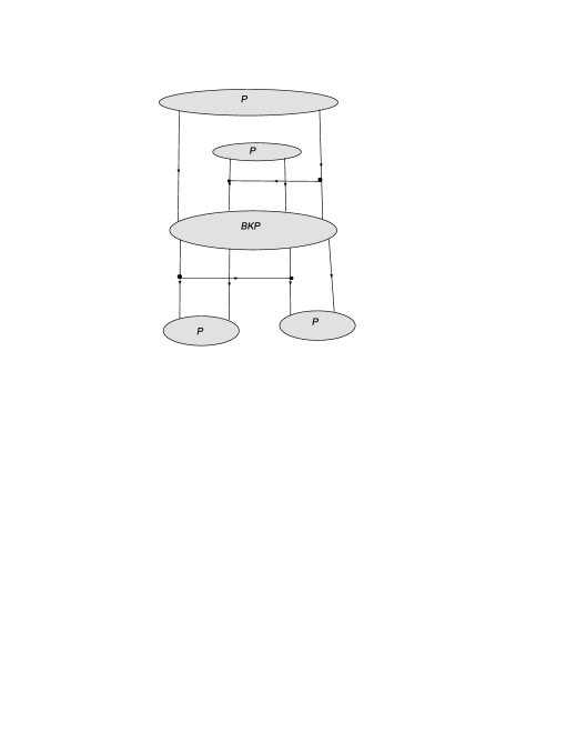
Figure 9: Evolution with formation of the BKP state

It is trivial to write the formal expression for it (see  [13]). However there is not much use from it. On the one hand, the Green functions for the BKP states (except for the odderon) are unknown and in all probability very complicated. On the other hand it is known that the BKP states grow much slowlier with energy than the BFKL pomeron  [23]. Therefore at high energy their rapidity interval will be automatically squeezed to finite rapidities, since the bulk of the contribution will come from the pomerons, which will occupy the whole rapidity interval. Then one can hardly hope to have a small coupling constant inside the BKP state. Within the BFKL approach with a fixed coupling constant adjusted to the overall rapidity interval this constant will be small for the BKP state, so that one has to drop all extra interactions in it. This returns us to the set of next-to-leading corrections in Fig. 3. Thus we do not see any necessity nor possibility to study evolution between the projectiles and targets, at least until we know better the properties of the BKP state.

4 Numerical estimates for the realistic situation

The energy dependence of the cross-section is evidently determined by the behavior of the pomerons attached to the participants. In the strict perturbative approach one takes them to be the standard BFKL pomerons, which grow at large energies as $s^{\Delta}$ where $\Delta=4(N_{c}\alpha_{s}/\pi)\ln 2$. Then at large $s$ the rearrangement contribution $J_{r}$ clearly dominates over the triple pomeron one $J_{t}$ since

$$J_{r}\sim\alpha_{s}\frac{s^{2}}{M_{0}^{4}},\ \ J_{t}\sim\alpha_{s}^{2}\frac{s^{2}}{M^{2}M_{0}^{2}},\ \ \frac{J_{t}}{J_{r}}\sim\alpha_{s}\frac{M_{0}^{2}}{M^{2}},$$ (41)

where one can take $M_{0}=1$ GeV and so $M_{0}^{2}<<M^{2}$. So not only the theoretical smallness of $\alpha_{s}$ but also the energy behavior make the triple pomeron contribution very small relatively.

Passing to concrete calculations we have first to couple the BFKL pomeron to the proton. To this aim we have to introduce the proton dipole density in the momentum space $\rho(k)$ with the property $\rho(0)=0$. We take

$$\rho(k)=\gamma k^{2}e^{-\beta k^{2}}.$$ (42)

The amputated pomeron $\phi_{y}(k)=k^{2}P_{y}(k)$ is then

$$\phi_{y}(k)=\int\frac{d^{2}k^{\prime}}{(2\pi)^{2}}\rho(k^{\prime})g_{y}(k^{\prime},k)=\frac{\gamma}{2\pi\beta k}\int d\nu e^{y\omega(\nu)}k^{2i\nu}\beta^{i\nu}\Gamma(1-i\nu).$$ (43)

Here $g_{y}(k^{\prime}k)$ is the BFKL Green function and $\omega(\nu)$ is the well-known BFKL eigenvalue. At small $\nu$

$$\omega(\nu)=\Delta-a\nu^{2},\ \ \Delta=4\frac{N_{c}\alpha_{s}}{\pi}\ln 2,\ \ a=14\frac{N_{c}\alpha_{s}}{\pi}\zeta(3).$$ (44)

To relate parameters $\gamma$ and $\beta$ to observables we calculate the proton-proton cross-section

$$\sigma(y)=\frac{\gamma^{2}}{8\pi^{2}\beta^{2}}e^{y\Delta}\sqrt{\frac{\pi}{ay}}.$$ (45)

From this we can extract ratio $\gamma/\beta$ by comparison with the experimental data for $\sigma(y)$ at some appropriate $y$. As to $\beta$ it is evidently related to the proton radius $R_{p}$, which we take to be 0.8 fm. We have $\beta=R_{p}^{2}/4$. Both $\gamma$ and $\beta$ are dimensionful

$${\rm dim}\,\alpha=-3,\ \ {\rm dim}\,\beta=-2.$$

In the asymptotic region at large $y$

$$P_{y}(k)=C_{0}\frac{e^{y\Delta}}{\sqrt{y}}\frac{1}{k^{3}}\exp\Big{(}-\frac{\ln^{2}k^{2}}{4ya}\Big{)},\ \ C_{0}=\frac{\gamma}{2\pi\beta}\sqrt{\frac{\pi}{a}}$$ (46)

and for pomerons $\psi$ and $\chi$ introduced by (14) we find in this limit (see Appendix 1.)

$$\psi_{y}(k)=\phi(k)=k^{2}P_{y}(k),\ \ \chi_{y}(k)=9\phi_{y}(k)$$

Note that the scale of $k$ is fixed by the scale of $k^{\prime}$ in the integration with $\rho(k^{\prime})$ and so with the scale of $\beta$. In the following we measure $\beta$ in mbn and so $k^{2}$ in 1/mbn.

Using these asymptotic expressions we find the contribution from the triple pomeron

$$J_{t}^{(1)}(y,t0)=36\pi\alpha_{s}^{2}N_{c}^{4}C_{0}^{3}e^{(Y+y)\Delta}\frac{1}{y\sqrt{Y-y}}I_{t}^{(1)},$$ (47)

where

$$I_{t}^{(1)}=\int_{0}^{\infty}\frac{dq}{q^{2}}\exp\Big{[}-\frac{\ln^{2}q^{2}}{4a}\Big{(}\frac{2}{y}+\frac{1}{Y-y}\Big{)}\Big{]}$$ (48)

and from the rearrangement terms

$$J_{r}^{(1)}(y,t=0)=\frac{\alpha_{s}N_{c}^{3}}{4\pi^{3}}C_{0}^{4}<1/2\pi r^{2}>_{d}e^{2Y\Delta}\frac{1}{y(Y-y)}I_{r}^{(1)}$$ (49)

where

$$I_{r}^{(1)}=\int_{0}^{\infty}\frac{dq_{1}dq_{2}}{q_{1}^{3}q_{2}^{3}}\exp\Big{(}-\frac{\ln^{2}q_{1}^{2}+\ln^{2}q_{2}^{2}}{4a(Y-y)}\Big{)}$$

$$\times\Big{\{}\frac{1}{|q_{1}^{2}-q_{2}^{2}|}\Big{[}q_{2}^{3}\exp\Big{(}-\frac{\ln^{2}q_{1}^{2}}{4ay)}\Big{)}-q_{1}^{3}\exp\Big{(}-\frac{\ln^{2}q_{2}^{2}}{4ay)}\Big{)}\Big{]}$$

$$\times\Big{[}q_{1}\exp\Big{(}-\frac{\ln^{2}q_{1}^{2}}{4ay)}\Big{)}-q_{2}\exp\Big{(}-\frac{\ln^{2}q_{2}^{2}}{4ay)}\Big{)}\Big{]}+(q_{1}^{2}+q_{2}^{2})\exp\Big{(}-\frac{\ln^{2}q_{1}^{2}+\ln^{2}q_{2}^{2}}{4ay)}\Big{)}\Big{\}}.$$ (50)

Integrals $I_{t}^{(1)}$ and $I_{r}^{(1)}$ are convergent both in the ultraviolet and infrared. However in both $I_{t}^{(1)}$ and especially $I_{r}^{(1)}$ the bulk of the contribution comes from extremely low values of $q$, where convergence is achieved due to the damping exponentials $\exp(-c\ln^{2}q^{2})$. As a result the cross-sections turn out to be absurdly large, of order 10¹⁰ bn/Gev². The BFKL approach is certainly not valid in this region. So to be closer to reality we cut the integrations at values $q<\Lambda_{QCD}\sim 0.3$ GeV. We also somewhat diminish the BFKL intercept $\Delta$ to make it more compatible with the data. We choose $\Delta=0.12$ in the hope that unitarity corrections will reduce it to this admissible value. For hard interactions we take $\alpha_{s}=0.2$ and naturally $N_{c}=3$. For the deuteron, using the Hulthen wave function, we find

$$<1/2\pi r^{2}>_{d}=0.0764\ \ 1/{\rm fm}^{2}$$ (51)

The calculated in this manner cross-sections at $Y=19.1$ corresponding to energy 14 TeV are illustrated in Fig. 10 as a function of $Y-y$. We recall that the missing mass squared $M^{2}=\exp(Y-y)$ Gev². As we see the rearrangement cross-section is somewhat smaller than the triple pomeron contribution due to very low value of $<1/2\pi r^{2}>_{d}$. But then the relation between them is very sensitive to the infrared cut: the rearrangement part grows much faster with its lowering.

Figure 10: Diffractive cross-section in the perturbative approach in bn/GeV². The overall rapidity is $Y=19.1$

Still the behavior of the pomerons with all unitarity corrections included should be seriously different from the pure BFKL pomeron, both in the region of high energies and especially of low momenta, where we expect the phenomenon of gluon saturation to take place. So, as an alternative, we shall use expressions for the pomerons based on the latter phenomenon. Prompted by the approximate form for the developed unintegrated gluon densities resulting from the Balitski-Kovchegov evolution equation we take in the coordinate space for the pomeron attached to the proton

$$P_{y}(r)=\frac{2\pi}{g^{2}}S_{\perp}\Big{(}1-e^{-Q_{s}^{2}(y)}\Big{)}.$$ (52)

Here $Q_{s}(y)$ is the proton saturation momentum. Its $y$-dependence was presented in  [12] and is shown in Fig. 11. Factor $S_{\perp}$ is the transverse area of the proton. It appears because the standard unintegrated gluon density is calculated per unit of the transverse area of the target. Factor $2\pi/g^{2}$ is due to different normalization of the unintegrated gluon density and the BFKL pomeron  [22]

Figure 11: $Q_{s}^{2}(y)$ for the proton

With the form (52) both $\psi$ and $\chi$ can be found analytically. If we define

$$x=\frac{q}{2Q_{s}(Y-y)},\ \ \rho=\frac{Q_{s}^{2}(Y-y)}{Q_{s}^{2}(y)}$$ (53)

then we find (see Appendix 2. for details)

$$\psi(q)=-\frac{2\pi^{2}}{g^{2}}S_{\perp}{\rm Ei}(-\rho x^{2}),\ \ \chi(q)=64x^{2}(x^{2}-1)e^{-x^{2}}.$$ (54)

As a result we get the cross-section from the triple pomeron

$$J^{(2)}_{t}(y,t=0)=\frac{N_{c}^{4}}{16\pi\alpha_{s}}S_{\perp}^{3}Q_{s}^{2}(Y-y)I_{t}^{(2)}(\rho),$$ (55)

where

$$I_{t}^{(2)}(\rho)=64\int_{0}^{\infty}dzz(1-z)e^{-z}{\rm Ei}^{2}(-\rho z).$$ (56)

Note that due to operator $\nabla_{q}^{2}q^{4}\nabla_{q}^{2}$ function $\chi(Y-y)$ is not positive for all values of $0<y<Y$ but rather only at certain distance of its ends. Closer to $0$ or $Y$ it becomes negative and pathological (either close to zero or to $-\infty$). This property is apparently the consequence of our choice for the pomeron wave function, which is not conformal invariant, unlike the perturbative BFKL pomeron, for which the above operator is harmless. In the following we exclude from consideration the intervals in $Y-y$ for which $\chi$ is negative.

To calculate the rearrangement contribution (34) we use according to (52)

$$P_{y}(q)=\frac{2\pi}{g^{2}}S_{\perp}\Big{(}(2\pi)^{2}\delta(q)-\frac{\pi}{Q_{s}^{2}(y)}e^{-q^{2}/4Q^{2}_{s}(y)}\Big{)}.$$ (57)

Due to factors $q_{1}^{2}$ and $q_{2}^{2}$ in (40) the $\delta$-terms in (57) give no contribution. So one obtains

$$D=\frac{s^{2}}{M^{2}}\frac{16(2\pi)^{3}N_{c}^{3}}{\alpha_{s}^{3}}S_{\perp}^{4}Q_{S}^{2}(Y-y)I_{r}^{(2)}(\rho),$$ (58)

where

$$I_{r}^{(2)}(\rho)=\rho^{2}\int_{0}^{\infty}x_{1}dx_{1}e^{-(1+\rho)x_{1}}\int_{0}^{x_{1}}x_{2}dx_{2}e^{-(1+\rho)x_{2}}$$

$$\times\Big{\{}\frac{2x_{2}^{2}}{x_{1}-x_{2}}\cosh\Big{(}\rho(x_{1}-x_{2})-1\Big{)}+(x_{1}+x_{2})e^{-\rho(x_{1}-x_{2})}\Big{\}}.$$ (59)

The cross-section is then

$$J_{r}^{(2)}(y,t=0)=\frac{4\pi N_{c}^{3}}{\alpha_{s}^{3}}S_{\perp}^{4}Q_{s}^{2}(Y-y)I_{r}^{(2)}(\rho)<1/2\pi r^{2}>_{d}.$$ (60)

Before any calculations one has the ratio

$$\frac{J_{r}}{J_{t}}=\frac{9N_{c}\alpha_{s}^{2}}{64\pi^{2}S_{\perp}<1/2\pi r^{2}>_{d}}\,\frac{I_{1}(\rho)}{I_{2}(\rho)}.$$ (61)

One observes that for very small $\alpha_{s}$ the rearrangement contribution clearly dominates. However with realistic values of $\alpha_{s}$ and $N_{c}$ the situation changes. Due to the large deuteron dimension, on the one hand, and the relation $I_{1}>>I_{2}$ for realistic rapidities, on the other, the ratio becomes around 10%.

The cross-sections from the triple pomeron and rearrangement calculated in this approach are shown in Fig. 12 for different values of $Y-y$ in bn/GeV².

Figure 12: Diffractive cross sections with gluon saturation in bn/GeV². The overall rapidity is $Y=19.1$

5 Discussion

We have studied the high-mass diffractive proton production off the deuteron. Our attention has been concentrated on the contribution from the color rearrangement diagram, which should dominate the cross-section in the strict perturbative approach. We have derived the corresponding cross-section and demonstarted its infrared finiteness. To compare we also have included the obvious impulse approximation contribution, that is the sum of cross-sections off the proton and neutron with the triple pomeron interaction.

As expected the results crucially depend on the unknown properties of the pomeron coupled to the proton, modified by all sorts of unitarity corrections. With minimal modifications including lowering of the intercept $\Delta$ and cutting in the infrared at momenta of the order $\Lambda_{QCD}$ the results are presented in Fig. 10. More drastic modifications taking into account gluon saturation at low momenta give cross-sections shown in Fig. 12. The results from these two choices are very different in their magnitude, $M^{2}$ -dependence and the relation between the triple pomeron and rearrangement contributions. One hopes that experimental studies may decide for the better choice and thus tell us something on the behavior of the pomeron coupled to the proton. We recall that observable cross-section are to be obtained from ours after multiplication by the squre of survival gap probability factor $S^{2}$ borrowed from  [18, 19]. This will diminish our cross-sections by two orders of magnitude. The main message we can extract from our calculation is that in fact both triple pomeron and rearrangement term give comparable contribution at the LHC energies with a realistic value of the coupling constant for hard processes.

Next step is to take into account, first, evolution between pomerons attached to projectiles and targets (Fig. 9) and, second, higher order corrections indicated in Fig. 3 B and C. Again in the purely perturbative approach they should be small. But for realistic parameters and energies this may be not so. However calculation of these corrections is apparently a highly complicated task and so will be postponed for future investigation.

6 Acknowledgements

This work has been supported by the S.Pertersburg University grant 11.38.223.2015 and RFBR grant 15-02-02097

7 Appendix 1. BFKL pomerons

Elementary eigenfunctions of the BFKL Hamiltonian in the forward direction are the semi-amputated pomerons

$$\phi_{\nu}(k)=\sqrt{2}k^{-1+2i\nu}$$ (62)

normalized according to

$$\int\frac{d^{2}k}{(2\pi)^{2}}\phi_{\nu^{\prime}}^{*}(k)\phi_{\nu}(k)==\delta(\nu-\nu^{\prime})$$ (63)

So the Green function is

$$g_{y}(k^{\prime},k)=\frac{2}{kk^{\prime}}\int d\nu e^{y\omega(\nu)}\Big{(}\frac{k}{k^{\prime}}\Big{)}^{2i\nu}$$ (64)

where at small $\nu$

$$\omega(\nu)=\Delta-a\nu^{2},\ \ \Delta=4\frac{N_{c}\alpha_{s}}{\pi}\ln 2,\ \ a=14\frac{N_{c}\alpha_{s}}{\pi}\zeta(3)$$ (65)

For the triple pomeron contribution we have to know two other pomerons determined via the pomeron $P(r)$ in the coordinate space. First

$$\psi_{y}(q)=\int\frac{d^{2}r}{r^{2}}P_{y}(r)e^{1kr}$$ (66)

To find it we note that

$$k^{2}\nabla_{k}\psi_{y}(k)=k^{2}P_{y}(k)=\phi_{y}(k)$$ (67)

In the $\nu$ representation the $k$ dependence of $\psi_{y}(k)$ is the same as of $\phi_{y}(k)$. So we seek

$$\psi_{\nu}(k)=d_{\nu}k^{-1+2i\nu},\ \ k^{2}\nabla_{k}^{2}\psi_{\nu}(k)=(1-2i\nu)^{2}d_{\nu}k^{-1+2i\nu}$$ (68)

From (67) then

$$\psi_{\nu}(k)=\frac{\phi_{\nu}(k)}{(1-2i\nu)^{2}}$$

so that

$$\psi_{y}(k)=\frac{\alpha}{2\pi\beta k}\int d\nu e^{y\omega(\nu)}k^{2i\nu}\frac{\beta^{i\nu}\Gamma(1-i\nu)}{(1-2i\nu)^{2}}$$ (69)

Finally we need

$$\chi_{y}(r)=r^{4}\nabla^{4}r^{-2}P_{y}(r)=r^{4}\nabla^{4}\int\frac{d^{k}}{(2\pi)^{2}}e^{ikr}\psi(k)=\nabla_{k}^{4}k^{4}\psi_{y}(k)$$

In the $\nu$ representation

$$\nabla^{4}k^{4}k^{-1+2i\nu}=(3+2i\nu)^{2}(1+2i\nu)^{2}k^{-1+2i\nu}$$

so that

$$\chi_{y}(k)=\frac{\alpha}{2\pi\beta k}\int d\nu e^{y\omega(\nu)}k^{2i\nu}(3+2i\nu)^{2}(1+2i\nu)^{2}\frac{\beta^{i\nu}\Gamma(1-i\nu)}{(1-2i\nu)^{2}}$$ (70)

In the asymptotic region at large $y$ contributions come from $\nu<<1$ so that we can neglect $\nu$ in the additional factors in (69) and (70). Then we get a simple result

$$\psi_{y}(k)=\phi_{y}(k),\ \ \chi_{y}(k)=9\phi_{y}(k)$$ (71)

8 Appendix 2. Functions $\psi(q)$ and $\chi(q)$ with the pomeron (52)

With the expression (52) for the pomeron in the configuration space the semi-amputated momentum space pomeron $\psi$ can easily be found analytically. We have

$$\psi(q)=\frac{2\pi}{g^{2}}S_{\perp}\int\frac{d^{2}r}{r^{2}}e^{iqr}\Big{(}1-e^{-Q^{2}r^{2}}\Big{)}=\frac{(2\pi)^{2}}{g^{2}}S_{\perp}\int_{0}^{\infty}\frac{dr}{r}{\rm J}_{0}(qr)\Big{(}1-e^{-Q^{2}r^{2}}\Big{)}.$$ (72)

To avoid dealing with infrared divergent expressions we consider the integral as a limit

$$\lim_{p\to 0}\int_{0}^{\infty}drr^{p-1}{\rm J}_{p}(qr)\Big{(}1-e^{-Q^{2}r^{2}}\Big{)}=\lim_{p\to 0}\Big{(}I_{1}-I_{2}\Big{)}.$$ (73)

At finite positive $p$ both $I_{1}$ and $I_{2}$ are known  [24, 25].

$$I_{1}=\int_{0}^{\infty}r^{p-1}J_{p}(qr)\Big{(}1-e^{-Q^{2}r^{2}}\Big{)}=\frac{2^{p-1}\Gamma(p)}{q^{p}},$$ (74)

$$I_{2}=\frac{2^{p-1}}{q^{p}p}\Big{(}\frac{q^{2}}{4Q^{2}}\Big{)}^{p}\,_{1}{\rm F}_{1}\Big{(}p,p+1.-\frac{q^{2}}{4Q^{2}}\Big{)}.$$ (75)

The divergent terms at $p\to 0$ cancel in the difference $I_{1}-I_{2}$. So we need to know terms linear in $p$ the expression

$$\Gamma(p+1)-\Big{(}\frac{q^{2}}{4Q^{2}}\Big{)}^{p}\,_{1}{\rm F}_{1}\Big{(}p,p+1.-\frac{q^{2}}{4Q^{2}}\Big{)}.$$

One has

$$\Gamma(p+1)=1-pC_{E},$$

where $C_{E}$ is the Eiler constant. Then

$$\Big{(}\frac{q^{2}}{4Q^{2}}\Big{)}^{p}=1+p\ln\frac{q^{2}}{4Q^{2}}$$

and

$${}_{1}{\rm F}_{1}\Big{(}p,p+1.-\frac{q^{2}}{4Q^{2}}\Big{)}=1+p\Big{[}{\rm Ei}\Big{(}-\frac{q^{2}}{4Q^{2}}\Big{)}-C_{E}-\ln\frac{q^{2}}{4Q^{2}}\Big{]}.$$

Collecting all terms we find

$$\lim_{p\to 0}\Big{(}I_{1}-I_{2}\Big{)}=-\frac{1}{2}{\rm Ei}\Big{(}-\frac{q^{2}}{4Q^{2}}\Big{)},$$

so that finally

$$\psi(q)=-\frac{2\pi^{2}}{g^{2}}S_{\perp}{\rm Ei}\Big{(}-\frac{q^{2}}{4Q^{2}}\Big{)}.$$ (76)

To find $\chi(q)$ we have to know operator

$$\hat{Z}=\nabla_{q}^{2}q^{4}\nabla_{q}^{2},\ \ \nabla_{q}^{2}=\frac{\partial^{2}}{\partial q^{2}}+\frac{1}{q}\,\frac{\partial}{\partial q}.$$

Trivial calculations give

$$\hat{Z}=x^{4}\Big{(}\frac{\partial}{\partial x}\Big{)}^{4}+10x^{3}\Big{(}\frac{\partial}{\partial x}\Big{)}^{3}+23x^{2}\Big{(}\frac{\partial}{\partial x}\Big{)}^{2}+9x\frac{\partial}{\partial x},\ \ x=\frac{q}{2Q(Y-y)}.$$ (77)

Action of this operator on $\phi(q)$ can be found by the following relations. If $z\equiv-x^{2}$ then

$$\frac{\partial}{\partial x}{\rm Ei}(-x^{2})=\frac{2}{x}e^{z},\ \ \Big{(}\frac{\partial}{\partial x}\Big{)}^{2}{\rm Ei}(-x^{2})=-2e^{z}\Big{(}\frac{1}{x^{2}}+2\Big{)},$$

$$\Big{(}\frac{\partial}{\partial x}\Big{)}^{3}{\rm Ei}(-x^{2})=4e^{z}\Big{(}\frac{1}{x^{3}}+\frac{1}{x}+2x\Big{)},\ \ \Big{(}\frac{\partial}{\partial x}\Big{)}^{4}{\rm Ei}(-x^{2})=-4e^{z}\Big{(}\frac{3}{x^{4}}+\frac{3}{x^{2}}+4x^{2}\Big{)}.$$

As a result

$$\hat{Z}{\rm Ei}(-x^{2})=64x^{2}(x^{2}-1)e^{-x^{2}}.$$ (78)

References

• [1] M.A.Braun, Eur. Phys. J C 16 (2000) 337
• [2] J.Bartels, L.N.Lipatov, G.P.Vacca, Nucl.Phys. B 706 (2005) 391
• [3] I.Balitski, Nucl. Phys. B 463 (1996) 99.
• [4] Yu. V. Kovchegov. Phys. Rev. D 60 (1999) 034008
• [5] Yu.V.Kovchegov, K.Tuchin, Phys.Rev D 65 (2002) 074026
• [6] J.Jalilian-Marian, Yu.Kovchegov, D 70 (2004) 114017
• [7] A.Krasnitz, R.Venugopalan, Phys. Rev.Lett.84 (2000) 4309; 86 (2001) 1717
• [8] A.Krasnitz, Y.Nara, R.Venugopalan, Phys. Rev. Lett.87 (2001) 192302; Nucl. Phys. A 727 (2003) 127; Phys. Lett. B 554 (2003) 21.
• [9] T.Lappi, Phys. Rev. C 67 (2003) 054903; C 70 (2004) 054905; Phys. Lett. B 643 (2006) 11.
• [10] Yu. V. Kovchegov, Nucl. Phys. A 692 (2001) 567.
• [11] I.Balitski, Phys. Rev. D 72 (2005) 074027.
• [12] K.Dusling, F.Gelis, T. Lappi, R.Venugopalan, Nucl. Phys. A 836 (2010) 159.
• [13] M.A.Braun, Eur. Phys. J C 73 (2013) 2418
• [14] M.A.Braun, Eur. Phys. J C 73 (2013) 2511
• [15] Yu. Kovchegov and E.Levin, Nucl. Phys. B 577 (2000) 221.
• [16] V.A.Khoze, A.D.Martin, M.G.Ryskin, Eur. Phys. J. C 18 (2000) 167
• [17] A.B.Kaidalov, V.A.Khoze, A.D.Martin, M.G.Ryskin, Eur. Phys. J. C 21 (2001) 521
• [18] V.A.Khoze, A.D.Martin, M.G.Ryskin, Eur. Phys. J. C 24 (2002) 581
• [19] V.A.Khoze, A.D.Martin, M.G.Ryskin, W.J.Stirling, Eur. Phys. J. C 35 (2004) 211
• [20] M.A.Braun, S.S.Pozdnyakov, M.Yu.Salykin, M.I.Vyazovsky, Eur. Phys. J. 75 (2015) 222
• [21] M.A.Braun, G.P.Vacca, Eur. Phys. J. C 6 (1999) 147.
• [22] J.Bartels, L.N.Lipatov, G.P.Vacca, Phys. Rev D 86 (2012) 105045
• [23] G.P.Korchemsky, J. Kotansky, A.N.Manashov, Phys. Rev. Lett. 88 (2002) 122002
• [24] I.S.Gradshtein and I.M.Ryshik, Table of integrals, series and products.
• [25] A.P.Prudnikov, Yu.A.Brychkov and O.I.Marichev, Integrals and series, vol, 2 Special functions, NY.Gordon and Breach, 1990