Fokker-Planck formalism approach to Kibble-Zurek scaling laws and non-equilibrium dynamics

Abstract

We study the non-equilibrium dynamics of second-order phase transitions in a simplified Ginzburg-Landau model using the Fokker-Planck formalism. In particular, we focus on deriving the Kibble-Zurek scaling laws that dictate the dependence of spatial correlations on the quench rate. In the limiting cases of overdamped and underdamped dynamics, the Fokker-Planck method confirms the theoretical predictions of the Kibble-Zurek scaling theory. The developed framework is computationally efficient, enables the prediction of finite-size scaling functions and is applicable to microscopic models as well as their hydrodynamic approximations. We demonstrate this extended range of applicability by analyzing the non-equilibrium linear to zigzag structural phase transition in ion Coulomb crystals confined in a trap with periodic boundary conditions.

I Introduction

Non-equilibrium dynamics involving critical phenomena, such as phase transitions, is an important area of statistical physics Landau80 . The physical phenomena that arise when traversing a symmetry breaking second-order phase transitions at finite rate are of particular interest. Specifically, symmetry breaking at finite rate promotes the formation of non-equilibrium excitations that can stabilize forming topological defects in a process known as the Kibble-Zurek (KZ) mechanism Kibble:76 . When the quench is performed at finite rates the symmetry is broken locally, and spatially separated regions can select different symmetry-broken states within the ground state manifold, which results in defects forming at spatial locations where phases of different symmetries meet. A major achievement of KZ theory is the prediction that the average number of defects exhibits a power-law dependence on the quench rate, whose scaling exponents are determined by the equilibrium critical exponents of the phase transition.

KZ mechanism has been studied in a number of experiments (see delCampo:14 for a recent review). While the standard KZ argument applies in spatially homogeneous systems, in some experimental systems, such as Bose-Einstein condensates Sadler:06 ; Weiler:08 ; Lamporesi:13 and ion Coulomb crystal Pyka:13 ; Ulm:13 inhomogeneities, as well as finite-size effects need to be accounted for. Thus measured scaling may not agree with the prediction of KZ scaling exponents in the thermodynamic limit. In such cases numerical simulations are particularly valuable tools for gaining insights into the non-equilibrium dynamics. Simulations of KZ experiments typically involve the numerical evaluation of many stochastic trajectories to allow for the calculation of an accurate estimate of any statistical quantity, including the expected density of defects. The tracking of stochastic trajectories of individual quench realizations, followed by averaging over the obtained ensemble is known as the Langevin approach of stochastic thermodynamics. In stochastic thermodynamics, there exists the different but equivalent approach of studying expectations of observables known as the Fokker-Planck approach Risken:84 . Fokker-Planck equations are deterministic partial differential equations specifying the time-evolution of the probability distribution of the configuration of the system that interacts with a Markovian heat bath. Thus the Fokker-Planck approach aims to solve the non-equilibrium dynamics problem at the ensemble rather than at the individual realization level, as is the case in the Langevin approach. The aim of the current paper is to apply the Fokker-Planck formalism to the KZ problem. We develop the Fokker-Planck method for the KZ problem and show that it can reproduce the known non-equilibrium scaling laws. The advantages of this approach include a computationally fast evaluation of the scaling laws and access to numerically exact probability distributions.

The paper is structured as follows. In Section II, we formulate the problem by introducing the Ginzburg-Landau model of phase transition, the equations of motion within the Langevin and Fokker-Planck formulation and the observables relevant in the context of KZ scenario. In Section III and IV, we solve the Fokker-Planck equations in, respectively, the overdamped regime and underdamped regime. In Section V, we apply the method to a non-equilibrium structural phase transition between linear and zigzag configurations in Coulomb crystals.

II Non-equilibrium dynamics in Ginzburg-Landau theory

Ginzburg-Landau (GL) theory provides a good model of second-order phase transitions. We consider a scalar one-dimensional order parameter $\phi(x,t)$. In the GL theory of second-order phase transitions, the free energy of the systems is given by

$$\mathcal{F}=\frac{1}{2}\int dx\left[h^{2}(\partial_{x}\phi)^{2}+V(\phi)\right],$$ (1)

where the Ginzburg-Landau potential $V(\phi)$ reads

$$V(\phi)=\frac{\varepsilon}{2}\phi^{2}+\frac{g}{4}\phi^{4}.$$ (2)

The constants $g$ and $h$ are parameters of the model that depend on the microscopic structure of the system. The parameter $\varepsilon$ quantifies the distance to the critical point of the phase transition, located at $\varepsilon=\varepsilon_{c}=0$. The model specified by Eqs. (1) and (2) is ubiquitous in physics as it describes a symmetry-breaking phase transition: the position of the minimum of $V(\phi)$ changes from being found at $\phi=0$ for $\varepsilon>0$ to two energetically equivalent choices at $\phi=\pm\sqrt{-\varepsilon/g}$ for $\varepsilon<0$.

The main purpose of the present article resides in analyzing the non-equilibrium dynamics resulting from the finite-rate symmetry breaking induced by an externally controlled time-dependent parameter $\varepsilon(t)$. We consider linear quenches in $\varepsilon(t)$ with functional dependence given by

$$\varepsilon(t)=\varepsilon_{0}+\frac{t}{\tau_{Q}}\left(\varepsilon_{1}-\varepsilon_{0}\right),\quad\quad 0\leq t\leq\tau_{Q}.$$ (3)

where $\varepsilon(0)=\varepsilon_{0}>0$ and $\varepsilon(\tau_{Q})=\varepsilon_{1}<0$, so that the systems is in the symmetric phase at the start of the quench protocol and in the symmetry broken phase at the end of the quench protocol. The rate at which the critical point is traversed is $d{\varepsilon}(t)/dt=(\varepsilon_{1}-\varepsilon_{0})/\tau_{Q}$, and thus, it is determined by the quench time $\tau_{Q}$ once $\varepsilon_{0}$ and $\varepsilon_{1}$ are fixed.

Langevin approach.— The dynamics of the one-dimensional order parameter $\phi(x,t)$ is described by the following general stochastic equation of motion Hohenberg:77 ; Chiara:10 ; Nigmatullin:16

$$\left(\frac{\partial^{2}}{\partial t^{2}}+\eta\frac{\partial}{\partial t}\right)\phi(x,t)=h^{2}\frac{\partial^{2}}{\partial x^{2}}\phi(x,t)-\frac{\delta V(\phi)}{\delta\phi}+\zeta(x,t)$$ (4)

where $\eta$ is the friction parameter and $\zeta(x,t)$ the stochastic force, which fulfills

$$\left\langle\textstyle{\zeta(x,t)}\right\rangle =0,$$ (5)

$$\left\langle\textstyle{\zeta(x,t)\zeta(x^{\prime},t^{\prime})}\right\rangle =\frac{2\eta}{\beta}\delta(x-x^{\prime})\delta(t-t^{\prime}),$$ (6)

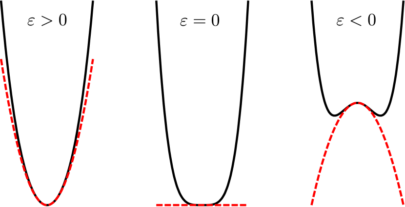
Figure 1: Schematic representation of the potential $V(\phi)=g\phi^{4}/4+\varepsilon\phi^{2}/2$ (solid black line) and its approximation $V(\phi)\approx\varepsilon\phi^{2}/2$ (dashed red line) for three different situations, $\varepsilon>0$ (left), $\varepsilon=\varepsilon_{c}=0$ (middle) and $\varepsilon<0$ (right).

where $\left\langle\textstyle{\ldots}\right\rangle$ denotes the ensemble average, $\beta\equiv(k_{B}T)^{-1}$, $T$ is the temperature and $k_{B}$ is the Boltzmann constant. For $\varepsilon\geq 0$, the field $\phi(x)$, close to the ground state, has small amplitude such that $|g\phi^{3}|\ll|\varepsilon\phi|$. Therefore, to a good approximation, the higher order terms of $\phi$ in $V(\phi)$ can be neglected resulting in $V(\phi)\approx\varepsilon\phi^{2}/2$, as depicted in Fig. 1. Despite of this apparently naive simplification, the linearized stochastic equations of motion still reproduce the dynamics of realistic models Moro:99 ; Chiara:10 ; Nigmatullin:16 . The linearized version of Eq. (4) reads

$$\left(\frac{\partial^{2}}{\partial t^{2}}+\eta\frac{\partial}{\partial t}\right)\phi(x,t)=\left(h^{2}\frac{\partial^{2}}{\partial x^{2}}-\varepsilon(t)\right)\phi(x,t)+\zeta(x,t).$$ (7)

It is convenient to express the field $\phi(x,t)$ in the Fourier space

$$\phi(x,t)=\sum_{n}\varphi_{n}(t)e^{ik_{n}x},$$ (8)

where $k_{n}=2\pi n/L$. For simplicity, we consider periodic boundary conditions, $\phi(0,t)=\phi(L,t)$, and a real field $\phi(x,t)$, which implies $\varphi_{n}(t)=\varphi_{-n}^{*}(t)$. Substituting Eq. (8) in Eq. (7) results in decoupled equations of motion for each mode. The equation for the $n$th mode reads

$$\left(\frac{\partial^{2}}{\partial t^{2}}+\eta\frac{\partial}{\partial t}\right)\varphi_{n}(t)=\left(-k_{n}^{2}h^{2}-\varepsilon(t)\right)\varphi_{n}(t)+\zeta_{n}(t),$$ (9)

with $\langle\zeta_{n}(t)\rangle=0$ and $\langle\zeta_{n}(t)\zeta_{m}(t^{\prime})\rangle=2\eta\beta^{-1}\delta_{nm}\delta(t-t^{\prime})$.

As usual within the framework of statistical mechanics, we are interested in the ensemble averages of observable macroscopic quantities (e.g. correlation length) that are functions of the microstates of the system. The ensemble averaged value $\left<\mathcal{A}[\phi(t),\dot{\phi}(t);t]\right>$ of a physical quantity $\mathcal{A}$ of interest at time $t$ may be obtained by averaging over a number of stochastic trajectories generated by the Langevin dynamics. Typically, the smaller the system, the more stochastic trajectories are necessary to obtain a reliable and meaningful average. Formally, the ensemble average can be obtained by integrating over the field distribution expressed in the Fourier space as

$$\left<\mathcal{A}\right>=\prod\int_{-\infty}^{+\infty}d\varphi_{n}\prod\int_{-\infty}^{+\infty}d\dot{\varphi}_{n}\mathcal{A}\prod P_{n}(t,\varphi_{n},\dot{\varphi}_{n}),$$ (10)

where $P_{n}(t,\varphi_{n},\dot{\varphi}_{n})$ is the time-dependent probability distributions for $n$th mode in the phase space, i.e. it defines the probability of obtaining a value $\varphi_{n}$, and its velocity, $\dot{\varphi}_{n}$, at time $t$ for a mode with momentum $k_{n}=2\pi n/L$. The probability distribution is normalized according to

$$\int_{-\infty}^{+\infty}\int_{-\infty}^{+\infty}d\varphi_{n}d\dot{\varphi}_{n}\,P_{n}(t,\varphi_{n},\dot{\varphi}_{n})=1.$$ (11)

In the Langevin approach, ensemble averaging involves evaluating approximations to these probabilities from the repeated solutions of the stochastic dynamical equations. The Fokker-Planck approach provides an analytic expression for $P_{n}(t,\varphi_{m},\dot{\varphi}_{n})$ as a solution to fully deterministic partial differential equations, as we explain in the following.

Fokker-Planck approach.— The Fokker-Planck formalism is a well-known approach to handle stochastic dynamics, which, in contrast to the Langevin approach focuses from the start on the probability distributions of the stochastic variables. The dynamical equations for the probability distributions are deterministic partial differential equations Risken:84 . The Fokker-Planck counterpart of Eq. (9) that specifies the dynamics of the $n$th mode, reads

$$\frac{\partial P_{n}(t,\varphi_{n},\dot{\varphi_{n}})}{\partial t}=\left[-\frac{\partial}{\partial\varphi_{n}}\dot{\varphi}_{n}+\frac{\partial}{\partial\dot{\varphi}_{n}}\left(\eta\dot{\varphi}_{n}+\right.\right.$$

$$\qquad\left.\left.+\left(h^{2}k_{n}^{2}+\varepsilon(t)\right)\varphi_{n}\right)+\frac{\eta}{\beta}\frac{\partial^{2}}{\partial\dot{\varphi}_{n}^{2}}\right]P_{n}(t,\varphi_{n},\dot{\varphi_{n}}),$$ (12)

which is known as the Kramers equation Risken:84 . Hence the full probabilistic dynamics is acquired solving Eq. (II).

Quantities of interest.— In the spirit of KZ mechanism, we characterize the dynamics by means of the correlations induced in the system as it traverses the second-order phase transition at $\varepsilon_{c}=0$ at different rates $d\varepsilon(t)/dt\propto\tau_{Q}^{-1}$. To quantify such correlations, we introduce the usual two-point correlation function

$$G(x_{1},x_{2},t)=\left\langle\textstyle{\phi(x_{1},t)\phi(x_{2},t)}\right\rangle-\left\langle\textstyle{\phi(x_{1},t)}\right\rangle\left\langle\textstyle{\phi(x_{2},t)}\right\rangle.$$ (13)

As a consequence of the periodic boundary conditions $\phi(0,t)=\phi(L,t)$, the two-point correlation function depends only in the distance $x_{1}-x_{2}$, i.e. $G(x_{1},x_{2},t)\equiv G(x_{1}-x_{2},t)$. The correlation length of the field $\phi(x,t)$ can be defined as

$$\xi_{L}(t)=\frac{\sqrt{\int_{0}^{L/2}dx\,x^{2}\,G(x,t)}}{\sqrt{2\int_{0}^{L/2}dx\,G(x,t)}}.$$ (14)

We also attempt to quantify the defect density formed during the evolution, that is, the number of domains or regions per unit length within $\phi(x,t)$ with an equivalent choice of the broken symmetry. In the defect region the field interpolates rapidly but smoothly between the chosen configurations and thus in those regions the field has large spatial variations. For that reason the density of defects may be quantified by the gradient of the field Laguna:97 . Hence, to quantify such spatial variations, we introduce the density $g_{L}$ as

$$g_{L}(t)=L\frac{\int_{0}^{L}dx\left<\left(\partial_{x}\phi(x,t)\right)^{2}\right>}{\int_{0}^{L}dx\left<\left(\phi(x,t)\right)^{2}\right>}.$$ (15)

The quantities $\xi_{L}(t)$ and $g_{L}(t)$ contain important non-equilibrium dynamical information, allowing us to test the emergence of universal behavior such as KZ scaling.

KZ scaling laws in the thermodynamic limit.— The equilibrium correlation length in the thermodynamic limit diverges as $\xi\propto\left|\varepsilon-\varepsilon_{c}\right|^{-\nu}$, where $\nu$ is the corresponding critical exponent. Additionally, a second-order phase transition is also characterized by a diverging relaxation time, $\tau\propto\left|\varepsilon-\varepsilon_{c}\right|^{-\nu z}$, where $z$ is the dynamical critical exponent Hohenberg:77 . If the fourth and higher order terms of $\phi$ in Eq. (2) are negligible then $\nu=1/2$ (mean field exponent), while depending on the dynamical regime, $z=2$ or $z=1$, for overdamped or underdamped dynamics Laguna:98 ; Chiara:10 . The former regime is found when $\left|\eta\partial_{t}\phi\right|\gg\left|\partial^{2}_{t^{2}}\phi\right|$, while the latter takes place in the opposite limit. To derive scaling laws, we resort to the KZ argument, which states that due to the diverging relaxation time near the critical point, there will be a freeze-out instance, $\hat{t}$, at which the system is not able any longer to adjust its correlation length to its equilibrium value Kibble:76 ; delCampo:14 during the quench. Accordingly, traversing the critical point at a finite rate $\tau_{Q}^{-1}$ provokes the formation of defects or excitations, whose typical size scales as $\hat{\xi}\sim\tau_{Q}^{\nu/(1+z\nu)}$, where $\hat{\xi}$ corresponds to the correlation length at the freeze-out instant. Therefore, the density of excitations will scale as $L^{d}/\hat{\xi}^{d}\sim\tau_{Q}^{-d\nu/(1+z\nu)}$, where $d$ is the dimension of the system. The KZ scaling laws can also be derived using rescaling transformations of the equations of motion Gor:16 , which does not rely on the physical arguments of transition between adiabatic and impulsive dynamics Kibble:76 ; delCampo:14 . In this paper, we show how these rescaling transformations can be applied to our system, elucidating a set of non-equilibrium scaling functions, where KZ scaling laws appear as a special case.

III Overdamped regime: Smoluchowski equation

The general equation of motion which governs the dynamics is given in Eqs. (7) and (II) for Langevin and Fokker-Planck formalism, respectively. However, when the term $\eta\partial_{t}\phi$ dominates, $|\eta\partial_{t}\phi|\gg|\partial^{2}_{t^{2}}\phi|$, the dynamics of $\phi(x,t)$ is overdamped or pure relaxational Hohenberg:77 . In the overdamped regime, the Langevin equation of motion reads

$$\eta\frac{\partial}{\partial t}\phi(x,t)=\left(h^{2}\frac{\partial^{2}}{\partial x^{2}}-\varepsilon(t)\right)\phi(x,t)+\zeta(x,t).$$ (16)

The Fourier decomposition Eq. (8) results in decoupled equations for each of the normal modes. The dynamical equation for the $n$th mode is

$$\eta\frac{\partial}{\partial t}\varphi_{n}(t)=\left(-h^{2}k_{n}^{2}-\varepsilon(t)\right)\varphi_{n}(t)+\zeta_{n}(t),$$ (17)

with $\langle\zeta_{n}(t)\rangle=0$ and $\langle\zeta_{n}(t)\zeta_{m}(t^{\prime})\rangle=2\eta\beta^{-1}\delta_{nm}\delta(t-t^{\prime})$. The Fokker-Planck equation in the overdamped regime is known as the Smoluchowski equation. Let $P_{o,n}(t,\varphi_{n})$ denote the probability distribution for the $n$th mode with $k_{n}=2\pi n/L$; the subscript $o$ emphasizes the overdamped nature of the dynamics. Since $\varphi_{n}(t)$ is in general complex, it is more convenient to express the field as

$$\qquad\phi(x,t)=\frac{\varphi_{0}^{R}(t)}{\sqrt{N_{c}}}$$

$$+\sqrt{\frac{2}{N_{c}}}\sum_{n=1}^{(N_{c}-1)/2}\varphi_{n}^{R}(t)\cos(k_{n}x)+\varphi_{n}^{I}(t)\sin(k_{n}x),$$ (18)

where we have introduced a momentum cut-off $k_{c}$ which sets a maximum number of modes $(N_{c}-1)/2$, and $\varphi_{n}^{R}(t)\equiv\textrm{Re}(\varphi_{n}(t))$ and $\varphi_{n}^{I}(t)\equiv\textrm{Im}(\varphi_{n}(t))$ due to the condition $\varphi_{-n}(t)=\varphi_{n}^{*}(t)$. Note that, without loss of generality, $N_{c}$ is chosen to be odd. Then, the Smoluchowski equation for $P_{o,n}(t,\varphi_{n}^{R,I})$ reads Risken:84

$$\eta\frac{\partial P_{o,n}(t,\varphi_{n}^{R,I})}{\partial t}=\frac{\partial}{\partial\varphi_{n}^{R,I}}\left[\frac{1}{\beta}\frac{\partial}{\partial\varphi_{n}^{R,I}}+\right.$$

$$\qquad+\left.\left(h^{2}k_{n}^{2}+\varepsilon(t)\right)\varphi_{n}^{R,I}\right]P_{o,n}(t,\varphi_{n}^{R,I}).$$ (19)

We will assume that the system is initially in thermal equilibrium at $\varepsilon_{0}$. In thermal equilibrium, a probability distribution, $P^{\rm{th}}_{o,n}$, must fulfill

$$\partial_{t}P^{\rm th}_{o,n}=0.$$ (20)

Substituting Eq. (20) in (III) and solving the resulting differential equation gives

$$P_{o,n}^{\textrm{th}}(\varphi_{n}^{R,I}) =\frac{f_{n}^{\rm th}}{\sqrt{\pi}}e^{-(f_{n}^{\rm th}\varphi_{n}^{R,I})^{2}},$$

$$f_{n}^{\rm th} =\sqrt{\beta\left(h^{2}k_{n}^{2}+\varepsilon_{0}\right)/2}.$$ (21)

As expected, these probabilities correspond to the Boltzmann distribution at given temperature $1/\beta$ of the bath. Note that they exist only for $\varepsilon_{0}>\varepsilon_{c}=0$ as a consequence of the harmonic approximation $V(\phi)\approx\varepsilon\phi^{2}/2$. Having determined the initial state, we now solve Eq. (III) to find the time-dependent probability distribution $P_{o}(t)$. For that, we make use of a Gaussian Ansatz

$$P_{o,n}(t)=\frac{f_{n}(t)}{\sqrt{\pi}}e^{-f_{n}^{2}(t)\varphi_{n}^{2}}.$$ (22)

Substituting Eq. (22) into Eq. (III) gives

$$\frac{\partial}{\partial t}f_{n}(t) =-\frac{2}{{\eta\beta}}f_{n}^{3}(t)+\frac{1}{\eta}\left(h^{2}k_{n}^{2}+\varepsilon(t)\right)f_{n}(t),$$ (23)

with the initial condition determined by the thermal equilibrium, $f_{n}(0)=f_{n}^{\rm th}$. Thus the full knowledge of the probabilistic dynamics is captured in a set of uncoupled differential equations for the variance of each probability distribution.

The knowledge of the functional form of the probability distributions, allows us to explicitly calculate the quantities of interests, namely $\xi_{L}(t)$ and $g_{L}(t)$. Substituting Eq. (22) into the expression for the two-point correlation function given by Eq. (13), and simplifying the resulting expression gives

$$G(x_{1},x_{2},t)=\frac{1}{2N_{c}f_{0}^{2}(t)}+\sum_{n=1}^{N_{c}-1}\frac{\cos(k_{n}(x_{1}-x_{2}))}{N_{c}f_{n}^{2}(t)}.$$ (24)

The correlation length is then obtained using Eq. (14),

$$\xi_{L}(t)=\frac{L}{2\sqrt{6}}\sqrt{1+12f_{0}^{2}(t)\sum_{n=1}^{(N_{c}-1)/2}\frac{(-1)^{n}}{f_{n}^{2}(t)n^{2}\pi^{2}}}.$$ (25)

Similarly, the expression for $g_{L}(t)$ evaluates to

$$g_{L}(t)=L\frac{\sum_{n=1}^{(N_{c}-1)/2}\frac{k_{n}^{2}}{f_{n}^{2}(t)}}{\frac{1}{2f_{0}^{2}(t)}+\sum_{n=1}^{(N_{c}-1)/2}\frac{1}{f_{n}^{2}(t)}}.$$ (26)

Thus, we have obtained analytic expressions for the correlation length and the number of defects as a function of time for non-equilibrium Kibble-Zurek dynamical scenario. In the analytical expressions, we can now look for physical meaning such as the presence of non-equilibrium scaling laws. We break down the discussion into three parts, each of which corresponds to a different quench rate regime: infinitely slow or isothermal quench (the case of thermal equilibrium), sudden quench and finite-rate quench.

Thermal equilibrium.— In the limit $\tau_{Q}\rightarrow\infty$, thermal equilibrium is achieved at any $\varepsilon(t)$. Although this scenario is just a limiting case of a finite-rate quench, it allows us to gather some interesting equilibrium properties which will be helpful later on. We stress that the derived expressions given in Eqs. (25) and (26) are valid for either equilibrium or non-equilibrium. Equilibrium properties are recovered simply by considering thermal probability distributions $P_{o,n}^{\rm th}$ at any $\varepsilon$, that is, $f_{n}^{\rm th}$, given in Eq. (III). In the limit $N_{c}\rightarrow\infty$, the correlation length at thermal equilibrium for finite $L$ reads

$$\xi^{\textrm{th}}_{L}(\varepsilon>0)=\sqrt{\frac{h^{2}}{\varepsilon}-\frac{hL}{2\varepsilon^{1/2}\sinh(\varepsilon^{1/2}L/2h)}},$$ (27)

while in the thermodynamic limit, $L,N_{c}\rightarrow\infty$, keeping the cut-off $k_{c}$ finite, is just $\xi^{\rm th}_{L\rightarrow\infty}(\varepsilon>0)=h\sqrt{1/\varepsilon}$. As we expected for Ginzburg-Landau theory, we obtain a critical exponent $\nu=1/2$ for the diverging correlation length at the critical point, i.e., $\xi\propto|\varepsilon-\varepsilon_{c}|^{-\nu}$. At $\varepsilon=\varepsilon_{c}=0$, the resulting expression is particularly simple for finite $L$,

$$\xi^{\textrm{th}}_{L}(\varepsilon_{c}=0) =\frac{L}{2\sqrt{6}}.$$ (28)

As one expects for a finite system, the correlation length can not exceed the system size, reaching its maximum at the critical point $\xi_{L}\lesssim L$. The previous result gives precisely its saturation value in the harmonic approximation of the Ginzburg-Landau model, as well as the scaling $\xi_{L}(\varepsilon_{c}=0)\propto L$ in agreement with finite-size scaling theory Fisher:72 ; Hohenberg:77 .

In a similar way, we can calculate the $g_{L}^{\textrm{th}}(\varepsilon)$ in the thermodynamic limit as

$$g_{L\rightarrow\infty}^{\rm th}(\varepsilon>0)/L \approx\frac{\int_{0}^{k_{c}}dk\frac{k^{2}}{\beta\left(h^{2}k^{2}+\varepsilon\right)}}{\int_{0}^{k_{c}}dk\frac{1}{\beta\left(h^{2}k^{2}+\varepsilon\right)}}$$

$$=\frac{\varepsilon^{1/2}k_{c}}{h\arctan({hk_{c}\varepsilon^{-1/2}})}-\frac{\varepsilon}{h^{2}},$$ (29)

and hence, as $\varepsilon\rightarrow\varepsilon_{c}=0$, it vanishes as

$$g_{L\rightarrow\infty}^{\rm th}/L\sim\frac{2k_{c}}{h\pi}(\varepsilon-\varepsilon_{c})^{1/2},$$ (30)

revealing its critical exponent, which turns out to be $1/2$.

Sudden quench limit.— We briefly comment on the limit of sudden quenches, that is, when $\tau_{Q}\rightarrow 0$. In this case, as the system has no time to react to external perturbations, the corresponding properties of the system remain unchanged from its initial thermal state. Therefore, the results of sudden quenches are simply given by the thermal initial state at $\varepsilon_{0}$, i.e., $\xi_{L}^{\rm th}(\varepsilon_{0})$ and $g_{L}^{\rm th}(\varepsilon_{0})$, which for the former the expression is explicitly given in Eq. (27).

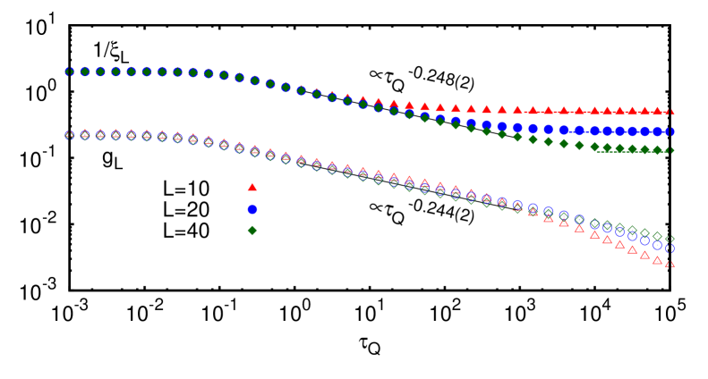
Figure 2: Results for $\xi_{L}$ and $g_{L}$ in the overdamped regime as a function of the quench time $\tau_{Q}$ for three different system sizes, $L=10$, $20$ and $40$ with a fixed cut-off momentum $k_{c}=5\pi$ right at the critical point. Note that, for a better visualization, $g_{L}$ is divided by a $40$. The results clearly show a power-law scaling $\tau_{Q}^{-\nu/(1+z\nu)}=\tau_{Q}^{-1/4}$ for intermediate quench rates as predicted by KZ mechanism. The solid black lines display the fit to a power-law for $L=40$, together with the resulting exponent for both quantities. Dashed lines correspond to the minimum value of $1/\xi_{L}$, i.e., $2\sqrt{6}/L$ for the three different system sizes. Results obtained with $h=5$, $\beta=1$, $\eta=10$, $\varepsilon_{0}=100$ and $\varepsilon_{1}=-10$.

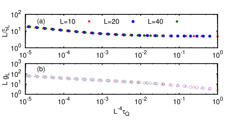
Figure 3: Non-equilibrium finite-size scaling functions in the overdamped regime. The data collapse for different system sizes and quench times for (a) $1/\xi_{L}$ and (b) $g_{L}$ confirm the relation $1/\xi_{L}\sim\tau_{Q}^{-\nu/(1+z\nu)}y_{\xi}(\tau_{Q}L^{-1/\nu-z})$ and $g_{L}\sim\tau_{Q}^{-\nu/(1+z\nu)}y_{g}(\tau_{Q}L^{-1/\nu-z})$, respectively, with $\nu=1/2$ and $z=2$.

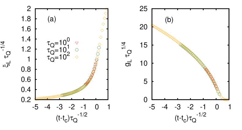
Figure 4: Collapse of (a) $\xi_{L}$ and (b) $g_{L}$ for $L=40$ into a single curve during the whole evolution for the overdamped regime and for different quench times $\tau_{Q}$.

Finite-rate quenches.— We consider now the non-equilibrium dynamics for finite $\tau_{Q}$ in the overdamped regime, where KZ theory predicts scaling laws as a function of the quench rate. That is, we quench linearly the parameter $\varepsilon(t)$ in a time $\tau_{Q}$ according to Eq. (3), and solve the equations of motion (23), by numerical integration. Numerical solutions can be easily done by means of standard Runge-Kutta techniques. We emphasize that solving Eq. (23) immediately allows us to calculate precise average quantities, while the Langevin approach requires evaluating many realizations, which is far more costly from a computational point of view.

We set a momentum cut-off of $k_{N_{c}}=5\pi$, which leads to a maximum number of modes $N_{c}$ for a given length $L$. Initially, the system is prepared in thermal equilibrium at $\varepsilon_{0}=100$ and quenched in a time $\tau_{Q}$ towards $\varepsilon_{1}=-10$. The other parameters are set to $h=5$, $\eta=10$ and $\beta=1$. The results for three different system sizes at $\varepsilon(t)=0$, $L=10$, $20$ and $40$, are presented in Fig. 2, where $g_{L}$ and $1/\xi_{L}$ exhibit KZ scaling at intermediate quench rates. As the system size increases, the region of universal power-law scaling gets broader. For very fast quenches, $\tau_{Q}\rightarrow 0$, $1/\xi_{L}$ and $g_{L}$ saturate to their initial value, while for $\tau_{Q}\rightarrow\infty$, they tend to its value at thermal equilibrium, $g_{L}\rightarrow 0$ and $1/\xi_{L}\rightarrow 2\sqrt{6}/L$, as explained previously. For $L=40$ we perform a fit to obtain the power-law exponent which agrees well with the KZ prediction, $\tau_{Q}^{-\nu/(1+z\nu)}=\tau_{Q}^{-1/4}$ for the overdamped regime. Furthermore, we illustrate the finite-size scaling at intermediate quench rates, which predicts that

$$1/\xi_{L} \sim \tau_{Q}^{-\nu/(1+z\nu)}y_{\xi}(\tau_{Q}L^{-1/\nu-z})$$ (31)

$$g_{L} \sim \tau_{Q}^{-\nu/(1+z\nu)}y_{g}(\tau_{Q}L^{-1/\nu-z}),$$ (32)

where $y_{\xi}(x)$ and $y_{g}(x)$ are non-equilibrium scaling functions which fulfill $y(x\ll 1)\sim$ constant (where KZ scaling law emerges) and $y(x\gg 1)\sim x^{\nu/(1+z\nu)}$, for nearly adiabatic quenches Nigmatullin:16 . For that, we plot $L/\xi_{L}$ which is expected to follow a functional form $L\tau_{Q}^{-\nu/(1+z\nu)}y_{\xi}(\tau_{Q}L^{-1/\nu-z})$ or simply $x^{-\nu/(1+z\nu)}y_{\xi}(x)$ being $x=\tau_{Q}L^{-1/\nu-z}$. Thus, $L/\xi_{L}$ and $g_{L}L$ depend only on the scaling variable $\tau_{Q}L^{-1/\nu-z}$. The collapse of the data onto a single curve shown in Fig. 3 confirms this non-equilibrium scaling hypothesis.

Additionally, we demonstrate the universality of the phase transition dynamics by transforming physical quantities in such a way that any $\tau_{Q}$-dependence is removed from the equations of motion, following the theory developed in Gor:16 . This is achieved by performing transformations $x\rightarrow x\tau_{Q}^{-1/4}$ and $t\rightarrow(t-t_{c})\tau_{Q}^{-1/2}$, where $t_{c}=\tau_{Q}\frac{\varepsilon_{0}}{\varepsilon_{0}-\varepsilon_{1}}$ is the instance at which the critical point is crossed. In this rescaled frame the dynamics is universal and hence the functional dependence of $\xi_{L}\tau_{Q}^{-1/4}$ and $g_{L}\tau_{Q}^{1/4}$ on $(t-t_{c})\tau_{Q}^{-1/2}$ is expected to be the same irrespective of the value of $\tau_{Q}$. This universality during the whole evolution is demonstrated in Fig. 4, which shows the collapse of the results for three different values of $\tau_{Q}$ onto two curves, one for $\xi_{L}$ and one for $g_{L}$.

IV General and underdamped regime: Kramers equation

Let us recall that the Kramers equation Eq. (II) describes the general dynamical regime that includes both dissipative and inertial terms. In our particular case, the Fokker-Planck equation which describes the dynamics reads

$$\frac{\partial P_{n}(t,\varphi_{n},\dot{\varphi}_{n})}{\partial t}=\left[-\frac{\partial}{\partial\varphi_{n}}\dot{\varphi}_{n}+\frac{\partial}{\partial\dot{\varphi}_{n}}\left(\eta\dot{\varphi}_{n}+\right.\right.$$

$$\qquad\left.\left.+\left(h^{2}k_{n}^{2}+\varepsilon(t)\right)\varphi_{n}\right)+\frac{\eta}{\beta}\frac{\partial^{2}}{\partial\dot{\varphi}_{n}^{2}}\right]P_{n}(t,\varphi_{n},\dot{\varphi}_{n}),$$ (33)

where $P_{n}(t,\varphi_{n}(t),\dot{\varphi}_{n}(t))$ is now a two-dimensional probability distribution at time $t$. The analysis of Eq. (IV) is more intricate, but nevertheless the procedure is similar to the one presented in Sec. III for the overdamped dynamics.

Thermal equilibrium states are obtained from $\partial_{t}P_{n}^{\textrm{th}}=0$, whose solution in terms of $\varphi_{n}^{R}\equiv{\rm Re}(\varphi_{n})$ and $\varphi_{n}^{I}\equiv{\rm Im}(\varphi_{n})$ reads

$$P_{n}^{\textrm{th}} =\frac{\sqrt{(A_{n}^{\textrm{th}}B_{n}^{\textrm{th}})^{2}-(C_{n}^{\textrm{th}})^{2}}}{2\pi}\,\times$$

$$\times\textrm{Exp} \left[-\frac{1}{2}\left(\left(A_{n}^{\textrm{th}}\varphi_{n}^{R,I}\right)^{2}+\left(B_{n}^{\textrm{th}}\dot{\varphi}_{n}^{R,I}\right)^{2}-2C_{n}^{\textrm{th}}\varphi_{n}^{R,I}\dot{\varphi}_{n}^{R,I}\right)\right]$$ (34)

where

$$A_{n}^{\textrm{th}} =\sqrt{\beta\left(h^{2}k_{n}^{2}+\varepsilon\right)},$$ (35)

$$B_{n}^{\textrm{th}} =\sqrt{\beta},$$ (36)

$$C_{n}^{\textrm{th}} =0.$$ (37)

The time evolution of the probability distributions $P_{n}(t)$ is given by time-dependent coefficients $A_{n}(t)$, $B_{n}(t)$ and $C_{n}(t)$. In this way, three coupled differential equations per mode under the protocol $\varepsilon(t)$ determine the dynamics,

$$\frac{\partial A_{n}(t)}{\partial t} =-\frac{C_{n}(t)}{A_{n}(t)}\left(\varepsilon(t)+h^{2}k_{n}^{2}+\frac{\eta C_{n}(t)}{\beta}\right),$$ (38)

$$\frac{\partial B_{n}(t)}{\partial t} =\eta B_{n}(t)-\frac{\eta}{\beta}B_{n}^{3}(t)+\frac{C_{n}(t)}{B_{n}(t)},$$ (39)

$$\frac{\partial C_{n}(t)}{\partial t} =A_{n}^{2}(t)+\eta C_{n}(t)-B_{n}^{2}(t)\left(h^{2}k_{n}^{2}+\right.$$

$$\hskip 85.35826pt\left.+\varepsilon(t)+\frac{2\eta C_{n}(t)}{\beta}\right).$$ (40)

The average quantities are obtained in the same way as in the overdamped regime, but with the time-dependent probability distributions also dependent on $\dot{\varphi}_{n}$. Indeed, we can define the probability distribution $Q_{n}(t,\varphi_{n}^{R,I})$ once the velocity dependence is integrated out,

$$Q_{n}(t,\varphi_{n}^{R,I}) =\int_{-\infty}^{+\infty}d\dot{\varphi}_{n}^{R,I}\,P_{n}(t,\varphi_{n}^{R,I},\dot{\varphi}_{n}^{R,I})$$

$$=\frac{F_{n}(t)}{\sqrt{\pi}}e^{-F_{n}^{2}(t)(\varphi_{n}^{R,I})^{2}},$$ (41)

where $F_{n}(t)$ depends on the coefficients $A_{n}(t)$, $B_{n}(t)$ and $C_{n}(t)$ as

$$F_{n}(t) =\sqrt{\frac{1}{2B_{n}^{2}(t)}\left(A_{n}^{2}(t)B_{n}^{2}(t)-C_{n}^{2}(t)\right)}.$$ (42)

This allows us to directly apply the same expressions as those derived for the overdamped regime. Eqs. (25) and (26) for correlation length $\xi_{L}(t)$ and density $g_{L}(t)$ can be directly applied by just replacing $f_{n}(t)$ with $F_{n}(t)$.

Thermal equilibrium and sudden quenches.— Clearly, thermal equilibrium does not depend on the considered dynamical regime. Therefore, the same thermal equilibrium probability distributions are retrieved from Eq. (IV) and we refer to Sec. III for the discussion on equilibrium features, as well as the opposite limit, $\tau_{Q}\rightarrow 0$, of sudden quenches.

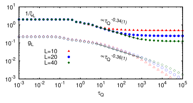
Figure 5: Results for $\xi_{L}$ and $g_{L}$ in the underdamped regime ($\eta=0.1$) as a function of the quench time $\tau_{Q}$ for three different system sizes, $L=10$, $20$ and $40$ with a fixed cut-off momentum $k_{c}=5\pi$ right at the critical point. Note that $g_{L}$ is divided by $40$ for a better visualization. The results clearly show a power-law scaling $\tau_{Q}^{-\nu/(1+z\nu)}=\tau_{Q}^{-1/3}$ for intermediate quench rates as predicted by the theory. The solid black lines display the fit to a power-law for $L=40$, together with the resulting exponent. Dashed lines correspond to the minimum value of $1/\xi_{L}$, i.e., $2\sqrt{6}/L$ for the three different system sizes. Results were obtained with $h=5$, $\beta=1$, $\varepsilon_{0}=100$ and $\varepsilon_{1}=-10$.

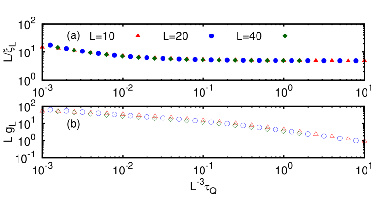
Figure 6: Non-equilibrium finite-size scaling functions in the underdamped regime ($\eta=0.1$) for different system sizes a quench times. The data collapse for (a) $1/\xi_{L}$ and (b) $g_{L}$ confirm the relation $1/\xi_{L}\sim\tau_{Q}^{-\nu/(1+z\nu)}y_{\xi}(\tau_{Q}L^{-1/\nu-z})$ and $g_{L}\sim\tau_{Q}^{-\nu/(1+z\nu)}y_{g}(\tau_{Q}L^{-1/\nu-z})$, respectively, being the critical exponents in the underdamped case $\nu=1/2$ and $z=1$.

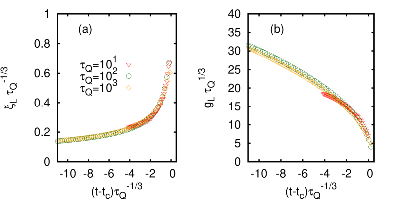
Figure 7: Collapse of (a) $\xi_{L}$ and (b) $g_{L}$ for $L=40$ into a single curve during the whole evolution for the underdamped regime and for different quench times $\tau_{Q}$.

Finite-rate quenches.— As in the case of overdamped dynamics, the KZ scaling laws are observed at finite quench rates. We solve numerically the equations of motion Eq. (38) to obtain the time-dependent probability distributions for different $\tau_{Q}$. Then, from $F_{n}(t)$ we calculate $\xi_{L}(t)$ and $g_{L}(t)$ using Eqs. (25) and (26), respectively. As in the overdamped regime, we set a momentum cut-off of $k_{c}=5\pi$. The initial thermal state at $\varepsilon_{0}=100$ is quenched in a time $\tau_{Q}$ towards $\varepsilon_{1}=-10$. Additionally, we set $h=5$ and $\beta=1$. To illustrate the KZ scaling in the underdamped regime, we select a small friction coefficient $\eta=0.1$. The results are presented in Fig. 5 for three different system sizes, $L=10$, $20$ and $40$, where the latter already exhibits a power-law scaling $\sim\tau_{Q}^{\alpha}$ for wide range of quench times. The performed fit gives an exponent $\alpha=-0.34(1)$ for $1/\xi_{L}$, in agreement with the predicted KZ scaling $\tau_{Q}^{-\nu/(1+z\nu)}=\tau_{Q}^{-1/3}$ since $\nu=1/2$ and $z=1$. A more pronounced deviation is found for $g_{L}$, with $\alpha=-0.36(1)$, which might be caused by finite-size effects. Moreover, in Fig. 6 the finite-size scaling at intermediate quench rates is verified. The data collapse onto a single curve corroborates the relations $1/\xi_{L}\sim\tau_{Q}^{-\nu/(1+z\nu)}y_{\xi}(\tau_{Q}L^{-1/\nu-z})$ and $g_{L}\sim\tau_{Q}^{-\nu/(1+z\nu)}y_{g}(\tau_{Q}L^{-1/\nu-z})$. Recall that $L/\xi_{L}$ and $Lg_{L}$ are expected to follow $x^{-\nu/(1+z\nu)}y_{\xi}(x)$ and $x^{-\nu/(1+z\nu)}y_{g}(x)$ where $x=\tau_{Q}L^{-1/\nu-z}$ is a scaling variable and $y(x)$ are non-equilibrium scaling functions.

Finally, we exemplify the universality of the dynamics in the underdamped regime. If $\left|\eta\partial_{t}\phi\right|\ll\left|\partial^{2}_{t^{2}}\phi\right|$, one removes the $\tau_{Q}$ dependence by performing the transformation $x\rightarrow x\tau_{Q}^{-1/3}$ and $t\rightarrow(t-t_{c})\tau_{Q}^{-1/3}$ Gor:16 . Note that the transformation is different to the overdamped case. The quantities $\xi_{L}\tau_{Q}^{-1/3}$ and $g_{L}\tau_{Q}^{1/3}$ are expected to collapse for different quench times $\tau_{Q}$ when plotted against the rescaled time $(t-t_{c})\tau_{Q}^{-1/3}$. This collapse is shown in Fig. 7, where we plot the results of the calculations of $\xi_{L}(t)$ and $g_{L}(t)$ for three different values of $\tau_{Q}$ in the rescaled coordinates.

V Coulomb crystals: linear to zigzag phase transition

The analysis in the previous sections has been done for phase transitions described by a one-dimensional Ginzburg-Landau field theory. However, the Fokker-Planck approach is valid beyond the Ginzburg-Landau theory; the knowledge of the quench function and the dispersion relation of the system is sufficient to predict the expected density of defects or any other statistical observable. We will illustrate this by applying our method to the problem of dynamic structural phase transition in Coulomb crystals Fishman:08 ; Chiara:10 .

Coulomb crystals are ordered structures that form when charged particles in a global confining potential are cooled below a critical temperature. An example of the physical realization of Coulomb crystals are ion crystals in Paul traps. Structural transitions in Coulomb crystal can be induced by varying the global confining potential Retzker:08 ; Partner:15 . The KZ mechanism of defect formation was studied numerically and experimentally using linear to zigzag non-equilibrium phase transition in ion traps Pyka:13 ; Ulm:13 . The analysis in references delCampo:10 ; Chiara:10 ; Nigmatullin:16 relied on the mapping of the linear to zigzag transition to a Ginzburg-Landau field theory model. In this section, we show how to use the methods developed in this paper to analyze the dynamic linear to zigzag transition without resorting to Ginzburg-Landau theory.

We consider $N$ charged particles moving in a periodic cell of size $L$. The periodic boundary conditions simplify the analysis since they result in a homogeneous Coulomb crystal. Moreover, periodic boundary condition can be realized with the existing technology of ring ion traps Wang:15 ; Li:16 . The potential energy of the $N$ particles reads

$$V=\frac{1}{2}\sum_{j=1}^{N}m\omega_{t}^{2}z_{j}^{2}+\frac{1}{2}\sum_{j=1}^{N}\sum_{j\neq i}\frac{Q^{2}}{|\textbf{r}_{i}-\textbf{r}_{j}|},$$ (43)

where $\textbf{r}_{i}=(x_{j},z_{j})$ is the coordinate of the $j$th ion, $m$ is the mass of the ions, $\omega_{t}$ is the transverse trapping secular frequency and $Q^{2}\equiv e^{2}/4\pi\epsilon_{0}$. There exists a critical frequency value $\omega_{t}^{c}=\sqrt{7\zeta_{R}(3)/2}\omega_{0}$, where $\omega_{0}=\sqrt{Q^{2}/ma^{3}}$ and $\zeta_{R}(x)$ is the Riemann zeta function. For $\omega_{t}>\omega_{t}^{c}$ the lowest energy configuration is a linear chain and for $\omega_{t}<\omega_{t}^{c}$ the lowest energy configuration is a two-row zigzag chain.

Initially, the $N$ ions are in thermal equilibrium in a linear chain configuration. The transverse frequency $\omega_{t}$ is then quenched linearly in time through the critical point $\omega_{t}^{c}$, thereby inducing a transition from a linear to zigzag configuration at a rate proportional to $1/\tau_{Q}$

$$\omega_{t}(t)=\begin{cases}\omega_{i}&\quad\textrm{for }t<0\\ \omega_{i}+\frac{\omega_{f}-\omega_{i}}{\tau_{Q}}t&\quad\textrm{for }0\leq t<\tau_{Q}\\ \omega_{f}&\quad\textrm{for t}\geq\tau_{Q},\end{cases}$$ (44)

where $\omega_{i}>\omega_{t}^{c}$ and $\omega_{f}<\omega_{t}^{c}$. Since the quench is performed at finite rate, the system is driven out of equilibrium and there is a non-zero probability of formation of a number of structural defects.

Langevin approach.— The expectation of any observable $\left\langle\mathcal{A}(t)\right\rangle$ (including the number of defects) can be evaluated by repeatedly solving the stochastic equations of motion that describe the dynamics of the systems, and then estimating the expectation from the obtained sample of trajectories. The dynamics of the system is determined by the following Langevin equations of motion

$$m\frac{d^{2}x_{j}}{dt^{2}}+\eta\frac{dx_{j}}{dt}+\frac{\partial V}{\partial x_{j}} = \zeta_{j}^{x}(t),$$ (45)

$$m\frac{d^{2}z_{j}}{dt^{2}}+\eta\frac{dz_{j}}{dt}+\frac{\partial V}{\partial z_{j}} = \zeta_{j}^{z}(t).$$ (46)

There, $\eta$ is the friction coefficient and $\zeta_{j}^{x,z}$ is the stochastic force that satisfies the following statistical relations

$$\left\langle\zeta_{j}^{\alpha}(t)\right\rangle = 0,$$ (47)

$$\left\langle\zeta_{j}^{\alpha}(t)\zeta_{k}^{\gamma}(t^{\prime})\right\rangle = 2\eta\beta^{-1}\delta_{\alpha\gamma}\delta_{jk}\delta(t-t^{\prime}),$$ (48)

where $\alpha,\gamma\in\{x,z\}$ and $j,k\in\{1,2,...,N\}$.

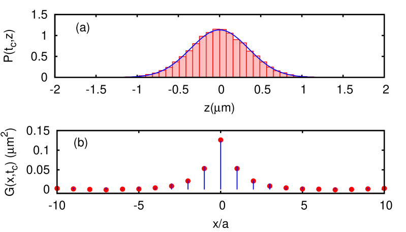
Figure 8: (a) Probability distribution for the transverse displacement $z$ and (b) two-point correlation function $G(x,t)$ at the critical point for a quench of $\tau_{Q}=41.7\ \mu$s and $N=21$ ions. The histogram and points correspond to the Langevin approach, averaging over $2000$ stochastic trajectories, while solid lines to the Fokker-Planck approach. See main text for further details regarding the used parameters.

We solve equations of motion, Eqs. (45)-(46), using the Langevin Impulse integration method with a timestep of $10$ ns Skeel:02 . We consider a system of $N=21$ ions, with inter-ion spacing in the linear configuration $a=10\ \mu$m, mass $m=172$ amu, which corresponds to $\textrm{Yb}^{+}$ ions, temperature $T=5$ mK and friction coefficient $\eta=1.5\times 10^{-21}$ kg s^-1 Pyka:13 . The initial and final transverse frequency is set to $\omega_{i}=2\pi\times 477.5$ kHz and $\omega_{f}=2\pi\times 159$ kHz. Note that $\omega_{0}=2\pi\times 143$ kHz and hence, the critical frequency is $\omega_{t}^{c}=2\pi\times 293.4$ kHz. To ensure that the system is initially in thermal equilibrium, the system is evolved under fixed trap parameters for $100\ \mu$s before starting the quench protocol. The quench time $\tau_{Q}$ is varied from $10\ \mu$s to $400\ \mu$s. For each value of $\tau_{Q}$, we perform $2000$ simulations in order to obtain accurate estimations of statistical observables such as two-point correlation function $G(x,t)$, correlation length $\xi(t)$, number of defects at the end of the quench $\left<N_{d}\right>$, and probability distributions of the transverse displacement $z(t)$, which due to translational symmetry does not depend on the ion position.

Fig. 8 shows an example of the results of the calculations for a selected quench time $\tau_{Q}=41.7\ \mu$s, namely the probability distribution of the transverse displacement and the two-point correlation function at the critical point. In Fig. 9, we plot the scaling of several quantities as a function of the quench time $\tau_{Q}$. These quantities are the correlation length $\xi$ and the averaged square displacement $\left<z^{2}\right>$ at $\omega_{t}(t_{c})=\omega_{t}^{c}$, and the number of defects $\left<N_{d}\right>$ at the end of the quench. We find that the scaling exponent is $\sim 1/3$, which is in agreement with the existing results in Refs. Chiara:10 ; Nigmatullin:16 , which predict this scaling by mapping the problem to GL theory and using the KZ relation $\tau_{Q}^{-\nu/(1+z\nu)}$ with $\nu=1/2$ and $z=1$. Furthermore, following the theory developed in Gor:16 , we can transform physical quantities to remove their dependence on the quench time $\tau_{Q}$, as explained and demonstrated in previous sections for GL theory. This entails the collapse of the correlation length $\xi$ into a single curve for different $\tau_{Q}$ values when $\xi\tau_{Q}^{-1/3}$ is plotted against the rescaled time $(t-t_{c})\tau_{Q}^{-1/3}$ with $\omega_{t}(t_{c})=\omega_{t}^{c}$, as shown in Fig. 10. Note that since $\nu=1/2$ and $z=1$, the used transformation to obtain the collapse is equivalent as GL theory in underdamped regime (see Sec. IV). In addition to the results of the Langevin dynamics simulations, Figs. 8, 9 and 10 include the results of the Fokker-Planck approach. The results show a good agreement with the Fokker-Planck description of the problem even when non-linear terms are neglected, as we explain in the following.

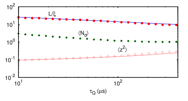
Figure 9: Scaling of correlation length $L/\xi$, mean square transverse displacement $\left<z^{2}\right>$ at the critical point, using Langevin approach, averaging over $2000$ stochastic trajectories (points) and Fokker-Planck formalism (solid lines), together with the average number of structural defects $\left<N_{d}\right>$ at the end of the quench, which saturates to $1$ for slow quenches. Note that $L/\xi\sim 10\left<N_{d}\right>$. A fit to a $\tau_{Q}^{\alpha}$ gives $\alpha=-0.31(1)$ and $-0.30(1)$ in the range of $\tau_{Q}\in\left[40,200\right]\ \mu$s for $L/\xi$ and $\left<N_{d}\right>$ using Langevin approach, respectively, while for Fokker-Planck results in $-0.29(1)$ for $L/\xi$.

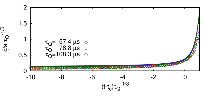
Figure 10: Collapse of $\xi$ into a single curve for $N=21$ ions evolving towards the critical point for three different quench times $\tau_{Q}$. Note that $t_{c}$ corresponds to the time at which the critical frequency is reached, i.e., $\omega_{t}(t_{c})=\omega_{t}^{c}$. The points correspond to the Langevin approach, averaging over $2000$ stochastic trajectories, while solid lines to the Fokker-Planck approach.

Fokker-Planck approach.— We now apply the Fokker-Planck approach to the problem of non-equilibrium quenches from the linear to zigzag configuration. At the start of the quench the system is in the symmetric linear phase. The equilibrium configuration of the ions is given by $\textbf{r}_{j}^{(0)}=(x_{j}^{(0)},0)$, where for convenience we take $x_{i}>x_{j}$ for $i>j$. Due to the periodic boundary conditions, the equilibrium inter-particle distance is constant i.e. $a=x_{j+1}^{(0)}-x_{j}^{(0)}$. The linearized equations of motions for small displacements around the equilibrium configurations $q_{j}=x_{j}-x_{j}^{(0)}$ and $z_{j}$ are obtained by Taylor expanding the potential. In the second-order Taylor expansion the axial and transverse motion decouple Chiara:10 . The equations of motion for the transverse displacements in this limit are

$$m\ddot{z}_{j}+\eta\dot{z}_{j}+m\omega_{t}^{2}z_{j}-\frac{1}{2}\sum_{i\neq j}\mathcal{K}_{i,j}\left(z_{j}-z_{i}\right)=\zeta_{j}^{z}(t)$$ (49)

where $\mathcal{K}_{i,j}\equiv\left.-\partial^{2}V/\partial x_{j}\partial x_{i}\right|_{x_{j}^{(0)}}$ is given by

$$\mathcal{K}_{i,j}=\frac{2Q^{2}}{\left|x_{i}^{(0)}-x_{j}^{(0)}\right|^{3}}.$$ (50)

Eq. (49) describes the motion of coupled oscillators, which can be decoupled by rewriting it in terms of the normal modes. The relation between the transverse coordinate vector $\vec{z}$ and the normal mode vector $\vec{\Psi}$ can be written as

$$z_{j}=\frac{1}{\sqrt{N}}\Psi_{0}^{+}+$$

$$+\sqrt{\frac{2}{N}}\sum_{n=1}^{(N-1)/2}\left(\Psi_{n}^{+}\cos(k_{n}ja)+\Psi_{n}^{-}\sin(k_{n}ja)\right),$$ (51)

where $k_{n}=2\pi n/Na$ and the sign $+$ ($-$) indicates the parity under $k_{n}\rightarrow-k_{n}$. Substituting Eq. (51) in (49) gives

$$m\ddot{\Psi}^{\pm}_{n}+\eta\dot{\Psi}^{\pm}_{n}+m\mbox{$\omega$}_{n}^{2}(t)\Psi_{n}^{\pm}=\zeta_{n}^{\pm}(t),$$ (52)

where $\omega_{n}(t)$ defines the frequency of the normal modes,

$$\omega_{n}^{2}(t)=\omega_{t}^{2}(t)-2\left(\frac{2Q^{2}}{ma^{3}}\right)\sum_{j=1}^{N}\frac{1}{j^{3}}\sin^{2}\left(\frac{k_{n}ja}{2}\right),$$ (53)

and $\zeta_{n}^{\pm}(t)$ represents the stochastic force in the normal mode space, which again fulfills $\left<\zeta_{n}^{p}(t)\zeta_{m}^{q}(t^{\prime})\right>=2\eta/\beta\delta_{pq}\delta_{nm}\delta(t-t^{\prime})$. The Fokker-Planck equations corresponding to the Langevin Eq. (52) are

$$\frac{\partial P_{n}(t,\Psi_{n},\dot{\Psi}_{n})}{\partial t}=\left[-\frac{\partial}{\partial\Psi_{n}}\dot{\Psi}_{n}+\frac{\eta}{2\beta m^{2}}\frac{\partial^{2}}{\partial\dot{\Psi}_{n}^{2}}+\right.$$

$$+\left.\frac{\partial}{\partial\dot{\Psi}_{n}}\left(\frac{\eta}{m}\dot{\Psi}_{n}+\omega_{n}^{2}(t)\Psi_{n}\right)\right]P_{n}(t,\Psi_{n},\dot{\Psi}_{n}).$$ (54)

Therefore, we have reduced the problem to the solution of $N$ deterministic Fokker-Planck equations that determine the mode population probabilities at a chosen time $t$. Using Eq. (54) and the expressions for $P_{n}$, following the same procedure as in Sec. IV, allows the determination of any statistical observable, as well for example, the probability distributions for $z_{j}$ at time $t$. Note that, from Eq. (51) and since $\Psi_{n}^{\pm}$ are statistically independent and Gaussian distributed, $P(t,z_{j})$ adopts also a Gaussian form and independent of $j$,

$$P(t,z)=\frac{1}{\sqrt{2\pi\sigma^{2}(t)}}e^{-z^{2}/(2\sigma^{2}(t))},$$ (55)

with a time-dependent variance

$$\sigma^{2}(t)=\frac{1}{N}\left(\frac{1}{2F_{0}^{2}(t)}+\sum_{n=1}^{(N-1)/2}\frac{1}{F_{n}^{2}(t)}\right),$$ (56)

where $F_{n}(t)$ is obtained from Eq. (54) in the same way as explained in Sec. IV. In particular, we calculate the non-equilibrium correlation length $\xi$ and the mean square transverse displacement $\left<z^{2}\right>$ for the same set of parameters as was used previously in the Langevin approach. A comparison between the two approaches is shown in Fig. 8 and 9. We emphasize that the Fokker-Planck results which have been obtained under a simplified description of the realistic model, where non-linear terms and fluctuations in the longitudinal coordinates have been neglected, still reproduce essential features of the considered non-equilibrium scenario in a quantitative way.

VI Conclusions

We have studied the emergence of universal scaling laws in non-equilibrium second-order phase transitions using Fokker-Planck formalism. We verify that the developed approach reproduces Kibble-Zurek scaling laws in one dimensional Ginzburg-Landau model in overdamped and underdamped dynamical regimes. Additionally, we use this approach to obtain the universal finite-size scaling functions and demonstrate the universality of the dynamics.

There are several advantages of the developed method. It allows us to determine universal scaling laws in a efficient way in comparison to Langevin approach, where ensemble averages must be computed numerically. It provides analytic results that are easily amenable to further analysis. Moreover, it has an extended range of applicability - it can be used to derive insights into the non-equilibrium symmetry breaking phase transitions in overdamped, underdamped and intermediate dynamical regimes; finite as well as infinite systems and systems that are not described directly by the Ginzburg-Landau model. We have illustrated the power of the developed framework by analyzing the non-equilibrium linear to zigzag structural phase transition of an ion chain with periodic boundary conditions. We find an excellent agreement between the results obtained using the Fokker-Planck approach and the non-linear Langevin dynamics simulations.

One challenge for future theoretical work is to include the coupling between the normal modes of the system during quench protocol and find a way to predict the resulting corrections to the scaling laws. Another interesting direction of research would be apply this framework to investigation of scaling laws of other important quantities in stochastic thermodynamics such as entropy production and work done.

- (1) L. D. Landau, and E. M. Lifshitz, Statistical Physics, (Butterworth–Heinemann, Vol. 5 3rd Ed., 1980).
- (2) T. W. B. Kibble, J. Phys. A: Math. Gen. 9, 1387 (1976); W. H. Zurek, Nature 317, 505 (1985); T. Kibble, Physics Today 60, 47 (2007).
- (3) A. del Campo, and W. H. Zurek, Int. J. Mod. Phys. A 29, 1430018 (2014).
- (4) L. E. Sadler, J. M. Higbie, S. R. Leslie, M. Vengalattore, and D. M. Stamper-Kurn, Nature (London) 443, 312 (2006).
- (5) C. N. Weiler, T. W. Neely, D. R. Scherer, A. S. Bradley, M. J. Davis, and B. P. Anderson, Nature (London) 455, 948 (2008).
- (6) G. Lamporesi, S. Donadello, S. Serafini, F. Dalfovo, and G. Ferrari, Nat. Phys. 9, 656 (2013).
- (7) K. Pyka, J. Keller, H. L. Partner, R. Nigmatullin, T. Burgermeister, D. M. Meier, K. Kuhlmann, A. Retzker, M. B. Plenio, W. H. Zurek, A. del Campo, and T. E. Mehlstäubler, Nat. Commun. 4, 2291 (2013).
- (8) S. Ulm, J. Rossnagel, G. Jacob, C. Degünther, S. T. Dawkins, U. G. Poschinger, R. Nigmatullin, A. Retzker, M. B. Plenio, F. Schmidt-Kaler, and K. Singer, Nat. Commun. 4, 2290 (2013).
- (9) H. Risken, The Fokker-Planck equation: methods of solution and applications (Springer-Verlag, New-York, 1984).
- (10) R. Nigmatullin, A. del Campo, G. De Chiara, G. Morigi, M. B. Plenio, and A. Retzker, Phys. Rev. B, 93, 014106 (2016).
- (11) G. De Chiara, A. del Campo, G. Morigi, M. B. Plenio, and A. Retzker, New J. Phys. 12, 115003 (2010).
- (12) P. C. Hohenberg, and B. I. Halperin, Rev. Mod. Phys. 49, 435 (1977).
- (13) E. Moro, and G. Lythe, Phys. Rev. E 59, R1303(R) (1999).
- (14) P. Laguna, and W. H. Zurek, Phys. Rev. Lett. 78, 2519 (1997).
- (15) P. Laguna, and W. H. Zurek, Phys. Rev. D 58, 085021 (1998).
- (16) G. Nikoghosyan, R. Nigmatullin, and M. B. Plenio, Phys. Rev. Lett. 116, 080601 (2016).
- (17) M. E. Fisher, and M. N. Barber, Phys. Rev. Lett. 28, 1516 (1972).
- (18) S. Fishman, G. De Chiara, T. Calarco, and G. Morigi, Phys. Rev. B 77, 064111 (2008).
- (19) A. Retzker, R.C. Thompson, D.M. Segal, and M.B. Plenio, Phys. Rev. Lett. 101, 260504 (2008).
- (20) H.L. Partner, A. del Campo, W.H. Zurek, A. Retzker, M. B. Plenio, Karsten Pyka, J. Keller, T. Burgermeister, R. Nigmatullin and T. E. Mehlstäubler, Physica B 460, 114 (2015).
- (21) A. del Campo, G. De Chiara, G. Morigi, M. B. Plenio, and A. Retzker, Phys. Rev. Lett. 105, 075701 (2010).
- (22) P.-J. Wang, T. Li, C. Noel, A. Chuang, X. Zhang, and H. Häffner, J. Phys. B: At. Mol. Opt. Phys. 48 205002 (2015).
- (23) H.-K. Li, E. Urban, C. Noel, A. Chuang, Y. Xia, A. Ransford, B. Hemmerling, Y. Wang, T. Li, H. Häffner, X. Zhang arxiv:1605.02143
- (24) R. D. Skeel, and J. S. A. Izaguirre, Mol. Phys. 100, 3885 (2002).