Antinucleon-nucleon interaction at next-to-next-to-next-to-leading order
in chiral effective field theory

Abstract

Results for the antinucleon-nucleon ($\bar{N}N$) interaction obtained at next-to-next-to-next-to-leading order in chiral effective field theory (EFT) are reported. A new local regularization scheme is used for the pion-exchange contributions that has been recently suggested and applied in a pertinent study of the $NN$ force within chiral EFT. Furthermore, an alternative strategy for estimating the uncertainty is utilized that no longer depends on a variation of the cutoffs. The low-energy constants associated with the arising contact terms are fixed by a fit to the phase shifts and inelasticities provided by a phase-shift analysis of $\bar{p}p$ scattering data. An excellent description of the $\bar{N}N$ amplitudes is achieved at the highest order considered. Moreover, because of the quantitative reproduction of partial waves up to $J=3$, there is also a nice agreement on the level of $\bar{p}p$ observables. Specifically, total and integrated elastic and charge-exchange cross sections agree well with the results from the partial-wave analysis up to laboratory energies of $300$ MeV, while differential cross sections and analyzing powers are described quantitatively up to $200$-$250$ MeV. The low-energy structure of the $\bar{N}N$ amplitudes is also considered and compared to data from antiprotonic hydrogen.

1 Introduction

The Low Energy Antiproton Ring (LEAR) at CERN has provided a wealth of data on antiproton-proton ($\bar{p}p$) scattering [1, 2, 3] and triggered a great number of pertinent investigations [4, 5, 6, 7, 8, 9, 10, 11]. Its closure in 1996 has led to a noticeable quiescence in the field of low-energy antiproton physics. However, over the last decade there has been a renewed interest in antinucleon-nucleon ($\bar{N}N$) scattering phenomena, prompted for the main part by measurements of the $\bar{p}p$ invariant mass in the decays of heavy mesons such as $J/\psi$, $\psi^{\prime}$, and $B$, and of the reaction cross section for $e^{+}e^{-}\to\bar{p}p$. In several of those reactions a near-threshold enhancement in the mass spectrum was found [12, 13, 14, 15]. While those observations nourished speculations about new resonances, $\bar{p}p$ bound states, or even more exotic objects in some parts of the physics community, others noted that such data could provide a unique opportunity to test the $\bar{p}p$ interaction at very low energies [16, 17, 18, 19, 20, 21, 22, 23, 24, 25, 26, 27, 28]. Indeed, in the aforementioned decays one has access to information on $\bar{p}p$ scattering at significantly lower energies than it was ever possible at LEAR. In the future one expects a further boost of activities related to the $\bar{N}N$ interaction due to the Facility for Antiproton and Ion Research (FAIR) in Darmstadt whose construction is finally on its way [29]. In the course of this renewed interest new phenomenological $\bar{N}N$ potential models have been published [30, 31]. Moreover, an update of the Nijmegen partial-wave analysis (PWA) of antiproton-proton scattering data [10] has been presented [32].

Over the same time period another important developement took place, namely the emergence of chiral effective field theory (EFT) as a powerful tool for the derivation of nuclear forces. This approach, suggested by Weinberg [33, 34] and first put into practice by van Kolck and collaborators [35], is now at a stage where it facilitates a rather accurate and consistent description of the $NN$ interaction and nuclear few-body systems, as demonstrated in several publications, see e.g. [36, 37, 38]. Its most salient feature is that there is an underlying power counting which allows one to improve calculations systematically by going to higher orders in a perturbative expansion. With regard to the $NN$ force the corresponding chiral potential contains pion exchanges and a series of contact interactions with an increasing number of derivatives. The latter represent the short-range part of the $NN$ force and are parameterized by low-energy constants (LECs), that need to be fixed by a fit to data. The reaction amplitude is obtained from solving a regularized Lippmann-Schwinger equation for the derived interaction potential. For an overview we refer the reader to recent reviews [39, 40]. A pedagogical introduction to the main concepts is given in [41].

The $\bar{N}N$ interaction is closely connected to that in the $NN$ system via $G$-parity. Specifically, the $G$-parity transformation (a combination of charge conjugation and a rotation in the isospin space) relates that part of the $\bar{N}N$ potential which is due to pion exchanges to the one in the $NN$ case in an unambiguous way. Thus, like in the $NN$ case, the long-range part of the $\bar{N}N$ potential is completely fixed by the underlying chiral symmetry of pion-nucleon dynamics. Indeed, this feature has been already exploited in the new PWA of Ref. [32]. In this potential-based analysis the long-range part of the utilized $\bar{N}N$ interaction consists of one-pion exchange and two-pion-exchange contributions derived within chiral EFT.

In this paper we present a $\bar{N}N$ potential derived in a chiral EFT approach up to next-to-next-to-next-to leading order (N³LO). Its evaluation is done in complete analogy to the $NN$ interaction published in Ref. [38] and based on a modified Weinberg power counting employed in that work. In Ref. [42] we had already studied the $\bar{N}N$ force within chiral EFT up to next-to-next-to leading order (N²LO). It had been found that the approach works very well. Indeed, the overall quality of the description of the $\bar{N}N$ amplitudes achieved in Ref. [42] is comparable to the one found in case of the $NN$ interaction at the same order [43]. By going to a higher order we expect that we will be able to describe the $\bar{N}N$ interaction over a larger energy range. Specifically, at N³LO contact terms with four derivatives arise. Consequently, now there are also low-energy constants that contribute to the $D$ waves and can be used to improve the description of the corresponding phase shifts.

Another motivation for our work comes from new developments in the treatment of the $NN$ interaction within chiral EFT. The investigation presented in Ref. [38] suggests that the nonlocal momentum-space regulator employed in the $NN$ potentials in the past [43, 37], but also in our application to $\bar{N}N$ scattering [42], is not the most efficient choice, since it affects the long-range part of the interaction. In view of that a new regularization scheme that is defined in coordinate space and, therefore, local has been proposed there. We adopt this scheme also for the present work. After all, according to [38, 44] this new regularization scheme does not distort the low-energy analytic structure of the partial-wave amplitudes and, thus, allows for a better description of the phase shifts. Furthermore, in that work a simple approach for estimating the uncertainty due to truncation of the chiral expansion is proposed that does not rely on cutoff variation. As shown in Ref. [45] this procedure emerges generically from one class of Bayesian naturalness priors, and that all such priors result in consistent quantitative predictions for 68% degree-of-believe intervals. We will adopt this approach for performing an analogous analysis for our $\bar{N}N$ results.

Finally, at N³LO it becomes sensible to compute not only phase shifts but also observables and compare them directly with scattering data for $\bar{p}p$ elastic scattering and for the charge-exchange reaction $\bar{p}p\to\bar{n}n$. Such calculations have to be performed in the particle basis because then the Coulomb interaction in the $\bar{p}p$ system can be taken into account rigorously as well as the different physical thresholds of the $\bar{p}p$ and $\bar{n}n$ channels.

The present paper is structured as follows: The elements of the chiral EFT $\bar{N}N$ potential up to N³LO are summarized in Section 2. Explicit expressions for the contributions from the contact terms are given while those from pion exchange are collected in A. The main emphasis in Section 2 is on discussing how we treat the annihilation processes. In this section we introduce also the Lippmann-Schwinger equation that we solve and the parameterization of the S-matrix that we use. In Section 3 we describe our fitting procedure. The LECs that arise in chiral EFT, as mentioned above, are fixed by a fit to the phase shifts and inelasticities provided by a recently published phase-shift analysis of $\bar{p}p$ scattering data [32]. In addition we outline the procedure for the uncertainty analysis, which is taken over from Ref. [38]. Results achieved up to N³LO are presented in Section 4. Phase shifts and inelasticity parameters for $S$, $P$, $D$, and $F$ waves, obtained from our EFT interaction, are displayed and compared with those of the $\bar{N}N$ phase-shift analysis. Furthermore, results for various $\bar{p}p\to\bar{p}p$ and $\bar{p}p\to\bar{n}n$ observables are given. Finally, in Section 5, we analyze the low-energy structure of the $N\bar{N}$ amplitudes and provide predictions for $S$- and $P$-wave scattering lengths (volumes). We also consider $\bar{n}p$ scattering. A summary of our work is given in Section 6. The explicit values of the four-nucleon LECs for the various fits are tabulated in B.

2 Chiral potential at next-to-next-to-next-to-leading order

In chiral EFT the potential is expanded in powers of a quantity $Q=\tilde{q}/\Lambda_{b}$ in accordance with the employed power-counting scheme. Here, $\tilde{q}$ stands for a soft scale that is associated with the typical momenta of the nucleons or the pion mass and $\Lambda_{b}$ refers to the hard scale, i.e. to momenta where the chiral EFT expansion is expected to break down. The latter is usually assumed to be in the order of the rho mass. The chiral potential up to N³LO consists of contributions from one-, two-, and three-pion exchange and of contact terms with up to four derivatives [38]. For a diagrammatic representation see Fig. 1. Since the structure of the $\bar{N}N$ interaction is practically identical to the one for $NN$ scattering, the potential given in Ref. [38] can be adapted straightforwardly for the $\bar{N}N$ case. However, for the ease of the reader and also for defining our potential uniquely we summarize the essential features below and we also provide explicit expressions in A.

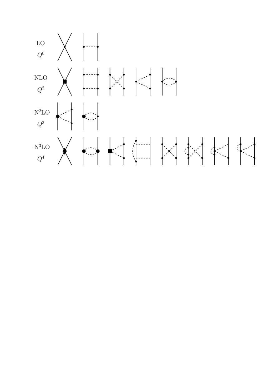
Figure 1: Relevant diagrams up-to-and-including N³LO. Solid and dashed lines denote antinucleons/nucleons and pions, respectively. The square and diamond symbolize contact vertices with two and four derivatives, respectively. The dot denotes a leading $\pi N$ vertex while the filled circle denotes a subleading $\pi N$ vertex. $Q$ denotes a small parameter (external momentum and/or pion mass).

2.1 Pion-exchange contributions

The one-pion exchange potential is given by

$$V_{1\pi}(q)=\biggl{(}\frac{g_{A}}{2F_{\pi}}\biggr{)}^{2}\,\left(1-\frac{p^{2}+p^{\prime 2}}{2m^{2}}\right)\mbox{\boldmath$\tau$}_{1}\cdot\mbox{\boldmath$\tau$}_{2}\,\frac{\mbox{\boldmath$\sigma$}_{1}\cdot{\bf q}\,\mbox{\boldmath$\sigma$}_{2}\cdot{\bf q}}{{\bf q}^{2}+M_{\pi}^{2}}\ ,$$ (1)

where ${\bf q}={\bf p}^{\prime}-{\bf p}$ is the transferred momentum defined in terms of the final (${\bf p}^{\prime}$) and initial (${\bf p}$) center-of-mass momenta of the baryons (nucleon or antinucleon). $M_{\pi}$ and $m$ denote the pion and antinucleon/nucleon mass, respectively. Following [42] relativistic $1/m^{2}$ corrections to the static one-pion exchange potential are taken into account already at NLO. As in the work [38] we take the larger value $g_{A}=1.29$ instead of $g_{A}=1.26$ in order to account for the Goldberger–Treiman discrepancy. This value, together with the used $F_{\pi}=92.4$ MeV, implies the pion-nucleon coupling constant $g_{NN\pi}=13.1$ which is consistent with the empirical value obtained from $\pi N$ and $NN$ data [46, 47] and also with modern determinations utilizing the GMO sum rule [48]. Contrary to [38], isospin-breaking in the hadronic interaction due to different pion masses is not taken into account. Here we use the isospin-averaged value $M_{\pi}=138.039$ MeV. The calculation of the $\bar{N}N$ phase shifts is done in the isospin basis and here we adopt the average nucleon value $m=938.918$ MeV. However, in the calculation of observables the mass difference between protons and neutrons is taken into account and the corresponding values from the PDG [49] are used.

Note that the contribution of one-pion exchange to the $\bar{N}N$ interaction is of opposite sign as that in $NN$ scattering. This sign difference arises from the G-parity transformation of the $NN\pi$ vertex to the $\bar{N}\bar{N}\pi$ vertex. The contributions from two-pion exchange to $NN$ and $\bar{N}N$ are identical. There would be again a sign differences for three-pion exchange. However, since the corresponding contributions are known to be weak we neglect them here as it was done in the $NN$ case [50].

The underlying effective pion-nucleon Lagrangian is given in Ref. [51]. For the LECs $c_{i}$ and $\bar{d}_{i}$ that appear in the subleading $\pi\pi NN$ vertices we take the same values as in Ref. [38]. Specifically, for $c_{1}$, $c_{3}$, and $c_{4}$ we adopt the central values from the $Q^{3}$–analysis of the $\pi N$ system [52], i.e. $c_{1}=-0.81$ GeV^-1, $c_{3}=-4.69$ GeV^-1, $c_{4}=3.40$ GeV^-1, while $c_{2}=3.28$ GeV^-1 is taken from the heavy-baryon calculation in Ref. [53]. However, in the future the more precise values of the $c_{i}$ determined from the Roy-Steiner analysis of pion-nucleon scattering [54] should be used for the $NN$ as well as the $\bar{N}N$ case. Note also that different values for the $c_{i}$ were used in the $\bar{N}N$ PWA [32]. Therefore, the two-pion exchange potential employed in our analysis differs from the one used for determining the $\bar{N}N$ phase shifts. However, based on the uncertainty estimate given in Ref. [32] we do not expect any noticeable effects from that on the quality of our results. In any case, it has to be said that our calculation includes also N³LO corrections to the two-pion exchange so that the corresponding potentials differ anyway.

In this context let us mention another difference to the analysis in Ref. [32]. It concerns the electromagnetic interaction where we consider only the (non-relativistic) Coulomb interaction in the $\bar{p}p$ system, but we neglect the magnetic-moment interaction.

2.2 Contact terms

The contact terms in partial-wave projected form are given by [38]

$$V(^{1}S_{0}) = \tilde{C}_{{}^{1}S_{0}}+{C}_{{}^{1}S_{0}}({p}^{2}+{p}^{\prime 2})+{D^{1}}_{{}^{1}S_{0}}{p}^{2}{p}^{\prime 2}+{D^{2}}_{{}^{1}S_{0}}({p}^{4}+{p}^{\prime 4})\,,$$ (2)

$$V(^{3}S_{1}) = \tilde{C}_{{}^{3}S_{1}}+{C}_{{}^{3}S_{1}}({p}^{2}+{p}^{\prime 2})+{D^{1}}_{{}^{3}S_{1}}{p}^{2}{p}^{\prime 2}+{D^{2}}_{{}^{3}S_{1}}({p}^{4}+{p}^{\prime 4})\,,$$ (3)

$$V(^{1}P_{1}) = {C}_{{}^{1}P_{1}}\,{p}\,{p}^{\prime}+{D}_{{}^{1}P_{1}}\,{p}\,{p}^{\prime}({p}^{2}+{p}^{\prime 2})\,,$$ (4)

$$V(^{3}P_{1}) = {C}_{{}^{3}P_{1}}\,{p}\,{p}^{\prime}+{D}_{{}^{3}P_{1}}\,{p}\,{p}^{\prime}({p}^{2}+{p}^{\prime 2})\,,$$ (5)

$$V(^{3}P_{0}) = {C}_{{}^{3}P_{0}}\,{p}\,{p}^{\prime}+{D}_{{}^{3}P_{0}}\,{p}\,{p}^{\prime}({p}^{2}+{p}^{\prime 2})\,,$$ (6)

$$V(^{3}P_{2}) = {C}_{{}^{3}P_{2}}\,{p}\,{p}^{\prime}+{D}_{{}^{3}P_{2}}\,{p}\,{p}^{\prime}({p}^{2}+{p}^{\prime 2})\,,$$ (7)

$$V(^{3}D_{1}-\,^{3}S_{1}) = {C}_{\epsilon_{1}}\,{p^{\prime}}^{2}+{D^{1}}_{\epsilon_{1}}{p}^{2}{p}^{\prime 2}+{D^{2}}_{\epsilon_{1}}{p}^{\prime 4}\,,$$ (8)

$$V(^{3}S_{1}-\,^{3}D_{1}) = {C}_{\epsilon_{1}}\,{p}^{2}+{D^{1}}_{\epsilon_{1}}{p}^{2}{p}^{\prime 2}+{D^{2}}_{\epsilon_{1}}{p}^{4}\,,$$ (9)

$$V(^{3}D_{1}) = {D}_{{}^{3}D_{1}}\,{p}^{2}{p}^{\prime 2}\,,$$ (10)

$$V(^{1}D_{2}) = {D}_{{}^{1}D_{2}}\,{p}^{2}{p}^{\prime 2}\,,$$ (11)

$$V(^{3}D_{2}) = {D}_{{}^{3}D_{2}}\,{p}^{2}{p}^{\prime 2}\,,$$ (12)

$$V(^{3}F_{2}-\,^{3}P_{2}) = {D}_{\epsilon_{2}}{p}{p}^{\prime 3}\,,$$ (13)

$$V(^{3}P_{2}-\,^{3}F_{2}) = {D}_{\epsilon_{2}}{p}^{3}{p}^{\prime}\,,$$ (14)

with $p=|{\bf p}\,|$ and ${p}^{\prime}=|{\bf p}\,^{\prime}|$. Here, the $\tilde{C}_{i}$ denote the LECs that arise at LO and that correspond to contact terms without derivates, the ${C}_{i}$ arise at NLO from contact terms with two derivates, and ${D}_{i}$ are those at N³LO from contact terms with four derivates. Note that the Pauli principle is absent in case of the $\bar{N}N$ interaction. Accordingly, each partial wave that is allowed by angular momentum conservation occurs in the isospin $I=0$ and in the $I=1$ channel. Therefore, there are now twice as many contact terms as in $NN$, that means $48$ up to N³LO.

The main difference between the $NN$ and $\bar{N}N$ interactions is the presence of annihilation processes in the latter. Since the total baryon number is zero, the $\bar{N}N$ system can annihilate and this proceeds via a decay into multi-pion channels, where typically annihilation into 4 to 6 pions is dominant in the low-energy region of $\bar{N}N$ scattering [1].

Since annihilation is a short-ranged process as argued in Ref. [42], in principle, it could be taken into account by simply using complex LECs in Eqs. (2)-(LABEL:VC). Indeed, this has been done in some EFT studies of $\bar{N}N$ scattering [55, 56]. However, with such an ansatz it is impossible to impose sensible unitarity conditions. Specifically, there is no guarantee that the resulting scattering amplitude fulfills the optical theorem, i.e. a requirement which ensures that for each partial wave the contribution to the total cross section is larger than its contribution to the integrated elastic cross section. Therefore, in Ref. [42] we treated annihilation in a different way so that unitarity is manifestly fulfilled already on a formal level. It consisted in considering the annihilation potential to be due to an effective two-body annihilation channel $X$ for each partial wave,

$$V_{ann}=V_{\bar{N}N\to X}G_{X}V_{X\to\bar{N}N},$$ (16)

with $V_{\bar{N}N\to X}$ the transition potential. Under the assumption that the threshold of $X$ is significantly below the one of $\bar{N}N$ the center-of-mass momentum in the annihilation channel is already fairly large and its variation in the low-energy region of $\bar{N}N$ scattering considered here can be neglected. Then the transition potential $V_{\bar{N}N\to X}$ can be represented by contact terms similar to the ones for $\bar{N}N\to\bar{N}N$, cf. Eqs. (2)-(LABEL:VC), and the Green’s function $G_{X}$ reduces to the unitarity cut, i.e. $G_{X}\propto-{\rm i}$. Note that Eq. (16) is exact under the assumption that there is no interaction in and no transition between the various annihilation channels.

The annihilation part of the $\bar{N}N$ potential is then of the form

$$V^{L=0}_{ann} = -i\,(\tilde{C}_{{}^{1}S_{0}}^{a}+C_{{}^{1}S_{0}}^{a}p^{2}+D_{{}^{1}S_{0}}^{a}p^{4})\,(\tilde{C}_{{}^{1}S_{0}}^{a}+C_{{}^{1}S_{0}}^{a}p^{\prime 2}+D_{{}^{1}S_{0}}^{a}p^{\prime 4}),$$ (17)

$$V^{L=1}_{ann} = -i\,(C_{\alpha}^{a}p+D_{\alpha}^{a}p^{3})\,(C_{\alpha}^{a}p^{\prime}+D_{\alpha}^{a}p^{\prime 3}),$$ (18)

$$V^{L=2}_{ann} = -i\,(D_{\beta}^{a})^{2}p^{2}p^{\prime 2},$$ (19)

$$V^{L=3}_{ann} = -i\,(D_{\gamma}^{a})^{2}p^{3}p^{\prime 3},$$ (20)

where $\alpha$ denotes the ${}^{3}P_{0}$, ${}^{1}P_{1}$, and ${}^{3}P_{1}$ partial waves, $\beta$ stands for ${}^{1}D_{2}$, ${}^{3}D_{2}$ and ${}^{3}D_{3}$, and $\gamma$ for ${}^{1}F_{3}$, ${}^{3}F_{3}$ and ${}^{3}F_{4}$. The superscript $a$ is used to distinguish the LECs from those in the elastic part of the $\bar{N}N$ potential. For the coupled ${}^{3}S_{1}-$${}^{3}D_{1}$ partial wave we use

$$V^{S\to S}_{ann} = -i\,(\tilde{C}_{{}^{3}S_{1}}^{a}+C_{{}^{3}S_{1}}^{a}p^{2}+D_{{}^{3}S_{1}}^{a}p^{4})\,(\tilde{C}_{{}^{3}S_{1}}^{a}+C_{{}^{3}S_{1}}^{a}p^{\prime 2}+D_{{}^{3}S_{1}}^{a}p^{\prime 4}),$$

$$V^{S\to D}_{ann} = -i\,(\tilde{C}_{{}^{3}S_{1}}^{a}+C_{{}^{3}S_{1}}^{a}p^{2}D_{{}^{3}S_{1}}^{a}p^{4})\,C_{\epsilon_{1}}^{a}p^{\prime 2},$$

$$V^{D\to S}_{ann} = -i\,C_{\epsilon_{1}}^{a}p^{2}\,(\tilde{C}_{{}^{3}S_{1}}^{a}+C_{{}^{3}S_{1}}^{a}p^{\prime 2}+D_{{}^{3}S_{1}}^{a}p^{\prime 4}),$$

$$V^{D\to D}_{ann} = -i\,[(C_{\epsilon_{1}}^{a})^{2}+(C_{{}^{3}D_{1}}^{a})^{2}]p^{2}p^{\prime 2}\ .$$ (21)

and for ${}^{3}P_{2}-$${}^{3}F_{2}$

$$V^{P\to P}_{ann} = -i\,(C_{{}^{3}P_{2}}^{a}p+D_{{}^{3}P_{2}}^{a}p^{3})\,(C_{{}^{3}P_{2}}^{a}p^{\prime}+D_{{}^{3}P_{2}}^{a}p^{\prime 3}),$$

$$V^{P\to F}_{ann} = -i\,(C_{{}^{3}P_{2}}^{a}p+D_{{}^{3}P_{2}}^{a}p^{3})\,D_{\epsilon_{2}}^{a}p^{\prime 3},$$

$$V^{F\to P}_{ann} = -i\,D_{\epsilon_{2}}^{a}p^{3}(C_{{}^{3}P_{2}}^{a}p^{\prime}+D_{{}^{3}P_{2}}^{a}p^{\prime 3}),$$

$$V^{F\to F}_{ann} = -i\,[(D_{\epsilon_{2}}^{a})^{2}+(D_{{}^{3}F_{2}}^{a})^{2}]p^{3}p^{\prime 3}\ .$$ (22)

In the expressions above the parameters $\tilde{C}^{a}$, $C^{a}$, and $D^{a}$ are real. There is no restriction on the signs of $\tilde{C}^{a}$, $C^{a}$, $D^{a}$ because the sign of $V_{ann}$ as required by unitarity is already explicitly fixed. Note, however, that terms of the form $p^{i}p^{\prime j}$ with higher powers $n=i+j$ than what follows from the standard Weinberg power counting arise in various partial waves from unitarity constraints and those have to be included in order to make sure that unitarity is fulfilled at any energy. Still we essentially recover the structure of the potential that follows from the standard power counting for $\bar{N}N\to\bar{N}N$ (cf. Eqs. (2)-(LABEL:VC)) with a similar (or even identical) number of counter terms (free parameters) for the annihilation part.

As one can see in Eq. (20) and also in Eq. (22) we allowed for contact terms in the annihilation potential for $F$ waves. This is motivated by two reasons. First, according to the PWA there is a nonzero contribution of $F$ waves to the annihilation cross section and we wanted to be able to take this into account. Second, as can be seen in Eq. (22), terms proportional to $p^{3}p^{\prime 3}$ appear anyway in the ${}^{3}F_{2}$ partial wave because of unitarity constraints. Moreover, transitions proportional to $p^{3}p^{\prime}$ (for ${}^{3}F_{2}\to$${}^{3}P_{2})$ are present in the real part at N³LO, see Eq. (LABEL:VC). This suggests that the analogous type of transitions should be taken into account in the description of annihilation via Eq. (16) from $F$ waves, i.e. $V^{F}_{\bar{N}N\to X}\equiv D^{a}_{F}p^{3}$. With regard to the real part of the $\bar{N}N$ (or $NN$) potential contact terms proportional to $p^{3}p^{\prime 3}$ would first appear at N⁵LO in the standard Weinberg counting and here we do not depart from the counting.

Note that, in principle, there is a contribution from the principal-value part of the integral in Eq. (16). However, it is real and, therefore, its structure is already accounted for by the standard LECs in Eqs. (2)–(LABEL:VC).

2.3 Scattering equation

As first step a partial-wave projection of the interaction potentials is performed, following the procedure described in detail in Ref. [37]. Then the reaction amplitudes are obtained from the solution of a relativistic Lippmann-Schwinger (LS) equation:

$$T_{L^{\prime\prime}L^{\prime}}(p^{\prime\prime},p^{\prime};E_{k})=V_{L^{\prime\prime}L^{\prime}}(p^{\prime\prime},p^{\prime})+\sum_{L}\int_{0}^{\infty}\frac{dpp^{2}}{(2\pi)^{3}}\,V_{L^{\prime\prime}L}(p^{\prime\prime},p)\frac{1}{2E_{k}-2E_{p}+i0^{+}}T_{LL^{\prime}}(p,p^{\prime};E_{k}).$$

(23)

Here, $E_{k}=\sqrt{m^{2}+k^{2}}$, where $k$ is the on-shell momentum. We adopt a relativistic scattering equation so that our amplitudes fulfill the relativistic unitarity condition at any order, as done also in the $NN$ sector [37, 40]. On the other hand, relativistic corrections to the potential are calculated order by order. They appear first at next-to-next-to-next-to-leading order (N³LO) in the Weinberg scheme, see A.

Analogous to the $NN$ case we have either uncoupled spin-singlet and triplet waves (where $L^{\prime\prime}=L^{\prime}=L=J$) or coupled partial waves (where $L^{\prime\prime},L^{\prime},L=J-1,J+1$). The LECs of the $\bar{N}N$ potential are determined by a fit to the phase shifts and inelasticity parameters of Ref. [32]. Those quantities were obtained under the assumption of isospin symmetry and, accordingly, we solve the LS equation in the isospin basis where the $I=0$ and $I=1$ channels are decoupled. For the calculation of observables, specifically for the direct comparison of our results with data, we solve the LS equation in particle basis. In this case there is a coupling between the $\bar{p}p$ and $\bar{n}n$ channels. The corresponding potentials are given by linear combinations of the ones in the isospin basis, i.e. $V^{\bar{p}p}=V^{\bar{n}n}=(V^{I=0}+V^{I=1})/2$ and $V^{\bar{p}p\leftrightarrow\bar{n}n}=(V^{I=0}-V^{I=1})/2$. Note that the solution of the LS equation in particle basis no longer fulfills isospin symmetry. Due to the mass difference between $p$ ($\bar{p}$) and $n$ ($\bar{n}$) the physical thresholds of the $\bar{p}p$ and $\bar{n}n$ channels are separated by about 2.5 MeV. In addition the Coulomb interaction is present in the $\bar{p}p$ channel. Both effects are included in our calculation where the latter is implemented via the Vincent-Phatak method [57]. Other electromagnetic effects like those of the magnetic-moment interaction, considered in Ref. [32] are, however, not taken into account in our calculation.

The relation between the $S$– and on–the–energy shell $T$–matrix is given by

$$S_{LL^{\prime}}(k)=\delta_{LL^{\prime}}-\frac{i}{8\pi^{2}}\,k\,E_{k}\,T_{LL^{\prime}}(k)~{}.$$ (24)

The phase shifts in the uncoupled cases can be obtained from the $S$–matrix via

$$S_{LL}\equiv S_{L}=e^{2i\delta_{L}}\,.$$ (25)

For the $S$–matrix in the coupled channels ($J>0$) we use the so–called Stapp parametrization [58]

$$\left(\begin{array}[]{cc}S_{J-1\,J-1}&S_{J-1\,J+1}\\ S_{J+1\,J-1}&S_{J+1\,J+1}\end{array}\right)=\left(\begin{array}[]{cc}\cos{2\epsilon_{J}}\,e^{2i\delta_{J-1}}&-i\sin{2\epsilon_{J}}\,e^{i(\delta_{J-1}+\delta_{J+1})}\\ -i\sin{2\epsilon_{J}}\,e^{i(\delta_{J-1}+\delta_{J+1})}&\cos{2\epsilon_{J}}\,e^{2i\delta_{J+1}}\end{array}\right)~{}.$$ (30)

In case of elastic scattering the phase parameters in Eqs. (25) and (30) are real quantities while in the presence of inelasticities they become complex. Because of that, in the past several generalizations of these formulae have been proposed that still allow one to write the $S$-matrix in terms of real parameters [59, 32]. We follow here Ref. [60] and calculate/present simply the real and imaginary parts of the phase shifts and the mixing parameters obtained via the above parameterization. Note that with this choice the real part of the phase shifts is identical to the phase shifts one obtains from another popular parameterization where the imaginary part is written in terms of an inelasticity parameter $\eta$, e.g. for uncoupled partial waves

$$S_{L}=\eta e^{2i\delta_{L}}\;.$$ (31)

Indeed, for this case ${\rm Im}\,\delta_{L}=-(\log\eta)/2$ which implies that ${\rm Im}\,\delta_{L}\geq 0$ since $\eta\leq 1$ because of unitarity. Note that for simplicity reasons, in the discussion of the results below we will refer to the real part of the phase shift as phase shift and to the imaginary part as inelasticity parameter. Since our calculation implements unitarity, the optical theorem

$${\rm Im}\,a_{LL}(k)\geq k\,\sum_{L^{\prime}}|a_{LL^{\prime}}(k)|^{2}\ ,$$ (32)

is fulfilled for each partial wave, where $a_{LL^{\prime}}(k)=(S_{LL^{\prime}}-\delta_{LL^{\prime}})/(2ik)=-1/(4\pi)^{2}\cdot E_{k}\,T_{LL^{\prime}}(k)$.

For the fitting procedure and for the comparison of our results with those of Ref. [32] we reconstructed the $S$-matrix based on the phase shifts listed in Tables VIII-X of that paper via the formulae presented in Sect. VII of that paper and then converted them to our convention specified in Eqs. (25) and (30).

3 Fitting procedure and estimation of the theoretical uncertainty

An important objective of the work of Ref. [38] consisted in a careful analysis of the cutoff dependence and in providing an estimation of the theoretical uncertainty. The reasoning for making specific assumptions, and adopting and following specific procedures in order to achieve that aim has been explained and thoroughly discussed in that paper and we do not repeat this here in detail. However, we want to emphasize that whatever has been said there for $NN$ scattering is equally valid for the $\bar{N}N$ system. It is a consequence of the fact that the general structure of the long-range part of the two interactions is identical – though the actual potential strengths in the individual partial waves certainly differ. Accordingly, the non-local exponential regulator employed in [37, 43] but also in our N²LO study of $\bar{N}N$ scattering [42] for the one- and two-pion exchange contributions will be replaced here by the new regularization scheme described in Sect. 3 of [38]. This scheme relies on a regulator that is defined in coordinate space and, therefore, is local by construction. As demonstrated in that reference, the use of a local regulator is superior at higher energies and, moreover, produces a much smaller amount of artefacts over the whole considered energy range. The contact interactions are non-local anyway, cf. Eqs. (2)-(LABEL:VC). In this case we use again the standard nonlocal regulator of Gaussian type. The explict form of the cutoff functions employed in the present study is given by

$$f(r)=\left[1-{\rm exp}\left(-\frac{r^{2}}{R^{2}}\right)\right]^{n},\quad f(p^{\prime},p)={\rm exp}\left(-\frac{p^{\prime m}+p^{m}}{\Lambda^{m}}\right)\ .$$ (33)

For the cutoffs we consider the same range as in Ref. [38], i.e from $R=0.8$ fm to $R=1.2$ fm. The cutoff in momentum-space applied to the contact interactions is fixed by the relation $\Lambda=2R^{-1}$ so that the corresponding range is then $\Lambda\simeq 500,...,300$ MeV. Following [38], the exponent in the coordinate-space cutoff function is chosen to be $n=6$, the one for the contact terms in momentum space to be $m=2$.

3.1 Fitting procedure

In the fitting procedure we follow very closely the strategy of Ref. [38] in their study of the $NN$ interaction. The LECs are fixed from a fit to the $\bar{N}N$ phase shifts and mixing parameters of Ref. [32] where we take into account their results for $p_{lab}\leq 300$ MeV/c ($T_{lab}\leq 50$ MeV) at LO, $p_{lab}\leq 500$ MeV/c ($T_{lab}\leq 125$ MeV) at NLO and N²LO, and $p_{lab}\leq 600$ MeV/c ($T_{lab}\leq 175$ MeV) at N³LO. Exceptions are made in cases where the phase shifts (or inelasticity parameters) exhibit a resonance-like behavior at the upper end of the considered momentum interval. Then we extend or reduce the energy range slightly in order to stabilize the results and avoid artefacts.

No uncertainties are given for the $\bar{N}N$ phase shifts and inelasticity parameters of the PWA. Because of that we adopt a constant and uniform value $\Delta$ for them for the evaluation of the function to which the minimization procedure is applied. Thus, the uncertainty is reduced simply to an overall normalization factor. On top of that, additional weight factors are introduced in the fitting process in a few cases where it turned out to be difficult to obtain stable results. The $\tilde{\chi}^{2}$ values summarized in Table 1 for orientation are, however, all calculated with a universal $\Delta$ which was set to $\Delta^{2}=0.1$. The tilde is used as a reminder that these are not genuine chi-square values. The actual $\tilde{\chi}^{2}$ function in the fitting procedure for each partial wave is $|S_{LL^{\prime}}-S^{PWA}_{LL^{\prime}}|^{2}/\Delta^{2}$ where the $S$-matrix elements $S^{PWA}_{LL^{\prime}}$ are reconstructed from the phase shifts and inelasticity parameters given in Tables VIII-X of Ref. [32].

Table 1 reveals that the lowest values for the $\tilde{\chi}^{2}$ are achieved for hard cutoffs, namely $R=0.8-0.9$ fm. This differs slightly from the $NN$ case where somewhat softer values $R=0.9-1.0$ fm seem to be preferred. In both cases a strong increase in the $\tilde{\chi}^{2}$ is observed for the softest cutoff radius considered, i.e. for $R=1.2$ fm. For the illustration of our results we will use, in general, the interaction with the cutoff $R=0.9$ fm. That value was found to be the optimal cutoff choice in the $NN$ study [38]. Nominally, in terms of the $\tilde{\chi}^{2}$ value, $R=0.8$ fm would be the optimal cutoff choice for $\bar{N}N$. But the differences in the quality of the two fits are so small, see Table 1, that we do not attribute any significance to them given that no proper chi-square can be calculated. The numerical values of the LECs are compiled in Tables in B.

Table 1: Resulting effective $\tilde{\chi}^{2}$ (see text) for different cutoffs and different energy regions.

$\tilde{\chi}^{2}$	R=0.8 fm	R=0.9 fm	R=1.0 fm	R=1.1 fm	R=1.2 fm
$T_{lab}\leq 25$ MeV	0.003	0.004	0.004	0.019	0.036
$T_{lab}\leq 100$ MeV	0.023	0.025	0.036	0.090	0.176
$T_{lab}\leq 200$ MeV	0.106	0.115	0.177	0.312	0.626
$T_{lab}\leq 300$ MeV	2.012	2.171	3.383	5.531	9.479

3.2 Estimation of the theoretical uncertainty

The motivation and the strategy, and also the shortcomings, of the procedure for estimating the theoretical uncertainty suggested in Ref. [38] are discussed in detail in Sect. 7 of that reference. The guiding principle behind that suggestion is that one uses the expected size of higher-order corrections for the estimation of the theoretical uncertainty. This is commonly done, e.g. in the Goldstone boson and single-baryon sectors of chiral perturbation theory. This approach is anticipated to provide a natural and more reliable estimate than relying on cutoff variations, say, as done in the past, and, moreover, it has the advantage that it can be applied for any fixed value of the cutoff $R$.

The concrete expression used in this approach to calculate an uncertainty $\Delta X^{\rm N^{3}LO}(k)$ to the N³LO prediction $X^{\rm N^{3}LO}(k)$ of a given observable $X(k)$ is [38]

$$\Delta X^{\rm N^{3}LO}(k) = \max\bigg{(}Q^{5}\times\Big{|}X^{\rm LO}(k)\Big{|},\;\;\;Q^{3}\times\Big{|}X^{\rm LO}(k)-X^{\rm NLO}(k)\Big{|},\;\;\;Q^{2}\times\Big{|}X^{\rm NLO}(k)-X^{\rm N^{2}LO}(k)\Big{|},$$ (34)

$${}\;\;\;\;\;\;\;\;\;\;Q\times\Big{|}X^{\rm N^{2}LO}(k)-X^{\rm N^{3}LO}(k)\Big{|}\bigg{)}\,,$$

where the expansion parameter $Q$ is defined by

$$Q=\max\left(\frac{k}{\Lambda_{b}},\;\frac{M_{\pi}}{\Lambda_{b}}\right)\,,$$ (35)

with $k$ the cms momentum corresponding to the considered laboratory momentum and $\Lambda_{b}$ the breakdown scale. For the latter we take over the values established in Ref. [38] which are $\Lambda_{b}=600\,$MeV for the cutoffs $R=0.8$, $0.9$ and $1.0\,$fm, $\Lambda_{b}=500\,$MeV for $R=1.1\,$fm and $\Lambda_{b}=400\,$MeV for $R=1.2$. Analogous definitions are used for calculating the uncertainty up to N²LO, etc. Note that the quantity $X(k)$ represents not only a “true” observable such as a differential cross section or an analyzing power, but also for a phase shift or an inelasticity parameter.

As already emphasized in [38], such a simple estimation of the theoretical uncertainty does not provide a statistical interpretation. Note, however, that this procedure can be interpreted in a Bayesian sense [45]. Let us also mention that – like in [38] – we impose an additional constraint for the theoretical uncertainties at NLO and N²LO by requiring them to have at least the size of the actual higher-order contributions.

4 Results

4.1 Phase shifts

Let us first consider the influence of cutoff variations on our results. In Figs. 2-4 phase shifts and inelasticity parameters for partial waves up to a total angular momentum of $J=4$ are presented. We use here the spectral notation ${}^{(2S+1)}L_{J}$ and indicate the isospin $I$ separately. Subscripts $R$ and $I$ are used for $\delta$ in order to distinguish between the real and imaginary part of the phases and mixing angles. The cutoffs considered are $R=0.8$, $0.9$, $1.0$, $1.1$, and $1.2$ fm and the results are based on the chiral potential up to N³LO.

One can see that for most partial waves the cutoff dependence is fairly weak for $T_{lab}$ up to $300$ MeV ($p_{lab}$ up to $800$ MeV/c). Indeed, the small residual cutoff dependence that we observe here is comparable to the likewise small variation reported in Ref. [38] for the $NN$ interaction. Only in a few cases there is a more pronounced cutoff dependence of the results for energies above $150$-$200$ MeV. This has to do with the fact that the PWA [32] suggests a resonance-like behavior of some phases in this region. This concerns most prominently the ${}^{1}S_{0}$ partial wave with isospin $I=1$ and the ${}^{3}P_{0}$ partial wave with $I=1$. In addition, also a few other partial waves show a conspicuous behavior at higher energies in the sense that the energy dependence changes noticeably. Typical examples are the inelasticity parameters for the $I=0$ ${}^{3}P_{0}$ and ${}^{3}P_{2}$ partial wave, where the corresponding $\delta_{\rm I}$’s increase rapidly from the threshold, but then level out at higher energies. Describing this behavior with the two LECs at N³LO, that have to absorb the cutoff dependence at the same time, is obviously only possible for a reduced energy region.

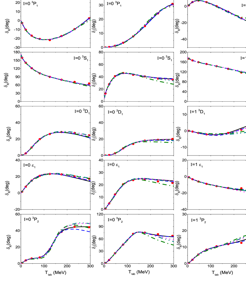
Figure 2: Real and imaginary parts of various $\bar{N}N$ phase shifts at N³LO for cutoffs $R=0.8-1.2$ fm. The filled circles represent the solution of the $\bar{p}p$ PWA [32].

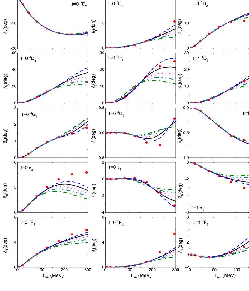
Figure 3: Real and imaginary parts of various $\bar{N}N$ phase shifts at N³LO for cutoffs $R=0.8-1.2$ fm. The filled circles represent the solution of the $\bar{p}p$ PWA [32].

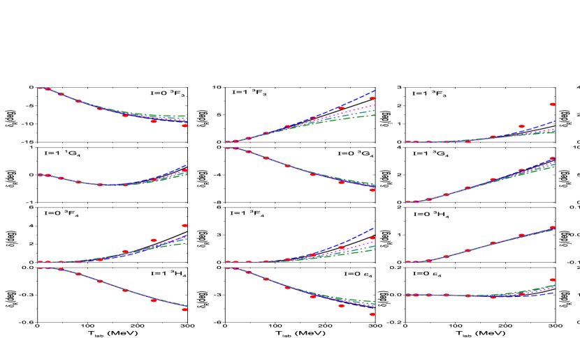
Figure 4: Real and imaginary parts of various $\bar{N}N$ phase shifts at N³LO for cutoffs $R=0.8-1.2$ fm. The filled circles represent the solution of the $\bar{p}p$ PWA [32].

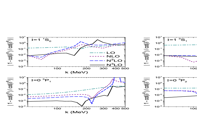
Figure 5: Error plot for the real part of the phase shifts for the isospin $I=1$ partial waves ${}^{1}S_{0}$, ${}^{3}S_{1}$ and and for the $I=0$ ${}^{3}P_{1}$, ${}^{3}P_{2}$ partial waves. Here $R_{1}=0.9$ fm and $R_{2}=1.0$ fm. The black/solid line is at N³LO, the blue/dashed line at N²LO, the magenta/dotted line at NLO, and the green/dash-double-dotted line corresponds to the LO result.

For a more quantitative assessment of the residual cutoff dependence of the phase shifts and inelasticity parameters in a given channel we follow the procedure described in Refs. [38, 61]. In these works the quantity $|1-\cot\delta^{(R_{1})}(k)/\cot\delta^{(R_{2})}(k)|$ is considered as function of the cms momentum $k$, where $R_{1}$ and $R_{2}$ are two different values of the cutoff. Since in the $\bar{N}N$ case the phase shifts are complex, we examine that quantity for the real part of $\delta$ ($\delta_{R}$) and for the imaginary part ($\delta_{I}$) separately, i.e. we evaluate $|1-\cot\delta^{(R_{1})}_{R}(k)/\cot\delta^{(R_{2})}_{R}(k)|$ and $|1-\cot\delta^{(R_{1})}_{I}(k)/\cot\delta^{(R_{2})}_{I}(k)|$. Corresponding results for selected partial waves can be found in Fig. 5 for the particular choice of $R_{1}=0.9\,$fm and $R_{2}=1.0\,$fm.

According to Ref. [38] the residual cutoff dependence can be viewed as an estimation of effects of higher-order contact interactions beyond the truncation level of the potential. Given that there are no new contact terms when going from the chiral orders NLO and N²LO, cf. Sect. 2.2, one expects that the residual cutoff dependence reduces only when going from LO to NLO and then again from N²LO to N³LO. Indeed, the results presented in Fig. 5 demonstrate that the cutoff dependence at NLO and N²LO is comparable. Furthermore, there is a noticeable reduction of the cutoff dependence over a larger momentum range when going from LO to NLO/N²LO and (in case of the $P$-waves) from NLO/N²LO to N³LO. Thus, despite certain limitations, overall the behavior we observe here for the $\bar{N}N$ phase shifts is similar to that in the $NN$ case [38]. This applies roughly also to the breakdown scale $\Lambda_{b}$ at N³LO, that is to the momentum at which the N³LO curves cross the ones of lower orders. In the $NN$ section it was argued that $\Lambda_{b}$ is about $\sim 500\,$MeV for $S$-waves and even higher for $P$-waves [38]. Based on the results in Fig. 5 we would draw a similar conclusion for the $\bar{N}N$ interaction.

In any case, we want to emphasize that caution has to be exercised in the interpretation of the error plots. Specifically, one should not forget that they provide only a qualitative guideline [38]. In this context we want to comment also on the dips or other sharp structures in the error plots. Those appear at values of $k$ where the function $1-\cot\delta^{(R_{1})}(k)/\cot\delta^{(R_{2})}(k)$ changes its sign or where one of the phase shifts crosses $0$ or $90$ degrees. As already pointed out in Ref. [38] those have no significance and should be ignored. Indeed, a notable number of $\bar{N}N$ phase shifts exhibit a strong energy dependence and, thus, cross $0$ or $90$ degrees, cf. Figs. 2-4. Because of that the kind of artefacts mentioned above occur more often in $\bar{N}N$, especially in $S$-waves. Accordingly, those distort the error plots more than what happened for the $NN$ phase shifts and make their interpretation more delicate.

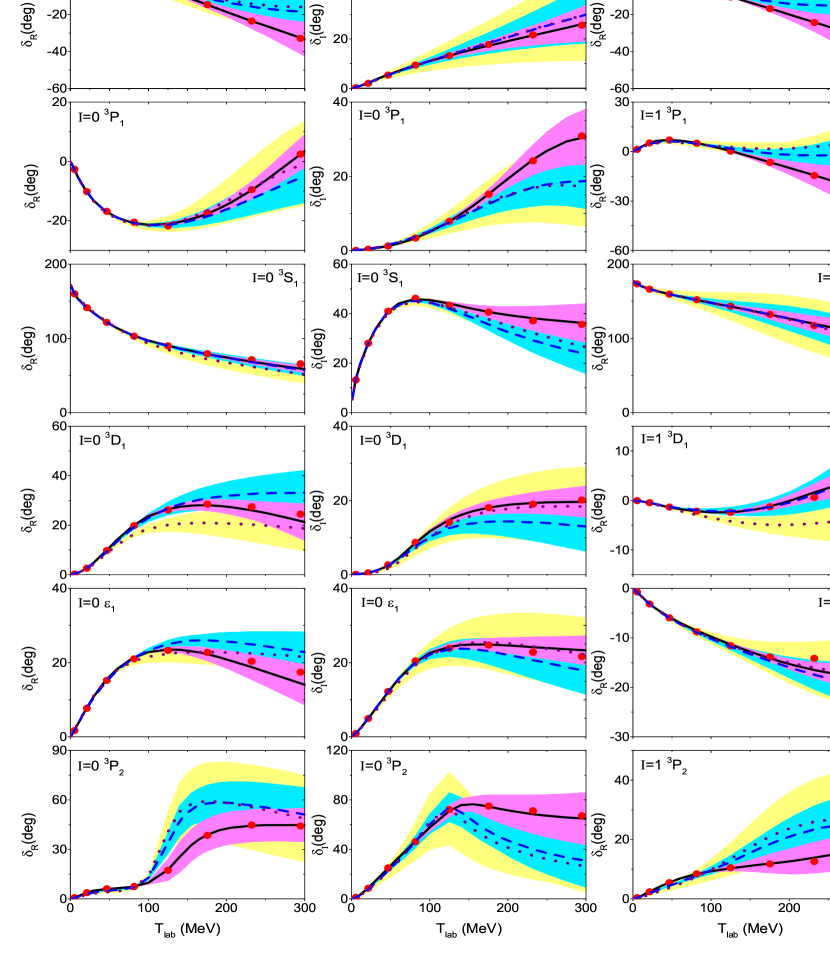
Figure 6: Real and imaginary parts of various $\bar{N}N$ phase shifts for the potential with cutoff $R=0.9$ fm. Results at N³LO (black/solid line), N²LO (blue/dashed line), and NLO (magenta/dotted line) are shown. Uncertainty bands at N³LO (dark/magenta), N²LO (medium/cyan), and NLO (light/yellow) are included. The filled circles represent the solution of the $\bar{p}p$ PWA [32].

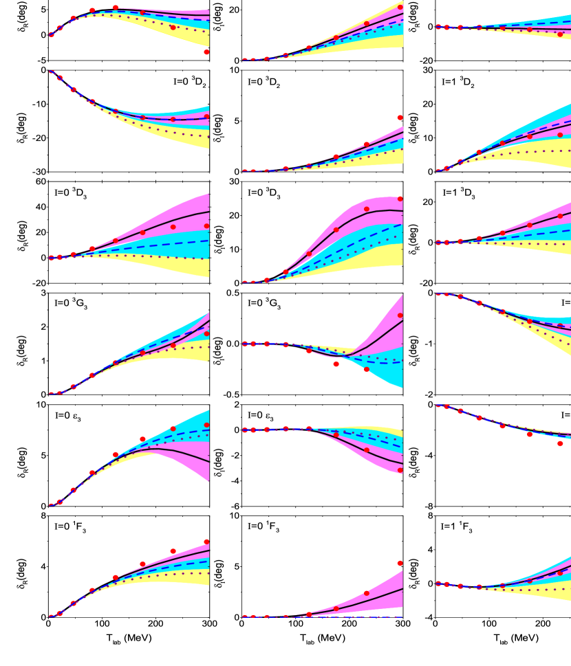
Figure 7: Real and imaginary parts of various $\bar{N}N$ phase shifts for the potential with cutoff $R=0.9$ fm. For notations, see Fig. 6.

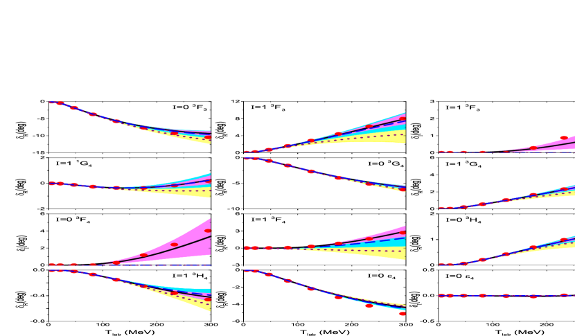
Figure 8: Real and imaginary parts of various $\bar{N}N$ phase shifts for the potential with cutoff $R=0.9$ fm. For notations, see Fig. 6.

The phase shifts and mixing angles for the cutoff $R=0.9\,$fm are again presented in Fig. 6-8. However, now results at NLO (dotted curves), N²LO (dashed curves) and N³LO (solid curves) are shown and, in addition, the uncertainty estimated via Eq. (34) is indicated by bands. The results of the $\bar{N}N$ PWA [32] are displayed by circles. There is a clear convergence visible from the curves in those figures for most partial waves. Moreover, in case of $S$- and $P$-waves the N³LO results are in excellent agreement with the PWA in the whole considered energy range, i.e. up to $T_{lab}=300$ MeV. This is particularly remarkable for channels where there is a resonance-like behavior like in the isospin $I=1$ ${}^{1}S_{0}$ and ${}^{3}P_{0}$ states, see Fig. 6. Note that even for higher partial waves the phase shifts and inelasticities are well described at least up to energies of $200$ to $250$ MeV at the highest order considered, as can be seen in Figs. 7 and 8.

Overall, the convergence pattern is qualitatively similar to the one for the corresponding $NN$ partial waves reported in Ref. [38]. Exceptions occur, of course, in those $\bar{N}N$ waves where the PWA predicts a resonance-like behavior. Furthermore, also with regard to the uncertainty estimate, represented by bands in Figs. 6-8, in general, the behavior resembles the one observed in the application of chiral EFT to $NN$ scattering. Specifically, it is reassuring to see that in most cases also for $\bar{N}N$ the uncertainty as defined in Eq. (34) fulfills the conditions and expectations discussed in Sect. 7 of Ref. [38]. Thus, we conclude that the approach for error estimation suggested in Ref. [38] is well applicable for the $\bar{N}N$ case, too.

Some more detailed observations: It is interesting to see that in the ${}^{1}S_{0}$, ${}^{3}P_{0}$ and ${}^{3}S_{1}$ partial waves with $I=0$ the uncertainty is very small, even at $T_{lab}=300$ MeV, just like what was found for the corresponding $NN$ states. On the other hand, and not unexpected, there is a much larger uncertainty in the $I=1$ state, in particular in the ${}^{1}S_{0}$ and ${}^{3}P_{0}$ waves. Again this has to do with the resonance-like behavior. As noted above, these structures can be reproduced quantitatively only at the highest order and the poorer convergence in this case is then reflected in a larger uncertainty - as it should be according to its definition, see Eq. (34). Such a resonance-like behavior and/or an “unusually” strong energy dependence at higher energies of phase shifts is also the main reason why for some cases the uncertainty estimate fails to produce the desired results, i.e. where the bands do not show a monotonic behavior, where they do not overlap for different orders, or where the PWA results lie outside of the uncertainty bands. Examples for that are the inelasticity for ${}^{1}S_{0}$ with $I=1$, the inelasticity for ${}^{3}P_{0}$ with $I=1$, or the ${}^{3}P_{2}$ and ${}^{3}F_{2}$ phase shifts and the mixing angle $\epsilon_{2}$ with $I=0$. Note that in many cases there is a larger uncertainy for the inelasticity than for the phase shift itself. Again this is not unexpected. For $P$- and higher partial waves nonzero results for the inelasticity are only obtained from NLO onwards in the power counting we follow so that the convergence is slower. Finally, let us mention that in some $F$-, $G$-, and $H$-waves the inelasticity is zero or almost zero [32]. We omitted the corresponding graphs from Fig. 8.

4.2 Observables

In our first study of $\bar{N}N$ scattering within chiral EFT [42] we focused on the phase shifts and inelasticities. Observables were not considered. One reason for this was that, at that time, our computrt code was only suitable for calculations in the isospin basis. A sensible calculation of observables, specifically at low energies where chiral EFT should work best, has to be done in the particle basis because the Coulomb interaction in the $\bar{p}p$ system has to be taken into account and also the mass difference between proton and neutron. The latter leads to different physical thresholds for the $\bar{p}p$ and $\bar{n}n$ channels which has a strong impact on the reaction amplitude close to those thresholds.

Another reason is related directly to the dynamics of $\bar{N}N$ scattering, specifically to the presence of annihilation processes. Annihilation occurs predominantly at short distances and yields a reduction of the magnitude of the $S$-wave amplitudes. Because of that, higher partial waves start to become important at much lower energies as compared to what one knows from the $NN$ interaction [3]. Thus, already at rather moderate energies a realistic description of higher partial waves, in particular of the $P$- as well as $D$-waves, is required for a meaningful confrontation of the computed amplitudes with scattering data.

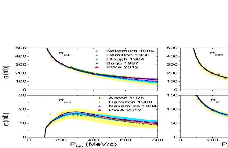
Figure 9: Total ($\sigma_{tot}$) and integrated elastic ($\sigma_{el}$), charge-exchange ($\sigma_{cex}$), and annihilation ($\sigma_{ann}$) cross sections for $\bar{p}p$ scattering. Results at N³LO (black/solid line), N²LO (blue/dashed line), and NLO (magenta/dotted line) are shown. Uncertainty bands at N³LO (dark/magenta), N²LO (medium/cyan), and NLO (light/yellow) are included. The filled circles represent the solution of the $\bar{p}p$ PWA [32]. Data are taken from Refs. [62, 63, 64, 65] ($\sigma_{tot}$), [66, 67, 68] ($\sigma_{ann}$), [69, 70, 71] ($\sigma_{cex}$), and [72, 73, 74] ($\sigma_{el}$).

In the present paper we extended our chiral EFT $\bar{N}N$ potential to N³LO. At that order the first LECs in the $D$-waves appear, cf. Eq. (LABEL:VC), and can be used to improve substantially the reproduction of the corresponding partial-wave amplitudes of the $\bar{N}N$ PWA, cf. Figs. 6 and 7. Thus, it is now timely to perform also a calculation of observables and compare those directly with measurements. Integrated cross sections are shown in Fig. 9. Results are provided for the total reaction cross section, for the total annihilation cross section, and for the integrated elastic ($\bar{p}p\to\bar{p}p$) and charge-exchange ($\bar{p}p\to\bar{n}n$) cross sections. Similar to the presentation of the phase shifts before, we include curves for the NLO (dotted lines), N²LO (dashed lines), and N³LO (solid lines) results and indicate the corresponding uncertainty estimate by bands for the cutoff $R=0.9\,$fm. The LO calculation is not shown because it provides only a very limited and not realistic description of observables. Instead we include a variety of experimental results.

Before discussing the results in detail let us make a general comment on the data. We display experimental information primarily for illustrating the overall quality of our results. Thus, we choose specific measurements at specific energies which fit best to that purpose, and we use the values as published in the original papers. This differs from the procedure in the PWA [32] where data selection is done and has to be done. After all, one cannot do a dedicated PWA without having a self-consistent data set. Thus, normalization factors are introduced for the data sets in the course of the PWA and some data have been even rejected. For details on the criteria employed in the PWA and also for individual information on which data sets have been renormalized or rejected we refer the reader to Ref. [32]. In view of this it is important to realize that there can be cases where our EFT interaction reproduces the PWA perfectly but differs slightly from the real data (when a renormalization was employed) or even drastically (when those data were rejected). Of course, in the latter case we will emphasize that in the discussion.

Our results for the integrated cross sections at N³LO, indicated by solid lines in Fig. 9, agree rather well with the ones of the PWA (filled circles), even up to $p_{lab}=800$ MeV/c. Indeed, also the charge-exchange cross section is nicely reproduced, though it is much smaller than the other ones. The amplitude for this process is given by the difference of the $I=0$ and $I=1$ amplitudes and its description requires a delicate balance between the interactions in the corresponding isospin channels. Obviously, this has been achieved with our chiral EFT interaction. Note that there are inconsistencies in the charge-exchange measurements at low energies and some of the data in question have not been taken into account in the PWA, cf. Table III in [32]. Considering the bands presenting the estimate of the uncertainty, one can see that there is a clear convergence of our results for all cross sections when going to higher orders. Finally, as a further demonstration of the quality of our N³LO results we summarize partial-wave cross sections for $\bar{p}p$ elastic and charge-exchange scatting in Table 2. Obviously, there is nice agreement with the values from the PWA for basically all $S$- and $P$-waves.

Table 2: Partial-wave cross sections predicted by the chiral potential at N³LO with $R=0.9$ fm in comparison to results from the $\bar{N}N$ partial wave analysis [32].

		$\bar{p}p\to\bar{p}p$				$\bar{p}p\to\bar{n}n$
	$p_{lab}$ (MeV/c)	200	400	600	800	200	400	600	800
${}^{1}S_{0}$	N3LO	15.9	8.0	4.1	2.0	0.7	0.1
	PWA	15.7	7.9	4.1	2.1	0.7	0.1
${}^{3}S_{1}$	N3LO	66.6	25.9	13.1	8.0	2.9	0.9	0.5	0.3
	PWA	66.1	26.0	13.2	8.8	3.0	1.0	0.5	0.2
${}^{3}P_{0}$	N3LO	4.9	5.4	5.1	3.6	1.5	0.8	0.1
	PWA	4.9	5.4	5.0	3.5	1.5	0.8	0.1
${}^{1}P_{1}$	N3LO	1.0	2.5	4.4	5.6	0.8	0.1
	PWA	0.9	2.5	4.5	5.6	0.8	0.1
${}^{3}P_{1}$	N3LO	1.8	5.0	4.1	3.6	5.1	3.0	0.2	0.1
	PWA	1.8	4.9	4.0	3.5	4.9	2.9	0.2	0.1
${}^{3}P_{2}$	N3LO	7.0	17.1	14.1	9.9	1.0	1.5	0.4	0.1
	PWA	7.0	17.0	13.9	9.6	0.9	1.4	0.4	0.1

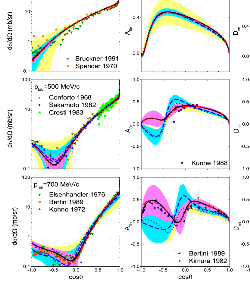
Figure 10: Differential cross sections, analyzing powers and spin correlation parameters $D_{nn}$ for $\bar{p}p$ elastic scattering. For notations, see Fig. 9. The red/dash-double dotted line represents the result of the PWA [32]. Data are taken from Refs. [75, 67, 76, 73, 77, 78, 79, 80] (differential cross sections), [81, 82, 83] (analyzing powers), and [84] ($D_{nn}$).

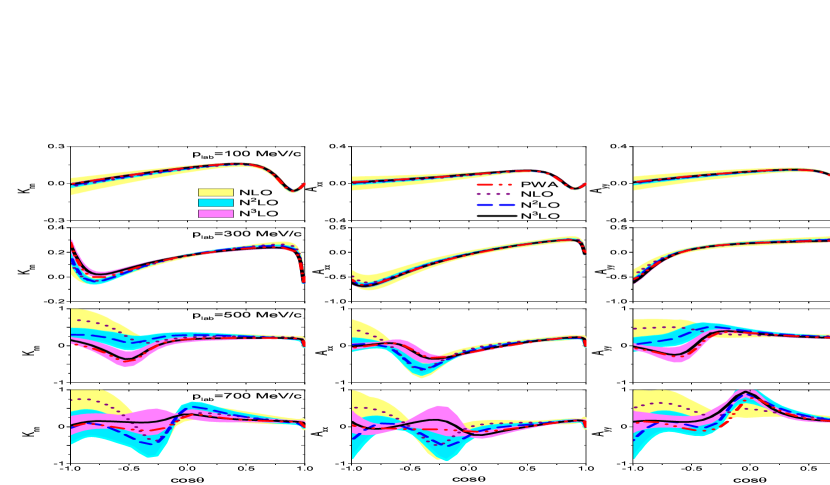
Figure 11: Spin correlation parameters $K_{nn}$, $A_{xx}$, $A_{yy}$, and $A_{zz}$ for $\bar{p}p$ elastic scattering. For notations, see Fig. 10.

Differential cross sections, analyzing powers and the spin-correlation parameters $D_{nn}$ for $\bar{p}p$ elastic scattering are shown in Fig. 10. Results for further spin-dependent observables can be found in Fig. 11. We selected results at the momenta $100$, $300$, $500$, and $700$ MeV/c ($T_{lab}=$ $5.32$, $46.8$, $125$, and $232$ MeV) for the presentation because that allows us to compare with some existing measurements (for $d\sigma/d\Omega$, $A_{on}$) and it allows us also to document how the quality of the description of $\bar{N}N$ scattering observables by our EFT interaction develops with increasing energy. The results of the $\bar{N}N$ PWA [32] are indicated by dash-dotted lines. Since only $\bar{N}N$ partial waves up to $J=4$ are tabulated in Ref. [32] we supplemented those by amplitudes from our N³LO interaction for higher angular momenta in the evaluation of differential observables. As already emphasized above, those amplitudes differ to some extent from the ones used in the PWA itself. But we do not expect that those differences have a strong influence on the actual results. Note that contributions from $J\geq 5$ become relevant for momenta above $400$ MeV/c, but primarily at backward angles.

In principle, at the lowest energy considered, $T_{lab}=5.32$ MeV, we expect excellent agreement of our calculation with the PWA. However, one has to keep in mind that we fitted to the phase shifts and inelasticies in the isospin basis. The observables are calculated from partial-wave amplitudes in the particle basis. The latter are obtained by solving the corresponding LS equation where then the hadronic interaction is modified due to the presence of the Coulomb interaction, and there are additional kinematical effects from the shift of the $\bar{n}n$ threshold to its physical value. Therefore, it is not trivial that we agree so well with the PWA results, that are generated from the $S$-matrix elements in the particle basis as listed in Ref. [32]. Actually, in case of the differential cross section one cannot distinguish the corresponding (solid, dash-dotted) lines in the figure. The estimated uncertainty is also rather small at least for the differential cross section. Spin-dependent observables involve contributions from higher partial waves from the very beginning and because of that the uncertainties are larger, especially for the lower-order results. There is no experimental information on differential observables at such low energies.

Naturally, when we go to higher energies the uncertainty increases. In this context we want to point out that the differential cross section exhibits a rather strong angular dependence already at $p_{lab}=300$ MeV/c. Its value drops by more than one order of magnitude with increasing angles, cf. Fig. 10. This means that at backward angles there must be a delicate cancellation between many partial-wave amplitudes and, accordingly, a strong sensitivity to the accuracy achieved in each individual partial wave. Note also that a logarithmic scale is used that optically magnifies the size of the uncertainty bands for small values. The behavior of $d\sigma/d\Omega$ for the $\bar{p}p$ reaction differs considerably from the one for $NN$ scattering where the angular dependence is relatively weak, even at higher energies [38]. In fact the features seen in $\bar{p}p$ scattering are more comparable with the ones for nucleon-deuteron ($Nd$) scattering, see e.g. the results in Ref. [44].

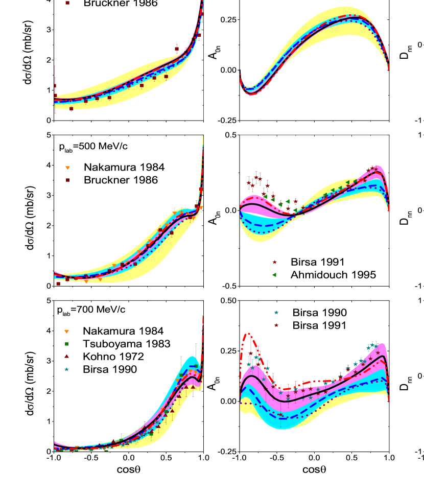
Figure 12: Differential cross sections, analyzing powers and spin correlation parameters $D_{nn}$ for charge-exchange scattering. For notations, see Fig. 10. Data are taken from Refs. [85, 71, 86, 80, 87] (differential cross sections), [88, 89, 87]. (analyzing powers), and [89] ($D_{nn}$). Note that the data for $A_{on}$ are for $546$ and $656$ MeV/c, respectively.

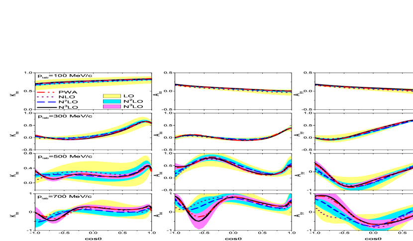
Figure 13: Spin correlation parameters $K_{nn}$, $A_{xx}$, $A_{yy}$, and $A_{zz}$ for charge-exchange scattering. For notations, see Fig. 10.

Also with regard to the analyzing power $A_{on}$ the uncertainty bands look similar to the pattern one observes in $Nd$ scattering. As already said above, for spin-dependent observables higher partial waves play a more important role and the uncertainty in their reproduction is also reflected more prominently in the results for the observables. Interestingly, the uncertainty exhibits a strong angular dependence. It seems that the angles where it is small are strongly correlated with the zeros of specific Legendre polynomials where then the contributions of, say, $D$-waves are zero and likewise their contribution to the uncertainty. For $A_{on}$ and also for other spin-dependent observables there is a visible difference between our N³LO results (solid curve) and the PWA (dash-dotted curve) at the highest energy displayed in Figs. 10 and 11.

Differential cross sections, analyzing powers and the spin-correlation parameters $D_{nn}$ for the charge-exchange reaction $\bar{p}p\to\bar{n}n$ are shown in Fig. 12. Results for further spin-dependent observables can be found in Fig. 13. The quality of the reproduction of the PWA results by our EFT interaction at N³LO but also the convergence properties with increasing order and the uncertainties are similar to those observed for $\bar{p}p$ elastic scattering. However, visible deviations from the PWA start already at somewhat smaller energies. This is most obvious in case of the analyzing power $A_{on}$ where noticeable differences of our N³LO results to those of the PWA occur already from $p_{\rm lab}\sim 500\,$MeV ($T_{\rm lab}\sim 125\,$MeV) onwards, cf. Fig. 12. Note that the lowest momentum is very close to the $\bar{n}n$ threshold, which is at $p_{\rm lab}=98.70\,$MeV, so that the kinetic energy in the $\bar{n}n$ system is only of the order of a few keV. Despite of that the spin-dependent observables exhibit already a distinct angular dependence and $A_{on}$ is clearly nonzero.

In any case, overall we can conclude that chiral EFT at N³LO not only allows for an excellent reproduction of the PWA results but also of the actual observables for energies below $p_{\rm lab}\sim 500\,$MeV ($T_{\rm lab}\sim 125\,$MeV) and it still provides a good description of the data at energies of the order of $p_{\rm lab}\sim 700\,$MeV ($T_{\rm lab}\sim 230\,$MeV)

5 Predictions

The lowest momentum for which results of the PWA are provided in Ref. [32], and accordingly are taken into account in our fitting procedure, is $p_{lab}=100$ MeV/c corresponding to $T_{lab}=5.32$ MeV. As can be seen in Table III of Ref. [32] no data below $100$ MeV/c have been included in the analysis, and only a few below $200$ MeV/c. In view of this we consider results of our $\bar{N}N$ potential at momenta below $100$ MeV/c as genuine predictions. First of all this concerns the low-energy structure of the amplitudes given in terms of the effective range expansion. Results for the scattering lengths (for ${}^{1}S_{0}$ and ${}^{3}S_{1}$) and for scattering volumes (for the $P$ waves) are summarized in Table 3. These are complex numbers because of the presence of annihilation. The pertinent calculations were done in the isospin basis and the isospin $I$ is included here in the spectral notation, i.e. we write ${}^{(2I+1)(2S+1)}L_{J}$. As one can see in Table 3 the results for the ${}^{1}S_{0}$ partial waves are very stable and change very little with increasing order. There is a slightly larger variation in case of the ${}^{3}S_{1}$. Somewhat stronger variations occur in the $P$ waves where those in the ${}^{3}P_{2}$ partial waves are by far the most dramatic ones. This is not surprising in view of the coupling of the ${}^{3}P_{2}$ to the ${}^{3}F_{2}$ and the fact that there is only a single (but complex-valued) LEC at NLO and N²LO that can be used in the fit to the ${}^{3}P_{2}$ and ${}^{3}F_{2}$ phase shifts and the mixing angle $\epsilon_{2}$.

Table 3: Scattering lengths and volumes for different partial waves for the chiral potentials with $R=0.9$ fm. $\bar{a}^{cs}_{S,\bar{p}p}$ and $\bar{a}^{cs}_{P,\bar{p}p}$ are spin-averaged results obtained from a calculation in particle basis including the Coulomb force. For comparison N²LO predictions of our previous chiral potential are included, based on the cutoff combination ($\Lambda$, $\tilde{\Lambda}$) = (450,500) MeV [42].

	NLO	N2LO	N3LO	N2LO [42]
$a_{{}^{11}S_{0}}$ (fm)	$-$0.21 $-$ i 1.20	$-$0.21 $-$ i 1.22	$-$0.20 $-$ i 1.23	$-$0.21 $-$ i1.21
$a_{{}^{31}S_{0}}$ (fm)	1.06 $-$ i 0.57	1.05 $-$ i 0.60	1.05 $-$ i 0.58	1.03 $-$ i0.58
$a_{{}^{13}S_{1}}$ (fm)	1.33 $-$ i 0.85	1.39 $-$ i 0.89	1.42 $-$ i 0.88	1.37 $-$ i0.88
$a_{{}^{33}S_{1}}$ (fm)	0.44 $-$ i 0.92	0.45 $-$ i 0.95	0.44 $-$ i 0.96	0.44 $-$ i0.91
$a_{{}^{13}P_{0}}$ (fm3)	$-$3.62 $-$ i 8.05	$-$3.18 $-$ i 8.02	$-$2.83 $-$ i 7.82	$-$3.76 $-$ i7.16
$a_{{}^{33}P_{0}}$ (fm3)	2.22 $-$ i 0.31	2.16 $-$ i 0.32	2.18 $-$ i 0.19	2.36 $-$ i1.14
$a_{{}^{11}P_{1}}$ (fm3)	$-$2.72 $-$ i 0.34	$-$2.76 $-$ i 0.35	$-$2.87 $-$ i 0.36	$-$2.87 $-$ i0.25
$a_{{}^{31}P_{1}}$ (fm3)	0.97 $-$ i 0.29	0.87 $-$ i 0.31	0.80 $-$ i 0.34	0.86 $-$ i0.20
$a_{{}^{13}P_{1}}$ (fm3)	4.65 $-$ i 0.07	4.60 $-$ i 0.07	4.61 $-$ i 0.05	4.77 $-$ i0.02
$a_{{}^{33}P_{1}}$ (fm3)	$-$1.81 $-$ i 0.47	$-$1.92 $-$ i 0.50	$-$2.04 $-$ i 0.55	$-$2.02 $-$ i0.39
$a_{{}^{13}P_{2}}$ (fm3)	$-$0.42 $-$ i 0.96	$-$0.55 $-$ i 1.03	$-$0.74 $-$ i 1.13	$-$0.45 $-$ i0.57
$a_{{}^{33}P_{2}}$ (fm3)	$-$0.29 $-$ i 0.37	$-$0.38 $-$ i 0.38	$-$0.48 $-$ i 0.34	$-$0.28 $-$ i0.23
$\bar{a}^{cs}_{S,\bar{p}p}$ (fm)	0.78 $-$ i 0.71	0.80 - i 0.73	0.80 $-$ i 0.74	0.79 $-$ i 0.72
$\bar{a}^{cs}_{P,\bar{p}p}$ (fm3)	$-$0.05 $-$ i0.74	$-$0.12 - i 0.77	$-$0.19 $-$ i 0.77	$-$0.10 $-$ i0.55

Table 3 contains also scattering lengths and volumes predicted in our earlier study of the $\bar{N}N$ interaction within chiral EFT based on a momentum-space cutoff [42]. We include here the results at N²LO and for the cutoff combination ($\Lambda$,$\tilde{\Lambda}$) = ($450$,$500$) MeV. It is reassuring to see that in most partial waves the predictions are very similar or even identical. More noticeable differences occur only in $P$ waves, and in particular in the ${}^{3}P_{2}$ – for the reasons just discussed.

There is some experimental information that puts constraints on these scattering lengths. Measurements of the level shifts and widths of antiproton-proton atoms have been used to infer values for the spin-averaged $\bar{p}p$ scattering lengths. Corresponding results can be found in Ref. [90], together with values for the imaginary part of the scattering lengths that are deduced from measurements of the $\bar{n}p$ annihilation cross section in combination with the ones for $\bar{p}p$ annihilation. Here we prefer to compare our predictions directly with the measured level shifts and widths [91, 92, 93, 94], see Table 4. For that the Trueman formula [95] was applied to the theory results with the second-order term taken into account for the $S$-waves. It has been found in Ref. [96] that values obtained in this way agree rather well with direct calculations. In this context let us recall that the results in Table 4, including those for the N²LO interaction from Ref. [42], are deduced, of course, from a calculation in particle basis. In particular, the Coulomb force in $\bar{p}p$ is taken into account and likewise the $p$-$n$ mass difference that leads to separated thresholds for the $\bar{p}p$ and $\bar{n}n$ channels. The corresponding results given in our earlier study of the $\bar{N}N$ interaction within chiral EFT [42] are from a calculation in the isospin basis.

Experimental evidence on level shifts and widths in antiprotonic hydrogen was not taken into account in the PWA [32]. Anyway, it should be said that additional assumptions have to be made in order to derive the splitting of the ${}^{1}S_{0}$ and ${}^{3}S_{1}$ level shifts from the experiment [94, 97]. This caveat has to be kept in mind when comparing the theory results with experiments. Notwithstanding, there is a remarkable agreement between our predictions and the experimental values, with the only exception being the level shift in the ${}^{3}P_{0}$ partial wave.

Table 4: Hadronic shifts and broadenings in hyperfine states of $\bar{p}$H for the chiral potentials with $R=0.9$ fm. For comparison N²LO predictions of our previous chiral potential are included, based on the cutoff combination ($\Lambda$, $\tilde{\Lambda}$) = (450,500) MeV [42]. The experimental information is taken from Refs. [91, 93, 92, 94].

	NLO	N2LO	N3LO	N2LO [42]	Experiment
$E_{{}^{1}S_{0}}$ (eV)	$-$448	$-$446	$-$443	$-$436	$-$440(75) [92]
					$-$740(150) [91]
$\Gamma_{{}^{1}S_{0}}$ (eV)	1155	1183	1171	1174	1200(250) [92]
					1600(400) [91]
$E_{{}^{3}S_{1}}$ (eV)	$-$742	$-$766	$-$770	$-$756	$-$785(35) [92]
					$-$850(42) [93]
$\Gamma_{{}^{3}S_{1}}$ (eV)	1106	1136	1161	1120	940(80) [92]
					770(150) [93]
$E_{{}^{3}P_{0}}$ (meV)	17	12	8	16	139(28) [94]
$\Gamma_{{}^{3}P_{0}}$ (meV)	194	195	188	169	120(25) [94]
$E_{1S}$ (eV)	$-$670	$-$688	$-$690	$-$676	$-$721(14) [92]
$\Gamma_{1S}$ (eV)	1118	1148	1164	1134	1097(42) [92]
$E_{2P}$ (meV)	1.3	2.8	4.7	2.3	15(20) [94]
$\Gamma_{2P}$ (meV)	36.2	37.4	37.9	27	38.0(2.8) [94]

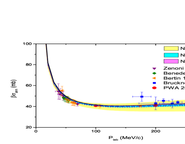
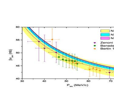
Figure 14: $\bar{p}p$ annihilation cross section multiplied by the velocity $\beta$ of the incoming $\bar{p}$. For notations, see Fig. 9. The results of the PWA [32] are indicated by circles. Data are taken from [98, 99, 100, 101].

There are measurements of the $\bar{p}p$ annihilation cross section at very low energy [98, 99, 100, 101]. Also those experiments were not taken into account in the PWA [32]. We present our predictions for this observable in Fig. 14, where the annihilation cross section multiplied by the velocity $\beta$ of the incoming $\bar{p}$ is shown. Results based on the amplitudes of the PWA are also included (filled circles). An interesting aspects of those data is that one can see the anomalous behavior of the reaction cross section near threshold due to the presence of the attractive Coulomb force [102]. Usually the cross sections for exothermic reactions behave like $1/\beta$ so that $\beta\sigma_{ann}$ is then practically constant, cf. Fig. 14 for $p_{lab}\approx 100-300$ MeV/c. However, the Coulomb attraction modifies that to a $1/\beta^{2}$ behavior for energies very close to the threshold.

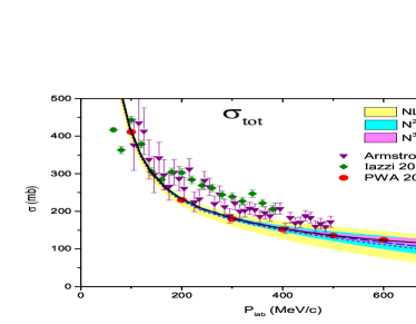
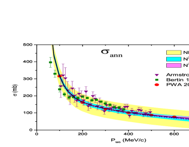
Figure 15: Total ($\sigma_{tot}$) and integrated annihilation ($\sigma_{ann}$) cross sections for $\bar{n}p$ scattering. For notations, see Fig. 9. Data are taken from Refs. [103, 104, 105].

Finally, for illustration we show our predictions for $\bar{n}p$ scattering, see Fig. 15. The $\bar{n}p$ system is a pure isospin $I=1$ state so that one can test the $I=1$ component of the $\bar{N}N$ amplitude independently. Note that the PWA results displayed in Fig. 15 include again partial-wave amplitudes from our N³LO interaction for $J\geq 5$. However, for integrated cross sections the contributions of those higher partial waves is really very small, even at $p_{lab}=800$ MeV/c.

6 Summary

In Ref. [38] a new generation of $NN$ potentials derived in the framework of chiral effective field theory was presented. In that work a new local regularization scheme was introduced and applied to the pion-exchange contributions of the $NN$ force. Furthermore, an alternative scheme for estimating the uncertainty was proposed that no longer depends on a variation of the cutoffs. In the present paper we adopted their suggestions and applied them in a study of the $\bar{N}N$ interaction. Specifically, a $\bar{N}N$ potential has been derived up to N³LO in the perturbative expansion, thereby extending a previous work by our group that had considered the $\bar{N}N$ force up to N²LO [42]. Like before, the pertinent low-energy constants have been fixed by a fit to the phase shifts and inelasticities provided by a recently published phase-shift analysis of $\bar{p}p$ scattering data [32].

We could show that an excellent reproduction of the $\bar{N}N$ amplitudes can be achieved at N³LO. Indeed, in many aspects the quality of the description is comparable to that one has found in case of the $NN$ interaction at the same order [38]. To be more specific, for the $S$-waves excellent agreement with the phase shifts and inelasticities of [32] has been obtained up to laboratory energies of about $300$ MeV, i.e. over the whole energy range considered. The same is also the case for most $P$-waves. Even many of the $D$-waves are described well up to $200$ MeV or beyond. Because of the overall quality in the reproduction of the individual partial waves there is also a nice agreement on the level of $\bar{N}N$ observables. Total and integrated elastic ($\bar{p}p\to\bar{p}p$) and charge-exchange ($\bar{p}p\to\bar{n}n$) cross sections agree well with the PWA results up to the highest energy considered while differential observables (cross sections, analyzing powers, etc.) are reproduced quantitatively up to $200$-$250$ MeV. Furthermore, and equally important, in most of the considered cases the achieved results agree with the ones based on the PWA within the estimated theoretical accuracy. Thus, the scheme for quantifying the uncertainty suggested in Ref. [38] seems to work well and can be applied reliably to the $\bar{N}N$ interaction as well. Finally, the low-energy representation of the $\bar{N}N$ amplitudes derived from chiral EFT compares well with the constraints derived from the phenomenology of antiprotonic hydrogen.

Appendix A The chiral potential up to N³LO

The one-pion exchange potential (OPEP) is given in Eq. (1). Up to N³LO, the chiral expansion of the two-pion exchange potential (TPEP) can be found in Refs. [37, 38, 106]. For the reader’s convenience we summarize the expressions below. The TPEP can be written in the form

$$V_{2\pi} = V_{C}+\mbox{\boldmath$\tau$}_{1}\cdot\mbox{\boldmath$\tau$}_{2}\,W_{C}+\left[V_{S}+\mbox{\boldmath$\tau$}_{1}\cdot\mbox{\boldmath$\tau$}_{2}\,W_{S}\right]\,\mbox{\boldmath$\sigma$}_{1}\cdot\mbox{\boldmath$\sigma$}_{2}+\left[V_{T}+\mbox{\boldmath$\tau$}_{1}\cdot\mbox{\boldmath$\tau$}_{2}\,W_{T}\right]\,\mbox{\boldmath$\sigma$}_{1}\cdot\mbox{\boldmath$q$}\,\mbox{\boldmath$\sigma$}_{2}\cdot\mbox{\boldmath$q$}$$ (A.1)

$$+ \left[V_{LS}+\mbox{\boldmath$\tau$}_{1}\cdot\mbox{\boldmath$\tau$}_{2}\,W_{LS}\right]\,i(\mbox{\boldmath$\sigma$}_{1}+\mbox{\boldmath$\sigma$}_{2})\cdot(\mbox{\boldmath$q$}\times\mbox{\boldmath$k$})\,,$$

where ${\mbox{\boldmath$q$}}={\mbox{\boldmath$p$}}^{\prime}-{\mbox{\boldmath$p$}}$, ${\mbox{\boldmath$k$}}=({\mbox{\boldmath$p$}}^{\prime}+{\mbox{\boldmath$p$}})/2$, and $\mbox{\boldmath$\tau$}_{i}$ is the isospin Pauli matrix associated with the nucleon (antinucleon) $i$. $V$ denotes the isoscalar part and $W$ the isovector part where the subscripts $C$, $S$, $T$, $LS$ refer to the central, spin-spin, tensor, and spin-orbit terms, respectively. Each component of $V$ and $W$ is given by a sum $V=V^{(0)}+V^{(2)}+V^{(3)}+V^{(4)}$ (analogous for $W$) where the superscript in the bracket refers to the chiral dimension. The order-$Q^{2}$ contributions take the form

$$W_{C}^{(2)} = -\frac{L(q)}{384\pi^{2}F_{\pi}^{4}}\bigg{[}4M_{\pi}^{2}(5g_{A}^{4}-4g_{A}^{2}-1)+q^{2}(23g_{A}^{4}-10g_{A}^{2}-1)+\frac{48g_{A}^{4}M_{\pi}^{4}}{4M_{\pi}^{2}+q^{2}}\bigg{]}\,,$$

$$V_{T}^{(2)} = -\frac{1}{q^{2}}V_{S}^{(2)}=-\frac{3g_{A}^{4}}{64\pi^{2}F_{\pi}^{4}}\,L(q)\,,$$

$$V_{C}^{(2)} = V_{LS}^{(2)}=W_{S}^{(2)}=W_{T}^{(2)}=W_{LS}^{(2)}=0\,.$$ (A.2)

The loop function $L(q)$ is defined in dimensional regularization (DR) via

$$L(q)=\frac{\sqrt{4M_{\pi}^{2}+q^{2}}}{q}\ln\frac{\sqrt{4M_{\pi}^{2}+q^{2}}+q}{2M_{\pi}}\,.$$ (A.3)

Notice that all polynomial terms are absorbed into contact interactions, as given in Eqs. (2)-(LABEL:VC). The corrections at order $Q^{3}$ giving rise to the subleading TPEP have the form

$$V_{C}^{(3)} = -\frac{3g_{A}^{2}}{16\pi F_{\pi}^{4}}\bigg{[}2M_{\pi}^{2}(2c_{1}-c_{3})-c_{3}q^{2}\bigg{]}(2M_{\pi}^{2}+q^{2})A(q)\,,$$

$$W_{T}^{(3)} = -\frac{1}{q^{2}}W_{S}^{(3)}=-\frac{g_{A}^{2}}{32\pi F_{\pi}^{4}}\,c_{4}(4M_{\pi}^{2}+q^{2})A(q)\,,$$

$$V_{S}^{(3)} = V_{T}^{(3)}=V_{LS}^{(3)}=W_{C}^{(3)}=W_{LS}^{(3)}=0\,,$$ (A.4)

where the loop function $A(q)$ is given in DR by

$$A(q)=\frac{1}{2q}\arctan\frac{q}{2M_{\pi}}\,.$$ (A.5)

At order $Q^{4}$, i.e. N³LO, the contributions of one-loop “bubble” diagrams to the TPEP are

$$V_{C}^{(4)} = \frac{3}{16\pi^{2}F_{\pi}^{4}}\,L(q)\,\left\{\left[\frac{c_{2}}{6}(4M_{\pi}^{2}+q^{2})+c_{3}(2M_{\pi}^{2}+q^{2})-4c_{1}M_{\pi}^{2}\right]^{2}+\frac{c_{2}^{2}}{45}(4M_{\pi}^{2}+q^{2})^{2}\right\}\,,$$

$$W_{T}^{(4)} = -\frac{1}{q^{2}}W_{S}^{(4)}=\frac{c_{4}^{2}}{96\pi^{2}F_{\pi}^{4}}(4M_{\pi}^{2}+q^{2})\,L(q)\,.$$ (A.6)

Since the regularization is done in coordinate space the potentials have to be Fourier transformed. For the contributions above this can be done analytically and the corresponding expressions (up to N²LO) have been given in [107, 108].

$$\noindent W_{S}^{(0)}(r) = \frac{g_{A}^{2}x^{2}e^{-x}}{48\pi F_{\pi}^{2}r^{3}}\;,$$ (A.7)

$$\noindent\tilde{W}_{T}^{(0)}(r) = \frac{g_{A}^{2}e^{-x}(x^{2}+3x+3)}{48\pi F_{\pi}^{2}r^{3}}\;,$$ (A.8)

$$\noindent V_{S}^{(2)}(r) = \frac{g_{A}^{4}x\left((2x^{2}+3)K_{1}(2x)+3xK_{0}(2x)\right)}{32\pi^{3}F_{\pi}^{4}r^{5}}\;,$$ (A.9)

$$\noindent\tilde{V}_{T}^{(2)}(r) = -\frac{g_{A}^{4}x\left((4x^{2}+15)K_{1}(2x)+12xK_{0}(2x)\right)}{128\pi^{3}F_{\pi}^{4}r^{5}}\;,$$ (A.10)

$$\noindent W_{C}^{(2)}(r) = -\frac{x\left(x\left(g_{A}^{4}(4x^{2}+23)-10g_{A}^{2}-1\right)K_{0}(2x)+\left(g_{A}^{4}(12x^{2}+23)-2g_{A}^{2}(2x^{2}+5)-1\right)K_{1}(2x)\right)}{128\pi^{3}F_{\pi}^{4}r^{5}}\;,$$ (A.11)

$$\noindent V_{C}^{(3)}(r) = \frac{3g_{A}^{2}e^{-2x}\left(2c_{1}x^{2}(x+1)^{2}+c_{3}(x^{4}+4x^{3}+10x^{2}+12x+6)\right)}{32\pi^{2}F_{\pi}^{4}r^{6}}\;,$$ (A.12)

$$\noindent W_{S}^{(3)}(r) = \frac{c_{4}g_{A}^{2}e^{-2x}(x+1)(2x^{2}+3x+3)}{48\pi^{2}F_{\pi}^{4}r^{6}}\;,$$ (A.13)

$$\noindent\tilde{W}_{T}^{(3)}(r) = -\frac{c_{4}g_{A}^{2}e^{-2x}(x+1)(x^{2}+3x+3)}{48\pi^{2}F_{\pi}^{4}r^{6}}\;,$$ (A.14)

where $x=M_{\pi}r$, $K_{i}(x)$ is the modified Bessel function of the second kind and the superscript in the bracket refers to the chiral dimension. Note that the tensor parts of the potentials in coordinate space ($\tilde{V}_{T}$, $\tilde{W}_{T}$) are written with a tilde as a reminder that they are defined in terms of the irreducible tensor operator $S_{12}=3(\mbox{\boldmath$\sigma$}_{1}\cdot\mbox{\boldmath$\hat{r}$}\,\mbox{\boldmath$\sigma$}_{2}\cdot\mbox{\boldmath$\hat{r}$})-\mbox{\boldmath$\sigma$}_{1}\cdot\mbox{\boldmath$\sigma$}_{2}$ where $\mbox{\boldmath$\hat{r}$}=\mbox{\boldmath$r$}/r$.

The relativistic, i.e. the $1/m$, corrections are given by

$$\noindent V_{C,m}^{(4)}(r) = \frac{3g_{A}^{4}e^{-2x}(x^{5}+10x^{4}+28x^{3}+46x^{2}+48x+24)}{1024\pi^{2}F_{\pi}^{4}mr^{6}}\;,$$ (A.15)

$$\noindent V_{S,m}^{(4)}(r) = -\frac{g_{A}^{4}e^{-2x}(6x^{4}+22x^{3}+43x^{2}+48x+24)}{512\pi^{2}F_{\pi}^{4}mr^{6}}\;,$$ (A.16)

$$\noindent\tilde{V}_{T,m}^{(4)}(r) = \frac{g_{A}^{4}e^{-2x}(6x^{4}+31x^{3}+76x^{2}+96x+48)}{1024\pi^{2}F_{\pi}^{4}mr^{6}}\;,$$ (A.17)

$$\noindent V_{LS,m}^{(4)}(r) = -\frac{3g_{A}^{4}e^{-2x}(x+1)(x^{2}+2x+2)}{64\pi^{2}F_{\pi}^{4}mr^{6}}\;,$$ (A.18)

$$\noindent W_{C,m}^{(4)}(r) = \frac{g_{A}^{2}e^{-2x}\left(g_{A}^{2}(3x^{5}+10x^{4}+36x^{3}+82x^{2}+96x+48)-4(x^{4}+4x^{3}+10x^{2}+12x+6)\right)}{512\pi^{2}F_{\pi}^{4}mr^{6}}\;,$$ (A.19)

$$\noindent W_{S,m}^{(4)}(r) = -\frac{g_{A}^{2}e^{-2x}\left(g_{A}^{2}(2x^{4}+10x^{3}+21x^{2}+24x+12)-4(2x^{3}+5x^{2}+6x+3)\right)}{768\pi^{2}F_{\pi}^{4}mr^{6}}\;,$$ (A.20)

$$\noindent\tilde{W}_{T,m}^{(4)}(r) = \frac{g_{A}^{2}e^{-2x}\left(g_{A}^{2}(2x^{4}+13x^{3}+36x^{2}+48x+24)-8(x^{3}+4x^{2}+6x+3)\right)}{1536\pi^{2}F_{\pi}^{4}mr^{6}}\;,$$ (A.21)

$$\noindent W_{LS,m}^{(4)}(r) = \frac{g_{A}^{2}(g_{A}^{2}-1)e^{-2x}(x+1)^{2}}{32\pi^{2}F_{\pi}^{4}mr^{6}}\;.$$ (A.22)

The subleading order corrections to the $\pi N$ vertex are given by

$$\noindent V_{C,sl}^{(4)}(r) = -\frac{g_{A}^{2}x}{128\pi^{3}F_{\pi}^{4}mr^{7}}\left[K_{0}(2x)\left(48x^{3}(6c_{1}+c_{2}-3c_{3})+24x^{5}(2c_{1}+c_{3})-48x(c_{2}-6c_{3})(2x^{2}+5)\right)\right.$$ (A.23)

$$-2K_{1}(2x)\left(-16x^{4}(6c_{1}+c_{2}-3c_{3})-24x^{2}(6c_{1}+c_{2}-3c_{3})+6x^{4}(c_{2}-2c_{3})\right.$$

$$+\left.\left.4(c_{2}-6c_{3})(4x^{4}+27x^{2}+30)\right)\right]\;,$$

$$\noindent V_{LS,sl}^{(4)}(r) = \frac{3c_{2}g_{A}^{2}x\left((2x^{2}+5)K_{1}(2x)+5xK_{0}(2x)\right)}{8\pi^{3}F_{\pi}^{4}mr^{7}}\;,$$ (A.24)

$$\noindent W_{C,sl}^{(4)}(r) = \frac{c_{4}x\left(2x\left(g_{A}^{2}(8x^{2}+25)+x^{2}+5\right)K_{0}(2x)+\left(g_{A}^{2}(4x^{4}+41x^{2}+50)+7x^{2}+10\right)K_{1}(2x)\right)}{32\pi^{3}F_{\pi}^{4}mr^{7}}\;,$$ (A.25)

$$\noindent W_{S,sl}^{(4)}(r) = -\frac{c_{4}x\left(x\left(g_{A}^{2}(4x^{2}+35)-5\right)K_{1}(2x)+2\left(5g_{A}^{2}(2x^{2}+7)-x^{2}-5\right)\left(xK_{0}(2x)+K_{1}(2x)\right)\right)}{48\pi^{3}F_{\pi}^{4}mr^{7}}\;,$$ (A.26)

$$\noindent\tilde{W}_{T,sl}^{(4)}(r) = \frac{c_{4}x\left(2x\left(g_{A}^{2}(4x^{2}+59)-8\right)K_{1}(2x)+\left(g_{A}^{2}(52x^{2}+245)-4x^{2}-35\right)\left(xK_{0}(2x)+K_{1}(2x)\right)\right)}{192\pi^{3}F_{\pi}^{4}mr^{7}}\;,$$ (A.27)

$$\noindent W_{LS,sl}^{(4)}(r) = -\frac{c_{4}x\left(x\left(g_{A}^{2}(4x^{2}+25)+5\right)K_{0}(2x)+\left(g_{A}^{2}(16x^{2}+25)+2x^{2}+5\right)K_{1}(2x)\right)}{16\pi^{3}F_{\pi}^{4}mr^{7}}\;.$$ (A.28)

The one loop ‘bubble’ diagrams corrections to the TPEP potential amount to

$$\noindent V_{C,b}^{(4)}(r) = -\frac{3x}{32\pi^{3}F_{\pi}^{4}r^{7}}\left[K_{1}(2x)\left(4\left(4c_{1}^{2}x^{4}+4c_{1}c_{3}x^{2}(x^{2}+3)+c_{3}^{2}(x^{4}+21x^{2}+30)\right)\right.\right.$$ (A.29)

$$\left.+8c_{2}\left(c_{1}x^{2}+c_{3}(3x^{2}+5)\right)+3c_{2}^{2}(x^{2}+2)\right)$$

$$\left.+2xK_{0}(2x)\left(2c_{2}(2c_{1}x^{2}+c_{3}x^{2}+10c_{3})+12c_{3}(2c_{1}x^{2}+c_{3}x^{2}+5c_{3})+3c_{2}^{2}\right)\right]\;,$$

$$\noindent W_{S,b}^{(4)}(r) = \frac{c_{4}^{2}x\left(2x(x^{2}+5)K_{0}(2x)+(7x^{2}+10)K_{1}(2x)\right)}{24\pi^{3}F_{\pi}^{4}r^{7}}\;,$$ (A.30)

$$\noindent\tilde{W}_{T,b}^{(4)}(r) = -\frac{c_{4}^{2}x\left(x(4x^{2}+35)K_{0}(2x)+5(4x^{2}+7)K_{1}(2x)\right)}{96\pi^{3}F_{\pi}^{4}r^{7}}\;.$$ (A.31)

There are further contributions to the TPEP at N³LO where one cannot get analytical forms in coordinate space. Most conveniently one can write those in the (subtracted) spectral representation

$$V_{C,S}(q) = -\frac{2q^{6}}{\pi}\int_{2M_{\pi}}^{\infty}\,d\mu\frac{\rho_{C,S}(\mu)}{\mu^{5}(\mu^{2}+q^{2})}\,,\quad\quad V_{T}(q)=\frac{2q^{4}}{\pi}\int_{2M_{\pi}}^{\infty}\,d\mu\frac{\rho_{T}(\mu)}{\mu^{3}(\mu^{2}+q^{2})}\,,$$

$$W_{C,S}(q) = -\frac{2q^{6}}{\pi}\int_{2M_{\pi}}^{\infty}\,d\mu\frac{\eta_{C,S}(\mu)}{\mu^{5}(\mu^{2}+q^{2})}\,,\quad\quad W_{T}(q)=\frac{2q^{4}}{\pi}\int_{2M_{\pi}}^{\infty}\,d\mu\frac{\eta_{T}(\mu)}{\mu^{3}(\mu^{2}+q^{2})}\,,$$ (A.32)

where $\rho_{i}$ and $\eta_{i}$ denote the corresponding spectral functions which are related to the potential via $\rho_{i}(\mu)={\rm Im}V_{i}(i\mu)$, $\eta_{i}(\mu)={\rm Im}W_{i}(i\mu)$. For the spectral functions $\rho_{i}(\mu)$ ($\eta_{i}(\mu)$) one finds [106]:

$$\rho_{C}^{(4)}(\mu) = -\frac{3g_{A}^{4}(\mu^{2}-2M_{\pi}^{2})}{\pi\mu(4F_{\pi})^{6}}\,\bigg{\{}(M_{\pi}^{2}-2\mu^{2})\bigg{[}2M_{\pi}+\frac{2M_{\pi}^{2}-\mu^{2}}{2\mu}\ln\frac{\mu+2M_{\pi}}{\mu-2M_{\pi}}\bigg{]}+4g_{A}^{2}M_{\pi}(2M_{\pi}^{2}-\mu^{2})\bigg{\}}\,,$$

$$\eta_{S}^{(4)}(\mu) = \mu^{2}\eta_{T}^{(4)}(\mu)=-\frac{g_{A}^{4}(\mu^{2}-4M_{\pi}^{2})}{\pi(4F_{\pi})^{6}}\,\left\{\left(M_{\pi}^{2}-\frac{\mu^{2}}{4}\right)\ln\frac{\mu+2M_{\pi}}{\mu-2M_{\pi}}+(1+2g_{A}^{2})\mu M_{\pi}\right\}\,,$$

$$\rho_{S}^{(4)}(\mu) = \mu^{2}\rho_{T}^{(4)}(\mu)=-\left\{\frac{g_{A}^{2}r^{3}\mu}{8F_{\pi}^{4}\pi}(\bar{d}_{14}-\bar{d}_{15})-\frac{2g_{A}^{6}\mu r^{3}}{(8\pi F_{\pi}^{2})^{3}}\left[\frac{1}{9}-J_{1}+J_{2}\right]\right\}\,,$$

$$\eta_{C}^{(4)}(\mu) = \Bigg{\{}\frac{rt^{2}}{24F_{\pi}^{4}\mu\pi}\left[2(g_{A}^{2}-1)r^{2}-3g_{A}^{2}t^{2}\right](\bar{d}_{1}+\bar{d}_{2})$$ (A.33)

$${}+\frac{r^{3}}{60F_{\pi}^{4}\mu\pi}\left[6(g_{A}^{2}-1)r^{2}-5g_{A}^{2}t^{2}\right]\bar{d}_{3}-\frac{rM_{\pi}^{2}}{6F_{\pi}^{4}\mu\pi}\left[2(g_{A}^{2}-1)r^{2}-3g_{A}^{2}t^{2}\right]\bar{d}_{5}$$

$${}-\frac{1}{92160F_{\pi}^{6}\mu^{2}\pi^{3}}\Big{[}-320(1+2g_{A}^{2})^{2}M_{\pi}^{6}+240(1+6g_{A}^{2}+8g_{A}^{4})M_{\pi}^{4}\mu^{2}$$

$${}\mbox{\hskip 85.35826pt}-60g_{A}^{2}(8+15g_{A}^{2})M_{\pi}^{2}\mu^{4}+(-4+29g_{A}^{2}+122g_{A}^{4}+3g_{A}^{6})\mu^{6}\Big{]}\ln\frac{2r+\mu}{2M_{\pi}}$$

$${}-\frac{r}{2700\mu(8\pi F_{\pi}^{2})^{3}}\Big{[}-16(171+2g_{A}^{2}(1+g_{A}^{2})(327+49g_{A}^{2}))M_{\pi}^{4}$$

$${}\mbox{\hskip 85.35826pt}+4(-73+1748g_{A}^{2}+2549g_{A}^{4}+726g_{A}^{6})M_{\pi}^{2}\mu^{2}$$

$${}\mbox{\hskip 85.35826pt}-(-64+389g_{A}^{2}+1782g_{A}^{4}+1093g_{A}^{6})\mu^{4}\Big{]}$$

$${}+\frac{2r}{3\mu(8\pi F_{\pi}^{2})^{3}}\Big{[}g_{A}^{6}t^{4}J_{1}-2g_{A}^{4}(2g_{A}^{2}-1)r^{2}t^{2}J_{2}\Big{]}\Bigg{\}}\,,$$

where the abbreviations are

$$r=\frac{1}{2}\sqrt{\mu^{2}-4M_{\pi}^{2}}\,,\quad\quad\quad t=\sqrt{\mu^{2}-2M_{\pi}^{2}}\,,$$ (A.34)

and

$$J_{1} = \int_{0}^{1}\,dx\,\bigg{\{}\frac{M_{\pi}^{2}}{r^{2}x^{2}}-\bigg{(}1+\frac{M_{\pi}^{2}}{r^{2}x^{2}}\bigg{)}^{3/2}\ln\frac{rx+\sqrt{M_{\pi}^{2}+r^{2}x^{2}}}{M_{\pi}}\bigg{\}}\,,$$

$$J_{2} = \int_{0}^{1}\,dx\,x^{2}\bigg{\{}\frac{M_{\pi}^{2}}{r^{2}x^{2}}-\bigg{(}1+\frac{M_{\pi}^{2}}{r^{2}x^{2}}\bigg{)}^{3/2}\ln\frac{rx+\sqrt{M_{\pi}^{2}+r^{2}x^{2}}}{M_{\pi}}\bigg{\}}\,.$$ (A.35)

The LECs $\bar{d}_{1},\;\bar{d}_{2},\;\bar{d}_{3},\;\bar{d}_{5},\;\bar{d}_{14}$ and $\bar{d}_{15}$ are discussed in Sec. 2.1. This part of the potential is Fourier transformed numerically.

After regularization in coordinate space, we need to transform the potential back to momentum space where we solve the Lippmann-Schwinger equation. For that we employ the master formulae given in Ref. [109] and obtain:

$$V_{C}(q) = 4\pi\int_{0}^{\infty}f(r)\,V_{C}(r)j_{0}(qr)r^{2}dr\;,$$

$$V_{S}(q) = 4\pi\int_{0}^{\infty}f(r)\,\left(V_{S}(r)j_{0}(qr)+\tilde{V}_{T}(r)j_{2}(qr)\right)r^{2}dr\;,$$

$$V_{T}(q) = -\frac{12\pi}{q^{2}}\int_{0}^{\infty}f(r)\,\tilde{V}_{T}(r)j_{2}(qr)r^{2}dr\;,$$

$$V_{SL}(q) = \frac{4\pi}{q}\int_{0}^{\infty}f(r)\,V_{LS}(r)j_{1}(qr)r^{3}dr\;,$$ (A.36)

Here $f(r)$ is the regulator function given in Eq. (33). The same relations apply also to the isovector part $W$.

Appendix B Values of the low-energy constants

Values of the LECs obtained in our fit to the $\bar{N}N$ phase shifts of the PWA [32] at N³LO are collected in Tables B.1 and B.2 for the cutoffs $R=0.8-1.2$ fm. Values of the LECs obtained in our fit to the $\bar{N}N$ phase shifts of the PWA [32] at LO, NLO, N²LO for the cutoffs $R=0.9$ fm and $R=1.0$ fm are collected in Table B.3.

LEC	R=0.8 fm	R=0.9 fm	R=1.0 fm	R=1.1 fm	R=1.2 fm
$\tilde{C}_{{}^{11}S_{0}}$ (GeV-2)	0.1816	0.0734	0.0293	0.0007	-0.0089
$C_{{}^{11}S_{0}}$ (GeV-4)	-0.2134	0.0032	0.1353	0.1754	0.2188
$D^{1}_{{}^{11}S_{0}}$ (GeV-6)	-2.8614	-3.8012	-4.5883	-3.7943	-0.0746
$D^{2}_{{}^{11}S_{0}}$ (GeV-8)	2.1256	2.2443	3.0715	4.5639	6.4500
$\tilde{C}^{a}_{{}^{11}S_{0}}$ (GeV-1)	-0.5809	-0.5437	-0.5326	-0.5173	-0.5007
$C^{a}_{{}^{11}S_{0}}$ (GeV-3)	0.5993	0.1067	-0.5747	-1.5894	-2.7102
$\tilde{C}_{{}^{31}S_{0}}$ (GeV-2)	0.3960	0.1870	0.1189	0.0889	0.0737
$C_{{}^{31}S_{0}}$ (GeV-4)	0.0966	-0.0702	-0.0796	-0.1356	-0.1228
$D^{1}_{{}^{31}S_{0}}$ (GeV-6)	2.8886	1.4143	-1.3774	-5.0372	-9.9353
$D^{2}_{{}^{31}S_{0}}$ (GeV-8)	1.4470	1.7541	3.2624	6.6055	9.9568
$\tilde{C}^{a}_{{}^{31}S_{0}}$ (GeV-1)	-0.5768	-0.5102	-0.5078	-0.5251	-0.5293
$C^{a}_{{}^{31}S_{0}}$ (GeV-3)	0.4809	0.3750	0.1227	-0.3239	-0.7031
$\tilde{C}_{{}^{13}S_{1}}$ (GeV-2)	1.6589	0.8795	0.5625	0.3402	0.2346
$C_{{}^{13}S_{1}}$ (GeV-4)	-1.4947	-1.3232	-1.2473	-1.2201	-1.3363
$D^{1}_{{}^{13}S_{1}}$ (GeV-6)	-1.0563	-4.1331	-8.2720	-13.3684	-22.8316
$D^{1}_{{}^{13}S_{1}}$ (GeV-8)	-2.3730	-5.0615	-8.3651	-13.4933	-17.9644
$\tilde{C}^{a}_{{}^{13}S_{1}}$ (GeV-1)	-1.1612	-0.9880	-0.9724	-1.0715	-1.0846
$C^{a}_{{}^{13}S_{1}}$ (GeV-3)	1.4455	1.8999	2.8473	4.0483	5.3069
$\tilde{C}_{{}^{33}S_{1}}$ (GeV-2)	0.2214	0.2537	0.2621	0.1740	0.0984
$C_{{}^{33}S_{1}}$ (GeV-4)	-0.8849	-0.7500	-0.1184	-0.0442	-0.0864
$D^{1}_{{}^{33}S_{1}}$ (GeV-6)	-0.9113	-2.5135	-3.1696	-2.5085	-0.2544
$D^{2}_{{}^{33}S_{1}}$ (GeV-8)	5.8826	7.0499	8.2400	9.5785	10.9252
$\tilde{C}^{a}_{{}^{33}S_{1}}$ (GeV-1)	1.7798	1.0938	0.7817	0.6102	0.5040
$C^{a}_{{}^{33}S_{1}}$ (GeV-3)	1.6053	2.0396	2.0031	2.3243	2.9964
$C_{{}^{1}\epsilon_{1}}$ (GeV-4)	-1.2873	-1.0422	-1.0352	-1.1118	-1.2042
$D^{1}_{{}^{1}\epsilon_{1}}$ (GeV-6)	1.5672	2.4207	3.1532	4.1075	4.9037
$D^{2}_{{}^{1}\epsilon_{1}}$ (GeV-8)	8.9117	9.0537	10.8574	14.7047	17.9407
$C^{a}_{{}^{1}\epsilon_{1}}$ (GeV-3)	-0.1132	-0.3203	-0.7550	-1.1708	-1.7234
$C_{{}^{3}\epsilon_{1}}$ (GeV-4)	-0.8700	-0.3729	-0.0271	0.1361	0.4158
$D^{1}_{{}^{3}\epsilon_{1}}$ (GeV-6)	0.0661	-0.4703	-2.3147	-6.4892	-9.1563
$D^{2}_{{}^{3}\epsilon_{1}}$ (GeV-8)	9.9717	9.9728	9.1269	9.9530	9.9987
$C^{a}_{{}^{3}\epsilon_{1}}$ (GeV-3)	0.5098	0.2399	-0.3413	-0.9511	-1.1465
$C_{{}^{13}P_{0}}$ (GeV-4)	-0.7131	-1.2874	-1.7249	-2.1000	-2.9288
$D^{1}_{{}^{13}P_{0}}$ (GeV-6)	0.8404	0.4728	-1.3347	-5.4425	-9.5526
$C^{a}_{{}^{13}P_{0}}$ (GeV-2)	-0.5149	-0.4760	-0.4338	-0.3411	-0.6103
$D^{a}_{{}^{13}P_{0}}$ (GeV-4)	-1.4175	-2.5931	-4.2633	-7.0558	-8.8683
$C_{{}^{33}P_{0}}$ (GeV-4)	-0.2927	-0.2364	-0.2263	-0.0486	0.1721
$D^{1}_{{}^{33}P_{0}}$ (GeV-6)	-0.4391	-1.8988	-3.6350	-6.7300	-10.8920
$C^{a}_{{}^{33}P_{0}}$ (GeV-2)	0.4600	0.4023	0.4034	0.3466	0.2792
$D^{a}_{{}^{33}P_{0}}$ (GeV-4)	0.6467	1.8980	3.5552	6.1373	9.6870
$C_{{}^{11}P_{1}}$ (GeV-4)	0.3393	0.3290	0.3235	0.1592	-0.0480
$D^{1}_{{}^{11}P_{1}}$ (GeV-6)	0.2221	1.2951	2.7015	5.1788	8.2461
$C^{a}_{{}^{11}P_{1}}$ (GeV-2)	-1.0467	-1.0598	-1.0268	-1.0098	-0.9880
$D^{a}_{{}^{11}P_{1}}$ (GeV-4)	-0.7349	-1.6834	-2.5470	-3.5875	-4.7692

Table B.1: Low-energy constants at N³LO for different cutoffs. The superscript $a$ indicates parameters that are related to the annihilation part, cf. Eqs. (17)-(22). Note that all parameters are in units of $10^{4}$.

LEC	R=0.8 fm	R=0.9 fm	R=1.0 fm	R=1.1 fm	R=1.2 fm
$C_{{}^{31}P_{1}}$ (GeV-4)	0.4044	0.2913	0.2541	0.0031	-0.2178
$D^{1}_{{}^{31}P_{1}}$ (GeV-6)	0.7746	2.1280	3.4240	5.9236	8.7283
$C^{a}_{{}^{31}P_{1}}$ (GeV-2)	-1.1010	-1.1208	-1.0835	-1.0868	-1.0770
$D^{a}_{{}^{31}P_{1}}$ (GeV-4)	-0.8621	-1.6859	-2.2918	-3.2685	-4.4792
$C_{{}^{13}P_{1}}$ (GeV-4)	-0.0481	0.0110	0.1200	0.3533	0.5733
$D^{1}_{{}^{13}P_{1}}$ (GeV-6)	-0.1271	-0.7636	-1.5221	-2.8235	-3.8502
$C^{a}_{{}^{13}P_{1}}$ (GeV-2)	-0.4559	-0.4482	-0.4599	-0.4020	-0.3643
$D^{a}_{{}^{13}P_{1}}$ (GeV-4)	-0.4160	-1.2190	-2.2506	-4.1153	-6.3484
$C_{{}^{33}P_{1}}$ (GeV-4)	0.2907	0.1157	-0.0195	-0.3544	-0.5406
$D^{1}_{{}^{33}P_{1}}$ (GeV-6)	0.8531	2.0920	3.3395	5.6829	6.6607
$C^{a}_{{}^{33}P_{1}}$ (GeV-2)	1.0588	1.0661	1.0414	1.0537	1.0059
$D^{a}_{{}^{33}P_{1}}$ (GeV-4)	0.9332	1.7228	2.4337	3.4801	4.8833
$C_{{}^{13}P_{2}}$ (GeV-4)	-0.8469	-0.9706	-1.0649	-1.2138	-1.2308
$D^{1}_{{}^{13}P_{2}}$ (GeV-6)	0.3952	0.2482	-0.3207	-1.5914	-3.1043
$C^{a}_{{}^{13}P_{2}}$ (GeV-2)	0.6605	0.7363	0.7913	0.8053	0.8707
$D^{a}_{{}^{13}P_{2}}$ (GeV-4)	1.8307	2.6057	3.7346	5.7949	7.7493
$C_{{}^{33}P_{2}}$ (GeV-4)	0.1264	-0.1083	-0.2666	-0.3997	-0.4734
$D^{1}_{{}^{33}P_{2}}$ (GeV-6)	0.4147	0.3267	0.0475	-0.4968	-1.2914
$C^{a}_{{}^{33}P_{2}}$ (GeV-2)	0.6398	0.6177	0.6184	0.6079	0.6372
$D^{a}_{{}^{33}P_{2}}$ (GeV-4)	0.9179	1.8514	2.9132	4.5059	5.9872
$D_{{}^{1}\epsilon_{2}}$ (GeV-6)	-0.4631	-1.1534	-2.1726	-3.4707	-5.7668
$D^{a}_{{}^{1}\epsilon_{2}}$ (GeV-4)	-0.3377	-0.4064	-0.3548	-0.4562	-0.1701
$D_{{}^{3}\epsilon_{2}}$ (GeV-6)	0.1114	0.4043	0.8166	1.3557	2.0829
$D^{a}_{{}^{3}\epsilon_{2}}$ (GeV-4)	0.3512	0.3201	0.2310	0.1717	0.0662
$D_{{}^{13}D_{1}}$ (GeV-6)	-0.4469	-1.4452	-2.5109	-4.0544	-5.5814
$D^{a}_{{}^{13}D_{1}}$ (GeV${}^{-}3$)	0.7330	0.8074	0.9080	1.0382	1.1982
$D_{{}^{33}D_{1}}$ (GeV-6)	0.6502	0.3119	-0.3121	-1.1332	-2.0036
$D^{a}_{{}^{33}D_{1}}$ (GeV${}^{-}3$)	-0.6839	-0.8382	-0.9446	-1.0763	-1.1376
$D_{{}^{11}D_{2}}$ (GeV-6)	0.1535	0.2645	0.2236	0.0899	-0.2041
$D^{a}_{{}^{11}D_{2}}$ (GeV-3)	1.4617	1.6196	1.7957	1.9952	2.2209
$D_{{}^{31}D_{2}}$ (GeV-6)	1.1000	1.1738	1.1897	1.1904	1.1901
$D^{a}_{{}^{31}D_{2}}$ (GeV-3)	1.5223	1.6776	1.8608	2.0602	2.2818
$D_{{}^{13}D_{2}}$ (GeV-6)	0.0385	0.2183	0.5820	1.2472	2.2921
$D^{a}_{{}^{11}D_{2}}$ (GeV-3)	0.7547	0.8248	0.9059	0.9811	1.0547
$D_{{}^{33}D_{2}}$ (GeV-6)	0.8531	0.4431	-0.1465	-0.9415	-2.0262
$D^{a}_{{}^{33}D_{2}}$ (GeV-3)	1.0468	1.1852	1.3522	1.5445	1.7653
$D_{{}^{13}D_{3}}$ (GeV-6)	-1.9596	-2.9471	-4.2752	-5.9646	-8.1915
$D^{a}_{{}^{13}D_{3}}$ (GeV-3)	1.0617	1.3561	1.6726	2.0161	2.4035
$D_{{}^{33}D_{3}}$ (GeV-6)	0.0403	-0.5623	-1.2899	-2.1695	-3.2530
$D^{a}_{{}^{33}D_{3}}$ (GeV-3)	0.5867	0.6915	0.8157	0.9481	1.0945
$D^{a}_{{}^{13}F_{2}}$ (GeV-4)	0.0275	0.0027	-0.2935	-0.5429	-1.6646
$D^{a}_{{}^{33}F_{2}}$ (GeV-4)	1.5887	1.8414	2.0667	2.3631	2.6138
$D^{a}_{{}^{11}F_{3}}$ (GeV-4)	1.4174	1.6372	1.8492	2.1002	2.3750
$D^{a}_{{}^{31}F_{3}}$ (GeV-4)	0.8281	0.9437	1.0480	1.1818	1.3226
$D^{a}_{{}^{33}F_{3}}$ (GeV-4)	0.7244	0.8419	0.9617	1.1091	1.3167
$D^{a}_{{}^{13}F_{4}}$ (GeV-4)	1.4364	1.8230	2.0347	2.3687	2.6703

Table B.2: Low-energy constants at N³LO for different cutoffs. The superscript $a$ indicates parameters that are related to the annihilation part, cf. Eqs. (17)-(22). Note that all parameters are in units of $10^{4}$.

LEC	R=0.9 fm			R=1.0 fm
	LO	NLO	N2LO	LO	NLO	N2LO
$\tilde{C}_{{}^{11}S_{0}}$ (GeV-2)	0.0200	-0.0726	-0.0293	0.0150	-0.0571	-0.0278
$C_{{}^{11}S_{0}}$ (GeV-4)	-	0.1624	0.1644	-	0.3056	0.2802
$\tilde{C}^{a}_{{}^{11}S_{0}}$ (GeV-1)	-0.4500	-0.4067	-0.4328	-0.4500	-0.4252	-0.4373
$C^{a}_{{}^{11}S_{0}}$ (GeV-3)	-	-0.9403	-0.6266	-	-1.2876	-1.0742
$\tilde{C}_{{}^{31}S_{0}}$ (GeV-2)	-0.0075	-0.0210	0.1218	0.0074	-0.0161	0.0769
$C_{{}^{31}S_{0}}$ (GeV-4)	-	0.2930	-0.0128	-	0.3382	0.1738
$\tilde{C}^{a}_{{}^{31}S_{0}}$ (GeV-1)	0.3547	-0.4365	-0.4626	0.3859	-0.4425	-0.4704
$C^{a}_{{}^{31}S_{0}}$ (GeV-3)	-	0.2317	0.8382	-	0.0029	0.4391
$\tilde{C}_{{}^{13}S_{1}}$ (GeV-2)	-0.1114	-0.1719	-0.1076	-0.1052	-0.2016	-0.1608
$C_{{}^{13}S_{1}}$ (GeV-4)	-	-0.1932	-0.2336	-	-0.2354	-0.3287
$\tilde{C}^{a}_{{}^{13}S_{1}}$ (GeV-1)	0.3762	0.3471	0.3681	0.4154	0.4075	0.3943
$C^{a}_{{}^{13}S_{1}}$ (GeV-3)	-	0.9711	0.8904	-	1.5316	1.5600
$\tilde{C}_{{}^{33}S_{1}}$ (GeV-2)	-0.0500	-0.1065	0.0112	-0.0116	-0.0795	-0.0002
$C_{{}^{33}S_{1}}$ (GeV-4)	-	0.1539	0.2132	-	0.4228	0.3774
$\tilde{C}^{a}_{{}^{33}S_{1}}$ (GeV-1)	0.4200	0.3577	0.4317	0.3250	0.3939	0.4240
$C^{a}_{{}^{33}S_{1}}$ (GeV-3)	-	1.5860	0.7752	-	1.5899	1.0812
$C_{{}^{1}\epsilon_{1}}$ (GeV-4)	-	-0.2161	-0.1561	-	-0.4420	-0.3025
$C^{a}_{{}^{1}\epsilon_{1}}$ (GeV-3)	-	-1.0121	-0.5084	-	-1.1932	-0.8302
$C_{{}^{3}\epsilon_{1}}$ (GeV-4)	-	0.1946	0.1926	-	0.2989	0.2950
$C^{a}_{{}^{3}\epsilon_{1}}$ (GeV-3)	-	0.1793	-0.0675	-	0.1037	-0.0907
$C^{a}_{{}^{13}D_{1}}$ (GeV-3)	-	0.0047	0.0061	-	-0.0514	-0.6735
$C^{a}_{{}^{33}D_{1}}$ (GeV-3)	-	0.7722	0.0008	-	0.8389	0.0096
$C_{{}^{13}P_{0}}$ (GeV-4)	-	-1.4210	-0.6686	-	-2.0451	-1.3926
$C^{a}_{{}^{13}P_{0}}$ (GeV-2)	-	-0.7734	-0.7830	-	-1.1055	-1.0913
$C_{{}^{33}P_{0}}$ (GeV-4)	-	-0.9448	-0.6822	-	-0.9678	-0.7343
$C^{a}_{{}^{33}P_{0}}$ (GeV-2)	-	0.7298	0.7532	-	0.8808	0.8977
$C_{{}^{11}P_{1}}$ (GeV-4)	-	0.2666	0.4396	-	0.3388	0.4880
$C^{a}_{{}^{11}P_{1}}$ (GeV-2)	-	-0.8808	-0.9129	-	-0.8863	-0.9032
$C_{{}^{31}P_{1}}$ (GeV-4)	-	0.0132	0.5938	-	0.0786	0.5748
$C^{a}_{{}^{31}P_{1}}$ (GeV-2)	-	-0.8616	-0.9454	-	-0.9090	-0.9541
$C_{{}^{13}P_{1}}$ (GeV-4)	-	-0.5135	-0.1235	-	-0.3593	-0.0221
$C^{a}_{{}^{13}P_{1}}$ (GeV-2)	-	-0.5375	-0.5704	-	-0.6041	-0.6258
$C_{{}^{33}P_{1}}$ (GeV-4)	-	-0.0296	0.4602	-	-0.0244	0.3859
$C^{a}_{{}^{33}P_{1}}$ (GeV-2)	-	0.8612	0.9263	-	0.9137	0.9481
$C_{{}^{13}P_{2}}$ (GeV-4)	-	-0.9858	-0.4097	-	-1.0905	-0.6203
$C^{a}_{{}^{13}P_{2}}$ (GeV-2)	-	-0.8514	-0.9091	-	-0.9919	-1.0219
$C_{{}^{33}P_{2}}$ (GeV-4)	-	-0.5386	-0.1399	-	-0.6099	-0.2712
$C^{a}_{{}^{33}P_{2}}$ (GeV-2)	-	0.6813	0.7159	-	0.7784	0.7992
$C^{a}_{{}^{11}D_{2}}$ (GeV-3)	-	1.5335	1.5509	-	1.6924	1.7002
$C^{a}_{{}^{31}D_{2}}$ (GeV-3)	-	1.5558	1.6436	-	1.7238	1.7697
$C^{a}_{{}^{13}D_{2}}$ (GeV-3)	-	0.7062	0.7562	-	0.8087	0.8227
$C^{a}_{{}^{33}D_{2}}$ (GeV-3)	-	1.1532	1.1551	-	1.3171	1.2937
$C^{a}_{{}^{13}D_{3}}$ (GeV-3)	-	1.5684	1.4289	-	1.8667	1.7359
$C^{a}_{{}^{33}D_{3}}$ (GeV-3)	-	0.7430	0.6654	-	0.8528	0.7784

Table B.3: Low-energy constants at LO, NLO, and N²LO for the cutoffs R=0.9 fm and 1.0 fm. The superscript $a$ indicates parameters that are related to the annihilation part, cf. Eqs. (17)-(22). Note that all parameters are in units of $10^{4}$.

References

- [1] C. Amsler and F. Myhrer, Ann. Rev. Nucl. Part. Sci. 41 (1991) 219.
- [2] C. B. Dover, T. Gutsche, M. Maruyama and A. Faessler, Prog. Part. Nucl. Phys. 29 (1992) 87.
- [3] E. Klempt, F. Bradamante, A. Martin and J. -M. Richard, Phys. Rept. 368 (2002) 119.
- [4] C. B. Dover and J. M. Richard, Phys. Rev. C 21 (1980) 1466.
- [5] C. B. Dover and J. M. Richard, Phys. Rev. C 25 (1982) 1952.
- [6] J. Côté, M. Lacombe, B. Loiseau, B. Moussallam and R. Vinh Mau, Phys. Rev. Lett. 48 (1982) 1319.
- [7] P. H. Timmers, W. A. van der Sanden and J. J. de Swart, Phys. Rev. D 29 (1984) 1928 [Erratum-ibid. 30 (1984) 1995].
- [8] T. Hippchen, J. Haidenbauer, K. Holinde and V. Mull, Phys. Rev. C 44 (1991) 1323.
- [9] V. Mull, J. Haidenbauer, T. Hippchen and K. Holinde, Phys. Rev. C 44 (1991) 1337.
- [10] R. Timmermans, Th. A. Rijken and J. J. de Swart, Phys. Rev. C 50 (1994) 48.
- [11] V. Mull and K. Holinde, Phys. Rev. C 51 (1995) 2360.
- [12] J. Z. Bai et al. [BES Collaboration], Phys. Rev. Lett. 91 (2003) 022001.
- [13] B. Aubert et al. [BaBar Collaboration], Phys. Rev. D 72 (2005) 051101.
- [14] B. Aubert et al. [BaBar Collaboration], Phys. Rev. D 73 (2006) 012005.
- [15] M. Ablikim et al. [BESIII Collaboration], Phys. Rev. Lett. 108 (2012) 112003.
- [16] D. V. Bugg, Phys. Lett. B 598 (2004) 8.
- [17] B. S. Zou and H. C. Chiang, Phys. Rev. D 69 (2004) 034004.
- [18] A. Sibirtsev, J. Haidenbauer, S. Krewald, U.-G. Meißner and A. W. Thomas, Phys. Rev. D 71 (2005) 054010.
- [19] B. Loiseau and S. Wycech, Phys. Rev. C 72 (2005) 011001.
- [20] J. Haidenbauer, U.-G. Meißner and A. Sibirtsev, Phys. Rev. D 74 (2006) 017501.
- [21] J. Haidenbauer, H.-W. Hammer, U.-G. Meißner and A. Sibirtsev, Phys. Lett. B 643 (2006) 29.
- [22] D. R. Entem and F. Fernández, Phys. Rev. D 75 (2007) 014004.
- [23] J.-P. Dedonder, B. Loiseau, B. El-Bennich, and S. Wycech, Phys. Rev. C 80 (2009) 045207.
- [24] J. Haidenbauer and U.-G. Meißner, Phys. Rev. D 86 (2012) 077503.
- [25] J. Haidenbauer, X.-W. Kang and U.-G. Meißner, Nucl. Phys. A 929 (2014) 102.
- [26] X. W. Kang, J. Haidenbauer and U.-G. Meißner, Phys. Rev. D 91 (2015) 074003.
- [27] V. F. Dmitriev, A. I. Milstein and S. G. Salnikov, Phys. Rev. D 93 (2016) 034033.
- [28] A. I. Milstein and S. G. Salnikov, arXiv:1701.05741 [hep-ph].
- [29] W. Erni et al. [Panda Collaboration], arXiv:0903.3905 [hep-ex].
- [30] D. R. Entem and F. Fernandez, Phys. Rev. C 73 (2006) 045214.
- [31] B. El-Bennich, M. Lacombe, B. Loiseau and S. Wycech, Phys. Rev. C 79 (2009) 054001.
- [32] D. Zhou and R. G. E. Timmermans, Phys. Rev. C 86 (2012) 044003.
- [33] S. Weinberg, Phys. Lett. B 251 (1990) 288.
- [34] S. Weinberg, Nucl. Phys. B 363 (1991) 3.
- [35] C. Ordoñez, L. Ray and U. van Kolck, Phys. Rev. Lett. 72 (1994) 1982.
- [36] D. R. Entem, R. Machleidt, Phys. Rev. C 68 (2003) 041001.
- [37] E. Epelbaum, W. Glöckle, U.-G. Meißner, Nucl. Phys. A 747 (2005) 362.
- [38] E. Epelbaum, H. Krebs and U.-G. Meißner, Eur. Phys. J. A 51 (2015) 53.
- [39] E. Epelbaum, H.-W. Hammer and U.-G. Meißner, Rev. Mod. Phys. 81 (2009) 1773.
- [40] R. Machleidt and D. R. Entem, Phys. Rept. 503 (2011) 1.
- [41] E. Epelbaum and U.-G. Meißner, Ann. Rev. Nucl. Part. Sci. 62 (2012) 159.
- [42] X. W. Kang, J. Haidenbauer and U.-G. Meißner, JHEP 1402 (2014) 113.
- [43] E. Epelbaum, W. Glöckle and U.-G. Meißner, Eur. Phys. J. A 19 (2004) 401.
- [44] S. Binder et al. [LENPIC Collaboration], Phys. Rev. C 93 (2016) 044002.
- [45] R. J. Furnstahl, N. Klco, D. R. Phillips and S. Wesolowski, Phys. Rev. C 92 (2015) 024005.
- [46] J. J. de Swart, M. C. M. Rentmeester and R. G. E. Timmermans, PiN Newslett. 13 (1997) 96.
- [47] D. V. Bugg, Eur. Phys. J. C 33 (2004) 505.
- [48] V. Baru, C. Hanhart, M. Hoferichter, B. Kubis, A. Nogga and D. R. Phillips, Nucl. Phys. A 872 (2011) 69.
- [49] C. Patrignani et al. (Particle Data Group), Chin. Phys. C 40 (2016) 100001.
- [50] E. Epelbaum, H. Krebs and U.-G. Meißner, Phys. Rev. Lett. 115 (2015) 122301.
- [51] N. Fettes, U.-G. Meißner, M. Mojzis and S. Steininger, Annals Phys. 283 (2000) 273 Erratum: [Annals Phys. 288 (2001) 249].
- [52] P. Büttiker and U.-G. Meißner, Nucl. Phys. A 668 (2000) 97.
- [53] N. Fettes, U.-G. Meißner and S. Steininger, Nucl. Phys. A 640 (1998) 199.
- [54] M. Hoferichter, J. Ruiz de Elvira, B. Kubis and U.-G. Meißner, Phys. Rev. Lett. 115 (2015) 192301.
- [55] G. Y. Chen, H. R. Dong and J. P. Ma, Phys. Lett. B 692 (2010) 136.
- [56] G. Y. Chen and J. P. Ma, Phys. Rev. D 83 (2011) 094029.
- [57] C.M. Vincent and S.C. Phatak, Phys. Rev. C 10 (1974) 391.
- [58] H. P. Stapp, T. J. Ypsilantis and N. Metropolis, Phys. Rev. 105 (1957) 302.
- [59] R. A. Arndt, L. D. Roper, R. A. Bryan, R. B. Clark, B. J. VerWest and P. Signell, Phys. Rev. D 28 (1983) 97.
- [60] J. Bystricky, C. Lechanoine-Leluc and F. Lehar, J. Physique 48 (1987) 199.
- [61] H. W. Grießhammer, PoS CD 15 (2016) 104.
- [62] K. Nakamura et al., Phys. Rev. D 29 (1984) 349.
- [63] R.P. Hamilton et al., Phys. Rev. Lett. 44 (1980) 1182.
- [64] A.S. Clough et al., Phys. Lett. 146B (1984) 299.
- [65] D.V. Bugg et al., Phys. Lett. B 194 (1987) 563.
- [66] W. Brückner et al., Phys. Lett. B 197 (1987) 463; ibid. 199 (1987) 596(E).
- [67] D. Spencer and D.N. Edwards, Nucl. Phys. B19 (1970) 501.
- [68] T. Brando et al., Phys. Lett. 158B (1985) 505.
- [69] M. Alston-Garnjost, R. Kenney, D. Pollard, R. Ross, R. Tripp, and H. Nicholson, Phys. Rev. Lett. 35 (1975) 1685.
- [70] R.P. Hamilton, T.P. Pun, R.D. Tripp, H. Nicholson, D.M. Lazarus, Phys. Rev. Lett. 44 (1980) 1179.
- [71] K. Nakamura, T. Fujii, T. Kageyama, F. Sai, S. Sakamoto, S. Sato, T. Takahashi, T. Tanimori, and S.S. Yamamoto, Phys. Rev. Lett. 53 (1984) 885.
- [72] V. Chaloupka et al., Phys. Lett. 61B (1976) 487.
- [73] S. Sakamoto, T. Hashimoto, F. Sai, and S.S. Yamamoto, Nucl. Phys. B195 (1982) 1.
- [74] M. Coupland, E. Eisenhandler, W.R. Gibson, P.I.P. Kalmus, and A. Astbury, Phys. Lett. 71B (1977) 460.
- [75] W. Brückner et al., Zeit. Phys. A339 (1991) 367.
- [76] B. Conforto et al., Il Nuovo Cimento A 54 (1968) 441.
- [77] M. Cresti, L. Peruzzo, and G. Sartori, Phys. Lett. 132B (1983) 209.
- [78] E. Eisenhandler et al., Nucl. Phys. B113 (1976) 1.
- [79] R. Bertini et al., Phys. Lett. B 228 (1989) 531,
- [80] H. Kohno et al., Nucl. Phys. B41 (1972) 485.
- [81] R.A. Kunne et al., Phys. Lett. B 206 (1988) 557.
- [82] R. Bertini et al., Phys. Lett. B 228 (1989) 531.
- [83] M. Kimura et al., Il Nuovo Cimento 71A (1982) 438.
- [84] R.A. Kunne et al., Phys. Lett. B 261 (1991) 191.
- [85] W. Brückner et al., Phys. Lett. 169B (1986) 302.
- [86] T. Tsuboyama, Y. Kubota, F. Sai, S. Sakamoto, and S.S. Yamamoto, Phys. Rev. D 28 (1983) 2135.
- [87] R. Birsa et al., Phys. Lett. B 246 (1990) 267.
- [88] R. Birsa et al., Phys. Lett. B 273 (1991) 533.
- [89] A. Ahmidouch et al., Nucl. Phys. B444 (1995) 27.
- [90] D. Gotta, Prog. Part. Nucl. Phys. 52 (2004) 133.
- [91] M. Ziegler et al. [ASTERIX Collaboration], Phys. Lett. B 206 (1988) 151.
- [92] M. Augsburger et al., Nucl. Phys. A 658 (1999) 149.
- [93] K. Heitlinger et al., Z. Phys. A 342 (1992) 359.
- [94] D. Gotta et al., Nucl. Phys. A 660 (1999) 283.
- [95] T. L. Trueman, Nucl. Phys. 26 (1961) 57.
- [96] J. Carbonell, J.-M. Richard and S. Wycech, Z. Phys. A 343 (1992) 325.
- [97] D. Gotta, private communication.
- [98] W. Brückner, et al., Zeit. Phys. A335 (1990) 217.
- [99] A. Bertin et al. [OBELIX Collaboration], Phys. Lett. B 369 (1996) 77.
- [100] A. Benedettini et al., Nucl. Phys. B (Proc. Suppl) 56A (1997) 58.
- [101] A. Zenoni et al., Phys. Lett. B 461 (1999) 405.
- [102] E. P. Wigner, Phys. Rev. 73 (1948) 1002.
- [103] T. Armstrong et al., Phys. Rev. D 36, 659 (1987).
- [104] F. Iazzi et al., Phys. Lett. B 475, 378 (2000).
- [105] A. Bertin et al. [OBELIX Collaboration], Nucl. Phys. Proc. Suppl. 56 (1997) 227.
- [106] N. Kaiser, Phys. Rev. C 64 (2001) 057001.
- [107] N. Kaiser, R. Brockmann and W. Weise, Nucl. Phys. A 625 (1997) 758.
- [108] A. Gezerlis, I. Tews, E. Epelbaum, M. Freunek, S. Gandolfi, K. Hebeler, A. Nogga and A. Schwenk, Phys. Rev. C 90 (2014) 054323.
- [109] S.Veerasamy and W. N. Polyzou, Phys. Rev. C 84 (2011) 034003.