ATLASGAL-selected massive clumps in the inner Galaxy

IV. Millimeter hydrogen recombination lines from associated HII regions

Abstract

Aims. Observations of millimeter wavelength radio recombination lines (mm-RRLs) are used to search for Hii regions in an unbiased way that is complementary to many of the more traditional methods previously used (e.g., radio continuum, far-infrared colors, maser emission). The mm-RRLs can be used to derive physical properties of Hii regions and to provide velocity information of ionized gas.

Methods. We carried out targeted mm-RRL observations (39 $\leq$ principal quantum number ($n$) $\leq$ 65 and $\Delta n$ = 1, 2, 3, and 4, named H$n\alpha$, H$n\beta$, H$n\gamma$, and H$n\delta$) using the IRAM 30m and Mopra 22m telescopes. In total, we observed 976 compact dust clumps selected from a catalog of $\sim$10,000 sources identified by the APEX Telescope Large Area Survey of the Galaxy (ATLASGAL). The sample was selected to ensure a representative mix of star-forming and quiescent clumps such that a variety of different evolutionary stages is represented. Approximately half of the clumps are mid-infrared quiet while the other half are mid-infrared bright.

Results. We detected H$n\alpha$ mm-RRL emission toward 178 clumps; H$n\beta$, H$n\gamma$, and H$n\delta$ were also detected toward 65, 23, and 22 clumps, respectively. This is the largest sample of mm-RRLs detections published to date. Comparing the positions of these clumps with radio continuum surveys we identified compact radio counterparts for 134 clumps, confirming their association with known Hii regions. The nature of the other 44 detections is unclear, but 8 detections are thought to be potentially new Hii regions while the mm-RRL emission from the others may be due to contamination from nearby evolved Hii regions. Broad linewidths are seen toward nine clumps (linewidth  $>$ 40 km s^-1) revealing significant turbulent motions within the ionized gas; in the past, such wide linewidths were found toward very compact and dense Hii regions. We find that the systemic velocity of the associated dense molecular gas, traced by H¹³CO⁺(1$-$0), is consistent with the mm-RRL velocities and confirms them as embedded Hii regions. We also find that the linewidth of the H¹³CO⁺(1$-$0) emission is significantly wider than those without mm-RRL detection, indicating a physical connection between the embedded Hii region and their natal environments. We also find a correlation between the integrated fluxes of the mm-RRLs and the 6 cm continuum flux densities of their radio counterparts (the correlation coefficient, $\rho$, is 0.70). By calculating the electron densities we find that the mm-RRL emission is associated with Hii regions with $n_{e}<$10⁵ cm^-3 and Hii region diameter $>$ 0.03 pc.

Conclusions. We detected mm-RRLs toward 178 clumps and identified eight new Hii region candidates. The broad mm-RRL from nine clumps may indicate that they arise in very young hyper-compact Hii regions. The mm-RRLs trace the radio continuum sources detected by high-resolution observations and their line parameters show associations with the embedded radio sources and their parental molecular clumps.

1 Introduction

High-mass star formation plays a critical part in the evolution of galaxies and an important role in the chemical enrichment of the interstellar medium (ISM) in the Milky Way (Zinnecker & Yorke 2007). High-mass star formation starts in massive cold and dense gravitationally bound clumps that are still infrared-quiet and subsequently collapse and fragment into cores. The cores contain protostars called massive young stellar objects (MYSOs) that gain their mass with high accretion rates (Urquhart et al. 2014b). Finally, the formation of an Hii region that is first hypercompact and then ultracompact signifies the arrival of the embedded MYSO on to the main sequence and it is therefore a key stage in the evolution of massive stars. The massive stars reach the main sequence while still deeply embedded in their natal cloud and continue to accrete material even after the Hii region has begun to form (Zinnecker & Yorke 2007; Churchwell 1990, 2002; Kurtz et al. 2000; Kurtz & Hofner 2005). Investigating Hii regions in their earliest stages while they are still embedded in their parental dense molecular clouds allows us to determine at what evolutionary stage high-mass stars stop accumulating their mass $M\,>\,10\,$M_⊙ and how the accretion and outflow processes evolve after the protostar arrives on the main sequence (Keto & Klaassen 2008; Churchwell et al. 2010).

The embedded Hii regions are surrounded by dust cocoons, but are bright from mid- and far-infrared (mid- and far-IR) to radio wavelength since the dust absorbs ultraviolet radiation from the Hii regions and re-emits it at infrared wavelengths (Wood & Churchwell 1989). Far-IR colors, interstellar masers, and molecular lines have all been employed to identify Hii region candidates, and radio continuum surveys have since confirmed many of them and derived their physical parameters (Forster & Caswell 1989; Wood & Churchwell 1989; Kurtz et al. 1994; Hofner & Churchwell 1996; Shepherd & Churchwell 1996; Urquhart et al. 2009; Walsh et al. 2014). A class of the densest and most compact, optically thick ionized nebula known as hyper-compact Hii regions (HC Hiis), have been revealed by observations conducted at high radio frequencies (e.g., 43 or 50 GHz; Carral et al. 1997; Kurtz 2005).

These surveys have been very successful in identifying a large number of young embedded compact and ultra-compact Hii regions (UC Hiis; Lumsden et al. 2013); to date $\sim$600 have been cataloged. However, they tend to target Hii regions with specific properties or evolutionary stages and may not provide a complete picture of the full evolutionary sequence. For example, the properties of the earliest hyper-compact phase are based on a few tens of sources; these sources are likely to be some of the most extreme and are therefore probably not representative of the general population of these objects.

Dust continuum emission in the submillimeter wavelength range (submm) can directly trace high column density regions in which high-mass stars form. Moreover, the cold dust absorbs IR emission from objects at different evolutionary stages and then emits thermal emission through the submm. The APEX Telescope Large Area Survey of the Galaxy (ATLASGAL; Schuller et al. 2009) is a dust continuum survey at 870 $\mu$m that provides an unbiased view of the dense gas located throughout the mid-plane of the inner Galaxy ($-$60^∘ $\leq\ell\leq$ $+$60^∘ and —$b$— $\leq$ 1.5^∘; Schuller et al. 2009). ATLASGAL has identified $\sim$10,000 dense clumps (Compact Source Catalogue (CSC; Contreras et al. 2013; Urquhart et al. 2014a), GaussClump Source Catalogue (GCSC; Csengeri et al. 2014)), many of which are in the pre-stellar, protostellar, and Hii region stages. This sample is therefore ideal for the study of the whole embedded evolutionary sequence of massive stars.

We selected dust clumps based on flux limits at 870 $\mu$m continuum emission for follow-up molecular line surveys in the 3 mm atmospheric window using the IRAM 30m and Mopra 22m telescopes. The clumps were originally selected as the brightest 870 $\mu$m clumps being mid-IR dark and bright, respectively, and later divided into three photometric categories (i.e., 22 $\mu$m dark, bright, and Hii regions; Csengeri et al. 2016). The clump photometric categories were determined from their association with mid-IR emission from the all-sky Wide-field Infrared Survey Explorer (WISE; Wright et al. 2010) and the Galactic Legacy Infrared Mid-Plane Survey Extraordinaire (GLIMPSE ; Benjamin et al. 2003). Furthermore, the flux limited selection of clumps with different infrared properties ensures that for the different evolutionary stages the most massive clumps were observed (Giannetti et al. 2014; Csengeri et al. 2016).

Although the mid-IR surveys are useful for distinguishing between IR bright (protostellar) and IR dark (starless) sources, they cannot identify Hii regions and therefore additional information is required. The hot ionized regions emit strongly at radio wavelengths and can be identified using radio continuum observations. The CORNISH survey (Hoare et al. 2012; Purcell et al. 2013) has been used to identify $\sim$200 Hii regions associated with ATLASGAL clumps (Urquhart et al. 2013) and the targeted radio continuum observations conducted as part of the RMS survey (Urquhart et al. 2007, 2009) have identified several hundreds more; a catalog of these matches and a summary of their properties is given in Urquhart et al. (2014b). All of these Hii regions have been identified from 5-9 GHz radio continuum observations. These observations are sensitive to compact and ultra-compact (UC) Hii regions that are generally optically thin at these frequencies, while they are not sensitive to the more embedded, optically thick, hyper-compact (HC) Hii regions. However, these regions are optically thin at millimeter wavelengths and so mm-RRLs offer an opportunity to identify a younger generation of embedded Hii regions that may have been missed from radio continuum surveys.

Most of the previous radio recombination line surveys have been made with single-dish telescopes at centimeter (cm) wavelengths. The cm-RRLs have principal quantum numbers ($n$) $\geq$ 85 and were mostly observed with angular resolutions of a few arc-minutes (e.g., Lockman 1989; Caswell & Haynes 1987; Anderson & Bania 2009; Anderson et al. 2014; Alves et al. 2015). There are a number of higher resolution studies of individual sources (Gaume et al. 1995; De Pree et al. 2004; Sewilo et al. 2004; Sewiło et al. 2008; Keto et al. 2008). These studies have provided some insight into the properties of Hii regions, and have revealed that they have significant broad linewidths that decrease as the Hii region expands. The broadest linewidths are found toward the youngest Hii regions (HC Hiis $>$ 40 km s^-1), while the slightly more evolved UC Hiis have typical linewidths between 30 $-$ 40 km s^-1.

The Mopra and IRAM molecular line surveys cover the frequencies of a number of mm-RRL transition. Such RRLs have been observed in a few targeted studies (e.g., Jaffe & Martín-Pintado 1999; Churchwell et al. 2010). These tend to focus on individual or small samples of sources. In this paper we use the mm-RRLs observed in our line surveys to conduct a search for deeply embedded Hii regions in an untargeted and relatively unbiased way given that the clumps were selected based on their submillimeter and mid-infrared properties alone and not specifically with Hii regions in mind. These observation, therefore, have the potential to identify new Hii regions and provide information on the kinematics of the ionized gas and their interaction with the molecular gas of their natal clump; this in turn will improve our understanding of how the Hii  regions impact the physical structure and dynamics of their local environment.

Since mm-RRL sources have so far not been studied in a systematic way, the low sample statistics makes it difficult to compare their properties with those determined from cm-RRL studies. In fact, cm- and mm-RRLs are likely to be probing different evolutionary stages and/or different physical conditions. For example, the linewidths of cm-RRLs are affected by pressure broadening caused by high electron density; this leads to a significant broadening of the line profile (Gordon & Sorochenko 2002; Sewiło et al. 2008). However, the impact of pressure broadening for mm-RRLs is negligible and thus the mm-RRLs linewidths are dominated by thermal and turbulent motions within the gas (Gordon & Sorochenko 2002). Therefore, mm-RRLs provide a useful probe for the study of the intrinsic motions and physical properties of compact Hii regions. Furthermore, observations of different order transitions (e.g., $\Delta n$ = 1, 2, 3, $\ldots$, denoted H$n\alpha$, H$n\beta$, H$n\gamma$, and so on) allow us to determine whether the mm-RRL emission departs from non-LTE or LTE conditions since the degree of such departures may change with quantum number and order (Thum et al. 1995).

In this paper we present a new mm-RRL survey to find embedded Hii regions in ATLASGAL clumps and derive the properties of the Hii regions detected. This mm-RRL survey provides the largest sample of mm-RRL detections and an unbiased way to search for Hii regions. The structure of the paper is as follows. The observations and data reduction is described in Sect. 2. The general results of detected mm-RRLs and association with molecular clumps, radio continuum, and mid-IR counterparts are presented in Sect. 3. The relationships with the radio continuum counterparts and calculated physical parameters are discussed in Sect. 4. Finally, we summarize our main results in Sect. 5.

Table 1: Summary of the observational setup of the telescopes, coverage, and the number of sources observed.

Frequency	Telescope	Date	$\ell$	Number of	rms	$\Delta v$ resolution	Beam size	K to Jy
(GHz)		(mm/yy)	(deg)	sources	(Jy)	(km s-1)	(′′)	(Jy K-1)
85.6 $-$ 88.4	Mopra 22m	05/08, 08/09 & 09/09	$-$ 60${}^{\circ}\leq$ $\ell$ $\leq$ 0∘	566	0.20	3.5$\sim$3.8	$\sim$36	$22.0$
85.6 $-$ 110.6	IRAM 30m	04/11 & 10/12	0${}^{\circ}\leq$ $\ell$ $\leq$ $+$60∘	410	0.05	3.7$\sim$4.1	$\sim$29	$5.9$

2 Observations and data reduction

2.1 Source selection

The selection of the sources for the Mopra and IRAM surveys was based on their 870 $\mu$m continuum peak flux. We applied different flux limits to clumps with different infrared properties, to cover a range of evolutionary stages, and observed all sources above the flux limits. For the earlier Mopra survey, we used the 21 $\mu$m emission properties, 21 $\mu$m-bright and -dark, of the Midcourse Space Experiment (MSX; Price et al. 2001), and when Spitzer data became available, we used their 8 and 24 $\mu$m emission properties for the IRAM survey (see Giannetti et al. 2014 and Csengeri et al. 2016 for details).

As the results, the 870 $\mu$m peak flux thresholds are different for the Mopra and IRAM surveys. Nevertheless, both surveys can be considered to cover all different evolutionary stages and differ slightly by the mass ranges they cover. We use all the sources of both surveys as a single sample for all the data analysis, and the number of sources (976) are large enough to reduce potential biases.

2.2 Observational setups

We used the Mopra 22m and IRAM 30m telescopes to observe a sample of ATLASGAL source distributed across the inner Galactic plane. The beam sizes and frequency coverage results in different angular resolutions and sensitivities for the two telescopes; they are summarized in Table 1. Since we have stacked the mm-RRLs to improve the signal-to-noise ratio (S/N) of the observations, in the following we use the beam size of the lowest frequency transition; this is the value given in Table 1. The number of sources observed in different longitude ranges by the Mopra 22m and the IRAM 30m telescopes (see next section) are also summarized in Table 1.

2.2.1 Mopra 22m telescope observations

The mm-RRL data for the southern hemisphere were obtained from targeted molecular line observations with the Mopra 22m telescope (Project IDs: M327-2008 and M327-2009; Wyrowski et al. 2008, 2009). As previously mentioned, the sources were selected based on their mid-IR emission properties (mid-IR bright or mid-IR dark) to ensure that a range of evolutionary stages was probed. The 870 $\mu$m peak flux threshold was based on the IR properties of the clumps; for mid-IR bright clumps a value of 1.75 Jy beam^-1 was used, while for the mid-IR dark clumps flux limit of 1.2 Jy beam^-1 was used. In total, 566 ATLASGAL dust clumps were observed within the longitude ranges $-$60${}^{\circ}\leq\ell\leq$ 0^∘. The Mopra observations used the MOPS spectrometer, which has a bandwidth coverage of 8 GHz and was tuned to 89.3 GHz providing coverage of 85.2 – 93.4 GHz with a velocity resolution of $\sim$0.9 km s^-1 and angular resolution of $\sim$ 36$\arcsec\pm 3\arcsec$ at 86 GHz (Ladd et al. 2005). This frequency range includes three mm-RRL transitions, H41$\alpha$, H42$\alpha$, and H52$\beta$. We have scaled the measured antenna temperatures, $T_{\rm{a}}^{*}$, to the main-beam brightness temperatures, $T_{\rm MB}$, using the Mopra main-beam efficiency ($\eta_{\rm MB}$ = 0.49; Ladd et al. 2005).

2.2.2 IRAM 30m telescope observations

For the northern hemisphere the mm-RRL data were obtained from targeted molecular line observations with the IRAM 30m telescope (Project IDs: 181-10 and 037-12) (see Csengeri et al. 2016 for more details). The 870 $\mu$m peak flux thresholds of mid-bright and mid-IR dark clumps for the IRAM 30m observations were 0.6 Jy beam^-1 and 0.3 Jy beam^-1, respectively. In total, 410 ATLASGAL dust clumps were observed within the longitude ranges 0${}^{\circ}\leq$ $\ell$ $\leq$ $+$60^∘. The IRAM observations used the EMIR receiver, which covers almost the whole 3 mm atmospheric window with a velocity resolution of $\sim$0.5 km s^-1. These observations were therefore able to observe twenty mm-RRL transitions including the three observed with Mopra. The observed mm-RRL transitions, rest frequencies, and absorption oscillator strengths are listed in the first three columns of Table 2. We used the forward efficiency ($\eta_{l}$ = 0.95) and the main-beam efficiency ($\eta_{\rm MB}$ = 0.81) to convert the $T_{\rm{a}}^{*}$ to the $T_{\rm MB}$ for the IRAM 30m observations.

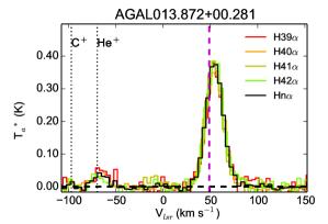
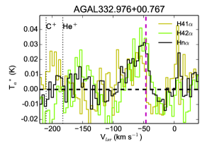
Figure 1: For two sources in our sample, each color represents an observed RRL H$n\alpha$ transition and the black line shows the stacked spectrum. The purple dashed lines indicate the systemic local standard of rest (lsr) velocity of the clump determined from the H¹³CO⁺(1$-$0) transition and the two vertical black dotted lines indicate expected positions of helium and carbon RRLs.

Table 2: Frequency, absorption oscillator strength, and detection rates of observed hydrogen millimeter recombination lines. The H$n\beta$, H$n\gamma$, and H$n\delta$ mm-RRLs are only detected toward clumps where the peak intensities of H$n\alpha$ mm-RRLs are brighter than 0.24, 0.62, and 0.54 Jy, respectively.

mm-RRL	Rest frequency	Absorption	Number of	Number of	Detection Rate
Transition	(MHz)	oscillator strength∗	Observed sources	Detected sources
H$n\alpha$	$--$	$-$	976	178	18 $\pm$ 1
H39$\alpha$	$106737.4$	7.725489	385	58	15 $\pm$ 2
H40$\alpha$	$99023.0$	7.916287	366	57	16 $\pm$ 2
H41$\alpha$	$92034.4$	8.107084	972	146	15 $\pm$ 1
H42$\alpha$	$85688.4$	8.297880	972	136	14 $\pm$ 1
H$n\beta$	$--$	$-$	976	65	7 $\pm$ 1
H48$\beta$	$111885.1$	1.342709	366	20	5 $\pm$ 1
H49$\beta$	$105301.9$	1.369046	385	26	7 $\pm$ 1
H50$\beta$	$99225.2$	1.395383	366	28	8 $\pm$ 1
H51$\beta$	$93607.3$	1.421720	366	28	8 $\pm$ 1
H52$\beta$	$88405.7$	1.448056	971	47	5 $\pm$ 1
H$n\gamma$	$--$	$-$	389	23	6 $\pm$ 1
H55$\gamma$	$109536.0$	0.482179	366	17	5 $\pm$ 1
H56$\gamma$	$103914.8$	0.490287	385	17	4 $\pm$ 1
H57$\gamma$	$98671.9$	0.498395	366	18	5 $\pm$ 1
H58$\gamma$	$93775.9$	0.506503	366	19	5 $\pm$ 1
H60$\gamma$	$84914.4$	0.522718	385	15	4 $\pm$ 1
H$n\delta$	$--$	$-$	389	22	6 $\pm$ 1
H60$\delta$	$110600.7$	0.230388	366	9	2 $\pm$ 1
H61$\delta$	$105410.2$	0.233881	385	9	2 $\pm$ 1
H62$\delta$	$100539.6$	0.237374	385	11	3 $\pm$ 1
H63$\delta$	$95964.6$	0.240867	366	10	3 $\pm$ 1
H64$\delta$	$91663.1$	0.244359	384	11	3 $\pm$ 1
H65$\delta$	$87615.0$	0.247852	383	7	2 $\pm$ 1

(*) Goldwire (1968); Menzel (1969).

2.3 Data reduction

The data reduction was performed using the CLASS program of the GILDAS package. Since the RRLs with the adjacent principal quantum numbers ($n$) and the same $\Delta n$ have similar energy levels and absorption oscillator strengths, resulting in similar intensities, it is possible to stack the spectra to improve the S/N of the emission. This technique has been successfully used in cm-RRLs surveys (e.g., Alves et al. 2010; Anderson et al. 2011). We show two examples of the stacked spectra in Fig. 1; the upper panel shows the four H$n\alpha$ transitions ($n$ = 39, 40, 41, and 42) of AGAL013.872$+$00.281, while the lower panel shows the H$n\alpha$ transitions ($n$ = 41 and 42) emission detect toward AGAL332.976+00.767. In both panels we show the profile of the combined stacked spectra (black line). The emission seen toward AGAL013.872$+$00.281 is clearly detected; however, the emission toward AGAL332.976+00.767 is ambiguous in the individual transitions but is detected at a significant level in the stacked line ($>3\sigma$). After stacking all transitions, a polynomial baseline of order 1 to 3 fitted to a 200 km s^-1 wide line-free velocity range was subtracted from the spectra.

In addition to the mm-RRLs, we also used the high number density and high column density tracing H¹³CO⁺(1$-$0) ($\nu$ = 86754.330 MHz) and N₂H⁺ (1$-$0) ($\nu$ = 93173.772 MHz) transitions to determine the systemic radial velocities of the associated dense molecular clumps. The velocities of the peak emission in the H¹³CO⁺(1$-$0) and N₂H⁺ (1$-$0) line spectra were determined using CLASS and are indicated in Fig. 1 by the vertical purple dashed line.

3 Results

3.1 Detection rates

Fitting Gaussian profiles to spectra of the stacked and individual transitions provided line parameters and rms levels. We used a peak intensity greater than 3 $\sigma$ as a threshold for detections. In total, we detected H$n\alpha$ emission toward 178 clumps and H$n\beta$, H$n\gamma$, and H$n\delta$ RRLs toward 65, 23, and 22 clumps, which represent 18%, 7%, 6%, and 6% of the full sample, respectively. Figure 2 shows one object in the sample where mm-RRL emission is detected in H$n\alpha$, H$n\beta$, H$n\gamma$, and H$n\delta$ transitions. The numbers of observed and detected sources, and detection rates of stacked lines (H$n\alpha$, H$n\beta$, H$n\gamma$, and H$n\delta$) and individual transition lines are summarized in Table 2. Variations in the numbers of observed sources in the individual transition lines occur because the IRAM 30m observation did not cover all transitions toward all clumps targeted. Clumps with detected mm-RRL are listed in Table 3 which also provides flags to indicate their association with mid-IR and radio continuum emission (these associations are discussed in more detail in a later section).

In general, the relative intensity of RRL emission changes with $\Delta n$ of the RRL. The intensities of small $\Delta n$ RRLs (i.e., H$n\alpha$ transition) are higher than the intensities of larger $\Delta n$ RRLs (i.e., H$n\beta$, H$n\gamma$, and H$n\delta$ transitions) (Towle et al. 1996). This explains the lower detection rates of $\Delta n>$ 1 RRLs for a given sensitivity. Furthermore, the H$n\alpha$ transition can be stimulated more easily by maser emission than higher-order transitions under non-LTE conditions, which can lead to an increase in their intensity and detection rate. In Sect. 3.2.1, we discuss whether the H$n\alpha$ mm-RRLs depart from LTE.

Table 3: Clumps detected with mm-RRLs.

ID	ATLASGAL	RA	Dec.	Dist	Log($M_{\rm clump}$)	Log($L_{\rm bol}$)	H$n\alpha$ vlsr	Systemic vlsr	WISE	Radio	Comments
No.	clump name	$\alpha$(J2000)	$\delta$(J2000)	(kpc)	(M⊙)	(L⊙)	(km s-1)	(km s-1)	mid-IR	emission
1	AGAL008.671$-$00.356	18:06:19.0	$-$21:37:28	$--$	$-$	$-$	$+$44	$+$35	IR-bright	Y	EGO
2	AGAL010.151$-$00.344	18:09:21.2	$-$20:19:28	$1.6$	2.11	$-$	$+$20	$+$9	Complex	Y
3	AGAL010.168$-$00.362	18:09:26.7	$-$20:19:03	$3.6$	3.01	$-$	$+$10	$+$14	Complex	Y	W31
4	AGAL010.323$-$00.161	18:09:01.4	$-$20:05:12	$3.5$	3.60	4.62	$+$5	$+$12	IR-bright	Y
5	AGAL010.472$+$00.027	18:08:37.9	$-$19:51:48	$8.6$	4.55	5.34	$+$60	$+$67	IR-bright	Y
6	AGAL010.624$-$00.384	18:10:28.6	$-$19:55:46	$4.9$	4.20	5.61	$+$0	$-$3	IR-bright	Y	W31
7	AGAL010.957$+$00.022	18:09:39.2	$-$19:26:28	$13.7$	4.15	5.10	$+$18	$+$21	IR-bright	Y
8	AGAL011.034$+$00.061	18:09:39.7	$-$19:21:20	$14.4$	3.84	5.02	$+$9	$+$15	IR-bright	Y
9	AGAL011.936$-$00.616	18:14:00.8	$-$18:53:24	$4.0$	3.61	4.97	$+$42	$+$38	IR-bright	Y
10	AGAL012.208$-$00.102	18:12:39.6	$-$18:24:14	$13.6$	4.58	$-$	$+$28	$+$24	IR-bright	Y
11	AGAL012.804$-$00.199	18:14:13.5	$-$17:55:32	$2.4$	4.03	5.11	$+$36	$+$36	IR-bright	Y	W33
12	AGAL013.209$-$00.144	18:14:49.3	$-$17:32:46	$4.6$	3.55	$-$	$+$50	$+$52	IR-bright	Y
13	AGAL013.384$+$00.064	18:14:24.9	$-$17:17:39	$1.9$	2.02	$-$	$+$14	$+$14	IR-bright	Y
14	AGAL013.872$+$00.281	18:14:35.6	$-$16:45:39	$4.4$	3.50	$-$	$+$52	$+$49	IR-bright	Y
15	AGAL015.013$-$00.671	18:20:21.3	$-$16:12:42	$2.0$	3.84	4.13	$+$8	$+$18	Complex	C	M17
16	AGAL015.024$-$00.654	18:20:17.9	$-$16:11:30	$2.0$	2.73	$-$	$+$20	$+$19	Complex	C	M17
17	AGAL015.029$-$00.669	18:20:22.4	$-$16:11:44	$2.0$	3.68	5.17	$+$10	$+$19	Complex	C	M17SW
18	AGAL015.051$-$00.642	18:20:18.7	$-$16:09:43	$2.0$	$-$	$-$	$+$21	$+$18	Complex	C	M17
19	AGAL015.056$-$00.624	18:20:15.4	$-$16:08:59	$2.0$	2.17	$-$	$+$22	$+$18	Complex	C	M17

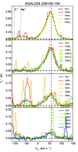
Figure 2: One of the mm-RRL spectra detected toward the ATLASGAL sources. Each color represents a different transition. The black lines are stacked mm-RRLs and the purple dashed lines indicate the velocity of the H¹³CO⁺(1$-$0) emission line. The vertical black dotted lines indicate positions of expected helium and carbon RRLs. Other emission lines are an unidentified molecular emission.

Table 4: Intensity and linewidth of mm-RRLs.

Stacked line	No. of sources	Speak (Jy)		linewidth (km s-1)
Transition		Mean (rms)	Median (rms)	Mean	$\sigma$	Standard error
H$n\alpha$	178	1.75 (0.14)	0.91 (0.15)	28.4	7.0	0.52
H$n\beta$	65	1.02 (0.14)	0.70 (0.06)	28.3	7.4	0.92
H$n\gamma$	23	0.37 (0.04)	0.29 (0.04)	28.5	7.5	1.57
H$n\delta$	22	0.25 (0.04)	0.18 (0.04)	27.2	8.4	1.80

Figure 3: Plot of Eq. (4.9) from Brocklehurst & Seaton (1972) with different electron densities ($n_{e}$). The gray area indicates observed mm-RRLs transitions (39 $\leq n\leq$ 65) in this paper. The curves show how the relationship between the linewidth ratio and the principal quantum numbers varies as a function of the electron density. The values $\Delta$v_P and $\Delta$v_D indicate the linewidths produced by pressure broadening and doppler broadening effects, respectively.

3.2 General properties of the mm-RRLs

In Table 4 we present a summary of the mean intensities and linewidths of the various stacked mm-RRL spectra. The mean and median peak intensities clearly decrease toward higher-order transitions while the mean linewidths for all transitions are similar (linewidth $\sim$30 km s^-1). Figure 3 shows how pressure broadening affects the observed linewidths as a function of the principal quantum number ($n$) and electron density. Even though there is a variation in the pressure broadening in the range of our observed transitions (gray filled area) for high electron densities ($\geq$ 10⁵ cm^-3), the pressure broadening of mm-RRLs from UC Hiis with typical density of 10⁴ cm^-3 (Kurtz 2005) is very small and can be neglected. The linewidths of mm-RRLs for all transitions considered here are, therefore, likely to be dominated by unresolved turbulent and thermal motions of the ionized gas. In addition, the linewidth ratio of higher-order to H$n\alpha$ transitions shows whether there is any pressure broadening affecting the mm-RRL (Viner et al. 1979): Mean linewidth ratios of H$n\beta$/H$n\alpha$, H$n\gamma$/H$n\alpha$, and H$n\delta$/H$n\alpha$ are 0.96$\pm$0.12, 0.93$\pm$0.10, and 0.89$\pm$0.15, respectively. Since the pressure broadening effect increases with principal quantum number ($n$) we expect to find significant variations from unity if there is significant pressure broadening in the gas; however, this is not seen suggesting that this effect is negligible. The relation of peak intensities and the linewidths of the H$n\alpha$ mm-RRLs is shown in Fig. 4. In general, evolved Hii regions such as UC Hii and compact Hii regions have been found to have linewidths of $\sim$30 km s^-1; however, broader RRL have been reported toward HC Hiis (linewidth $\geq$ 40 km s^-1; e.g., Sewilo et al. 2004). In Fig. 4, the linewidths of the majority of mm-RRLs are narrower than 40 km s^-1, which is consistent with the RRLs being associated with UC Hii regions. However, this plot also reveals nine clumps that have broader mm-RRL linewidths ($>$ 40 km s^-1), six of which have a S/N $>$ 5 and so are considered to be reliable. Such broad linewidths are normally found toward more compact Hii regions making these six sources potential HC Hii region candidates (source ID: N32, N49, N51, N62, N73, and N107 in Table 3) and we investigate some of these in more detail in Sect. 4.4.

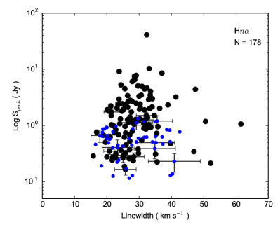
Figure 4: Distribution of H$n\alpha$ RRLs peak intensity as a function of linewidth. The blue dots indicate sources with mm-RRLs detected below 5 $\sigma$. The error bars are plotted for every 7th source chosen at random to show their range.

3.2.1 Excitation conditions

Comparing peak intensity ratios of H$n\alpha$ and higher-order RRLs is useful in order to diagnose whether the mm-RRLs are emitted under local thermodynamic equilibrium (LTE) or non-LTE conditions. Table 5 gives the measured mean ratios from the mm-RRLs and the expected ratios assuming LTE condition of pairs of transitions. In non-LTE conditions the measured ratio is lower than expected under LTE conditions, due to an increase in the H$n\alpha$ intensity from stimulated maser amplification than the higher-order lines, as seen in MWC349A (Thum et al. 1995).

The peak intensity ratios for the observed mm-RRLs are, on average, consistent with the corresponding LTE ratios within the 1 $\sigma$ scatter of the observed values. However, we note that the mm-RRLs from AGAL034.258+00.154 (ID: N49) and AGAL043.166+00.011 (ID: N55) show significantly lower peak intensity ratios (e.g., H$n\beta$/H$n\alpha$ (0.236$\pm$0.008 and 0.252$\pm$0.007), H$n\gamma$/H$n\alpha$ (0.096$\pm$0.008 and 0.102$\pm$0.007) and H$n\delta$/H$n\alpha$ (0.055$\pm$0.005 and 0.064$\pm$0.005)). A geometrical effect in a spherical Hii region with variable electron temperature and density could produce these low ratios (Walmsley 1990).

Since these transitions are observed with similar spatial resolution, the geometrical effect is not important. The H$n\alpha$ RRLs of the two sources might be enhanced by weak maser amplification even though their ratios do not deviate from LTE to the same extent as the well-known case of MWC349A (see Thum et al. 1995; Martín-Pintado 2002). Therefore, these two Hii regions are candidates for new RRL maser sources and observations are underway to investigate these sources in more detail. The results of these observations will be reported in a future paper.

Table 5: Ratio of mm-RRL transitions. The (#) indicates the number of sources that are detected in both transitions. These mean values are average values of individually measured ratios of sources in which both lines are detected.

	Mean peak intensity ratio
Pairs (#)	Observed	Under LTE
H$n\beta$/H$n\alpha$ (65)	0.31 $\pm$ 0.07	0.27
H$n\gamma$/H$n\alpha$ (23)	0.14 $\pm$ 0.02	0.13
H$n\delta$/H$n\alpha$ (22)	0.10 $\pm$ 0.02	0.07

3.3 Systematic velocities of the clumps

We used the H¹³CO⁺(1$-$0) and N₂H⁺ (1$-$0) transitions as a tracer of the systematic velocity of the dense molecular clumps (Beuther & Sridharan 2007). The H¹³CO⁺(1$-$0) emission was detected toward 170 sources, and so the N₂H⁺ (1$-$0) transition was used to determined the velocities for the other eight sources. Both of these transitions were observed simultaneously with the mm-RRL transitions and are available from the IRAM and Mopra data sets.

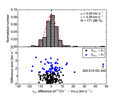
Figure 5: Upper panel: Histogram of the v_lsr difference between H¹³CO⁺(1$-$0) and H$n\alpha$ RRL. The bin size is 3.5 km s^-1. Lower panel: Distribution of peak velocity errors with respect to the v_lsr differences. The blue dots represent sources with weak mm-RRLs below 5 $\sigma$.

As seen in all of the examples given in Figs. 1 and 2, the peak velocity of the mm-RRL emission is similar to that of the thermal molecular transition, which indicates that the two emission features are likely to be associated with the same clump. Figure 5 shows the differences between H$n\alpha$ RRL and H¹³CO⁺(1$-$0) velocities. The velocity distribution is reasonably well fitted by a Gaussian profile (red dashed line) with a mean and standard error of 0.04 $\pm$ 0.35 km s^-1. This result is similar to that found in other cm- and mm-RRL studies made toward other samples of compact Hii regions (e.g., UC Hii; Churchwell et al. 2009) and GLIMPSE IRAC 8 $\mu$m bright Hii regions (Anderson et al. 2014). These studies found mean velocity differences in a range of $-$1.3 km s^-1 $\leq\Delta$ v${}_{lsr}\leq$ $+$1.5 km s^-1. The strong correlation between the velocities of the molecular and ionized gas supports the physical association between the two.

Although the correlation between the mm-RRL and H¹³CO⁺(1$-$0) velocities is generally very good, there are some sources where the velocity difference is larger than 15 km s^-1, which is more than three times the standard deviation ($\sigma$, 4.6 km s^-1). In particular, the mm-RRL velocity we measure for AGAL305.512+00.349 (ID: N82) is extremely offset with respect to the systematic velocity as marked in the bottom panel of Fig. 5. We note that in the majority of these cases the mm-RRL emission has a low S/N (see bottom panel of Fig. 5, blue dots) with the exception of AGAL301.136$-$00.226 (ID: N73), which is discussed in Sect. 4.4.

3.4 Relation between the molecular clouds and the Hii regions

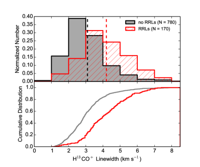
Figure 6: Distributions of H¹³CO⁺(1$-$0) linewidth for mm-RRLs associated (red) and mm-RRLs unassociated (gray) sources. Upper panel: Normalized histograms for the sources. The dashed lines represent mean values for each histogram. The bin size is 1.0 km s^-1. Lower panel: Cumulative distribution functions.

To investigate whether there is a dynamic link between the Hii regions and the associated molecular clumps, we compared the distribution of the mm-RRL and H¹³CO⁺(1$-$0) linewidths, and no correlation was found (the Spearman’s correlation coefficient, $\rho$, is 0.09). In Fig. 6, however, histograms and cumulative distributions of clumps with and without mm-RRL detection show a difference between the H¹³CO⁺(1$-$0) linewidths for the two different samples. The linewidths of H¹³CO⁺(1$-$0) toward clumps with mm-RRL detection (red curve) are notably broader than those toward clumps without a mm-RRL detection (gray curve), with mean linewidths of 4.18 $\pm$ 0.11 (red dashed line) and 3.08 $\pm$ 0.04 km s^-1 (black dashed line) for clumps with and without mm-RRL detection, respectively. A Kolmogorov-Smirnov (KS) test shows that the null hypothesis that the two samples are drawn from the same parent population is rejected with a $p-$value $\ll$ 0.001, implying that the existence of Hii regions traced by the mm-RRL detection contributes to the turbulence of the associated molecular clumps. This trend of molecular linewidth broadening with clump evolution is also confirmed by the results of Wienen et al. (2012) and Urquhart et al. (2013); both of these studies find a mean linewidth of the NH₃ transition (2.8 km s^-1) toward ATLASGAL clumps associated with radio continuum sources, which is significantly broader than that found toward clumps without an embedded mid-IR sources (a mean linewidth of 1.9 km s^-1).

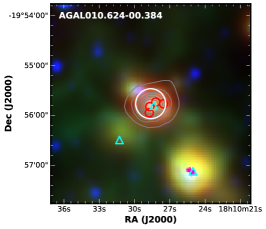
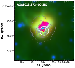
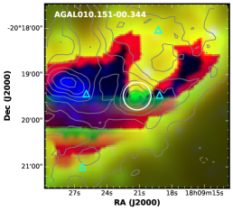
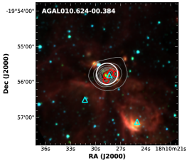
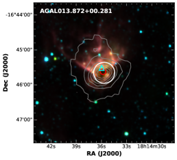
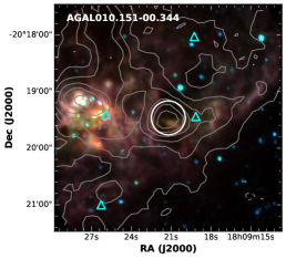
Figure 7: Clumps representative of the three typical mid-IR morphologies discussed in the text (from left to right: compact, extended, and complex.) Upper panel: WISE three-color composite images (4.6 (blue), 12 (green), and 22 $\mu$m (red)). Lower panel: GLIMPSE IRAC three-color composite images (3.6 (blue), 4.6 (green), and 8 $\mu$m (red)). Gray contour lines indicate 870 $\mu$m dust continuum emission from the ATLASGAL survey. The red circles and cyan triangles are 5 GHz CORNISH sources and 1.4 GHz NVSS sources. The white circles are centered on the pointing positions used for our Mopra and IRAM observations and their diameters approximate the FWHM beams size of these telescopes in the 85–100 GHz range. The ATLASGAL beam has a size of $19^{\prime\prime}$ FWHM.

3.5 Radio continuum and mid-IR counterparts

To further investigate the origin of the mm-RRLs, we examined mid-IR images and searched for embedded radio continuum sources coincident with the clumps. For example, because of its compactness a HC Hii region only emits weak radio emission that is optically thick throughout the radio range (i.e., $\nu$ $<$ 50 GHz where its flux density varies as $\nu^{2}$). Given this weak emission, they might not have been detected in past shallow radio surveys that were conducted at longer cm wavelengths.

We extracted mid-IR maps from the WISE and GLIMPSE surveys and created three-color images centered on the observed position. The mid-IR three-color images of three sources that are representative of compact, extended, and complex mid-IR emission are presented in Fig. 7. These images provides a useful way to identify embedded protostellar objects and to investigate their local environments. We searched WISE point source catalogs (Cutri et al. 2012) and identified mid-IR counterparts within a radius of 18″ (approximately the size of the ATLASGAL telescope beam) for 118 clumps. However, visual inspection of the three-color images reveals that many of the maps are affected by saturation indicating the presence of very bright sources within them. In total, we find mid-IR emission toward 127 clumps (including some sources that are saturated and that are not included in the WISE catalogs). We also find that the saturation in the maps toward 43 sources is so bad that they cannot be used to evaluate the distribution of the mid-IR emission; many of these are found toward well known star-forming regions such as M17 and G305 (Povich et al. 2007 and Hindson et al. 2012, respectively). We find no significant mid-IR emission associated with eight clumps.

We also utilized several large continuum surveys at wavelengths of 3, 6, and 20 cm (Zoonematkermani et al. 1990; Becker et al. 1994; Condon et al. 1998; Walsh et al. 1998; Giveon et al. 2005; White et al. 2005; Helfand et al. 2006; Urquhart et al. 2007, 2009; Purcell et al. 2013) to identify embedded compact and UC Hii regions. Using the same radius (18^′′) used to search for WISE counterparts, we identified 116 compact radio sources that are positionally coincident with clumps associated with mm-RRLs.

There is a possibility that radio sources other than Hii regions are the origin of the radio continuum, in particular extragalactic sources. The radio sources considered here are associated with the peak of the dust emission and are often extended, which is very unlikely for extragalactic sources. In addition, the extragalactic source counts are much lower at 5 GHz than at 1-2 GHz and hence the number of extragalactic sources, and the possibility of chance alignments with dust, is very low (Urquhart et al. 2013). Hii regions, even smaller UC Hiis, clearly show counterparts in mid-IR data (e.g., GLIMPSE data), whereas extragalactic sources are not normally associated with any mid-IR emission (Hoare et al. 2012; Purcell et al. 2013; Urquhart et al. 2013). Since all of the matched radio sources have an association with mid-IR emission, they can be classified as Hii regions.

In addition to the above-mentioned radio continuum surveys, 13 more clumps with mm-RRL detection have a 18 GHz radio counterpart in the AT20G survey (Ricci et al. 2004). In spite of the poor resolution and positional accuracy of the AT20G survey, these sources are associated with the clumps and mm-RRLs and so are likely to be Hii regions. Radio counterparts for five other clumps are also found in the literature (Kuchar & Clark 1997; Hindson et al. 2012, 2013). In total, compact radio emission is found to be associated with $\sim$75% of the whole mm-RRL associated sample. The positions of these radio sources are indicated in the images presented in Fig. 7. All of the radio sources are associated with clumps that are also associated with mid-IR emission, although ten of these are badly saturated in WISE 12 and 22 $\mu$m maps, but are recognizable in the GLIMPSE IRAC maps without any saturation. The positional correlation of the mid-IR source, the radio continuum emission, and the detection of the mm-RRL emission in 134 cases is consistent with the hypothesis that the ATLASGAL clumps are harboring compact Hii regions.

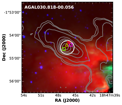
Figure 8: Potential HC Hii region candidate W43-MM1. It is one of the bright dust continuum peak of the W43 “mini-starburst” region (Sridharan et al. 2014). Mid-IR three-color composite images (GLIMPSE IRAC 3.6 $\mu$m (blue), 8 $\mu$m (green), and WISE 22 $\mu$m (red)). The gray contours trace the 870 $\mu$m dust continuum emission. The white circles are centered on the pointing position used for IRAM observation. The red star symbol indicates a WISE 22 $\mu$m point source. The yellow triangle is an OH maser (Szymczak & Gérard 2004). The green and purple squares indicate Class I and II CH₃OH masers (Larionov & Val’tts 2007; Szymczak et al. 2012).

We are left with 44 clumps toward which mm-RRL emission is detected, but which are not associated with a compact radio source. There are three possible explanations for these sources: 1) the mm-RRL emission is coming from a nearby evolved Hii region, 2) the mm-RRL is associated with an optically thick Hii region at cm wavelengths whose flux density is below the limits of the exiting cm-wavelength surveys, or 3) the clump has not been included in any high-resolution radio continuum surveys.

Almost certainly, the 127 clumps with a compact mid-IR source are undergoing star formation. Conversely, the absence of a potential embedded source suggests that the mm-RRL emission is likely to be associated with nearby Hii regions. In addition, we have already found large differences between the velocity of mm-RRL and the systemic velocity of the molecular gas for a number of associations which might be due to such contamination (Sect. 3.3). As previously mentioned, no mid-IR emission is detected toward eight of these clumps, one of which (N82) has a significant difference between the velocity of the mm-RRL and the systemic velocity of the clump, as have been marked in Fig. 5, and it is therefore likely that this association is due to contamination. We note that 3 of the 134 compact radio sources (N59, N73, N104) are matched to mm-RRL emission where the velocities of the mm-RRLs with respect to the molecular gas are larger than 15 km s^-1. Therefore, they are likely unassociated with molecular clumps and the result of contamination from nearby Hii regions. Nevertheless, they also have compact radio and mid-IR sources. It means that we cannot fully exclude the possibility that the large velocity difference is caused by other reasons such as internal turbulent motions of the Hii regions.

Owing to the relatively large size of the Mopra and IRAM beams, it is possible that some of the mm-RRL detections originate from large-scale Hii regions in close proximity to a significant number of clumps and not the star-forming regions associated with the ATLASGAL clumps. Bright and extended Hii regions might even be picked up by the sidelobes of the telescopes.

The radio counterparts found for the northern hemisphere clumps are drawn primarily from the CORNISH survey which is an unbiased 5 GHz radio continuum survey (Hoare et al. 2012), and so the third possibility that a particular clump has not been included in any high-resolution radio continuum surveys can be discarded. In this region of the plane we find 11 mm-RRL detections not associated with a compact radio source. Of these, nine are located near the intense star-forming regions M17, G34, W49, and W51. Their mid-IR images are almost completely saturated in the WISE 22 $\mu$m band and show complex GLIMPSE IRAC 8 $\mu$m emission. The non-detection of any compact radio continuum and the close proximity to star-forming complexes lead us to conclude that the mm-RRL emission is due to contamination and is not associated with the clumps. The remaining two sources, AGAL029.911$-$00.042 (ID: N30) and AGAL030.818$-$00.056 (ID: N37; see also Fig. 8), are associated with compact mid-IR emission. Source N30 is related to SiO molecular emission with high-velocity line wings, which indicates the presence of outflows from deeply embedded MYSOs (Csengeri et al. 2016). Source N37 is associated with masers (e.g., Class I & II methanol and OH masers) that also indicate an earlier stage than an evolved Hii region. Therefore, these two sources are good potential HC Hii region candidates.

The radio associations identified for clumps located in the southern hemisphere have largely been drawn from targeted observations of an MSX color selected sample of MYSOs (Urquhart et al. 2007) and methanol masers (Walsh et al. 1997). A consequence of this is that not all mm-RRL emitting clumps have been observed. Therefore, the detection of a mm-RRL may be revealing the location of Hii regions that have not previously been discovered at radio wavelengths. There are 25 mm-RRL sources detected in the fourth Quadrant that have not previously discussed; 19 are located near the edges of large complexes where mm-RRL emission is likely to be the result of contamination from evolved Hii regions; however, the remaining 6 detections are all associated with compact mid-IR emission and are likely to be good Hii region candidates.

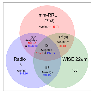
Figure 9: Venn diagram illustrating the distributions of ATLASGAL clumps (black numbers) that are in association with mm-RRL detection, radio continuum sources (only considering large continuum surveys for clumps without mm-RRL detection, while the number of radio sources with mm-RRL is based on complete, individual searches), and WISE 22 $\mu$m emission (only considering association with WISE 22 $\mu$m point sources). In addition, average integrated fluxes of total H$n\alpha$ and 6 cm radio continuum are given as red and blue numbers in Jy km s^-1 and mJy, respectively. The star (^∗) indicates that these 33 sources are saturated in WISE 22 $\mu$m emission and the dagger (^†) indicates that contaminated sources have been included. The numbers in parentheses represent 8 mid-IR dark sources among the 27 clumps with only mm-RRL and 8 potential Hii candidates among the 17 clumps with both the mm-RRL and the WISE 22 $\mu$m point source.

Figure 9 visualizes in a Venn diagram the association of the mm-RRL detected clumps with radio and infrared WISE 22 $\mu$m emission. It also provides average values of integrated 6 cm continuum (blue text) and mm-RRL (red text) intensities. In summary, we identify 44 sources that show mm-RRLs and are not matched to a compact radio source. Of these, 28 are located near some of the most intense star-forming regions in the Galaxy where the nature of the emission cannot be reliably determined. In addition, eight clumps are found to be mid-IR dark and therefore unlikely to harbor Hii regions; in all of these cases there is evidence of a nearby Hii region that is likely to be the source of the observed mm-RRL emission. Nevertheless, the fact that a mid-IR dark clump may contain an Hii region cannot be completely excluded in order to explain the mm-RRL detection toward the mid-IR dark clump. Finally, there are eight clumps that are associated with bright mid-IR emission, many of which are also associated with methanol masers; these are considered to be good Hii region candidates.

4 Analysis and discussion

4.1 Comparison of the mid-IR and radio properties

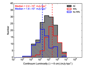
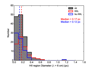
Figure 10: Upper panel: Radio continuum luminosity for sources with and without mm-RRL emission. The bin size is 0.5 dex. Lower panel: Hii region diameters. The bin size is 0.1 pc. The blue and red dashed lines indicate median values of the radio continuum luminosity and Hii region diameter for mm-RRL and non mm-RRL sources. The gray histograms of both plots show the distributions of the full sample

.

In the previous section we discussed the radio and mid-IR counterparts that are associated with clumps with mm-RRL detection. We found that the vast majority of the mm-RRL emission sources are associated with strong mid-IR emission and compact radio emission sources and these are therefore associated with compact Hii regions. The full sample of 976 observed ATLASGAL clumps also includes clumps associated with radio and mid-IR emission but toward which no mm-RRL emission has been detected. In this section we compare the mid-IR and radio properties of the Hii region with and without detectable mm-RRL emission in an effort to understand the differences between the two samples.

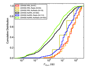
Figure 11: Cumulative flux distributions of WISE 22 $\mu$m point sources. The colors indicate associations with a detection of a mm-RRL and a radio continuum counterpart. WISE 22 $\mu$m point sources with fluxes over 330 Jy are excluded as the detectors saturate and the fluxes are unreliable.

Compact radio sources have been matched to 242 clumps (only considering the main large radio continuum surveys that we used when searching for radio counterparts) from the whole sample of 976 clumps ($\sim$25% of the sample), but mm-RRL emission is only detected toward slightly less than half of these. In Fig. 10 we compare the 6 cm continuum luminosity and Hii region diameter of radio sources with and without mm-RRL emission association. The information regarding radio sources, parental clumps, and heliocentric distances is provided in Table 6.

It is clear from the upper panel of Fig. 10 that the radio sources associated with mm-RRL emission are significantly brighter than those without. Such a clear difference is not found for the Hii region diameters, which are similar for both source groups. This suggests that the mm-RRL detectability is mainly sensitive to the radio continuum brightness of the Hii regions. We note that we only use the 6 cm continuum detections for the analysis presented here and the rest of the paper, as this data is available for the majority of the clumps and all of the surveys have a similar angular resolution and sensitivity leading to a consistent data set to study the continuum association.

Table 6: WISE 22 $\mu$m point sources and radio continuum sources matched with mm-RRLs detection.

		6 cm radio continuum			WISE 22 $\mu$m
No.		S${}_{\rm 6\,cm}$	$\int$S${}_{\rm 6\,cm}$	Angular diameter	$F_{\rm 22\,\mu m}$†	Distance
		(mJy/beam)	(mJy)	(″)	(Jy)	(kpc)
1		$667.5$	$795.0$	$3.6$	$12.3$	$--$
4		$13.8$	$170.3$	$19.0$	$--$	$3.5$
5		$34.6$	$57.7$	$2.2$	$--$	$8.6$
6		$360.6$	$2060.9$	$4.9$	$--$	$4.9$
7		$109.1$	$196.0$	$1.6$	$17.2$	$13.7$
8		$21.7$	$50.2$	$5.2$	$28.6$	$14.4$
9		$163.9$	$1155.9$	$5.7$	$186.9$	$4.0$
10		$72.2$	$207.9$	$2.4$	$4.2$	$13.6$
11		$287.9$	$12616.4$	$16.2$	$--$	$2.4$
12		$40.7$	$946.8$	$8.2$	$38.8$	$4.6$
13		$10.5$	$603.9$	$19.1$	$59.3$	$1.9$
14		$24.7$	$1447.6$	$15.4$	$--$	$4.4$
21		$97.7$	$519.3$	$3.1$	$40.9$	$17.1$
23		$48.0$	$1277.9$	$14.6$	$--$	$3.0$
24		$121.6$	$342.1$	$2.3$	$31.1$	$12.1$
25		$86.4$	$510.2$	$8.6$	$--$	$4.5$
27		$33.0$	$49.0$	$1.5$	$--$	$9.1$

6 cm radio continuum emission: Becker et al. (1994); White et al. (2005); Urquhart et al. (2007, 2009); Purcell et al. (2013). WISE 22 $\mu$m point source:  Cutri et al. (2012). Distance: Urquhart et al. (2014b); Csengeri et al. (2016).

Within a search radius of 18^′′ at a observed position, WISE 22 $\mu$m point sources are matched to 696 clumps in the sample ($\sim$70%) with 118 being associated with mm-RRL detections and 578 associated with mm-RRL quiet clumps. This would suggest that the majority of the sources observed are actively forming stars, with approximately 35% (242/696) of these already harboring young stellar objects and/or compact Hii regions. Fig. 11 shows the cumulative flux distributions of the WISE 22 $\mu$m counterparts for various associations with the mm-RRL detection and radio continuum counterpart. The WISE point sources without the bad flags are valid, but their fluxes brighter than 330 Jy are not reliable (see Csengeri et al. 2014 for more details). Therefore, the plots for fluxes of the WISE 22 $\mu$m counterparts have only used the WISE 22 $\mu$m point sources with a flux less than 330 Jy. It is clear that the mm-RRL samples (red and orange curves) are associated with the brightest WISE sources and the flux distributions are significantly different from WISE sources not associated with a mm-RRL (black curve). The distribution of the radio and mid-IR associated clumps (blue curve) is significantly different from both the radio quiet clumps and the radio loud and mm-RRL associated clumps (the KS test is able to reject the null hypothesis that these are drawn from the same parent population with a $p-$value $\ll$ 0.001).

We have previously shown that radio sources not associated with mm-RRL emission tend to have weaker continuum luminosities. The distribution of their mid-infrared fluxes shown in Fig. 11 reveals that they also tend to have significantly lower mid-IR emission. Both the radio and mid-IR emission are distance dependent quantities and it is therefore possible that these trends are due to a physical difference in the properties of the embedded objects or due to a distance bias. If these trends arise from physical differences in the embedded objects, we would expect to see separation between both radio source groups with mm-RRL and without, in radio and mid-IR flux distributions. To minimize the potential for bias we only use clumps associated with a single radio source in a searching radius; this ensures that the flux of the radio source is compared with a flux of the closest WISE point source and that the radio and mid-IR emission are related to the same ionizing star. The WISE 22 $\mu$m fluxes of 25 point sources matched with the radio sources are severely saturated. Therefore, we used the MSX 21 $\mu$m flux for those saturated sources instead of excluding them from the radio and mid-IR flux distributions. Fig. 12 shows a scatter plot of integrated 6 cm radio continuum flux as a function of the WISE 22 $\mu$m point source flux in association with mm-RRL detection. It is clear from this plot that the mm-RRLs are associated with the brightest radio sources and that this trend is largely independent of the mid-infrared emission. This is confirmed by a KS test ($p-$value $\ll$ 0.001). In other words, these two populations are likely to have different physical conditions and are not the result of a distance bias. In spite of the small $p-$value of the KS test, however, these two populations are not obviously separated in the distributions.

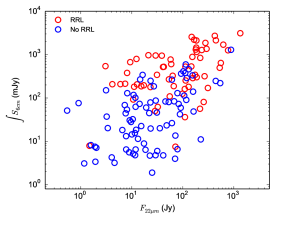
Figure 12: Integrated 6 cm radio continuum flux as a function of 22 $\mu$m flux for the mm-RRL quiet and bright radio sources.

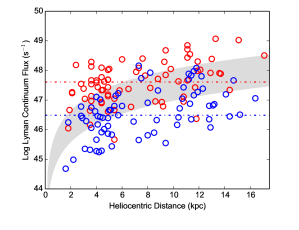
Figure 13: Lyman continuum flux as a function of heliocentric distance. The red and blue circles represent 6 cm radio continuum sources associated with and without mm-RRL sources. The gray area is filled between Lyman continuum fluxes estimated with median 6 cm integrated fluxes of radio sources associated with and without mm-RRL. The red and blue dot-dashed lines show median values in the Lyman continuum flux distributions for those sources, respectively.

Fig. 13 shows the Lyman continuum flux as a function of the heliocentric distance for radio continuum sources associated with ATLASGAL clumps. In this plot the mm-RRL associated and mm-RRL quiet radio sources are indicated as red and blue circles, respectively. The Lyman continuum fluxes are calculated using

$$\left(\frac{N_{i}}{\rm{photon\,s^{-1}}}\right)=9\times 10^{43}\,\,\left(\frac{\int S_{\nu}}{\rm{mJy}}\right)\,\,\left(\frac{D^{2}}{\rm{kpc}}\right)\,\,\left(\frac{\nu^{0.1}}{\rm{5\,GHz}}\right),$$ (1)

where $\int S_{\nu}$ is the integrated radio flux density measured at frequency $\nu$ and $D$ is the heliocentric distance to the source (Urquhart et al. 2013). This assumes the Hii regions are optically thin. This significantly underestimates the Lyman continuum flux for more compact Hii regions, but this assumption is justified (see next two sections). Radio continuum sources with mm-RRL mostly show Lyman continuum fluxes of $\geq 10^{47}$ photon s^-1, whereas the distribution of mm-RRL quiet radio sources tends to be associated with weaker Hii regions ($\sim 10^{46}$ photon s^-1). The median of the Lyman continuum flux distribution for radio sources with mm-RRL (red dot-dashed line) is close to $10^{48}$ photon s^-1, while the median of the Lyman continuum flux distribution for mm-RRL quiet radio sources (blue dot-dashed line) is less than $\sim 10^{46.5}$ photon s^-1.

The Lyman continuum fluxes of a large fraction of the radio sources with mm-RRL correspond well to the expected fluxes of late O-type stars. Hii regions ionized by O-type stars have Lyman continuum fluxes of $>10^{48}$ photon s^-1 and tend to have larger Hii region diameters than Hii regions associated with B-type stars that have fluxes $<10^{48}$ photon s^-1 (Urquhart et al. 2013). The sensitivity of the Mopra and IRAM observations appears to be limited to the detection of mm-RRL from the brightest late O-type stars.

4.2 The recombination line and radio continuum emission

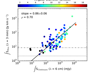
Figure 14: Integrated flux of radio continuum at 6 cm versus integrated flux of mm-RRLs at 3 mm. The black solid line indicates the best-fit line determined by a xy-bisector fit to the data. The black dot-dashed and dotted lines indicate 3 $\sigma$ integrated fluxes for IRAM 30m (2.22 Jy km s^-1) and Mopra 22m (8.54 Jy km s^-1). The color bar represents an angular diameter of continuum source in units of arc second. The black filled-circles show no angular size for unresolved radio sources. The errors on the integrated fluxes of mm-RRLs are 1.82 Jy km s^-1 on average.

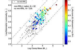
Figure 15: Bolometric luminosity as a function of clump mass for Hii regions presented in Urquhart et al. (2014b). The colors represent the mm-RRL luminosity. The gray dots indicate clumps without mm-RRL detection. The lower, middle and upper diagonal dot-dashed lines represent the $L_{\rm bol}/M_{\rm clump}$ = 1, 10, and 100 L${}_{\odot}/$M_⊙, respectively.

The radio continuum sources are smaller than the beam size of the Mopra and IRAM observations and so in some cases there are two or more radio sources located within the beam. It is thus likely that the observed mm-RRL emission has contributions from several radio continuum sources. To account for this we have summed the flux of all radio sources within the beam to obtain the total integrated radio flux. In Fig. 14 we plot spatially integrated 6 cm continuum flux density versus velocity-integrated mm-RRL flux. The mm-RRL detection thresholds are estimated from $\Delta w=\sigma\delta v\sqrt{N}$, where $\delta v$ is the channel width in units of km s^-1 and $N$ is the number of channels over which the emission is found (we have used a value of 10). Comparing the continuum and line fluxes we find them to be strongly correlated (the Spearman’s correlation coefficient, $\rho$, is 0.70 with a $p-$value $\ll$ 0.001). An xy-bisector fit to these data results in a slope of 0.86 $\pm$ 0.06.

Given that the mm-RRLs and radio continuum emission are tracing the same volume of gas, we would expect to find a linear relationship if the Hii regions continuum emission were optically thin. However, if it were optically thick at 6 cm we would expect the mm-RRL and continuum flux to deviate significantly from a linear relationship. The most compact Hii regions are the most likely to have optically thick emission (blue filled circles in Fig. 14); however, these regions do not deviate from the linear relationship. The fit to the fluxes shown in Fig. 14 is close to linear, which suggests that all of the Hii regions are broadly optically thin.

In Fig. 15 we show the relationship between the bolometric luminosity of all embedded Hii regions identified by the RMS survey (Lumsden et al. 2013) in each clump (Urquhart et al. 2014b) and the mass of the host clump. In this plot we also indicate the luminosity of the associated mm-RRL emission. When we calculated the luminosities of the mm-RRLs for the clumps with mm-RRL detections, we only used a subsample of the clumps with 6 cm radio continuum sources in order to reduce potential contamination by nearby Hii regions unassociated with the clumps, which is more of an issue for the lower resolution 20 cm NVSS survey.

There is a strong correlation between these three parameters with a clear trend for more luminous Hii regions giving rise to stronger mm-RRL emission and being associated with more massive clumps. We evaluated a Spearman’s correlation coefficient ($\rho$) for clumps with mm-RRL detection, without detection, and all clumps and obtained 0.67, 0.70, and 0.76 with $p-$values $\ll$ 0.0001, respectively. These results are higher than the partial Spearman’s correlation coefficient ($r=0.64$) of the MYSO, Hii region, and multiphase subsamples in Urquhart et al. (2014b).

The Spearman’s correlation coefficient ($\rho=0.67$) of the clumps with mm-RRL detection is significantly higher than the partial Spearman’s correlation coefficient ($r=0.53$) for the Hii region subsample which are CORNISH Hii regions of Urquhart et al. (2013). The clumps with mm-RRL detection are not only associated with mm-RRLs, but also have compact radio continuum sources. The clumps are therefore a subsample of the CORNISH Hii regions with a brighter flux than those of Urquhart et al. (2013). The fact that the mm-RRLs are associated with brighter radio continuum sources is also supported by the distribution seen in Fig. 12.

Clumps without a mm-RRL detection (gray dots) show a broad distribution from low to high masses and bolometric luminosities. On the contrary, clumps that are detected mm-RRLs (colored circles) tend to be associated with a large mass and bolometric luminosity. Similarly, the H¹³CO⁺(1$-$0) linewidths increase in clumps with the mm-RRL detection, as was shown in Sect. 3.4, although no clear correlation exists between the linewidth of H¹³CO⁺(1$-$0) and mm-RRLs for the mm-RRL luminosity in Fig. 15. It seems that the clumps with mm-RRL detection are more massive and have larger H¹³CO⁺(1$-$0) linewidths, the latter also implying that they are in virial equilibrium.

A possible reason for the lack of correlation between the linewidths of mm-RRL and H¹³CO⁺(1$-$0) may be that different size scales are involved; the linewidths of mm-RRL are linked to the small scales of the Hii regions, whereas the linewidths of H¹³CO⁺(1$-$0) are averages over the larger scale molecular clumps. However, we found by comparing samples with and without Hii regions that the Hii regions detected by mm-RRLs show enhanced turbulent motions in their environments, either directly or indirectly. This mm-RRL luminosity gradient and the H¹³CO⁺(1$-$0) linewidths reveal that the most massive clumps that host Hii regions and that are associated with strong mm-RRLs also have broader molecular linewidths.

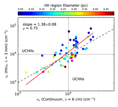
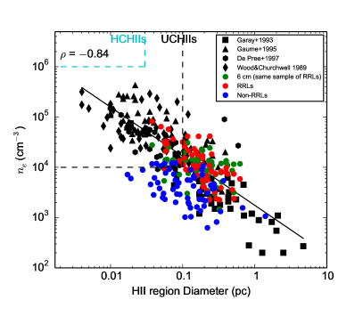
Figure 16: Left panel: $n_{e}$ derived from 6 cm radio continuum emission versus $n_{e}$ from mm-RRLs. Equality is indicated by the black dashed line. The dotted lines show the thresholds of electron density for UC Hii. The colors represent Hii region physical diameters in units of pc (see color bar) and the purple circles mark regions with diameter over 0.5 pc. The red line represents the best-fit line determined by an xy-bisector fit to the data.
Right panel: $n_{e}$ as a function of Hii region diameter. The red and green symbols show the distribution of the same sample of mm-RRL detections but where the election densities are derived from the the mm-RRL emission and 6 cm radio continuum emission, respectively. The black symbols indicate data from previous radio continuum surveys and the blue circles are radio sources toward which no mm-RRL emission is detected and where the electron density has been estimated from the of 6 cm radio continuum emission. The black solid line represents the best-fit line determined by a least-squares polynomial fit with one degree to the data of the previous radio continuum surveys (black symbols) and this mm-RRL surveys (red symbols).

4.3 Emission measure and electron density

In order to compare the physical parameters estimated by mm-RRL emission and 6 cm radio continuum, we need to calculate the emission measure (EM) of the continuum sources. The synthesized beam brightness temperature is calculated by Eq. 2 in Wood & Churchwell (1989)

$$T_{b}=\frac{S_{\nu}10^{-29}c^{2}}{2\nu^{2}k\Omega_{b}},$$ (2)

where $S_{\nu}$ is the peak flux density (mJy beam^-1), $\Omega_{b}$ is the solid angle of synthesized beam, $k_{\rm{b}}$ is the Boltzmann constant, $\nu$ is the rest frequency in Hz, and $c$ is the speed of light in m s^-1. The solid angle $\Omega_{b}$ is calculated from $\Omega_{b}=1.133\theta_{b}^{2}\,(sr)$, where $\theta_{b}$ is $1$$\aas@@fstack{\prime\prime}$$5$ for the CORNISH sources (Purcell et al. 2013), $2$$\aas@@fstack{\prime\prime}$$5$ for the RMS sources (Urquhart et al. 2007), and $4$$\aas@@fstack{\prime\prime}$$0$ for the sources identified by Becker et al. (1994). We assume $\tau_{C}\ll 1$ at 5 GHz and the Rayleigh-Jeans approximation, and thus $\tau_{C}$ = -ln$\left(1-T_{b}/T_{e}\right)$,

$${\rm EM}_{\rm cont}\,({\rm{cm}}^{-6}\,{\rm{pc}})=\frac{\tau_{C}}{8.235\times 10^{-2}a(\nu,T_{e})T_{e}^{-1.35}\nu^{-2.1}},$$ (3)

where $a$ is a correction factor of order unity (Mezger & Henderson 1967), which is 0.9938 at an electron density ($T_{e}$) of 10,000 K (Wood & Churchwell 1989) and $\nu$ = 5 GHz. Finally, in order to estimate an electron density ($n_{e}$), we use the physical diameters of the 6 cm radio continuum sources. If there are multiple continuum sources within the Mopra/IRAM beams, we estimate a new Hii region diameter from the combined area of radio continuum sources, i.e., $\Delta s$ = $\sqrt{\sum_{n=1}^{n}\Delta s_{n}^{2}}$. The $n_{e}$ is then given by

$$n_{e}=\sqrt{\frac{\rm EM}{\Delta s}}.$$ (4)

Since we confirmed that the linewidths of detected mm-RRLs are dominated by Doppler broadening (i.e., in LTE) (Sect. 3.2) and that the mm-RRLs seem to be optically thin (Sect. 4.2), we can determine the EM from the velocity-integrated intensity of the measured mm-RRL (Rohlfs & Wilson 2000). We estimate the EM using the following equation that takes account of the beam dilution effect,

$${\rm EM}_{\rm RRL}\,({\rm{cm}}^{-6}\,{\rm{pc}})=\frac{T_{e}^{3/2}}{576}\left(\frac{\theta_{\rm MB}^{2}+\theta_{s}^{2}}{\theta_{s}^{2}}\right)\left(\frac{\nu_{0}}{{\rm{GHz}}}\right)\left(\frac{\int T_{\rm MB}\,\Delta V}{K\,\mbox{km\,s${}^{-1}$}}\right),$$ (5)

where the beam filling factor, $f_{beam}$, is given by $\theta_{s}^{2}/(\theta_{\rm MB}^{2}+\theta_{s}^{2})$ in which $\theta_{s}$ is the angular diameter of the radio continuum source and $\theta_{\rm MB}$ is the antenna main-beam size. The angular diameter also presents a summed size for the physical diameters of radio continuum sources. Here we use the same $T_{e}$ as with the radio continuum data.

In the left panel of Fig. 16 we present a comparison of the $n_{e}$ calculated independently from the radio continuum and mm-RRL emission. There is a strong correlation between these two measurements with a correlation coefficient of $\rho=0.75$ with $p-$value $\ll 0.001$. The xy-bisector fit to these data gives a slope of 1.38 $\pm$ 0.08. There is a noticeable trend for the more compact radio sources to have higher $n_{e}$ in the measurement by the mm-RRL emission, which is expected since they are likely to be less optically thin.

In the right panel of Fig. 16 we show the relationship between $n_{e}$ and the Hii region diameter. The black symbols indicate the distribution of Hii regions reported in the literature, while the red and blue symbols show the properties of mm-RRL loud and quiet Hii regions discussed in this paper. There is clearly a strong correlation between these parameters ($\rho=-0.84$ with $p-$value $\ll 0.001$).

As previously discussed, we have found that the detected mm-RRLs tend to be associated with brighter Hii regions, many of which are driven by O-type stars. Fig. 16 reveals that the mm-RRLs tend to be associated with Hii regions that are more evolved than the UC Hii region stage. They also cover a similar range of physical scales to the mm-RRL quiet Hii regions, but have significantly higher $n_{e}$, which suggests that they are driven by more massive stars. Comparing these results to the typical $n_{e}$ and diameters of HC Hii (cyan dashed line; diameter $\leq$ 0.03 pc and $n_{e}$ $\geq$ 10⁵ cm^-3) and UC Hii (black dashed line; diameter $\leq$ 0.1 pc and $n_{e}$ $\geq$ 10⁴ cm^-3) (Kurtz et al. 2000), we find that most of the mm-RRL sources correspond to compact Hii regions with a few located in the UC Hii region part of the parameter space. We note that none is located in the HC Hiis parameter space; however, this plot only includes mm-RRL sources that have been matched with 6 cm radio continuum emission and so may be biased away from HC Hii regions as these tend to be optically thick at this frequency and are therefore less likely to be detected. As discussed in Sect. 3.5, we have identified a number of new Hii region candidates, and although the nature of these objects needs to be confirmed, this sample does include a few good potential HC Hii region candidates.

The results obtained from the mm-RRL parameters are consistent with the results determined from the radio continuum. This demonstrates the feasibility and complementarity of using mm-RRL observations to identify and parameterize compact Hii regions. Furthermore, mm-RRL observations have a couple of distinct advantages over conventional searches (e.g., radio continuum and mid-IR color selection) as all Hii regions should be optically thin at 3 mm and provide velocity information that can be used to derive distances and identify their natal molecular cloud.

4.4 Potential young Hii regions

For a while, high-mass stars during their early evolutionary phase as HC Hii regions still show activities such as accretion, infall, and outflow. As discussed in Sect. 4.3, although we have found that the properties of most sources are indicative of compact and UC Hii regions, we have identified three cases in which broad non-thermal motions mark potential young Hii regions.

In Sect. 3.2, we report broad mm-RRLs from nine clumps that have linewidths broader than 40 km s^-1. Roughly 30% of UC Hiis and 50% of HC Hiis are known to be associated with such broad RRLs observed at cm-wavelengths (Jaffe & Martín-Pintado 1999). Such broad RRL objects (BRLOs) are thought to be linked to a limited period having ionized outflows before the more evolved UC Hii phase (Jaffe & Martín-Pintado 1999; Sewilo et al. 2004; Sewiło et al. 2008; Keto et al. 2008; Zhang et al. 2014; Guzmán et al. 2014). Interestingly, one of the nine BRLOs, N73, has a velocity offset of its mm-RRL velocity with respect to its systemic velocity. This could be due to the influence of contamination by nearby Hii regions. Nevertheless, N73 is not only associated with a bright WISE 22 $\mu$m and unresolved radio continuum sources but is also coincident with an ionized outflow candidate reported by Guzmán et al. (2012). The ionized outflow candidate was explained to be an optically thick, expanding HC Hii (Purser et al. 2016). However, there is still no satisfactory explanation that is consistent with the origin of such BRLOs, although ionized outflows, disk winds, bow shocks, champagne flows, and inflows models (Jaffe & Martín-Pintado 1999) have been suggested to explain this phenomenon.

The second piece of evidence for the extreme youth of some Hii regions is the existence of stimulated (maser) emission in the mm-RRLs of N49 and N55. The mm-RRLs of these two clumps seem to be weakly enhanced by maser amplification. Radio recombination line maser emission is a very rare phenomenon and to date only two sources, WMC 349A and Mon R2 (Martin-Pintado et al. 1989; Jiménez-Serra et al. 2013), have been confirmed as RRL maser sources. According to these studies, the RRL maser phenomenon is linked to the structure and kinematics of the internal ionized gas rather than the nature of the source, and therefore the maser emission could be expected toward some young Hii regions showing high internal electron density that are modified by ionized stellar winds. Observing higher frequency, i.e., lower $n$ (sub)mm-RRLs, would also be helpful; such observations toward MWC 349A have revealed that the line shape becomes more and more asymmetric with decreasing $n$, developing a pronounced double-peaked shape (Thum et al. 1995; Martín-Pintado 2002; Jiménez-Serra et al. 2013). Interferometric observations are needed to confirm the RRL masers, similar to the confirmation of Mon R2 using high-resolution observations (Jiménez-Serra et al. 2013).

We have found mm-RRLs toward eight clumps without a radio counterpart. In particular, some of these (e.g., N37 as shown in Fig. 8) do not show extended 22 $\mu$m or 8 $\mu$m emission, but are associated with various masers such as OH, H₂O, Class I & II CH₃OH. Source N37, also known as W43-MM1, is considered to be a hot core and has multiple outflows (Motte et al. 2003; Sridharan et al. 2014). In addition, wing features seen in SiO emission, like the case of N30, (Csengeri et al. 2016) support the existence of outflows. Regardless of the absence of radio counterparts, the detections of the maser emission and the wings of SiO suggest that the detected mm-RRLs are produced from embedded young Hii regions in the clumps, but further mm- and submm-RRL observations at the high resolution and sensitivity provided by interferometers are necessary to study their properties in detail.

5 Summary and conclusions

We carried out 3 mm spectral line observations toward 976 dense clumps identified by the ATLASGAL survey ($-$60° $\leq\ell\leq+$60°). The sample was carefully selected to include a wide range of evolutionary stages from starless clumps to protostellar and compact Hii region stages. The observed spectra included a number of mm-RRLs and thermal molecular line transitions allowing a range of physical and environmental conditions to be investigated at the same angular resolution.

We have detected H$n\alpha$ mm-RRL emission toward 178 ATLASGAL clumps; H$n\beta$, H$n\gamma$, and H$n\delta$ transitions have been detected toward 65, 23, and 22 clumps, respectively. Inspecting mid-IR images and high-resolution radio continuum surveys, we are able to associate 134 of these mm-RRL detections with compact and UC Hii regions previously identified in the literature. This represents the largest mm-RRL sample so far reported and provides a new method of identifying and parameterizing Hii regions. Comparing the radio and mid-IR fluxes of the mm-RRL quiet and loud sources, we find that they are associated with the brightest continuum sources. Thus, because of the limited sensitivity of our observations we were not able to detect mm-RRLs toward an additional $\sim$126 Hii regions. Analysis of the ratios of the different mm-RRL transitions reveals that the lines are formed under LTE conditions.

Comparing the systemic velocity of the molecular material and the velocity of the ionized gas traced by the mm-RRL emission ($\sigma<$ 5 km s^-1) reveals a strong correlation between the two, which is consistent with the mm-RRL emitting Hii regions still being associated with their parental molecular clumps. We expected feedback from the embedded Hii regions to have a direct effect on the global turbulent motion in their molecular clumps. Comparing the H¹³CO⁺(1$-$0) linewidth of the mm-RRL associated and unassociated clumps, we find that the associated clumps tend to be more turbulent. However, we cannot reject the possibility that this is due to the Larson size-line width relation (Larson 1981).

We find a strong correlation between the integrated 6 cm radio continuum and mm-RRL emissions (the correlation coefficient $\rho=0.70$). This result implies that the 6 cm continuum and mm-RRL emissions are tracing the same ionized nebula. We also find that the Lyman continuum fluxes for these mm-RRL source are associated with evolved Hii regions driven by late O-type stars and the reason for large Hii region diameters ($\sim$0.5 pc) is that the Hii regions driven by O-type stars expand faster than B-type stars.

Of the remaining 44 mm-RRL detections that are not confirmed with radio counterparts, 36 are thought to be associated with nearby evolved Hii regions, while 8 detections are considered to be potential new Hii region candidates; these will need to be confirmed by future high-resolution and high-sensitivity radio continuum observations.

In this paper we have explored a new method of identifying compact Hii regions using mm-RRL emission. We have identified 142 genuine Hii regions (including the 8 potential Hii regions) and analysis of the line parameters has produced results that are consistent with those obtained from the radio continuum emission. We have therefore demonstrated that mm-RRLs are a viable and complementary method of identifying compact Hii regions and investigating their physical properties. Furthermore, mm-RRL observations have some inherent advantages over studies that merely analyze continuum emission in that they provide velocity information, which can be used to match the regions to their host clumps and to determine their Galactic locations.

Appendix A Comparison of cm- and mm-RRLs detected toward Hii regions

So far, RRL studies with single-dish telescopes and interferometers have mostly focused on RRLs at cm wavelength. There are only a few mm-RRL surveys that were conducted toward small samples biased toward a specific evolutionary phase such as UC Hii or HC Hii regions. Our new survey investigates for the first time the general properties of mm-RRLs toward a large sample and in this Appendix, we take a look at the overall properties of mm-RRLs in comparison with cm-RRLs of previous large surveys.

Table 7 is a summary of cm- and mm-RRL surveys used in this comparison. The RRLs surveys were carried out at different wavelengths with various beam sizes and targeted on different evolutionary phases of Hii regions, from UC Hii to extended Hii regions. The Hii regions of Caswell & Haynes (1987) and Lockman (1989) were classified by 6 cm radio continuum surveys with single-dish telescopes, which have a poor spatial resolution for identifying small Hii regions. These Hii regions could be in different evolutionary phases of Hii region. Therefore, in comparisons they are considered to be general Hii regions that are denoted by Hiis here. Fig. 17 shows the cumulative distributions of RRL linewidths, in which the Hiis (a black distribution) combines cm-RRLs from Lockman (1989) and Caswell & Haynes (1987).

Table 7: Hydrogen radio recombination line surveys.

Survey	H$n\alpha$ transition	$\lambda$	Beam size	No.
This paper	H39$\alpha$ $-$ H42$\alpha$	3 mm	29′′ $-$ 36′′	178
Churchwell+10	H30$\alpha$	1.3 mm	12′′	25
Lockman+89	H87$\alpha$ $-$ H88$\alpha$	3 cm	180′′	462
Anderson+11	H88$\alpha$ $-$ H93$\alpha$	4 cm	73′′ $-$ 89′′	603
Caswell+87	H109$\alpha$ $-$ H110$\alpha$	6 cm	264′′	317

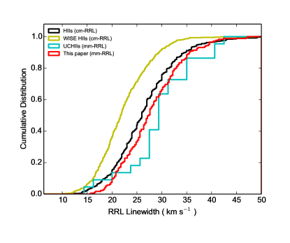
Figure 17: Cumulative distributions of RRL linewidths for this paper (red line) and previous surveys (yellow line: Anderson et al. 2011; black line: Lockman 1989; Caswell & Haynes 1987; and cyan line: Churchwell et al. 2010).

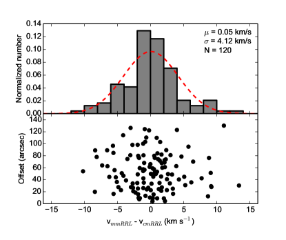
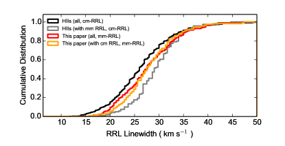
Figure 18: Upper panel: Velocity difference between mm-RRL and cm-RRL for sources where the beams of the surveys overlap (top plot). The velocity difference as a function of an offset between the mm-RRL and cm-RRL pointing centers (bottom plot). Lower panel: Cumulative distributions of cm- (gray) and mm-RRLs (orange) for clumps where the velocity difference between the cm- and mm-RRLs is within 15 km s^-1.

In Fig. 17, there is an obvious difference between linewidths of RRLs of the WISE selected Hiis (WISE Hiis) from Anderson et al. (2011) and the other samples. The linewidths of WISE Hiis are significantly narrower (mean width of 22.3 km s^-1) than the other surveys with mean values between 26.8 and 33.4 km s^-1. Kolmogorov-Smirnov tests are able to reject the null hypothesis, that the linewidths of the WISE Hii regions are similar to the other surveys, with very small $p-$values $\ll$ 0.001, implying differences in the properties of the Hii regions samples. In fact, the WISE Hiis, which are classified by 8 $\mu$m emission in GLIMPSE IRAC maps, include ionized bubbles, as well as more evolved Hii regions (Anderson et al. 2011). The sample (UC Hiis) of Churchwell et al. (2010) seems to be offset from the cm Hiis and from the sources discussed in this paper. However, the size of the sample is too small to be reliable and a null hypothesis that all of three samples are similar cannot be rejected because of a $p-$value (0.03) greater than 1%.

In Fig. 17, the cm-RRLs of Hiis and the mm-RRLs from this paper show similar linewidth distributions, although the cm-RRLs can be significantly affected by pressure broadening. The histogram in the upper panel of Fig. 18 shows velocity differences that are less than 15 km s^-1 toward the majority of sources (120 clumps) and therefore suggest that the cm- and mm-RRLs are tracing on common Hii regions. In the bottom plot of the upper panel the scatter dots show the distribution of offsets between observed positions of cm- and mm-RRLs as a function of the velocity difference. The scatter is homogeneous and further supports the idea that the cm- and mm-RRLs are emitted from the same region.

The cumulative distributions in the lower panel of the Fig. 18 show RRL linewidths of Hiis and this paper toward common Hii region which match in observed positions and velocities. In addition, the distribution for all sources are also displayed. The distribution of selected mm-RRLs from this paper (orange, with a mean linewidth of 28.5$\pm$0.5  km s^-1) does not change much compared to the total sample of mm-RRLs (red, mean linewidth of 28.4$\pm$0.5 km s^-1). However, the distribution of selected cm-RRLs from the Hiis sample (gray, mean linewidth of 29.6 $\pm$ 0.4 km s^-1) moves toward broader linewidths compared with the distribution of the whole Hiis sample (black, mean linewidth of 26.8 $\pm$ 0.3km s^-1). A KS test for the linewidths of the selected cm- and mm-RRLs samples also shows that a null hypothesis is invalid with a $p-$value $\ll$ 0.001. This suggests that the selected cm-RRLs are likely suffering from pressure broadening.

However, the cm-RRL surveys were carried out with 2 $\sim$ 6 times larger beams than ours. The broader cm-RRLs can also be affected by larger scale motions of the ionized gas in the larger beams. Our beams cover gas with a size of 1 pc at typical distance of 5 kpc. On the other hand, the beams of the cm-RRL surveys can capture gas with a size of about 4 $\sim$ 6 pc. Therefore, the linewidths of the cm-RRLs could also be a result of the blending of more than one Hii region leading to the observed broader linewidths.

References

- Alves et al. (2015) Alves, M. I. R., Calabretta, M., Davies, R. D., et al. 2015, MNRAS, 450, 2025
- Alves et al. (2010) Alves, M. I. R., Davies, R. D., Dickinson, C., et al. 2010, MNRAS, 405, 1654
- Anderson & Bania (2009) Anderson, L. D. & Bania, T. M. 2009, ApJ, 690, 706
- Anderson et al. (2014) Anderson, L. D., Bania, T. M., Balser, D. S., et al. 2014, ApJS, 212, 1
- Anderson et al. (2011) Anderson, L. D., Bania, T. M., Balser, D. S., & Rood, R. T. 2011, ApJS, 194, 32
- Becker et al. (1994) Becker, R. H., White, R. L., Helfand, D. J., & Zoonematkermani, S. 1994, ApJS, 91, 347
- Benjamin et al. (2003) Benjamin, R. A., Churchwell, E., Babler, B. L., et al. 2003, PASP, 115, 953
- Beuther & Sridharan (2007) Beuther, H. & Sridharan, T. K. 2007, ApJ, 668, 348
- Brocklehurst & Seaton (1972) Brocklehurst, M. & Seaton, M. J. 1972, MNRAS, 157, 179
- Carral et al. (1997) Carral, P., Kurtz, S. E., Rodríguez, L. F., De Pree, C., & Hofner, P. 1997, ApJ, 486, L103
- Caswell & Haynes (1987) Caswell, J. L. & Haynes, R. F. 1987, A&A, 171, 261
- Churchwell (1990) Churchwell, E. 1990, A&A Rev., 2, 79
- Churchwell (2002) Churchwell, E. 2002, ARA&A, 40, 27
- Churchwell et al. (2009) Churchwell, E., Babler, B. L., Meade, M. R., et al. 2009, PASP, 121, 213
- Churchwell et al. (2010) Churchwell, E., Sievers, A., & Thum, C. 2010, A&A, 513, A9
- Condon et al. (1998) Condon, J. J., Cotton, W. D., Greisen, E. W., et al. 1998, AJ, 115, 1693
- Contreras et al. (2013) Contreras, Y., Schuller, F., Urquhart, J. S., et al. 2013, A&A, 549, A45
- Csengeri et al. (2016) Csengeri, T., Leurini, S., Wyrowski, F., et al. 2016, A&A, 586, A149
- Csengeri et al. (2014) Csengeri, T., Urquhart, J. S., Schuller, F., et al. 2014, A&A, 565, A75
- Cutri et al. (2012) Cutri, R. M., Wright, E. L., Conrow, T., et al. 2012, Explanatory Supplement to the WISE All-Sky Data Release Products, Tech. rep.
- De Pree et al. (2004) De Pree, C. G., Wilner, D. J., Mercer, A. J., et al. 2004, ApJ, 600, 286
- Forster & Caswell (1989) Forster, J. R. & Caswell, J. L. 1989, A&A, 213, 339
- Gaume et al. (1995) Gaume, R. A., Claussen, M. J., de Pree, C. G., Goss, W. M., & Mehringer, D. M. 1995, ApJ, 449, 663
- Giannetti et al. (2014) Giannetti, A., Wyrowski, F., Brand, J., et al. 2014, A&A, 570, A65
- Giveon et al. (2005) Giveon, U., Becker, R. H., Helfand, D. J., & White, R. L. 2005, AJ, 130, 156
- Goldwire (1968) Goldwire, Jr., H. C. 1968, ApJS, 17, 445
- Gordon & Sorochenko (2002) Gordon, M. A. & Sorochenko, R. L., eds. 2002, Astrophysics and Space Science Library, Vol. 282, Radio Recombination Lines. Their Physics and Astronomical Applications
- Guzmán et al. (2012) Guzmán, A. E., Garay, G., Brooks, K. J., & Voronkov, M. A. 2012, ApJ, 753, 51
- Guzmán et al. (2014) Guzmán, A. E., Garay, G., Rodríguez, L. F., et al. 2014, ApJ, 796, 117
- Helfand et al. (2006) Helfand, D. J., Becker, R. H., White, R. L., Fallon, A., & Tuttle, S. 2006, AJ, 131, 2525
- Hindson et al. (2012) Hindson, L., Thompson, M. A., Urquhart, J. S., et al. 2012, MNRAS, 421, 3418
- Hindson et al. (2013) Hindson, L., Thompson, M. A., Urquhart, J. S., et al. 2013, MNRAS, 435, 2003
- Hoare et al. (2012) Hoare, M. G., Purcell, C. R., Churchwell, E. B., et al. 2012, PASP, 124, 939
- Hofner & Churchwell (1996) Hofner, P. & Churchwell, E. 1996, A&AS, 120, 283
- Jaffe & Martín-Pintado (1999) Jaffe, D. T. & Martín-Pintado, J. 1999, ApJ, 520, 162
- Jiménez-Serra et al. (2013) Jiménez-Serra, I., Báez-Rubio, A., Rivilla, V. M., et al. 2013, ApJ, 764, L4
- Keto & Klaassen (2008) Keto, E. & Klaassen, P. 2008, ApJ, 678, L109
- Keto et al. (2008) Keto, E., Zhang, Q., & Kurtz, S. 2008, ApJ, 672, 423
- Kuchar & Clark (1997) Kuchar, T. A. & Clark, F. O. 1997, ApJ, 488, 224
- Kurtz (2005) Kurtz, S. 2005, in IAU Symposium, Vol. 227, Massive Star Birth: A Crossroads of Astrophysics, ed. R. Cesaroni, M. Felli, E. Churchwell, & M. Walmsley, 111–119
- Kurtz et al. (2000) Kurtz, S., Cesaroni, R., Churchwell, E., Hofner, P., & Walmsley, C. M. 2000, Protostars and Planets IV, 299
- Kurtz et al. (1994) Kurtz, S., Churchwell, E., & Wood, D. O. S. 1994, ApJS, 91, 659
- Kurtz & Hofner (2005) Kurtz, S. & Hofner, P. 2005, AJ, 130, 711
- Ladd et al. (2005) Ladd, N., Purcell, C., Wong, T., & Robertson, S. 2005, PASA, 22, 62
- Larionov & Val’tts (2007) Larionov, G. M. & Val’tts, I. E. 2007, Astronomy Reports, 51, 756
- Larson (1981) Larson, R. B. 1981, MNRAS, 194, 809
- Lockman (1989) Lockman, F. J. 1989, ApJS, 71, 469
- Lumsden et al. (2013) Lumsden, S. L., Hoare, M. G., Urquhart, J. S., et al. 2013, ApJS, 208, 11
- Martín-Pintado (2002) Martín-Pintado, J. 2002, in IAU Symposium, Vol. 206, Cosmic Masers: From Proto-Stars to Black Holes, ed. V. Migenes & M. J. Reid, 226
- Martin-Pintado et al. (1989) Martin-Pintado, J., Bachiller, R., Thum, C., & Walmsley, M. 1989, A&A, 215, L13
- Menzel (1969) Menzel, D. H. 1969, ApJS, 18, 221
- Mezger & Henderson (1967) Mezger, P. G. & Henderson, A. P. 1967, ApJ, 147, 471
- Motte et al. (2003) Motte, F., Schilke, P., & Lis, D. C. 2003, ApJ, 582, 277
- Povich et al. (2007) Povich, M. S., Stone, J. M., Churchwell, E., et al. 2007, ApJ, 660, 346
- Price et al. (2001) Price, S. D., Egan, M. P., Carey, S. J., Mizuno, D. R., & Kuchar, T. A. 2001, AJ, 121, 2819
- Purcell et al. (2013) Purcell, C. R., Hoare, M. G., Cotton, W. D., et al. 2013, ApJS, 205, 1
- Purser et al. (2016) Purser, S. J. D., Lumsden, S. L., Hoare, M. G., et al. 2016, MNRAS, 460, 1039
- Ricci et al. (2004) Ricci, R., Sadler, E. M., Ekers, R. D., et al. 2004, MNRAS, 354, 305
- Rohlfs & Wilson (2000) Rohlfs, K. & Wilson, T. L. 2000, Tools of radio astronomy
- Schuller et al. (2009) Schuller, F., Menten, K. M., Contreras, Y., et al. 2009, A&A, 504, 415
- Sewilo et al. (2004) Sewilo, M., Churchwell, E., Kurtz, S., Goss, W. M., & Hofner, P. 2004, ApJ, 605, 285
- Sewiło et al. (2008) Sewiło, M., Churchwell, E., Kurtz, S., Goss, W. M., & Hofner, P. 2008, ApJ, 681, 350
- Shepherd & Churchwell (1996) Shepherd, D. S. & Churchwell, E. 1996, ApJ, 472, 225
- Sridharan et al. (2014) Sridharan, T. K., Rao, R., Qiu, K., et al. 2014, ApJ, 783, L31
- Szymczak & Gérard (2004) Szymczak, M. & Gérard, E. 2004, A&A, 414, 235
- Szymczak et al. (2012) Szymczak, M., Wolak, P., Bartkiewicz, A., & Borkowski, K. M. 2012, Astronomische Nachrichten, 333, 634
- Thum et al. (1995) Thum, C., Strelnitski, V. S., Martin-Pintado, J., Matthews, H. E., & Smith, H. A. 1995, A&A, 300, 843
- Towle et al. (1996) Towle, J. P., Feldman, P. A., & Watson, J. K. G. 1996, ApJS, 107, 747
- Urquhart et al. (2007) Urquhart, J. S., Busfield, A. L., Hoare, M. G., et al. 2007, A&A, 461, 11
- Urquhart et al. (2014a) Urquhart, J. S., Csengeri, T., Wyrowski, F., et al. 2014a, A&A, 568, A41
- Urquhart et al. (2009) Urquhart, J. S., Hoare, M. G., Purcell, C. R., et al. 2009, A&A, 501, 539
- Urquhart et al. (2014b) Urquhart, J. S., Moore, T. J. T., Csengeri, T., et al. 2014b, MNRAS, 443, 1555
- Urquhart et al. (2013) Urquhart, J. S., Thompson, M. A., Moore, T. J. T., et al. 2013, MNRAS, 435, 400
- Viner et al. (1979) Viner, M. R., Vallee, J. P., & Hughes, V. A. 1979, ApJS, 39, 405
- Walmsley (1990) Walmsley, C. M. 1990, A&AS, 82, 201
- Walsh et al. (1998) Walsh, A. J., Burton, M. G., Hyland, A. R., & Robinson, G. 1998, MNRAS, 301, 640
- Walsh et al. (1997) Walsh, A. J., Hyland, A. R., Robinson, G., & Burton, M. G. 1997, MNRAS, 291, 261
- Walsh et al. (2014) Walsh, A. J., Purcell, C. R., Longmore, S. N., et al. 2014, MNRAS, 442, 2240
- White et al. (2005) White, R. L., Becker, R. H., & Helfand, D. J. 2005, AJ, 130, 586
- Wienen et al. (2012) Wienen, M., Wyrowski, F., Schuller, F., et al. 2012, A&A, 544, A146
- Wood & Churchwell (1989) Wood, D. O. S. & Churchwell, E. 1989, ApJS, 69, 831
- Wright et al. (2010) Wright, E. L., Eisenhardt, P. R. M., Mainzer, A. K., et al. 2010, AJ, 140, 1868
- Wyrowski et al. (2008) Wyrowski, F., Brooks, K., Beuther, H., et al. 2008, Molecular fingerprints of an unbiased sample of Galactic massive star forming clumps, ATNF Proposal
- Wyrowski et al. (2009) Wyrowski, F., Brooks, K., Beuther, H., et al. 2009, Molecular fingerprints of an unbiased sample of Galactic massive star forming clumps II., ATNF Proposal
- Zhang et al. (2014) Zhang, C.-P., Wang, J.-J., Xu, J.-L., Wyrowski, F., & Menten, K. M. 2014, ApJ, 784, 107
- Zinnecker & Yorke (2007) Zinnecker, H. & Yorke, H. W. 2007, ARA&A, 45, 481
- Zoonematkermani et al. (1990) Zoonematkermani, S., Helfand, D. J., Becker, R. H., White, R. L., & Perley, R. A. 1990, ApJS, 74, 181