A study of periodograms standardized using training data sets and application to exoplanet detection

Abstract

When the noise affecting time series is colored with unknown statistics, a difficulty for sinusoid detection is to control the true significance level of the test outcome. This paper investigates the possibility of using training data sets of the noise to improve this control. Specifically, we analyze the performances of various detectors applied to periodograms standardized using training data sets. Emphasis is put on sparse detection in the Fourier domain and on the limitation posed by the necessarily finite size of the training sets available in practice. We study the resulting false alarm and detection rates and show that standardization leads in some cases to powerful constant false alarm rate tests. The study is both analytical and numerical. Although analytical results are derived in an asymptotic regime, numerical results show that theory accurately describes the tests’ behaviour for moderately large sample sizes. Throughout the paper, an application of the considered periodogram standardization is presented for exoplanet detection in radial velocity data.

I Introduction

I-A Considered problem and application

Detecting sinusoids in noise is one of the most studied problems in signal processing. Sinusoid detection is classically based on Fourier analysis, which benefits from a considerable set of statistical results. Often, the assumptions required for these results to hold are :
(i) Under the null hypothesis ($\mathcal{H}_{0}$ : noise only), the random process $X$ is stationary Gaussian with known statistics;
(ii) The time series $\{X(t_{j})\}_{j=1,\cdots,N}$ is regulary sampled, in which case Fourier analysis is performed through the periodogram [1, 2]

$$P(\nu):=\frac{1}{N\Delta t}\Big{|}\sum_{j=1}^{N}X(t_{j})\mathrm{e}^{-{\rm{i}}2\pi\nu j\Delta t}\Big{|}^{2},$$ (1)

where $\nu$ is the considered frequency, $N$ the number of samples and $\Delta t$ the time sampling step;
(iii) The number of samples $N$ is large (asymptotic regime);
(iv) The periodogram is evaluated at Fourier frequencies.
Assumptions (i)$-$(iv) allow to characterize the statistical properties of the periodogram as an estimate of the power spectral density (PSD)[3, 4, 2, 5, 6, 7, 8, 9]. In particular, any finite set of periodogram ordinates near some fixed frequency are asymptotically independent and exponentially distributed with parameters dependent on the noise PSD at the relevant frequencies (this assumption actually extends to linear processes other than Gaussian, see Th. 4 of [9]). In detection, such properties can be exploited to obtain the probabilities of false alarm and detection of tests based on periodogram ordinates.

Despite a large literature on the subject, the detection of periodic signals remains an active field of research because in practical situations some (or all) assumptions (i)-(iv) above may not be met. Before reviewing some such situations, it is worth introducing the application that motivated the present study (the proposed detection approach may cover other applications, however).

With almost $3\,000$ confirmed exoplanets and nearly $2\,500$ candidates (in September 2016, www.exoplanets.org), the detection of extrasolar planets is an extremely active research field in Astrophysics since two decades. This field benefits from constant technological improvements allowing extremely low noise detectors [10] and long (months to years) spaceborne observations with high (a few tens of seconds) sampling rates [11, 12, 13]. The Radial Velocity (RV) technique is one method for exoplanet detection. When planets orbit a host star, the resulting gravitational force creates a periodic displacement of the star. This induces a modulation of the RV of the star with respect to (w.r.t.) Earth, which translates into a periodic Doppler shift of the stellar light. The RV technique consists in detecting such variations in stellar RV time series [14, 15].
Modern instrumental performances have reached signal to noise ratios allowing, in principle, to detect exoplanets comparable to the Earth by the RV method. However, at such low levels of instrumental noise, a new critical and limiting issue appears. The stellar surface can be seen as a boiling fluid, with millions of convection cells generating upward and downward plasma flows visible under the form of granules having typical lifetime of a few minutes. These motions generate random fluctuations in the measured RV of the star that can mimic, or hide, exoplanetary signatures. The case of $\alpha$ Centauri Bb planet, a detection claimed in 2012 [16] (with an evaluated $P$-value of $0.02\%$) and since then subject to controversy [17, 18], is one example showing how our incomplete knowledge of the noise affects the reliability assigned to exoplanet detection claims. This specific issue motivated the present study.
A key point is that in parallel to technological advances, astrophysicists have continuously improved stellar models and elaborated numerical simulation codes able to account for the complex interplay of various astrophysical processes in the star’s interior and surface. Recent works demonstrate that granulation noise can be reproduced by large scale numerical simulations in a reliable way [19]. This suggests the possibility of using such simulations to calibrate the detection process, as RV time series are strongly affected by this stellar noise. The present study shows that one such calibration indeed leads to improved control of the statistical significance and to detection tests with increased power.

I-B Unknown noise statistics: related works

Turning back to the deviations encountered in practice w.r.t. assumptions (i)$-$(iv) above, this work will be primarily interested in the case of an incomplete knowledge of the noise statistics under the null hypothesis (i.e., relaxing condition (i); we mention in the last section perspectives to relax the other conditions). In this situation, the distribution of $P$ under the null is not known and consequently the significance level (the size) of the test is not known either. Constant false alarm rate (CFAR) detectors have been devised when the noise is white [20, 21, 22]. When the noise is colored, the detection problem is more complicated. In practice, two approaches can be followed. The first approach is simply to ignore possible noise correlations and to apply tests designed for white noise. However, as will be illustrated in this study, the statistical behavior of the resulting testing procedure may be hazardous, with unpredictable significance level and poor power (see also [23] on this point).
A more sophisticated approach consists of estimating the noise PSD (called $S_{E}$ below) so that condition (i) above is considered to hold approximately. This estimate can then be used to calibrate the periodogram of the data $P(\nu)$, leading to a frequency-wise standardized periodogram of the form

$$\widetilde{P}(\nu\;|\;\widehat{S}_{E}):=\frac{P(\nu)}{\widehat{S}_{E}(\nu)}.$$ (2)

Note that the classical Fisher’s test [20] standardizes the periodogram ordinates by the estimated PSD of a white noise. Standardization (2) can be seen as a generalization of this approach (see [24] for a recent review).
The estimate ${\widehat{S}_{E}(\nu)}$ can be parametric or non-parametric. Non parametric approches originate from seminal works of Whittle [25] and Bartlett [26]. Parametric methods often proceed by fitting AutoRegressive (AR) or ARMA (AR Moving Average) processes to the time series.

A further complication arises when multiple sinusoids are present under the alternative, as they perturb the estimation of the noise PSD [27, 5]. Standardized tests for this case can be found in [22, 27, 28, 29, 21, 24]. These tests are however non adaptive in the number of sinusoids (which must be set a priori) and designed for white noise. For adaptive procedures for colored noise see Chap. 8 of [5], and [30, 31, 32, 33, 34, 35, 36, 37, 38]. Techniques reducing the influence of signal peaks under the alternative are proposed in [39, 40]. Different approaches, related to standardization (2), can be found in [41, 42, 43, 44].
When following Generalized Likelihood Ratio (GLR) approaches for detecting multiple sinusoids in unknown number, the GLR must be combined with model selection procedures. While sharp model selection criteria and CFAR detectors exist under white noise, the correlated case remains an open problem [45]. In the particular field of exoplanet detection using RV, we find similar families of techniques [46, 47, 17, 48].

In conclusion, regarding the problem of assessing tests’ significance levels for multiple sinusoids detection in noise, an inspection of the literature shows that:
$\bullet$ For white noise of unknown variance, several studies provide accurate results for standardized test statistics of the form (2), e.g., [22, 27, 28, 29, 21].
$\bullet$ For colored noise with unknown PSD, we are not aware of works studying the false alarm rate when AR/ARMA or other models are used for test standardization as in (2). The difficulty in this case is the dependence of the distribution of $\widehat{S}_{E}$ on estimated parameters, which complicates the analytical characterization of the distribution of $\widetilde{P}$.
The procedures described in [37, 32, 5] provide asymptotic control of the false alarm rate. These procedures do not operate explicitly on test statistics of the form (2) but rather on windowed periodograms that depend on several parameters. We found that these tests are in practice sensitive to parameter setting and that estimating these parameters impacts the significance level at which the tests are conducted. This level can of course be approximated by simply neglecting the influence of such a ‘preprocessing stage’ (dealing, e.g., with model order selection, filtering, adaptive window design, or standardization). For instance, we might pretend that $\widehat{S}_{E}={S}_{E}$ in (2). As will be highlighted in Sec. VI and VII, the actual significance level obtained when doing so may however be far from the assumed one. This leaves open the question of designing both powerful and CFAR tests for unknown colored noise and we propose such tests in this paper.

Before closing this literature survey, we mention a few tests designed for a particularly interesting configuration of the detection problem, which is the so-called rare and weak setting. In this setting, the sinusoids are both of small amplitudes w.r.t. the noise level and in small (and unknown) number w.r.t. the number of samples $N$. When viewed in the Fourier domain, sinusoid detection can be casted as a sparse heterogeneous mixtures problem, which has attracted much attention in the last decade [49, 50, 51, 52, 53]. We will see that while fixed and adaptive (in the number of sinusoids) procedures lead to inconsistencies when noise correlations are ignored (because then the statistics under the null hypothesis are wrongly specified), such tests keep their nominal properties, with the CFAR property added, when applied to periodograms suitably standardized with training data sets. In the particular case of the Higher Criticism [49], standardization (2) is an alternative approach to that of [54].

I-C This study

The present study (an extended version of [55]) focuses on the statistical characterization of test statistics when both the PSD of the colored noise and the parameters of the sinusoids are unknown. We propose a detailed analysis of the effects of periodogram standardization by means of, say, $L$ training time series, which are independent realizations of the noise process alone, and of the gain that can be expected by using such training signals in a detection framework.
We, of course, make the important assumption that such a training data set is available. Beyond the case of exoplanet detection considered here, one may imagine various situations where training signals can be obtained. In astronomical instruments for instances, secondary optical paths are often devoted to monitor ‘empty’ regions of the sky or calibration stars [56].
Note that training noise vectors are routinely used for detection in radar systems, with however, an important difference. Adaptive test statistics in radar typically use estimates of the covariance matrix of the training vectors and therefore require $L>N$ for this matrix to be nonsingular. This is a very different regime from that considered here, where $L\ll N$.
In the present study, we assume that the training data set is unbiased, in the sense that an averaged periodogram obtained from an infinitely large batch would converge uniformly to the true noise PSD. In practice, finite (possibly small) batch sizes can be encountered. For this reason, we say below that the noise is partially unknown and we address the effect of small values of $L$ on the detection performances.
Because one important objective of this study is to obtain analytical characterization of the test performances, we consider here a regular sampling. Comments on how to relax this assumption are discussed at the end of the paper. Also, our results are asymptotic in the number of samples $N$, which is characteristic of time series analysis. However, we will also pay attention to whether asymptotic theory accurately describes reality for finite sample sizes through simulations.
In the considered application framework of exoplanet detection in RV data the working hypotheses are justified because accurate simulations of stellar noise can be produced to form training data sets. These simulations are however computationally demanding. Obtaining a simulation of 100 days, for a star similar to the one shown in [19], takes about 3 months of computing time on 120 cores on modern clusters. Consequently, realistic values of $L$ are in the range of one to, say, a hundred at most. This motivates the study of the impact of estimation noise in the proposed standardization approach.
We proceed as follows. Sec. II presents the model and the detection approach. Sec. III recalls classical results regarding periodogram’s distribution. Sec. IV and V derive false alarm and detection rates for several tests. Sec. VII is a numerical study. Table I summarizes the main notations used in the paper.

TABLE I: Table of notations

$N$	Number of data points
$X(t_{j})$	Regularly sampled time series
$E(t_{j})$	Zero-mean stationary Gaussian colored noise
$\nu,\nu_{k}$	Continuous frequency, Fourier frequency
$S_{E}(\nu)$	Noise PSD
$r_{E}$	Noise autocorrelation function
$N_{s},\alpha_{q},f_{q},\varphi_{q}$	Parameters of model (3): Number of sines,
	sines’ amplitude, frequency and phase
$N_{p}$	Number of exoplanets orbiting target star
$\textsf{T}_{p},K_{p},M_{p}$	Planet period and its six Keplerian parameters
$e_{p},\omega_{p},t_{0},\gamma_{0}$
$N_{C}$	Proxy for $N_{s}$
$P(\nu)$	Classical periodogram
$L$	Number of available training data sets
$\overline{P}_{L}(\nu)$	Periodogram averaged with $L$ training data sets
$\widetilde{P}(\nu|\overline{P}_{L})$	Periodogram standardized by $\overline{P}_{L}$
$\Omega$	Indices set of considered Fourier frequencies
$\lambda_{k}:=\lambda(\nu_{k})$	Non centrality parameter
$F_{\lambda_{k}}(d_{1},d_{2})$	Non central Fisher-Snedecor distribution
	with $d_{1}$ and $d_{2}$ degrees of freedom
$Z,z$	Scalar random variable, one realization of $Z$
$v_{Z}(z)$	Pr$(Z>z)$ (observed p-value)
$V_{Z}$	P-value as a random variable ($V_{Z}\sim{{\cal{U}}_{[0\;1]}})$
${\bf{Z}}=[Z_{1},\ldots,Z_{N}]^{\top}$	Vector of random variables
$V_{{\bf{Z}},k}$	P-value associated to component $Z_{k}$ of ${\bf{Z}}$
$V_{{\bf{Z}},(k)}$	k-th ordered p-value of Z

II Statistical model and detection approach

We consider the two hypotheses:

$$\left\{\begin{aligned} \text{ ${\cal{H}}_{0}$ : }{X}(t_{j})&={\displaystyle{{{E}}}}(t_{j})\\ \text{ ${\cal{H}}_{1}$ : }X(t_{j})&=\sum_{q=1}^{N_{s}}\alpha_{q}\sin(2\pi f_{q}t_{j}+\varphi_{q})+E(t_{j})\\ \end{aligned}\right.$$ (3)

where $X(t_{j}=j\Delta t),\;j=1,\ldots,N$, is an evenly sampled data time series, $E(t_{j})$ is a zero-mean second-order stationary Gaussian noise, with $\inf(S_{E}(\nu))>0$ and ${\sum_{u\in\mathbb{R}}}|r_{E}(u)|<\infty$. This is the noise of which we assume a set of training time series is available. To simplify the presentation, we consider for the rest of the paper a unit sampling step $\Delta t=1$ in (1).

Under the alternative, the $N_{s}$ amplitudes $\alpha_{q}\in\mathbb{R}^{*+}$, frequencies $f_{q}\in\mathbb{R}^{*+}$ and phases $\varphi_{q}\in[0,2\pi[$ of the deterministic part are unknown. In RV exoplanet detection, this deterministic part represents the planetary signature(s).

Note that model (3) can actually be useful for the detection of periodic signals more general than only pure sinusoids. In such cases, the Fourier spectrum may contain many harmonics. Because the fundamental frequency has zero probability to coincide with a Fourier frequency, the corresponding number of nonzero Fourier coefficients (i.e., of deviations under the alternative) always equals $N$. However, most of the energy of periodic signals is captured by a small fraction of Fourier coefficients, so that model (3) would often be accurate for such signals with some $N_{s}\ll N$.
In the case of RV signals for instance, a study of the influence of the Keplerian parameters (planets’ orbital parameters) shows that this is indeed the case [57]. In all cases except perhaps very rare and exotic systems, the RV spectral signatures exhibit only a small fraction of significant harmonics because the planets tend to have low eccentricities and are in small number ($N_{p}$). In short, the spectrum is sparse (though not strictly sparse) and RV signals can be modeled by a sum of a small number of pure sinusoids. We call this number $N_{s}$, and we say that $N_{s}\ll N$. When there is one planet with frequency close to the Fourier grid, $N_{s}$ will be essentially $1$. In our simulations for Sec. VII, we found that multiplanetary systems with $5$ eccentric planets behave like model (3) with $N_{s}$ not exceeding, say, $20$ at most.

III Periodograms’ statistics: asymptotics

III-A Classical (Schuster’s) periodogram

The frequencies considered in (1) will be Fourier frequencies $\{\nu_{k}:=\frac{k}{N}\}_{k=0,\ldots,N-1}$ and $N$ is considered even. For simplicity but without loss of generality we will often consider the subset of $(\frac{N}{2}-1)$ Fourier frequencies corresponding to $k\in\Omega:=\{1,\ldots,{\frac{N}{2}-1}\}$. Asymptotically, the periodogram $P$ in (1) is an unbiased but inconsistent estimate of the PSD [2]. Under the above assumptions on $E$, the periodogram ordinates at different frequencies $\nu_{k}$ and $\nu_{k^{\prime}}$ are asymptotically independent [24].
Under ${\cal{H}}_{0}$, the asymptotic distribution of $P$ is (Th. 5.2.6,[2]):

$$P(\nu_{k}|{\cal{H}}_{0})\sim\left\{\begin{aligned} &\frac{S_{E}(\nu_{k})}{2}\chi^{2}_{2},~{}~{}~{}~{}\forall k~{}\in~{}\Omega,\\ &S_{E}(\nu_{k})\chi^{2}_{1},~{}\text{ for }~{}k=0,\frac{N}{2}.\end{aligned}\right.$$ (4)

Under ${\cal{H}}_{1}$, the distribution of $P$ is known when cisoids are present in (3) ([24], Corollary 6.2(b)). The real case of model (3) can be treated similarly (see Appendix A). This leads to the asymptotic distribution:

$$P(\nu_{k}|{\cal{H}}_{1})\sim\left\{\begin{aligned} &\frac{S_{E}(\nu_{k})}{2}\chi_{2,\lambda_{k}}^{2},~{}\forall k~{}\in~{}\Omega,\\ &{S_{E}(\nu_{k})}\chi^{2}_{1,\lambda_{k}},~{}\text{ for }~{}k=0,\frac{N}{2}.\end{aligned}\right.$$ (5)

The $\{\lambda_{k}:=\lambda(\nu_{k})\}$ are non centrality parameters given for $k~{}\in~{}\Omega$ by

$$\lambda_{k}\!=\!\frac{N}{2S_{E}(\nu_{k})}\sum_{q=1}^{N_{s}}\Big{[}\alpha_{q}^{2}\kappa_{q}^{2}+2\alpha_{q}\kappa_{q}\sum_{\ell=q+1}^{N_{s}}\alpha_{\ell}\kappa_{\ell}\cos(\theta_{q}-\theta_{\ell})\Big{]},$$ (6)

and for $k=0,\frac{N}{2}$ this expression is halved. The terms $\kappa_{q}$ and $\theta_{q}$, given by (39) and (40) in Appendix A, arise from spectral leakage through the spectral window $K_{N}$ (36). Owing to the fast decay of $K_{N}(\nu)$, the proportion of parameters $\lambda_{k}$ that significantly differ from $0$ is small if $N_{s}\ll N$.

III-B Averaged periodogram

We assume that a training data set $\mathcal{T}$ of independent realisations of the colored noise is available. This set is obtained by $L$ independent simulations corresponding to $L$ time series $X_{\ell}$ sampled on the same grid as the observations: $\mathcal{T}={\big{\{}}\{X_{\ell}(t_{j})\}_{j=1,\ldots,N}{\big{\}}}_{\ell=1,\ldots,L}$. A straightforward estimate of the noise PSD is the averaged periodogram [3]:

$$\overline{P}_{L}(\nu_{k}|{\cal{H}}_{0}):=\frac{1}{L}\sum_{\ell=1}^{L}\frac{1}{N}\Big{|}\sum_{j=1}^{N}X_{\ell}(t_{j})\mathrm{e}^{-{\rm{i}}2\pi\nu_{k}j}\Big{|}^{2}.$$

Using (4), the asymptotic distribution of $\overline{P}_{L}$ is:

$$\overline{P}_{L}(\nu_{k}|{\cal{H}}_{0})\sim\left\{\begin{aligned} &\frac{S_{E}(\nu_{k})}{2L}\chi_{2L}^{2},~{}&\forall k~{}\in~{}\Omega,\\ &\frac{S_{E}(\nu_{k})}{L}\chi_{L}^{2},~{}&\text{ for }~{}k=0,\frac{N}{2}.\end{aligned}\right.$$ (7)

$\overline{P}_{L}$ is a consistent and unbiased estimate of $S_{E}(\nu)$ when both $L\rightarrow\infty$ and $N\rightarrow\infty$ ([58], Chap.14).

The effect of stochastic estimation noise caused by the finiteness of $\mathcal{T}$ is encapsulated in $L$. This clearly impacts the distribution of $\overline{P}_{L}$ in (7) and in turn the efficiency of the subsequent standardization by $\overline{P}_{L}$.

III-C Periodograms standardized with $\overline{P}_{L}$

We now turn to statistical properties of standardized periodograms of the form (2). When the averaged periodogram $\overline{P}_{L}$ is used, this yields:

$$\widetilde{P}(\nu_{k}\;|\;\overline{P}_{L}):=\frac{P(\nu_{k})}{\overline{P}_{L}(\nu_{k})}.$$ (8)

As the numerator and denominator are independent variables with known asymptotic distributions, assessing the distribution of their ratio is straightforward. The ratio of two independent random variables (r.v.) $V_{1}\!\sim\!\chi_{d_{1}}^{2}$ and $V_{2}\!\sim\!\chi_{d_{2}}^{2}$ follows a Fisher-Snedecor law noted $F(d_{1},d_{2})$ with ($d_{1},d_{2}$) degrees of freedom: $\frac{V_{1}/d_{1}}{V_{2}/d_{2}}\sim F(d_{1},d_{2})$ [59].
Consequently, from (4) and (7), the asymptotic distribution of this standardized periodogram under $\mathcal{H}_{0}$ is:

$$\widetilde{P}(\nu_{k}|\overline{P}_{L},{\cal{H}}_{0})\!\sim\!\left\{\begin{aligned} &\!\frac{S_{E}(\nu_{k})\chi_{2}^{2}/2}{S_{E}(\nu_{k})\chi_{2L}^{2}/2L}\!\sim F(2,2L),\forall k\in\Omega,\\ &\!\frac{S_{E}(\nu_{k})\chi_{1}^{2}}{S_{E}(\nu_{k})\chi_{L}^{2}/L}\!\sim F(1,L),\text{ for }k\!=\!0,\frac{N}{2}.\end{aligned}\right.$$ (9)

Similarly, from (5) and (7), we have under $\mathcal{H}_{1}$:

$$\!\widetilde{P}(\nu_{k}|\overline{P}_{L},{\cal{H}}_{1})\!\sim\!\left\{\begin{aligned} &\frac{\chi_{2,\lambda_{k}}^{2}/2}{\chi_{2L}^{2}/2L}\sim F_{\lambda_{k}}(2,2L),~{}\forall k\in\Omega,\\ &\frac{\chi_{1,\lambda_{k}}^{2}}{\chi_{L}^{2}/L}\sim F_{\lambda_{k}}(1,L),\text{ for }k=0,\frac{N}{2},\end{aligned}\right.$$ (10)

where $F_{\lambda_{k}}$ denotes a non-central $F$ distribution with non centrality parameter $\lambda_{k}$ given by (6).

Under the null hypothesis, (9) shows that the distribution of the standardized periodogram is independent of the nuisance signal, i.e., of the partially unknown noise PSD. This property is important as it will be inherited by some of the test statistics investigated in Sec. VI, leading to CFAR tests.

IV Considered tests

IV-A Preliminary notations

These tests are better presented using $P$-values and order statistics. When necessary the notation will distinguish between a r.v. $Z$ and its realization $z$. We recall that the observed $P$-value $v_{Z}$ is defined as:

$$v_{Z}(z):=\textrm{Pr\;}(Z>z)$$

and $v_{Z}$ is one realization of the r.v. $V_{Z}$, which is uniformly distributed. Similarly, for a vector of r.v. ${\bf{Z}}=[Z_{1},Z_{2},\ldots,Z_{N}]^{\top}$ of which ${\bf{z}}=[z_{1},z_{2},\ldots,z_{N}]^{\top}$ is one realization we will denote by

$${\min_{k}\;}{{z_{k}}}:=z_{(1)}<z_{(2)}<\ldots<{z_{(N)}}:=\max_{k}\;{{z_{k}}}$$

the ordered values of ${\bf{z}}$ and by $Z_{(1)},\ldots,Z_{(N)}$ the order statistics of ${\bf{Z}}$. The observed $P$-values corresponding to ${\bf{z}}$ will be denoted by $v_{{\bf{Z}},k}$ (with $v_{{\bf{Z}},k}:=\textrm{Pr\;}(Z_{k}>z_{k})$) and the observed ordered $P$-values by $v_{{\bf{Z}},(k)}$. The corresponding r.v. will be denoted by $V_{{\bf{Z}},k}$ and $V_{{\bf{Z}},(k)}$. The ordered $P$-values $V_{{\bf{Z}},(k)}$ are not uniform, because they are order statistics from a uniform distribution, and obviously dependent[60].

We now present some tests discussed in the Introduction and selected for reference as they cover different classical models. Under assumptions specified below on the distributions of the variates $\{Z_{i}\}$, the properties of these tests are known and we shall summarize them.

IV-B Test statistics

All tests below are of the form ${\rm T}({\bf{z}})\mathop{\gtrless}_{\mathcal{H}_{0}}^{\mathcal{H}_{1}}\gamma$, with ${\bf{z}}$ the data (which below will be a set of ordinates of one of the periodograms discussed above), T$(\cdot)$ the test statistic and $\gamma\in\mathbb{R^{+}}$ a threshold that determines the false alarm rate.

IV-B1 Test of the maximum

$${\rm{T}_{M}}({\bf{Z}}):=Z_{(N)}.$$ (11)

For independent variates $Z_{i}$ of Cumulative Distribution Function (CDF) $\Phi_{Z_{i}}$, the false alarm of the test is ${\rm P_{FA}}(\gamma)=1-\prod_{i=1}^{N}\Phi_{Z_{i}}(\gamma)$. For a model involving under $\mathcal{H}_{1}$ a single sinusoid with unknown frequency (but on the Fourier grid) and under $\mathcal{H}_{0}$ a white Gaussian noise (WGN) of known variance $\sigma^{2}$, the ordinates of the periodogram ${\bf{P}}$ evaluated at successive Fourier frequencies are under $\mathcal{H}_{0}$ independent and identically distributed (i.i.d.) with distributions given by (4), where $S_{E}=\sigma^{2}$. For this model ${\rm T_{M}}({\bf{P}})$ corresponds to the GLR test [61].

IV-B2 Fisher’s test

$${\rm{T}_{F}}({\bf{Z}}):=\frac{Z_{({N})}}{\displaystyle{\sum_{k~{}}Z_{(k)}}}.$$ (12)

When applied to periodogram of WGN of unknown variance, Fisher’s test is CFAR (the distribution of the test statistics is established in [20]). This test is actually the GLR test under the model of a single sinusoid on the Fourier grid and WGN of unknown variance (see [62], who also covers the case of more than one sinusoid). Examples of works using this test in Astronomy are[46, 47, 63, 64, 65].

IV-B3 A test inspired by the tests of Chiu and Shimshoni

$${\rm T_{C}}({\bf{Z}}):={Z_{({N}-N_{C}+1)}},$$ (13)

with $N_{C}\geq 1$ a parameter related to the number of sinusoids.

This test statistic is justified by the observation made in [22, 21] that for multiple sinusoids, order statistics different from the maximum may be more discriminative than $Z_{(N)}$ against the null. These tests are designed for periodograms of white noise of unknown variance and their asymptotic false alarm rates are given in [22, 21]. As Fisher’s test, they involve denominators whose purpose is normalization by consistent estimates of the noise variance. ${\rm T_{C}}$ is a simplification of these tests: the normalization is ignored, because it will not be necessary to yield a CFAR detector once applied to periodograms standardized by $\overline{P}_{L}$. The false alarm rate of test ${\rm T_{C}}$ for white noise can be deduced from the expression obtained in Sec. V-C.

As for the tests [22, 21], we expect ${\rm T_{C}}$ to have decreasing power in case of strong mismatch between the value of parameter $N_{C}$ and the number of detectable deviations under ${\mathcal{H}}_{1}$ (roughly speaking, $N_{s}$). Not fixing $N_{C}$ in advance but estimating this parameter from the data may lead to more powerful tests, but at the cost of a more difficult control of the FA rate (as $N_{C}$ becomes random). This suggests to consider other approaches that are adaptive in the number of sinusoids, which is the case of the last two tests (14) and (16).

IV-B4 Higher Criticism

This test statistic is defined by [49]:

$${\rm HC^{\star}}({\bf{Z}}):=\!\!\displaystyle{\max_{1\leq{k\leq\alpha_{0}N}}\frac{\sqrt{N}(k/N-v_{{\bf{Z}},(k)})}{\sqrt{v_{{\bf{Z}},(k)}(1-v_{{\bf Z},({k})}})}},$$ (14)

where $v_{{\bf Z},(k)}$ are ordered $P$-values and parameter $\alpha_{0}\in[\frac{1}{N},1]$.

HC is designed under the assumption that under the null hypothesis the ordinates $\{Z_{k}\}$ are i.i.d. with known marginal distribution. When ${\bf Z}=\frac{2{\bf{P}}}{\sigma_{E}^{2}}$, with ${\bf P}$ the periodogram of a white noise of known variance $\sigma_{E}^{2}$ under the null, this distribution is given by (4) with $S_{E}=\sigma_{E}^{2}$. The ordered $P$-values involved in (14) are thus ordered values of

$$v_{{2{\bf{P}}}/{\sigma_{E}^{2}},\;k}\left\{\begin{aligned} &1-\Phi_{\chi^{2}_{2}}(P(\nu_{k})),~{}\forall k~{}\in~{}\Omega,\\ &1-\Phi_{\chi^{2}_{1}}(P(\nu_{k})),~{}\text{ for }~{}k=0,\frac{N}{2}.\end{aligned}\right.$$ (15)

Under the alternative, a fraction of the ordinates contain a deterministic part, and hence follow (5), with $S_{E}=\sigma_{E}^{2}$ (see Sec. 1.7 of [49]). The frequencies at which these deviations occur are unknown. Their magnitudes ( related to $\lambda_{k}$) are also unknown and weak, in the sense that they are comparable to the expected magnitude of the periodogram maximum under the null hypothesis.

Optimality results of HC are asymptotic and established for a specific sparsity vs amplitude model. When the deviation occurs at a single frequency or for extremely sparse signatures in the Fourier domain, [49] showed that the test based on the maximum (11) is asymptotically optimal in the sense that whenever the Neyman-Pearson test has full power, test (11) has full power as well. In such cases, the largest periodogram ordinate (or, equivalently, the smallest $P$-value) is the most powerful test statistic to discriminate against the null.
As discussed about the tests [22, 21] and ${\rm T_{C}}$ above, better regions than the maximum ordinate/smallest $P$-value may be useful for sparse but not extremely sparse signatures. [49] showed that there exists sparse signals of weak amplitude that can be optimally detected (in the sense of full power) by HC but not by ${\rm T_{M}}$. This makes HC particularly interesting in the present study.

IV-B5 Berk-Jones

A test statistic related to $\rm HC$ is that of Berk-Jones [52, 66, 67, 68, 69] defined by:

$${\rm BJ({\bf{Z}})}:=\!\!\displaystyle{\max_{1\leq k\leq\alpha_{0}N}}I_{1-v_{{\bf Z},(k)}}(N-k+1,k),$$ (16)

where $I$ denotes the regularized incomplete beta function [59].
The deviations in form of $Z-$scores in (14) for HC are established using the asymptotic convergence of a binomial distribution to a Gaussian distribution. In the tails, however, this convergence is very slow (see[67, 70, 52] for illustrations). For this reason the test statistics (16), which compares favorably to HC and other goodness-of-fit (GOF) tests in some cases, was recently (and almost simultaneously) proposed by [52, 66, 68, 69]. As noted in [52, 53], this test was initially proposed by Berk and Jones (and called $M_{n}^{+}$) in [71].
This test is based on the exact significance reflected by the $P$-values, that is, on the $P$-values of the ordered $P$-values. Since the ordered $P$-values are Beta distributed, with $V_{{{2{\bf{P}}}/{\sigma_{E}^{2}}},(k)}\sim\text{Beta}(k,N-k+1)$, their $P$-values involve the CDF of Beta variables, which is an incomplete Beta function: $\Pr(\text{Beta}(k,N-k+1)\leq x)=I_{x}(k,N-k+1)$ and leads to test (16) with the $P$-values computed as in (15).
$\rm BJ$ presents the same adaptive optimality as $\rm HC$ for sparse mixture detection, and the asymptotic distribution of the $\rm BJ$ test statistic can be found in Th. 4.1 of [52]. As for $\rm HC$, convergence to the asymptotic distribution may be slow. Efficient algorithms for computing significance levels (and hence the function $\gamma\mapsto{\rm P_{FA}}(\gamma)$) of $\rm HC$ and $\rm BJ$ for finite (but possibly large) values of $N$ can be found in[52, 72]. $\rm BJ$ and $\rm HC$ are studied from the viewpoint of local levels in [53].

V Tests applied to $\bf{Z}=$ $\widetilde{\bf P}\;|\;\overline{\bf P}_{L}$

To simplify the presentation of the results we restrict in the following to the frequency set $\Omega$, i.e., to standardized vectors

$${\bf{\widetilde{P}\;|\;\overline{P}}}_{L}:=\left[\frac{P(\nu_{1})}{\overline{P}_{L}(\nu_{1})},\ldots,\frac{P(\nu_{\frac{N}{2}-1})}{\overline{P}_{L}(\nu_{\frac{N}{2}-1})}\right]^{\top}.$$

Extension of the results to $\nu_{0},\nu_{\frac{N}{2}}$ can be obtained using the distributions (9) and (10).

In the following we evaluate false alarm and detection rates by postulating independence of the considered ordinates. While the asymptotic independence of the periodograms ordinates at positive Fourier frequencies is well established (e.g. [73], Th. 2.14), theoretical results regarding the joint distribution of periodogram ordinates under departures from whiteness (and Gaussian) assumptions are lacking, however. For some results on the largest order statistics, see [74], who consider MA Gaussian processes, and [75], who consider non-Gaussian sequences. For finite values of $N$, the approaches of [76, 77] might be followed to better characterize the performances of some tests considered below.

In practical situations, the marginal distributions of the considered ordinates are only approximated by their asymptotic distribution (this is visible in Eq. (29) for instance). Besides, as $N$ grows the correlation between the periodogram ordinates at the signal frequencies approaches zero at a slower rate than the correlation between other ordinates ([24], Theorem 6.5), indicating that departure to the independence assumption may be more pronounced under ${\mathcal{H}}_{1}$ than ${\mathcal{H}}_{0}$. Consequently, we are using the independence as an operational assumption to quantify the tests’ performances, and the validity of the resulting expressions below should be checked against numerical simulations. Sec. VII provides several examples.

V-A ${\rm T_{M}}$.

Under ${\cal{H}}_{0}$ and in the asymptotic regime, ${\rm T_{M}}({\bf\widetilde{\bf P}}\;|\;\overline{\bf P}_{L})$ is the maximum of independent variables given by (9). For $k\in\Omega$ these $\frac{N}{2}-1$ variables follow an $F(2,2L)$ distribution with general density given in [59]. Using the beta function ${\cal{B}}(1,L):=\int_{0}^{1}(1-t)^{L-1}\textrm{d}t=\frac{1}{L}$, this density $\varphi_{F}(\gamma,2,2L)$ can be expressed as

$$\varphi_{F}(\gamma,2,2L)=\frac{1}{{\cal{B}}(1,L)}\cdot\frac{1}{L}\cdot\Big{(}1+\frac{\gamma}{L}\Big{)}^{-L-1}=\Big{(}1+\frac{\gamma}{L}\Big{)}^{-L-1}.$$

It can be checked that $\int_{0}^{\infty}\varphi_{F}(\gamma,2,2L)\mathrm{d}\gamma=1$. The corresponding CDF $\Phi_{F}(\gamma,2,2L)$ is obtained by integration of $\varphi_{F}$:

$$\Phi_{F}(\gamma,2,2L)=\displaystyle\int_{0}^{\gamma}\varphi_{F}(\gamma,2,2L)\mathrm{d}\gamma=1-\Bigg{(}\frac{L}{L+\gamma}\Bigg{)}^{L}.$$ (17)

The probability of false alarm ($\rm{P_{FA}}$) can be computed thanks to the asymptotic independence of the ordinates of ${\widetilde{\bf P}\;|\;\overline{\bf P}_{L}}$:

$$\!\rm{P_{FA}}({{\rm T_{M}}}({\bf\widetilde{\bf P}}\;|\;\overline{\bf P}_{L}),\gamma):=\textrm{Pr}\;({\rm T_{M}}({\bf\widetilde{\bf P}}\;|\;\;\overline{\bf P}_{L})\!>\!\gamma|{\cal{H}}_{0}\!)$$ (18)

$$=1-{\prod_{k\in\Omega}}\textrm{Pr}\,\left(\widetilde{P}({\nu_{k}})\leq\gamma|{\cal{H}}_{0},\overline{P}_{L}\right)=1-\Big{(}\Phi_{F}(\gamma,2,2L)\Big{)}^{\frac{N}{2}-1}$$

$$=1-\Big{(}1-\Big{(}\frac{L}{\gamma+L}\Big{)}^{L}\Big{)}^{\frac{N}{2}-1}.$$

The probability of false alarm is (asymptotically) independent of the noise PSD, which makes ${\rm T_{M}}({\bf\widetilde{\bf P}}\;|\;\overline{\bf P}_{L})$ a CFAR detector.

Under ${\mathcal{H}_{1}}$, using (10) and the approximate independence of periodogram ordinates ([24], Theorem 6.5), the probability of detection ($\rm{P_{DET}}$) of ${\rm T_{M}}({\bf\widetilde{\bf P}}\;|\;\overline{\bf P}_{L})$ can be approximated as:

$$\!\!\!\!\rm{P_{DET}}({{\rm T_{M}}}({\bf\widetilde{\bf P}}\;|\;\overline{\bf P}_{L}),\gamma) :=\textrm{Pr}\left({\rm T_{M}}({\bf\widetilde{\bf P}}\;|\;\;\overline{\bf P}_{L})\!>\!\gamma|{\cal{H}}_{1}\!\right)$$ (19)

$$\approx 1-{\prod_{k\in\Omega}}\Phi_{F_{\lambda_{k}}}(\gamma,2,2L).$$

With (18), the relationship $\gamma(\rm{P_{FA}})$ for ${{\rm T_{M}}}$ can be derived as:

$$\gamma({{\rm T_{M}}({\bf\widetilde{\bf P}}\;|\;\overline{\bf P}_{L}}),\rm{P_{FA}})=L\Big{[}\Big{(}1-(1-\rm{P_{FA}})^{\frac{1}{\eta}}\Big{)}^{-\frac{1}{L}}-1\Big{]},$$ (20)

where $\eta:=\frac{N}{2}-1$. With (19) and (20), we deduce $\rm{P_{DET}(P_{FA})}$ which can be used to compute ROC (Receiver Operating Characteristics) curves:

$${\rm{P_{DET}}({{\rm T_{M}}}({\bf\widetilde{\bf P}}\;|\;\overline{\bf P}_{L})},{\rm{P_{FA}}})$$ (21)

$$\approx 1-{\prod_{k\in\Omega}}\Phi_{F_{\lambda_{k}}}(L[(1-(1-\rm{P_{FA}})^{\frac{1}{\eta}})^{-\frac{1}{L}}-1],2,2L)$$

V-B ${\rm T_{F}}$.

Under $\mathcal{H}_{0}$, the Fisher’s test ${\rm T_{F}}$ applied to ${\bf\widetilde{\bf P}}\;|\;\overline{\bf P}_{L}$ looks for the maximum of identically distributed variables, which from (9) and (12) correspond to the ratio of a $F$ variable over a sum of $F$ variables. To our knowledge, there is no analytical characterization of the resulting distribution for finite values of $L$. Hence, although this test is CFAR, computing the false alarm rate is problematic. Resorting to Monte Carlo simulations to evaluate the function $\gamma\mapsto\rm{{P}_{FA}}$ is not possible, owing to the limited number of available noise realizations. Similar remarks can be made about standardized versions of other tests like [22, 27, 21].

V-C ${\rm T_{C}}$.

We turn to ${\rm T_{C}}({\bf\widetilde{\bf P}}\;|\;\overline{\bf P}_{L},N_{C})$, where parameter $N_{C}$ allows to focus on the regions of order statistics where deviations under the alternative are likely to be significant. The $\rm{P_{FA}}$ can be obtained by observing that, owing to (9), the number $K$ of standardized ordinates larger than $\gamma$ under $\mathcal{H}_{0}$ follows a binomial distribution: $K\sim\rm{Bin}(N/2-1,1-\Phi_{F}(\gamma,2,2L)),$ whose CDF is: $\textrm{Pr}\;(K\leq k)=I_{\Phi_{F}(\gamma,2,2L)}(N/2-N_{C},N_{C}),$ see [59]. Using (13), (17) and noting

$$u:=1-\Phi_{F}(\gamma,2,2L)=\Big{(}\frac{L}{\gamma+L}\Big{)}^{L},$$

the $\rm{P_{FA}}$ of this test applied to ${\bf\widetilde{\bf P}}\;|\;\overline{\bf P}_{L}$ can be expressed as:

$$\!\!\rm{P_{FA}}({\rm T_{C}}({\bf\widetilde{\bf P}}|\overline{\bf P}_{L},N_{C}),\gamma)\!:=\!\textrm{Pr}\;({T_{C}({\bf\widetilde{\bf P}}|\overline{\bf P}_{L},N_{C})}\!\!>\!\gamma|{\cal{H}}_{0}\!)\!$$ (22)

$$=1-{\sum_{k=0}^{N_{C}-1}}\textrm{Pr}\;(K=k\;|\;{\cal{H}}_{0})=1-I_{1-u}(\frac{N}{2}-N_{C},N_{C})$$

$$=I_{u}(N_{C},\frac{N}{2}-N_{C}),$$

where the last equation uses $I_{x}(a,b)=1-I_{1-x}(b,a)$ (cf Prop. 6.6.3 in [59]). As ${\rm T_{M}}({\bf\widetilde{\bf P}}\;|\;\overline{\bf P}_{L})$, this test is CFAR.

As a side remark, note that the false alarm rate of the test ${\rm T_{C}}$ applied to the periodogram of a white noise of known variance is obtained as above, by replacing $\Phi_{F}$ with the CDF of $\chi^{2}$ variables according to (4).

The function $\gamma\mapsto\rm{P_{DET}}(\gamma)$ of ${\rm T_{C}}({\bf\widetilde{\bf P}}\;|\;\overline{\bf P}_{L},N_{C})$ can be deduced similarly to (22), with the difference that $K$ is no longer binomial owing to the $\{\lambda_{k}\}$. Appendix B shows that

$$\rm{P_{DET}}(T_{C}({\bf\widetilde{\bf P}}\;|\;\overline{\bf P}_{L},N_{C}),\!\gamma):=\textrm{Pr}\;(\!T_{C}({\bf\widetilde{\bf P}}\;|\;\overline{\bf P}_{L},N_{C})\!>\gamma|{\cal{H}}_{1})$$ (23)

$$\approx 1-\!\!{\sum_{i=0}^{N_{C}-1}\sum_{\Omega^{(i)}\in\Omega^{i}}\prod_{k=1}^{i}}\Big{(}1-\varphi_{F_{\lambda_{\Omega^{(i)}_{k}}}\!^{\!\!\!\!\!\!\!\!\!(\gamma,2,2L)}}\Big{)}{\!\!\!\!\prod_{k^{\prime}=1}^{\frac{N}{2}-1-i}}\!\!\varphi_{F_{\lambda_{\overline{\Omega}^{(i)}\!_{\!\!\!\!\!\!k^{\prime}}}}{(\gamma,2,2L)}},$$

which can be used with (22) to compute ROC curves. The non centrality parameters $\{\lambda_{\Omega_{k}^{(i)}}:=\lambda(\nu_{\Omega_{k}^{(i)}})\}$ and $\{\lambda_{\overline{\Omega}_{k^{\prime}}^{(i)}}:=\lambda(\nu_{\overline{\Omega}_{k^{\prime}}^{(i)}})\}$ are given by (6) with the notation defined in (43). Note that the tests $\rm T_{M}$ and $\rm T_{C}$ are both working on order statistics of $P$-values, which are Beta random variables, so in both cases the $\rm{P_{FA}}$ is given by the tail of a Beta distribution.

V-D ${\rm HC^{\star}}$ and ${\rm BJ}$.

When applied to ${\bf\widetilde{\bf P}}\;|\;\overline{\bf P}_{L}$, the $P$-values involved in the HC test (14) and in the BJ test (16) should be computed according to the distribution under the null given by (9). Hence, (15) is replaced by:

$$\vspace{-0.2cm}{v_{{\bf\widetilde{\bf P}}|\overline{\bf P}_{L},\;k}}:=\left\{\begin{aligned} &1-\Phi_{F}\left(\frac{P(\nu_{k})}{\overline{P}_{L}(\nu_{k})},2,2L\right),~{}\forall k~{}\in~{}\Omega,\\ &1-\Phi_{F}\left(\frac{P(\nu_{k})}{\overline{P}_{L}(\nu_{k})},1,L\right),~{}\text{ for }~{}k=0,\frac{N}{2}.\end{aligned}\right.$$

The properties of the two tests are otherwise left unchanged, with the CFAR property added: thanks to the standardization of ${{\bf P}}$ by $\overline{\bf P}_{L}$, the $P$-values are independent of the noise PSD.

VI Tests applied to ${\bf{Z}}=$ $\widetilde{\bf P}\;|\;\widehat{\bf S}_{E}$

Estimates of $\widehat{S}_{E}$ different from the averaged periodogram $\overline{P}_{L}$ can be used for standardization in (8). Sec. I-B has reviewed some methods to obtain such estimates. For the purpose of comparing $\widetilde{\bf P}|\widehat{\bf S}_{E}$ with ${\bf\widetilde{\bf P}}|\overline{\bf P}_{L}$, we opt for parametric estimates allowing for an automatic parameter setting, as this approach is commonly used in practice. For instance, when using an estimate based on an AR process of order $o$, this order can be estimated using many criteria, e.g. [78, 79, 80, 81, 82].

In our studies, we found that the selected order is often different from the true order (as expected, see e.g. p. 211 of [78] and [83] for similar conclusions) but, as far as detection results are concerned, these criteria have very similar behaviour for sufficiently large $N$.

In any such method, let us denote respectively by $\widehat{o}_{AR}$, $\{\widehat{c}_{j}\}_{j=,1,\cdots,\widehat{o}_{AR}}$ and $\widehat{\sigma}^{2}(\widehat{o}_{AR})$ the selected order, AR coefficients and corresponding estimated prediction error variance. The PSD estimate and resulting standardized periodogram are

$$\vspace{-0.2cm}\widehat{S}_{E,AR}(\nu)\!:=\!\frac{\widehat{\sigma}^{2}(\widehat{o}_{AR})}{\Big{|}1\!+\!\displaystyle{\sum_{j=1}^{\widehat{o}_{AR}}}\widehat{c}_{j}\mathrm{e}^{-2\pi ij\nu}\!\Big{|}^{2}},\widetilde{P}(\nu_{k}|\widehat{S}_{E,AR})\!:=\!\frac{P(\nu_{k})}{\widehat{S}_{E,AR}(\nu_{k})}.$$ (24)

Even if such approaches are relatively straightforward to implement, characterizing the distribution of $\widetilde{P}(\nu_{k}|\widehat{S}_{E,AR})$ is more difficult than in the case of $\widetilde{P}(\nu_{k}|\overline{P}_{L})$, owing essentially to the stochastic nature of $\widehat{o}_{AR}$ in (24). In practice, the ‘whitening’ effect of $\widehat{S}_{E,AR}$ is efficient because the selection procedures have good fitting properties (they are approximately consistent, i.e., $\hat{S}_{E,AR}\overset{\approx}{\longrightarrow}S_{E}$ as $N\longrightarrow+\infty$). This leads to consider as reasonable the assumptions that, in effect, $\frac{{{P(\nu_{k})}}}{\widehat{S}_{E,AR}(\nu_{k})}\approx\frac{P(\nu_{k})}{S_{E}(\nu_{k})}$ and, with (4), that $\frac{P(\nu_{k})}{S_{E}(\nu_{k})}$ is approximately a $\chi_{2}^{2}/2$ r.v. for $k\in\Omega$ and a ${\chi_{1}^{2}}$ r.v. for $k=0,\frac{N}{2}$. An approximate false alarm rate can then be evaluated from these assumptions. For example, for the ${\rm T_{C}}$ test applied to $\frac{\bf{P}}{\widehat{\bf{S}}_{E,AR}}$, following the lines of (22) leads to:

$${\rm{P_{FA}}}({\rm T_{C}}({\bf\widetilde{\bf P}}|{\widehat{\bf S}_{E,AR}},N_{C}),\gamma)\approx{\rm{P_{FA}}}({\rm T_{C}}({\bf\widetilde{\bf P}}|{\bf S}_{E},N_{C}),\gamma)$$ (25)

$$~{}~{}~{}~{}~{}~{}~{}~{}~{}~{}~{}~{}~{}~{}~{}~{}~{}~{}~{}~{}~{}~{}~{}~{}~{}~{}~{}~{}~{}~{}~{}~{}=I_{u}(N_{C},\frac{N}{2}-N_{C}).$$

with $u:=\Phi_{\chi_{2}^{2}}(2\gamma)=\mathrm{e}^{-\gamma}$. We will evaluate the reliability of this approximation by numerical simulations in Sec.VII-D.

VII Numerical study

VII-A Simulation setting

We consider under ${\cal{H}}_{0}$ two PSD models for the noise $E$. The first model comes from real RV data of the Sun obtained from the GOLF spectrophotometer on board SoHO satellite [84]. This instrument has been observing the Sun for 18 years with a sampling rate of 20 s. As several gaps are present in the resulting time series, we selected some ($158$) regularly sampled data blocks of $T\approx 23$ days, of which we averaged and smoothed the periodograms (see Fig. 1, left panel). (Note that the data we used are filtered at low frequencies so that the resulting PSD estimate does probably not accurately reflect the solar PSD at low frequencies).
The second model (Fig. 1, right panel) corresponds to a zero-mean second-order stationary Gaussian AR(6) process. The coefficients were chosen to yield a correlated process exhibiting higher energy at low frequencies and local variations, as in some stars, but the choice of this PSD is not intended to reflect the reality of a particular star.

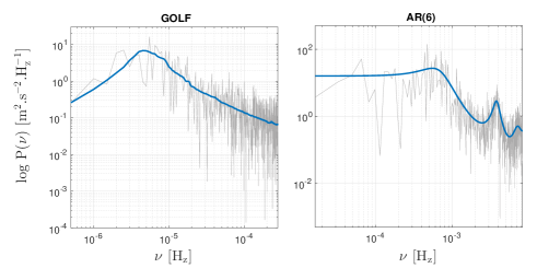
Figure 1: Left: Estimated PSD of the solar noise with part of GOLF data (blue) and periodogram of one of the $158$ data blocks (grey). Parameters: $N=1110$, $\Delta t=30$ min. This PSD is used to generate the noise for Figs. 2 and 4. Right: Theoretical PSD of the AR(6) noise (blue) and one noise periodogram (grey). This PSD is used for Fig. 3. Parameters:$N=1024$, $\Delta t=1$ min.

Under ${\cal{H}}_{1}$, several cases of exoplanetary RV signatures will be considered. The tests’ performances will be illustrated by ROC curves representing $\rm P_{DET}$ as a function of $\rm P_{FA}$. For Monte Carlo (MC) simulations, $10^{4}$ realizations have been used.

VII-B Analytical expressions for tests based on ${\bf\widetilde{\bf P}}\;|\;\overline{\bf P}_{L}$

We first consider the tests ${\rm T_{M}}({\bf\widetilde{\bf P}}\,|\,\overline{\bf P}_{L})$ and ${\rm T_{C}}({\bf\widetilde{\bf P}}\;|\;\overline{\bf P}_{L})$. The first panel of Fig.2 compares to empirical results obtained from MC simulations to the expressions obtained for the $\rm P_{FA}(\gamma)$ for both tests (see (18) and (22)). The second panel regards the corresponding expressions for $\rm P_{DET}(\gamma)$ ((19) and (23)) and the last panel the expression (LABEL:Eq20) for $\rm P_{DET}(P_{FA})$. All the theoretical expressions are shown by color dots and the empirical results from MC simulations are plotted in full lines. Different values of $L$ are considered to illustrate the improvement brought by larger training data sets. The figure shows a fair agreement between theoretical and empirical results, even for the not so large value of $N$ considered here (N = 1110). The test performances logically increase with $L$, as the estimation noise decreases with the increasing size of the training data set.

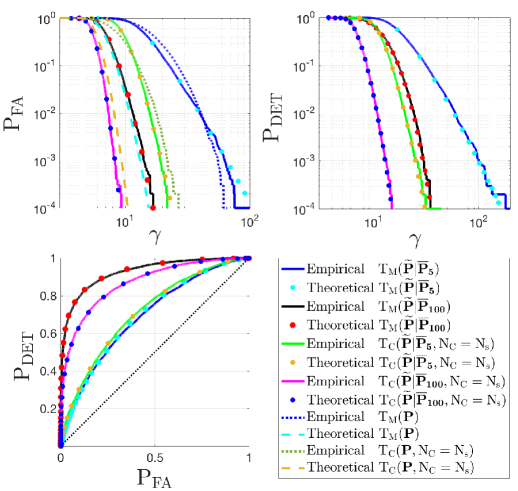
Figure 2: Theoretical vs empirical results for ${\rm T_{M}}({\bf\widetilde{\bf P}}\,|\,\overline{\bf P}_{L})$ and ${\rm T_{C}}({\bf\widetilde{\bf P}}\;|\;\overline{\bf P}_{L})$ by MC simulations. Parameters: $\Delta t=30$ min, $N_{s}=3$, $\alpha_{q}=0.2$ m.s^-1 for the three RV signatures of respective periods $11$ h, $2.45$ d and $6.61$ d. The curves in dashed lines show the inconsistency of ignoring noise correlations (Sec. VII-C).

VII-C Effects of standardization by $\overline{\bf P}_{L}$

We compare the detection performances of the tests ${\rm T_{M}}$ and ${\rm T_{C}}$ applied to the standardized periodogram $(\widetilde{\bf P}|\overline{\bf P}_{L})$ with their unstandardized versions ${\rm T_{M}}(\bf P)$ and ${\rm T_{C}}(\bf P)$, as described in Sec. IV-B. We evaluate first how accurate would be the false alarm rate obtained by neglecting noise correlation for tests ${\rm T_{C}}$ and ${\rm T_{M}}$. For this we assume the detectors consider the noise is white and have knowledge of $\sigma^{2}_{E}$, the exact variance of $E$. When ${\bf{Z}}=2{\bf{P}}/\sigma^{2}_{E}$, it is easy to show that the false alarm rates assumed by these two tests are given by

$$\!\!\!\!\left\{\begin{aligned} &{\rm P_{FA}}\left({\rm T_{M}}(2{\bf{P}}/\sigma^{2}_{E}),\gamma\right)=1-\Phi_{\chi^{2}_{2}}^{\frac{N}{2}-1}(\gamma),\\ &{\rm P_{FA}}\left({\rm T_{C}}(2{\bf{P}}/\sigma^{2}_{E},N_{C}),\gamma\right)=I_{\Phi_{\chi^{2}_{2}(\gamma)}}(N_{C},\frac{N}{2}-N_{C}).\end{aligned}\right.$$ (26)

These expressions are compared to the true false alarm rates in the top left panel of Fig. 2. The cyan dashed and blue dotted curves show respectively approximation (26) and empirical $\rm P_{FA}$ for ${\rm T_{M}}$, while the yellow dashed and red dotted curves show respectively approximation (26) and empirical $\rm P_{FA}$ for ${\rm T_{C}}$. Clearly, the correspondence between the thresholds values and the target false alarm rates is destroyed because of noise correlation in absence of standardization.

VII-D Effects of standardization by $\widehat{\bf S}_{E,AR}$

As discussed in Sec.VI, a way to deal with the frequency dependence of the noise is to estimate its PSD by parametric models. A difficulty with such methods is the injection of estimation noise in the detection process. A standard approach discussed in Sec.VI is to consider that the estimates are sufficiently accurate for their intrinsic error to be negligible. We study the performances of this approach here. For this we consider the case of five sinusoidal signals with frequencies falling into a ‘valley’ of the noise PSD (Fig.1, right panel). We assume the noise PSD follows an AR model (which is indeed the case here) and we estimate $\widehat{S}_{E,AR}$ as described in Sec.VI. The question is the reliability of tests using ${\bf\widetilde{\bf P}}\;|\;\widehat{\bf S}_{E,AR}$, and in particular how accurate is expression (LABEL:PFA_param) with this approach.

Fig.3 compares, as a function of the test threshold, the $\rm P_{FA}$ assumed by approximation (LABEL:PFA_param) (blue curve) with the actual false alarm rates obtained for $1000$ MC simulations.

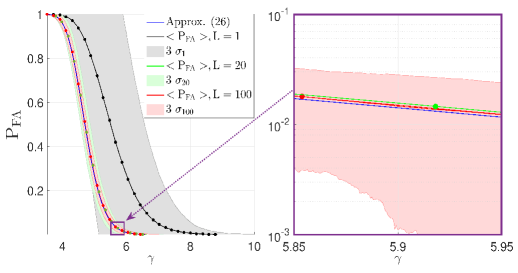
Figure 3: Comparison of the approximated $\rm P_{FA}$ (LABEL:PFA_param) (blue curve) with true $\rm P_{FA}$ for $L=1,20$ and $100$. The solid lines with dots represent the average actual $\rm P_{FA}$. The shaded regions are the corresponding $3\sigma$ enveloppes. The right panel is a zoom in log-scale on the violet square in left panel. Parameters: $N_{s}=5$, $\alpha_{q}=0.07$ m.s^-1, $f_{q}=[5.0,5.5,5.75,6,6.5]$ mHz.

In each such simulation, an estimate $\widehat{\bf S}_{E,AR}(L)$ was obtained with Akaike’s Final Prediction Error (FPE) [78] from $L$ noise time series and used to calibrate the periodogram. For each such estimate, the true $\rm P_{FA}$ of test ${\rm T_{C}}({\bf\widetilde{\bf P}}\;|\;{\widehat{\bf S}_{E,AR}},N_{C}=N_{s})$ was evaluated using 100 MC simulations. The figure plots, respectively for $L=1,20$ and $100$ the average $\rm P_{FA}$, respectively in black, green and red solid lines with dots. We see that (LABEL:PFA_param) is accurate, on average, only when $L$ is large. This figure also indicates the variability of the true false alarm rate. For each value of $L$, the figure shows the $3\sigma$ dispersion of the true $\rm P_{FA}$ w.r.t. its empirical average (shaded regions in grey for $L=1$, green for $L=20$ and red for $L=100$). Even when $N$ is large, the true significance levels at which such tests are conducted can undergo wild (and in practice unknown) variations. The right panel is a zoom on the $3\sigma$ region for $L=100$. For a threshold $\gamma=5.9$ for instance, the $\rm P_{FA}\approx 0.013$ from (LABEL:PFA_param). In the right panel, we see that the true false alarm rate for this threshold varies in reality in the range $[0.001\;0.3]$. For smaller values of $L$, the excursions of the true false alarm rates are so large that (LABEL:PFA_param) is simply useless. Conclusions drawn from tests based on parametric estimation may thus be very hazardous, even when the parametric model is true and when large data sets are available for PSD estimation.

VII-E ${\rm T_{C}}({\bf\widetilde{\bf P}}|\overline{\bf P}_{L},N_{C})$ and ${\rm T_{M}}({\bf\widetilde{\bf P}}|\overline{\bf P}_{L})$ vs adaptative approaches

We do not attempt to apply ${\rm HC^{\star}}$ and ${\rm BJ}$ to ${\bf{P}}$ in the correlated case as this leads to the same inconsistencies as those illustrated in Sec. VII-C and Fig. 2, top left panel, dotted curves. We compare here the adaptative approaches ${\rm HC^{\star}}$ and ${\rm BJ}$ standardized by $\overline{\bf P}_{L}$ as in Sec.V-D with the corresponding tests ${\rm T_{M}}$ and ${\rm T_{C}}$ for $L=1$ and $L=50$. (Note that when $N_{C}=1$, ${\rm T_{C}}$ reduces to ${\rm T_{M}}$, cf (13)).

For this comparison, we consider two different cases of Keplerian signals under $\mathcal{H}_{1}$, which are typical of ‘super-Earth’ planets (Fig. 4): $N_{p}=1$ planet with null eccentricity in Case 1 (left column), and $N_{p}=5$ eccentric planets in Case 2 (right column).

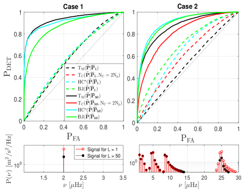
Figure 4: Top panels: Empirical ROC curves comparing classical and adaptative tests for different signals. Case 1: $N_{p}=1$, $M_{p}=3.5M_{\oplus}$ (for $L=1$), $T_{p}=5.7813$ d (signal frequency $1/T_{p}$ on-grid), $e_{p}=0$, $\omega_{p}=0$, $T_{0}=0$, $\gamma_{0}=0$. For $L=50$, $M_{p}=0.8M_{\oplus}$. Case 2: $N_{p}=5$, $M_{p}=[0.15,0.15,0.25,0.25,0.25]M_{\oplus}$ (for $L=1$), $T_{p}=[11.21~{}{\rm h},1.33~{}{\rm d},2.45~{}{\rm d},6.91~{}{\rm d},9.25~{}{\rm d}]$ (signal frequencies off-grid), $e_{p}=0.9$, $\omega_{p}=\pi$, $T_{0}=0$, $\gamma_{0}=0$. For $L=50$, $M_{p}(T_{p}=11.21~{}{\rm h})=0.07M_{\oplus}$. In the adaptative tests, $\alpha_{0}=1/2$. Bottom panels: periodograms (logscale) of the signals under ${\mathcal{H}}_{1}$.

The lower panels illustrate the periodogram of the (noiseless) Keplerian signatures for the two cases. We see the apparition of significant harmonics in the case of off-grid signal frequencies and highly eccentric orbits. For each case, the planet masses have been adapted depending on the considered value of $L$ for a better display of the ROC curves.

From $L=1$ (dashed lines) to $L=50$ (solid lines), the performances of all tests increase in both cases. When the signal is extremely sparse in the Fourier domain (Case 1), ${\rm T_{M}}$ is more powerful than the considered adaptive approaches. This situation changes when the spectrum is less sparse (Case 2, compare the bottom panels), which is expected.

Results of [49] show that for a proportion of deviations in the range $[(\frac{N}{2}-1)^{\frac{1}{4}}\;(\frac{N}{2}-1)^{\frac{1}{2}}]$ an adaptive procedure such as HC may have better asymptotic power than $\rm T_{M}$. For the case $N=1110$ considered here, this corresponds to the range $[5\;23]$ (considering $\Omega$). The situation should be opposite for very sparse signals (in the range $[1\;4]$ here). It turns out that the superiority of adaptive procedures is confirmed in Fig. 4, where the spectrum is $1$-sparse in Case 1 and about $10$-sparse in Case 2. Note, however, that while the theory of [49] may be used as a guideline for guessing the sparsity range in which each test should work better, we should not expect a too tight agreement with this theory. Indeed, in the framework of [49], all deviations under the alternative have the same amplitude, while RV signals lead to different amplitudes in general. Moreover, these theoretical results are asymptotical (while $N$ is not so large here).
An interesting point is the comparison of $\rm HC^{\star}$ and $\rm BJ$ with ${\rm T_{C}}({\bf\widetilde{\bf P}}|\overline{\bf P}_{L},N_{C})$, for which $N_{C}$ is a proxy for the number of significant deviations in the Fourier spectrum (here we considered $N_{C}=1$ in Case 1 and $N_{C}=10$ in Case 2). ${\rm T_{C}}$ represents a kind of Oracle, which knows in which region of the $P$-values to look at in order to ‘make the case’ against $\mathcal{H}_{0}$. The right panel shows that adaptive procedures have better power than ${\rm T_{C}}$, yet without prior knowledge.

VII-F A detectability study

A direct application of the previous results is detectability studies, which can be used for the design of observational strategies for instance. To illustrate this, we consider under $\mathcal{H}_{1}$ a planet with the parameters of $\alpha$ Centauri B’s exoplanet candidate as estimated in [16] (see the legend of Fig.5). As the eccentricity is supposed null, the signal can be considered very sparse in the Fourier domain. We consider the $\rm T_{M}$ test and a time sampling of $\Delta t=4$ hours. It was allowed to slightly vary from one value of $N$ to another in order to guarantee that the planet’s period yields a frequency exactly on the Fourier grid, in which case the spectrum is $1$-sparse on $\Omega$ and $\rm T_{M}$ is the test that yields the best performances.

As for the noise PSD, we used a model based on HD simulations of a star with similar spectral type as that of $\alpha$CenB. There is some mismatch between the simulated RV time series of the spectral type (G2) and the true spectral type (K1) of $\alpha$CenB. Because spectral type affects the noise properties [85], these results should not be considered to reflect perfectly the case of the candidate planet orbiting $\alpha$CenB.

In Fig.5, we illustrate the feasible performance compromises $(\rm P_{DET},\rm P_{FA})$ as a function of $N$, for three target $\rm P_{FA}$ ($0.5,\;0.1$ and $0.01$, indicated respectively by the dotted, solid and dashed lines) and for different sizes of available training data sets $L$ ($\infty,100,20,5$, shown respectively in black, green, blue and red). These curves were built using the expressions (20) and (LABEL:Eq20) for the ${\rm T_{M}}$ test and we checked that they are accurate in separate MC simulations (not shown). In the case $L\to+\infty$, we use the fact that $F(2,2L)\underset{L\to+\infty}{\longrightarrow}\chi_{2}^{2}$ to calculate the theoretical $\rm P_{DET}(P_{FA})$.

The study presented in Fig.5 allows to quantify interesting facts. First, of course, $\rm P_{DET}$ is larger if the allowed $\textrm{P}_{\textrm{FA}}$ is larger. Second, for a fixed $\textrm{P}_{\textrm{FA}}$, $\rm P_{DET}$ is larger for a larger value of $L$. Going to specific cases, we see that if a planet similar to the considered candidate was orbiting a star of the considered spectral type (G2), of which 100 training time series are available, it would require 250 days ($1500\times 4$h) of observations with 1 point every 4 hours to guarantee a probability of detection of $0.9$ while ensuring a false alarm rate of $0.01$. This situation is indicated by the black square. With only $L=5$ training time series, the probability of detection would fall to about $0.1$, all other parameters equal (red square).

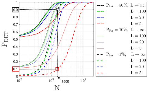
Figure 5: Example of a detectability study for a planet (relevant Keplerian parameters: $K=0.54$ m.s^-1, $T_{p}=3.23$ d and $e=0$; $M_{p}=1.241M_{\oplus}$, orbit inclination of $90\degree$, semi-major axis $a=0.0425$ Astronomical Unit) orbiting a G2 type star. The plot shows the achievable $\rm P_{DET}$ for different configurations of $\textrm{P}_{\textrm{FA}}$ budgets and numbers of available training light curves.

VIII Summary and perspectives

This paper has investigated the possibility of using training data sets to standardize periodograms in order to improve the control of the resulting false alarm rate. The paper first provided an extended (though unavoidably selective) overview of classical and recent techniques in sinusoid detection, with emphasis on the problem of designing CFAR detectors for the composite hypotheses of multiple sinusoids and colored noise. We proposed an asymptotic analysis of the periodograms statistics after standardization for a model involving an unknown number of sinusoids with unknown parameters in partially unknown colored noise. This analysis allowed to characterize the performances of some standardized tests in terms of false alarm and detection rates. We showed that when standardization is performed with a simple averaged periodogram as a noise PSD estimate these tests are CFAR for all sizes of training data sets. In contrast, we pointed out that standardization based on parametric estimates of the noise PSD may present actual false alarm rates that may be very far from the assumed ones, even for large data sets.
The tests we considered include classical approaches and also more recent adaptive tests designed for the rare and weak setting. For the latter tests, the standardization (by $\overline{\bf{P}}_{L}$) offers the same benefits as if the statistics of the noise were known a priori, with the CFAR property added. We also showed that such tests can present better power comparing to procedures for which the number of sinusoids would be known in advance.

In practical situations, some of the assumptions (i-iv) in Sec. I-A may not be met. This can be the case in exoplanet detection using RV time series, owing for instance to astrophysical effects linked to magnetic activity (like spots, affecting (i)) or instrumental defects / observational constraints (affecting (ii) and (iii)). Comparing theory to pratice, the present study is useful to make feasibility studies (as in Sec. VII-F), which then describe best achievable performances (i.e., around “quiet” stars and in absence of other unmodelled perturbations) for a regular sampling.

An important extension to the considered framework regards the case when, for periodicity analysis, the time series is not correlated to orthogonal exponentials. This case encompasses situations where (a) the sampling is irregular, (b) $P$ is not evaluated on the Fourier grid (as in oversampled periodograms) (c) $P$ is modified in the form of “generalized periodograms”, which correlate the time series with highly redundant dictionaries of specific features [28, 86, 87, 88, 89, 90, 91, 92, 93]. In such cases, the considered ordinates exhibit strong dependencies. With the additional complication of partially unknown colored noise, analytical evaluation of the false alarm rate for the considered tests seems out of reach. We conducted however preliminary studies suggesting that it might be possible to obtain accurate estimates of the false alarm rate when the noise is colored, the sampling irregular, the considered frequencies not restricted to Fourier grid and $N$ small, by combining the standardization proposed in the present paper with bootstrap procedures [94] and maximum likelihood estimation of Generalized Extreme Values distributions’ parameters [87, 95]. This numerical approach, still under study, would allow to address important questions, like that of the impact of the sampling distribution on the detection performances.

Appendix A Derivation of expressions (5) and (6)

We prove here that for model (3) the periodogram is asymptotically distributed as in (5) with non centrality parameters as in (6). The proof is adapted from Theorem 6.2 of [24], which considers the complex case. We first prove (5) and then turn to (6). The time series of model (3) can also be written as

$$X(j)=\sum_{q=1}^{N_{s}}\alpha_{q}\sin(2\pi f_{q}j+\varphi_{q})+E(j)=R(j)+E(j),$$

with $R(j):=\sum_{q=1}^{N_{s}}\alpha_{q}\sin(2\pi f_{q}j+\varphi_{q})$ a deterministic part, which using Euler formulae can be written as

$$R(j) =\sum_{q=1}^{N_{s}}\frac{\alpha_{q}}{2}\mathrm{e}^{{\rm{i}}(\varphi_{q}-\frac{\pi}{2})}\mathrm{e}^{2\pi{\rm{i}}f_{q}j}-\frac{\alpha_{q}}{2}\mathrm{e}^{-{\rm{i}}(\varphi_{q}+\frac{\pi}{2})}\mathrm{e}^{-2\pi{\rm{i}}f_{q}j}.$$

$$\vspace{-0.2cm}\!\!\!\!\!\!\!\!\text{By introducing:}~{}~{}~{}~{}~{}~{}\left\{\begin{aligned} &{\bf{f}}(\nu):=[\mathrm{e}^{{\rm{i}}2\pi\nu},\ldots,\mathrm{e}^{{\rm{i}}2\pi N\nu}]^{\top},\\ &{\bf{f}}^{+}(f_{q}):=\mathrm{e}^{{\rm{i}}(\varphi_{q}-\frac{\pi}{2})}{\bf{f}}(f_{q}),\\ &{\bf{f}}^{-}(f_{q}):=\mathrm{e}^{-{\rm{i}}(\varphi_{q}+\frac{\pi}{2})}{\bf{f}}(f_{q}),\end{aligned}\right.$$

the time series writes in vector form :

$${\bf{X}} ={\sum_{q=1}^{N_{s}}}\frac{\alpha_{q}}{2}\Big{(}{{{\bf{f}^{+}}(f_{q})}-{{\bf{f}^{-}}(f_{q})}}\Big{)}+{\bf{E}}={\bf{R}}+{\bf{E}}$$ (27)

and its discrete Fourier transform (DFT) $y_{k}$ at frequency $\nu_{k}$ is

$$y_{k}=\frac{1}{N}{\bf{f}}^{H}(\nu_{k}){\bf{X}}=\frac{1}{N}{\bf{f}}^{H}(\nu_{k}){\bf{R}}+\frac{1}{N}{\bf{f}}^{H}(\nu_{k}){\bf{E}}.$$

The DFT is composed of a deterministic part, ${\mu_{k}}$, and a stochastic part, ${\epsilon}_{k}$, defined as

$${\mu_{k}}:=\frac{1}{N}{\bf{f}}^{H}(\nu_{k}){\bf{R}}\quad{\textrm{and}}\quad{\epsilon}_{k}:=\frac{1}{N}{\bf{f}}^{H}(\nu_{k})\bf{E}.$$ (28)

Because $E$ is a zero mean Gaussian process, the random variable $y_{k}=\mu_{k}+\epsilon_{k}$ is Gaussian with mean $\mu_{k}$ and variance $\sigma^{2}_{k}$. This is a complex variable for all Fourier frequencies except for $\nu_{0}$ and $\nu_{\frac{N}{2}}$ because ${\bf{f}}(\nu_{0})$ and ${\bf{f}}(\nu_{\frac{N}{2}})$ are real.

The distribution of the periodogram requires to investigate the variance of $\epsilon_{k}$ which, with (28), writes:

$$N\textrm{var}{\;\epsilon_{k}}=\frac{1}{N}\mathbb{E}\;\left({\bf{f}}^{H}(\nu_{k}){\bf{E}}{\bf{E}}^{\top}{\bf{f}}(\nu_{k})\right)$$

$$=\frac{1}{N}{\sum_{t,s=1}^{N}}r_{E}(t-s)\mathrm{e}^{-{\rm{i}}2\pi\nu_{k}(t-s)}$$

$$=\frac{1}{N}{\sum_{|u|<N}}(N-|u|)r_{E}(u)\mathrm{e}^{-{\rm{i}}2\pi\nu_{k}u}$$

$$=S_{E}(\nu_{k})-\!\!\!{\sum_{|u|<N}}\frac{|u|}{N}r_{E}(u)\mathrm{e}^{-{\rm{i}}2\pi\nu_{k}u}-\!\!\!{\sum_{|u|\geq N}}r_{E}(u)\mathrm{e}^{-{\rm{i}}2\pi\nu_{k}u}$$

$$=S_{E}(\nu_{k})+{\mathcal{O}}(r_{N}),$$

since, using the absolutely summable autocorrelation function $\sum_{u}|r_{E}(u)|<\infty$ and the dominated convergence theorem we have

$$r_{N}:=\sum_{u}\min(1,\frac{|u|}{N})|r_{E}(u)|\to 0\textrm{\;\;as\;\;}N\to\infty.\vspace{-0.2cm}$$ (29)

Hence, for all Fourier frequencies,

$$\sigma^{2}_{k}:=\textrm{var}\;\epsilon_{k}=N^{-1}S_{E}(\nu_{k})+{\mathcal{O}}(N^{-1}r_{N}).$$ (30)

By Lemma 12.2.1(b) of [24], we obtain

$$|y_{k}|^{2}/\sigma^{2}_{k}\sim\left\{\begin{aligned} &{\frac{1}{2}}\chi^{2}_{2,2\frac{|\mu_{k}|^{2}}{\sigma^{2}_{k}}},~{}~{}~{}~{}\forall k~{}\in~{}\Omega,\\ &\chi^{2}_{1,\frac{|\mu_{k}|^{2}}{\sigma^{2}_{k}}},~{}\text{ for }~{}k=0,\frac{N}{2}.\end{aligned}\right.$$

Hence, for the periodogram this implies

$$P(\nu_{k}|H_{1}) =N|y_{k}|^{2}=N\sigma^{2}_{k}(|y_{k}|^{2}/\sigma^{2}_{k})$$ (31)

$$\sim\left\{\begin{aligned} &\frac{1}{2}\rho^{-1}_{k}S_{E}(\nu_{k})\chi_{2,2\rho_{k}\gamma_{k}}^{2},~{}\forall k~{}\in~{}\Omega,\\ &\rho^{-1}_{k}S_{E}(\nu_{k})\chi^{2}_{1,\rho_{k}\gamma_{k}},~{}\text{ for }~{}k=0,\frac{N}{2},\end{aligned}\right.$$

where

$$\rho_{k}:=S_{E}(\nu_{k})/(N\sigma^{2}_{k})\quad{\textrm{and}}\quad\gamma_{k}:=N|\mu_{k}|^{2}/S_{E}(\nu_{k}).$$ (32)

With (30), we see that

$$\rho_{k}=\frac{S_{E}(\nu_{k})}{S_{E}(\nu_{k})+{\mathcal{O}(r_{N})}}=1+{\mathcal{O}(r_{N})}$$ (33)

for all Fourier frequencies. Owing to (29), an approximated distribution of (31) can be obtained by neglecting the $\mathcal{O}(r_{N})$ in (33). The distribution (5) follows by noting

$$\lambda_{k}:=2\gamma_{k}\;\;\text{for}\;\;k~{}\in~{}\Omega\quad\text{and}\quad\lambda_{k}:=\gamma_{k}\;\;\text{for}\;\;k=0,\frac{N}{2}.$$ (34)

We now turn to the computation of the non centrality parameters. We have from (27), (28) and (32)

$$\gamma_{k} =\frac{N}{S_{E}(\nu_{k})}|\frac{1}{N}{\bf{f}}^{H}(\nu_{k})\bf{R}|^{2}$$ (35)

$$=\frac{1}{NS_{E}(\nu_{k})}\Big{|}\sum_{j=1}^{N}\sum_{q=1}^{N_{s}}\frac{\alpha_{q}}{2}\Big{(}\mathrm{e}^{{\rm{i}}(\varphi_{q}-\frac{\pi}{2})}\mathrm{e}^{2\pi{\rm{i}}(f_{q}-\nu_{k})j}\!$$

$$~{}~{}~{}~{}~{}~{}~{}~{}~{}~{}~{}~{}~{}~{}~{}~{}~{}~{}~{}~{}~{}~{}~{}~{}~{}~{}\ldots-\!\mathrm{e}^{-{\rm{i}}(\varphi_{q}+\frac{\pi}{2})}\mathrm{e}^{-2\pi{\rm{i}}(f_{q}+\nu_{k})j}\Big{)}\Big{|}^{2}\!.$$

Introducing the Dirichlet Kernel (cf Lemma 12.1.3 of [24]):

$$D_{N}(\nu):=\frac{1}{N}\sum_{j=1}^{N}\mathrm{e}^{{\rm{i}}2\pi\nu j}=\frac{\sin(N\pi\nu)}{N\sin(\pi\nu)}\mathrm{e}^{{\rm{i}}(N+1)\pi\nu},$$

and the corresponding Fejér kernel (or spectral window)

$$K_{N}(\nu):=|D_{N}(\nu)|^{2}=\Bigg{(}\frac{\sin(N\pi\nu)}{N\sin(\pi\nu)}\Bigg{)}^{2},$$ (36)

expression (35) becomes

$$\gamma_{k} =\frac{N}{4S_{E}(\nu_{k})}\Big{|}\sum_{q=1}^{N_{s}}\alpha_{q}\Big{(}D_{N}(f_{q}-\nu_{k})\mathrm{e}^{{\rm{i}}(\varphi_{q}-\frac{\pi}{2})}$$

$$~{}~{}~{}~{}~{}~{}~{}~{}~{}~{}~{}~{}~{}~{}~{}~{}~{}~{}~{}~{}~{}~{}~{}~{}~{}~{}~{}~{}~{}~{}~{}~{}~{}~{}~{}~{}\ldots-D_{N}(f_{q}+\nu_{k})\mathrm{e}^{-{\rm{i}}(\varphi_{q}+\frac{\pi}{2})}\!\Big{)}\!\Big{|}^{2}.$$

This equation can also be written as :

$$\gamma_{k}=\frac{N}{4S_{E}(\nu_{k})}\Big{|}\sum_{q=1}^{N_{s}}\alpha_{q}z_{q}(\nu_{k})\Big{|}^{2},$$ (37)

with

$$z_{q}(\nu_{k}) :=D_{N}(f_{q}-\nu_{k})\mathrm{e}^{{\rm{i}}(\varphi_{q}-\frac{\pi}{2})}\!-\!D_{N}(f_{q}+\nu_{k})\mathrm{e}^{-{\rm{i}}(\varphi_{q}+\frac{\pi}{2})}$$ (38)

$$=x_{+}\mathrm{e}^{{\rm{i}}\theta_{+}}-x_{-}\mathrm{e}^{{\rm{i}}\theta_{-}}$$

$$=(x_{+}\cos\theta_{+}-x_{-}\cos\theta_{-})+{\rm{i}}(x_{+}\sin\theta_{+}-x_{-}\sin\theta_{-}),$$

where

$$\left\{\begin{aligned} x_{+}&=x_{+}\left({\nu_{k}},q\right):=\frac{\sin(N\pi(f_{q}-\nu_{k}))}{N\sin(\pi(f_{q}-\nu_{k}))},\\ x_{-}&=x_{-}\left({\nu_{k}},q\right):=\frac{\sin(N\pi(f_{q}+\nu_{k}))}{N\sin(\pi(f_{q}+\nu_{k}))},\\ \theta_{+}&=\theta_{+}\left({\nu_{k}},q\right):=+[(N+1)\pi(f_{q}-\nu_{k})+(\varphi_{q}-\frac{\pi}{2})],\\ \theta_{-}&=\theta_{-}\left({\nu_{k}},q\right):=-[(N+1)\pi(f_{q}+\nu_{k})+(\varphi_{q}+\frac{\pi}{2})].\\ \end{aligned}\right.$$

The modulus $\kappa_{q}$ of $z_{q}$ may be written as

$$\kappa_{q}:=|z_{q}|=\left(x_{+}^{2}+x_{-}^{2}-2x_{+}x_{-}\cos{(\theta_{+}-\theta_{-})}\right)^{\frac{1}{2}},$$ (39)

$$\text{with}~{}~{}~{}~{}~{}~{}~{}~{}~{}\left\{\begin{aligned} x_{+}^{2}&=K_{N}(f_{q}-\nu_{k}),\\ x_{-}^{2}&=K_{N}(f_{q}+\nu_{k}),\\ \theta_{+}-\theta_{-}&=2\pi(N+1)f_{q}+2\varphi_{q},\end{aligned}\right.$$

$$\text{and}~{}~{}~{}~{}~{}~{}~{}~{}~{}~{}~{}~{}~{}~{}~{}~{}~{}\theta_{q}:=\angle\;z_{q},\;\theta_{q}\;\in\;]-\pi,\pi],$$ (40)

the phase of $z_{p}$ obtained from the real and imaginary parts of (38) [96]. With these notations, it is easy to show that

$$\Big{|}\sum_{q=1}^{N_{s}}z_{q}\Big{|}^{2}=\sum_{q=1}^{N_{s}}\Big{[}\kappa_{q}^{2}+2\kappa_{q}\sum_{\ell=q+1}^{N_{s}}\kappa_{\ell}\cos(\theta_{q}-\theta_{\ell})\Big{]}~{}~{}\text{for $N_{s}>1$}.$$

Consequently, the expression of the $\{\gamma_{k}\}$ in (37) becomes

$$\gamma_{k}\!=\!\frac{N}{4S_{E}(\nu_{k})}\!\!\sum_{q=1}^{N_{s}}\!\!\Big{[}\alpha_{q}^{2}\kappa_{q}^{2}\!\!+\!2\alpha_{q}\kappa_{q}\!\!\sum_{\ell=q+1}^{N_{s}}\!\!\!\alpha_{\ell}\kappa_{\ell}\!\cos(\theta_{q}-\theta_{\ell})\Big{]}$$ (41)

and the non centrality parameters $\{\lambda_{k}\}$ of (6) follow from (34),with $\kappa_{q}$ and $\theta_{q}$ given by (39) and (40). $\hfill\square$

Note that if all signal frequencies $\{f_{p}\}$ fall on the Fourier frequency grid, the crossed term in (41) vanish owing to the orthogonality of the Fejér kernels centered at different signal frequencies. In this case, expression (41) precisely reduces to expression given in Remark 6.6 of [24].

We finally wish to mention that the expression of the non centrality parameters is erroneously reported in exp. (5) of [55] (sign error and crossed terms missing).

Appendix B Derivation of expression (23)

Let $K$ denote the number of ordinates of ${\bf\widetilde{\bf P}}\;|\;\overline{\bf P}_{L}$ larger than $\gamma$ under $\mathcal{H}_{1}$, and $p_{i}:=\textrm{Pr}\;(K=i\;|\;{\cal{H}}_{1})$. From the definition (13), we have:

$$\!\!\rm{P_{DET}}({T}_{C}({\bf\widetilde{\bf P}}|\overline{\bf P}_{L}),\gamma,N_{C})\!:=\!\textrm{Pr}\;({T_{C}({\bf\widetilde{\bf P}}|\overline{\bf P}_{L},N_{C})}\!\!>\!\gamma|{\cal{H}}_{1}\!)\!$$ (42)

$$=\textrm{Pr}\;(K\geq N_{C}\;|\;{\cal{H}}_{1})$$

$$=1-{\sum_{i=0}^{N_{C}-1}}\textrm{Pr}\;(K=i\;|\;{\cal{H}}_{1})=1-{\sum_{i=0}^{N_{C}-1}}p_{i}.$$

Owing to (10) each ordinate $({\bf\widetilde{\bf P}}|\overline{\bf P}_{L})_{i}:=\frac{\widetilde{P}(\nu_{i})}{\overline{P}_{L}(\nu_{i})}$ has probability $1-\Phi_{F_{\lambda_{i}}}(\gamma)$ to be larger than $\gamma$. These variates can be considered approximately independent but not i.i.d. Hence, the variable $K$ is not binomially distributed (as it is under ${\cal{H}}_{0}$) and the probabilities $\{p_{i}\}$ require further investigation. We proceed by induction. In the following, all probabilities are under $\mathcal{H}_{1}$. The first probability $p_{0}$ can simply be approximated as

$$p_{0}=\textrm{Pr}\left\{\bigcap_{k=1}^{\frac{N}{2}-1}({\bf\widetilde{\bf P}}\;|\;\overline{\bf P}_{L})_{k}\leq\gamma\right\}\approx{\prod_{k=1}^{\frac{N}{2}-1}}\Phi_{F_{\lambda_{k}}}.$$

The probability $p_{1}=\text{Pr}(K=1)$ is similarly

$$p_{1} =\textrm{Pr}{\displaystyle{\bigcup_{k=1}^{\frac{N}{2}-1}}}\left\{({\bf\widetilde{\bf P}}\;|\;\overline{\bf P}_{L})_{k}>\gamma\bigcap_{j\neq k}({\bf\widetilde{\bf P}}\;|\;\overline{\bf P}_{L})_{j}\leq\gamma\right\}$$

$$\approx{\sum_{k=1}^{\frac{N}{2}-1}\Big{[}(1-\Phi_{F_{\lambda_{k}}})\displaystyle{\prod_{\begin{subarray}{c}j=1,\\ j\neq k\end{subarray}}^{\frac{N}{2}-1}}\Phi_{F_{\lambda_{j}}}\Big{]}}.$$

To generalize further, denote by ${\Omega}^{(i)}$ one particular combination of $i$ indices taken in $\Omega$ and $\overline{\Omega}^{(i)}:=\Omega\backslash\Omega^{(i)}$ the set of remaining indices. Let $\{\Omega^{(i)}_{1},\ldots,\Omega^{(i)}_{i}\}$ (resp. $\{\overline{\Omega}^{(i)}_{1},\ldots,\overline{\Omega}^{(i)}_{\frac{N}{2}-1-i}\}$) denote the indices in two such combinations, and let $\Omega^{i}$ be the set of all the $\{{\Omega}^{(i)}\}$. With these notations we obtain for $i>1$ :

$$p_{i} =\textrm{Pr}\!\!\!{\displaystyle{\bigcup_{{\Omega}^{(i)}\in{\Omega}^{i}}}}\left\{\bigcap_{k=1}^{i}({\bf\widetilde{\bf P}}\;|\;\overline{\bf P}_{L})_{\Omega^{(i)}_{k}}>\gamma\bigcap_{k^{\prime}=1}^{\frac{N}{2}-1-i}({\bf\widetilde{\bf P}}\;|\;\overline{\bf P}_{L})_{\overline{\Omega}^{(i)}_{k^{\prime}}}\leq\gamma\right\}$$ (43)

$$\approx{\sum_{\Omega^{(i)}}\prod_{k=1}^{i}}\Big{(}\!1\!-\Phi_{F_{\lambda_{\Omega^{(i)}_{k}}}\!\!^{\!\!\!\!\!\!\!\!\!(\gamma,2,2L)}}\!\!\Big{)}{\prod_{k^{\prime}=1}^{\frac{N}{2}-1-i}}\Phi_{F_{\lambda_{\overline{\Omega}^{(i)}\!_{\!\!\!\!\!\!k^{\prime}}}}{(\gamma,2,2L)}}.$$

Expression (23) follows by combining (42) and (43). $\hfill\square$

References

- [1] A. Schuster, “On the investigation of hidden periodicities,” J. Geophys. Res., vol. 3, pp. 13, 1898.
- [2] D.R. Brillinger, Time Series : Data Analysis and Theory, Holden Day, San Francisco, 1981.
- [3] M.S. Bartlett, “Periodogram analysis and continuous spectra,” Biometrika, vol. 37, pp. 1–16, 1950.
- [4] U. Grenander and M. Rosenblatt, Statistical analysis of stationary time series, John Wiley and Sons, 1957.
- [5] M.B. Priestley, Spectral Analysis and Time Series, Academic Press, San Diego, 1981.
- [6] P.J. Brockwell and R.A. Davis, Time series : theory and methods, Springer, 1991.
- [7] P. Bloomfield, Fourier Analysis of Time Series, Wiley-Intersci., 2000.
- [8] P. Stoica and R. Moses, Spectral analysis of signals, Prentice Hall, 2005.
- [9] B. G. Quinn and E.J. Hannan, The Estimation and Tracking of Frequency, Cambridge Univ., 2001.
- [10] F. Pepe et al., “Instrumentation for the detection and characterization of exoplanets,” Nature, vol. 513, pp. 358–366, 2014.
- [11] N.M. Batalha, “Exploring exoplanet populations with NASA’s Kepler Mission,” Proc. Nat. Acad. Sci., vol. 111, pp. 12647–12654, Sept. 2014.
- [12] M. Auvergne et al., “The CoRoT satellite in flight: description and performance,” A&A, vol. 506, pp. 411–424, 2009.
- [13] H. Rauer et al., “The PLATO 2.0 mission,” Experimental Astronomy, vol. 38, pp. 249–330, 2014.
- [14] D.A. Fischer et al., “Exoplanet Detection Techniques,” Protostars and Planets VI, pp. 715–737, 2014.
- [15] M. Perryman, The exoplanet handbook, Cambridge Univ., 2011.
- [16] X. Dumusque et al., “An Earth-mass planet orbiting Centauri B,” Nature, vol. 491, pp. 207–211, 2012.
- [17] A. Hatzes, “The Radial Velocity Detection of Earth-mass Planets in the Presence of Activity Noise: The Case of Centauri Bb,” ApJ, vol. 770, pp. 133, 2013.
- [18] V. Rajpaul et al., “Ghost in the time series: no planet for Alpha Cen B,” MNRAS, vol. 456, pp. L6–L10, 2016.
- [19] L. Bigot et al., “The diameter of the CoRoT target HD 49933,” A&A, vol. 534, no. 3, 2011.
- [20] R.A. Fisher, “Tests of Significance in Harmonic Analysis,” Proc. R. Soc. London, Ser. A, vol. 125, pp. 54–59, 1929.
- [21] S.T. Chiu, “Detecting periodic components in a white gaussian time series,” J. R. Stat. Soc. Series B, vol. 51, no. 2, pp. 249–259, 1989.
- [22] M. Shimshoni, “On fisher’s test of significance in harmonic analysis,” Geophys. J. R. Astronom. Soc., pp. 373–377, 1971.
- [23] S. Kay, “Adaptive detection for unknown noise power spectral densities,” IEEE Trans. Signal Process, vol. 47, no. 1, pp. 10–21, 1999.
- [24] T.H. Li, Time series with mixed spectra, CRC Press, 2014.
- [25] P. Whittle, “The simultaneous estimation of a time series harmonic components and covariance structure,” Trabajos de Estadistica, vol. 3, no. 1-2, pp. 43–57, 1952.
- [26] M.S. Bartlett, “An introduction to stochastic processes,” Quart. J. R. Meteorological Soc., vol. 81, no. 350, pp. 650, 1955.
- [27] A. Siegel, “Testing for periodicity in a time series,” J. Amer. Stat. Assoc., vol. 75, no. 370, pp. 345–348, 1980.
- [28] E. Bölviken, “New tests of significance in periodogram analysis,” Scandinavian J. Stat., vol. 10, no. 1, pp. 1–9, 1983.
- [29] E. Bölviken, “The distribution of certain rational functions of order statistics from exponential distributions,” Scandinavian J. Stat., vol. 10, no. 2, pp. 117–123, 1983.
- [30] R. Von Sachs, “Estimating the spectrum of a stochastic process in the presence of a contaminating signal,” IEEE Trans. Signal Process., vol. 41, no. 1, pp. 323, 1993.
- [31] R. Von Sachs, “Peak-insensitive non-parametric spectrum estimation,” J. Time Series Anal., vol. 15, no. 4, pp. 429–452, 1994.
- [32] R.J. Bhansali, “A mixed spectrum analysis of the lynx data,” J. R. Stat. Soc. Ser. A, , no. 142, pp. 199–209, 1979.
- [33] B. Truong-Van, “A new approach to frequency analysis with amplified harmonics,” J. R. Stat. Soc. Ser. B, vol. 52, pp. 203–221, 1990.
- [34] B.G. Quinn and J.M. Fernandes, “A fast efficient technique for the estimation of frequency,” Biometrika, vol. 78, no. 3, pp. 489–497, 1991.
- [35] B.G. Quinn, “A fast efficient technique for the estimation of frequency: Interpretation and generalisation,” Biometrika, vol. 86, pp. 213–220, 1999.
- [36] L. Kavalieris and Hannan E.J., “Determining the number of terms in a trigonometric regression.,” J. Time Series Analysis, vol. 15, pp. 613–625, 1994.
- [37] E.J. Hannan, “Testing for a jump in the spectral function,” J. R. Stat. Soc. Ser. B, vol. 23, no. 2, pp. 394–404, 1961.
- [38] D.F. Nicholls, “Estimation of the spectral density function when testing for a jump in the spectrum,” Austr. J. Stat., vol. 9, pp. 103–108, 1967.
- [39] S.T. Chiu, “Peak-insensitive parametric spectrum estimation,” Stochastic Processes and their Applications, vol. 35, pp. 121–140, 1990.
- [40] J.K. Gryca, “Detection of multiple sinusoids buried in noise via balanced model truncation,” IEEE Instrum. Meas. Conf., pp. 1353–1358, 1998.
- [41] L.B. White, “Detection of sinusoids in unknown coloured noise using ratios of ar spectrum estimates,” Proc. Inform., Decision and Control, pp. 257–262, 1999.
- [42] N. Lu and D. Zimmerman, “Testing for directional symmetry in spatial dependence using the periodogram,” J. Stat. Planning and Inference, vol. 129, pp. 369–385, 2005.
- [43] A.P. Liavas et al., “A periodogram-based method for the detection of steady-state visually evoked potentials.,” IEEE Trans. Biom. Eng., vol. 45, no. 2, pp. 242–248, 1998.
- [44] C. Zheng, “Detection of multiple sinusoids in unknown colored noise using truncated cepstrum thresholding and local signal-to-noise-ratio,” Applied Acoust., pp. 809–816, 2012.
- [45] B. Nadler and A. Kontorovich, “Model selection for sinusoids in noise: Statistical analysis and a new penalty term,” IEEE Trans. Signal Process., vol. 59, no. 4, pp. 1333–1345, 2011.
- [46] C. Koen, “The analysis of indexed astronomical time series - xi. the statistics of oversampled white noise periodograms,” MNRAS, vol. 449, no. 1, pp. 1098–1105, 2015.
- [47] C. Koen, “The analysis of indexed astronomical time series - xii. the statistics of oversampled fourier spectra of noise plus a single sinusoid,” MNRAS, vol. 453, no. 2, pp. 1793–1798, 2015.
- [48] M. Tuomi et al., “Signals embedded in the radial velocity noise. Periodic variations in the Ceti velocities,” A&A, vol. 551, pp. A79, 2012.
- [49] D. Donoho and J. Jin, “Higher criticism for detecting sparse heterogeneous mixtures,” Ann. Stat., 2004.
- [50] Y.I. Ingster et al., “Detection boundary in sparse regression,” Electron. J. Statist., vol. 4, pp. 1476–1526, 2010.
- [51] G. Walther, “The Average Likelihood Ratio for Large-scale Multiple Testing and Detecting Sparse Mixtures,” IMS Collections : From Probability to Stat. and Back: High-Dimensional Models and Processes, vol. 9, pp. 317–326, 2012.
- [52] A. Moscovich et al., “On the exact Berk-Jones statistics and their p-value calculation,” Electron. J. Stat., vol. 10, pp. 2329–2354, 2016.
- [53] V. Gontscharuk et al., “Goodness of fit tests in terms of local levels with special emphasis on higher criticism tests,” Bernoulli, vol. 22, no. 3, pp. 1331–1363, 2016,.
- [54] P. Hall and J. Jin, “Innovated higher criticism for detecting sparse signals in correlated noise,” Ann. Stat., vol. 38, pp. 1686–1732, 2010.
- [55] S. Sulis, D. Mary, and L. Bigot, “Using hydrodynamical simulations of stellar atmospheres for periodogram standardization: Application to exoplanet detection,” in IEEE ICASSP, March 2016, pp. 4428–4432.
- [56] S.K. Gupta et al., “UPSO three channel fast photometer,” Bulletin Astron. Soc. of India, vol. 29, pp. 479–486, 2001.
- [57] S. Sulis, D. Mary, and L. Bigot, “Overcoming the stellar noise barrier for the detection of telluric exoplanets: an approach based on hydrodynamical simulations,” in EAS Publications Series, D. Mary et al., Eds., Sept. 2016, vol. 78-79, pp. 247–274.
- [58] J.G. Proakis and D.G. Manolakis, Digital Signal Processing, Prentice-Hall, 1996.
- [59] M. Abramowitz et al., Spectral Analysis and Time Series, Dover Publications, 1972.
- [60] H.A. David and H.N. Nagaraja, Order Statistics, 3rd Ed., Wiley, 2003.
- [61] S.M. Kay, Fundamentals of Statistical signal processing. Vol II : Detection theory., Prentice-Hall, Inc, 1998.
- [62] B. G. Quinn, “Testing for the presence of sinusoidal components,” J. Appl. Probability, vol. 23, pp. 201–210, 1986.
- [63] A. Schwarzenberg-Czerny, “The distribution of empirical periodograms: Lomb–Scargle and PDM spectra,” MNRAS, vol. 301, pp. 831–840, 1998.
- [64] T. Aittokallio et al., “Testing for Periodicity in Signals: An Application to Detect Partial Upper Airway Obstruction during Sleep,,” J. Theoretical Medicine, vol. 3, no. 4, pp. 231–245, 2001.
- [65] J. Gutiérrez-Soto et al., “Low-amplitude variations detected by CoRoT in the B8IIIe star HD 175869,” A&A, vol. 506, pp. 133–141, 2009.
- [66] S. Aldor-Noiman et al., “The power to see: A new graphical test of normality.,” Am. Stat., vol. 68, no. 4, pp. 318–318, 2013.
- [67] D. Mary and A. Ferrari, “A non-asymptotic standardization of binomial counts in higher criticism,” in Inform. Theory (ISIT), IEEE Int. Symp., June 2014, pp. 561–565.
- [68] D.M. Kaplan and M. Goldman, “True equality (of pointwise sensitivity) at last: a dirichlet alternative to Kolmogorov-Smirnov inference on distributions.,” Tech. report, 2014.
- [69] V. Gontscharuk et al., “The intermediates take it all: Asymptotics of higher criticism statistics and a powerful alternative based on equal local levels.,” Biom. J., vol. 57, no. 1, pp. 159–180, 2014.
- [70] J. Li and D. Siegmund, “Higher criticism: -values and criticism,” Ann. Statist., vol. 43, no. 3, pp. 1323–1350, 2015.
- [71] R.H. Berk and D.H. Jones, “Goodness-of-fit test statistics that dominate the Kolmogorov statistics,” Z. Wahrscheinlichkeit., vol. 47, pp. 47–59, 1979.
- [72] A. Moscovich-Eiger and B. Nadler, “Fast calculation of boundary crossing probabilities for Poisson processes,” ArXiv e-prints (V.3), 2015.
- [73] J. Fan and Q. Yao, Nonlinear Time Series-Nonparametric and Parametric Methods, Springer-Verlag New York, 2003.
- [74] K. F. Turkman and A. M. Walker, “On the asymptotic distributions of maxima of trigonometric polynomials with random coefficients,” Advances in Applied Probability, vol. 16, no. 4, pp. 819–842, 1984.
- [75] R.A Davis and T. Mikosch, “The maximum of the periodogram of a non-gaussian sequence,” Ann. of Prob., vol. 27, pp. 522–536, 1999.
- [76] D. Rife and R. Boorstyn, “Single tone parameter estimation from discrete-time observations,” IEEE Trans. Inf. Theory, vol. 20, no. 5, pp. 591–598, 1974.
- [77] B.G. Quinn and P. J. Kootsookos, “Threshold behavior of the maximum likelihood estimator of frequency,” IEEE Trans. Signal Process., vol. 42, no. 11, pp. 3291–3294, 1994.
- [78] H. Akaike, “Fitting autoregressive models for prediction,” Ann. Inst. Stat. Math., vol. 21, no. 1, pp. 243–247, 1969.
- [79] H. Akaike, “A new look at the statistical model identification,” IEEE Trans. Automatic Control, vol. 19, no. 6, pp. 716–723, 1974.
- [80] E. Parzen, “Multiple time series: determining the order of approximating autoregressive schemes,” Tech. Report, , no. 23, pp. 716–723, 1975.
- [81] E.J. Hannan and B.G. Quinn, “The determination of the order of an autoregression,” J. R. Stat. Soc. Ser. B, vol. 41, pp. 190–195, 1979.
- [82] J. Rissanen, “Universal coding, information prediction and estimation,” IEEE Trans. Inf. Theory, , no. 30, pp. 629–636, 1984.
- [83] A. Boardman et al., “A study on the optimum order of autoregressive models for heart rate variability,” Physio. Meas., vol. 23, pp. 325, 2002.
- [84] R.A. Garcia et al., “Global solar Doppler velocity determination with the GOLF/SoHO instrument,” A&A, vol. 442, pp. 385–395, 2005.
- [85] N. Meunier et al., “Variability of stellar granulation and convective blueshift with spectral type and magnetic activity. I. K and G main sequence stars,” ArXiv e-prints, 2016.
- [86] R.V. Baluev, “Assessing the statistical significance of periodogram peaks,” MNRAS, vol. 385, pp. 1279–1285, 2008.
- [87] M. Süveges, “Extreme-value modelling for the significance assessment of periodogram peaks,” MNRAS, vol. 440, no. 3, pp. 2099–2114, 2014.
- [88] J.D. Scargle, “Studies in astronomical time series analysis. II - Statistical aspects of spectral analysis of unevenly spaced data,” ApJ, vol. 263, pp. 835–853, 1982.
- [89] G.L. Bretthorst, “Frequency Estimation And Generalized Lomb-Scargle Periodograms.,” Stat. Challenges in Astronomy, pp. 309–329, 2003.
- [90] T. Thong et al., “Lomb-wech periodogram for non-uniform sampling,” Proc. 26th Annu. Int. Conf. IEEE EMBS, 2004.
- [91] M. Zechmeister and M. Kürster, “The generalised Lomb-Scargle periodogram. A new formalism for the floating-mean and Keplerian periodograms,” A&A, vol. 496, pp. 577–584, 2009.
- [92] R.V. Baluev, “Keplerian periodogram for Doppler exoplanet detection: optimized computation and analytic significance thresholds,” MNRAS, vol. 446, pp. 1478–1492, 2015.
- [93] P.C. Gregory, “An apodized kepler periodogram for separating planetary and stellar activity signals,” MNRAS, vol. 458, pp. 2604–2633, 2016.
- [94] A.M. Zoubir, “Bootstrap: theory and applications,” in SPIE Conf., F.T. Luk, Ed., 1993, vol. 2027, pp. 216–235.
- [95] M. Süveges et al., “A comparative study of four significance measures for periodicity detection in astronomical surveys,” MNRAS, vol. 450, no. 2, pp. 2052–2066, 2015.
- [96] H.S. Kasana, Complex variables : theory and applications. 2nd Edition, Prentice-Hall of India, 2005.