Incoherence of Partial-Component Sampling in multidimensional NMR

Abstract

In NMR spectroscopy, undersampling in the indirect dimensions causes reconstruction artifacts whose size can be bounded using the so-called coherence. In experiments with multiple indirect dimensions, new undersampling approaches were recently proposed: random phase detection (RPD) [1] and its generalization, partial component sampling (PCS) [2]. The new approaches are fully aware of the fact that high-dimensional experiments generate hypercomplex-valued free induction decays; they randomly acquire only certain low-dimensional components of each high-dimensional hypercomplex entry. We provide a classification of various hypercomplex-aware undersampling schemes, and define a hypercomplex-aware coherence appropriate for such undersampling schemes; we then use it to quantify undersampling artifacts of RPD and various PCS schemes.

1 Introduction

In traditional NMR spectroscopy, the complete dataset covers a grid $(t_{1},\dots,t_{d})$, where $t_{d}$ varies along the direct (a.k.a acquisition) time dimension and $(t_{1},\dots,t_{d-1})$ along the indirect time dimensions, which are sampled parametrically by separate experiments. Following [3], many researchers achieved acceptable reconstruction with non-uniform sampling (NUS), in which they acquired only a scattered subset of the indirect times. Typically the undersampling scheme involved either random uniform sampling or Poisson sampling with an exponentially decaying rate function[4]. In many cases an NUS experiment can save a great deal of experiment time, while still producing an acceptable result.

Reconstructions from undersampled data will in general display artifacts, and it is important to understand and quantify them in order to know if the reconstructions are acceptable despite undersampling. Coherence provides a useful bound on the size of undersampling artifacts; it has been applied in NMR spectroscopy and MR imaging [4, 5], and in the mathematical study of compressed sensing [6, 7, 8]. Conceptually, coherence bounds the extent to which a point mass in the true underlying spectrum at any one $k$-tuple can generate apparent mass in the reconstruction at some other $k^{\prime}\neq k$. By controlling coherence we keep artifacts small. In fields outside NMR spectroscopy, signals are either real or complex valued, and acceptable definitions of coherence have been proposed and applied. However, these definitions are not specifically adopted for the NMR spectroscopy.

When States-Haberkorn-Ruben phase-sensitive detection (PSD) [9] is employed for frequency sign discrimination in the indirect dimensions, the complete data at each $t$-tuple $(t_{1},\dots,t_{d})$ in a $d$-dimensional experiment are $2^{d}$-dimensional hypercomplex numbers produced by $2^{d-1}$ complex reads. The required algebra of such hypercomplex numbers has been described in detail by Delsuc [10]. NUS can be applied in a fashion that is ignorant of the hypercomplex structure, and the traditional definition of coherence can be straightforwardly generalized for NUS in the hypercomplex case.

Recently, novel hypercomplex-aware undersampling schemes were proposed for the multidimensional case; for example, in a $d$-dimensional experiment, RPD [1] acquires at a given $t$-tuple only a single complex measurement rather than all $2^{d-1}$ complex reads. More generally, PCS [2] acquires at a given $t$-tuple, $2m$ components of a hypercomplex datum produced by $1\leq m\leq 2^{d-1}$ complex reads. In the most general PCS scheme, the number of components being sampled may even jump around somewhat randomly between $t$-tuples. To understand the artifacts caused by such undersampling, this paper formulates a hypercomplex-aware definition of coherence. This new definition, although somewhat more involved than the traditional non-hypercomplex-aware quantity, seems to be the right notion for studying RPD and PCS because it obeys the core exact-reconstruction result that one wants coherence to obey: As we show here, a sufficiently low coherence allows a sufficiently sparse spectrum to be recovered correctly by convex optimization.

2 Approaches to Undersampling in NMR

We call each specific tuple $(t_{1},t_{2},\dots,t_{d-1})$ of indirect sampling times an indel (for indirect element). Associated with each indel is a hypercomplex-valued free induction decay (FID) $f_{t_{1},\dots,t_{d-1}}=\{f_{t_{1},\dots,t_{d-1}}(t_{d}):0\leq t_{d}<T_{d}\}$. Each hypercomplex entry $f_{t_{1},\dots,t_{d-1}}(t_{d})$ can be represented - see farther below - as a tuple of $m=2^{d-1}$ complex numbers $f=(f^{1},\dots,f^{m})$ and so one can equivalently view the indel as generating a set of $m$ complex-valued FID’s $f^{j}_{t_{1},\dots,t_{d-1}}=\{f^{j}_{t_{1},\dots,t_{d-1}}(t_{d}):0\leq t_{d}<T_{d}\}$ for $j=1,\dots,m$.

In many well-known applications of undersampling in multidimensional NMR [11, 3, 12], the indels have been sampled nonuniformly, however, for each sampled indel, $(t_{1},t_{2},\dots,t_{d-1})$ say, the full hypercomplex FID $f_{t_{1},\dots,t_{d-1}}$ is acquired.

In the recent RPD proposal, undersampling is effected by partial sampling of the hypercomplex FID. One samples indels exhaustively, but has a single-component sampling schedule ${\cal J}=\{j(t_{1},t_{2},\dots,t_{d-1}):0\leq t_{k}<T_{k},k=1,\dots,d\}$ specifying which single complex component of the FID to sample at each specific indel. Namely, at indel $(t_{1},t_{2},\dots,t_{d-1})$, one acquires only the complex-valued FID $f^{j}_{t_{1},\dots,t_{d-1}}$. This allows for undersampling by a factor $m=2^{d-1}$ in a $d$-dimensional experiment. In the simplest variant of the original proposal, the sampling schedule selects the sampled coordinate at random indel-by-indel.

In the more general PCS proposal (see Schuyler et al. [2, 13]), one specifies a component-subset sampling schedule. ${\cal J}=\{J(t_{1},t_{2},\dots,t_{d-1}):0\leq t_{k}<T_{k},k=1,\dots,d\}$. Here each $J$ specifies the indices corresponding to a subset of the $m$ coordinates $(x_{1},\dots,x_{m})$ of the full hypercomplex FID. Hence if a specific indel has $J(t_{1},t_{2},\dots,t_{d-1})=\{1,3\}$, the experiment will acquire the two complex FID’s $f^{1}_{t_{1},t_{2},\dots,t_{d-1}}$ and $f^{3}_{t_{1},t_{2},\dots,t_{d-1}}$. In the special case where the selected subset is always a singleton at each indel, we recover RPD. In the simplest case, PCS uses a subset of the same cardinality, say $S$, at each indel, however varying the subset from one indel to the next, in a random fashion. This allows for undersampling by a factor $2^{d-1}/S$ in a $d$-dimensional experiment, for each $S=1,2,\dots,2^{d-1}$.

One may combine partial sampling of indels with partial sampling of hypercomplex components. Notationally, one simply extends the notion of subset-sampling schedule to allow empty sets at certain indels, and nonempty sets at others. It is easy to visualize PCS schemes with fixed cardinality of component subset for sampled indels; for example, a 3-dimensional experiment measuring 2 complex FID’s at all indels, rather than 4, thereby saving 50% on the measuring time. If one further samples only half of the indels, the saving increases to 75%. Let’s let FCPCS stand for such fixed-cardinality partial component sampling schemes.

Figure 1 may help the reader to envision some of the possibilities envisioned, and how they accommodate existing approaches that the reader would already be familiar with.

The five possibilities indicated in Figure 1 are

• Uniform sampling (US) in which indels and their hypercomplex components are both fully sampled.

• Nonuniform sampling (NUS) in which all hypercomplex components are sampled for nonuniformly sampled indels.

• Random phase detection (RPD) in which only one complex FID is sampled at each indel.

• Full Indel/2-Component sampling in which all indels are sampled, but only two complex FID’s are sampled at those indels.

• Partial Indel/3-Component sampling in which only some indels are sampled, at which we acquire three complex FID’s.

At an abstract level all five possibilities indicated in this figure are simply special cases of the fully-general notion of PCS, however for readers making their first acquaintance with our notation, it seems helpful to keep these special cases at the front of the reader’s mind. Figure 2 shows a fully general Partial-Component sampling approach in which we make measurements of varying cardinality, indel by indel.

Figure 1: Examples of sampling schedules in multi-dimensional NMR. The top level branch indicates full (solid lines) versus partial (dashed lines) sampling of indels. Each of the resulting two branches reaches a fork (gray circles) at which we specify which components are being sampled at each indel: full-component (solid lines) versus fixed-cardinality partial-component (dashed lines) sampling. Each panel illustrates a collection of indels each represented as a vertical series of connected circles, with each circle corresponding to a complex read. Black (white) filled circles indicate components that are collected (omitted).

Figure 2: PCS in its most general form can acquire subsets of components of arbitrary dimension varying indel-by-indel. This includes all the simpler schemes shown in Figure 1.

3 The traditional measure of incoherence

The point-spread function (PSF) and the peak-to-sidelobe ratio (PSR) are traditional signal processing concepts that quantify the extent to which a true underlying ‘spike’ might, upon reconstruction, appear to ‘leak’ to other locations. They were used in MR imaging and spectroscopy to assess undersampling artifacts [4, 5].

In traditional signal processing there is an underlying vector ${\bf x}$ of interest, we acquire a vector ${\bf y}$ of complex-valued measurements according to the matrix equation ${\bf y}=A{\bf x}$, with $A$ a matrix having complex-valued entries. Each column ${\bf a}_{i}$ of $A$ represents the data acquired by a unit spike located in vector ${\bf x}$ at coordinate $i$. The classical matched-filter reconstruction is

$$\hat{x}=D^{-1}A^{*}{\bf y},$$

where $A^{*}$ is the Hermitian transpose of $A$ and $D=diag(A^{*}A)$ is a normalizing operator. In the special case where we were trying to recover a point mass signal located at $i_{0}$, then ${\bf x}_{i}=\delta_{i_{0}}(i)$, and the formula gives $\hat{x}_{i_{0}}=1$ as we might hope. however, we would not be so lucky as to also have $\hat{x}_{j}=0$, $j\neq i_{0}$; the point mass would be spread out. Define the (normalized) point spread function

$$PSF(i,j)=\frac{(A^{*}A)_{i,j}}{(A^{*}A)_{i,i}},$$

For a general spike located at position $i$, $x^{i}_{j}=\delta_{i}(j)$, and generating data ${\bf y}^{i}=A{\bf x}^{i}$ and matched-filter reconstruction $\hat{{\bf x}}^{i}=D^{-1}A^{*}{\bf y}^{i}$, we have that $PSF(i,j)=\hat{x}^{i}_{j}$. We therefore quantify the ability of matched filtering to sharply recover a point mass by the size of the maximum sidelobe: $MS=\max_{j\neq i}|PSF(i,j)|$. For example if this quantity were zero, then necessarily we would have a perfect reconstruction: $\hat{{\bf x}}^{i}\equiv{\bf x}^{i}$. Some authors consider peak-to-sidelobe ratio

$$PSR=\min_{j\neq i}\frac{PSF(i,i)}{PSF(i,j)},$$

which is reciprocal to the sidelobe height (as the peak is normalized to unit height).

In the literature on undersampling and compressed sensing, an equivalent notion is called coherence. We assume that the matrix $A$ has columns ${\bf a}_{j}$ of unit $\ell_{2}$ norm, and then define the coherence $\mu$[6]

$$\mu=\max_{i,j,i\neq j}|{\bf a}_{i}^{*}{\bf a}_{j}|.$$ (1)

When $A$ is normalized in this way, $|PSF(i,i)|=1$, and so $\mu=MS=(PSR)^{-1}$.

These notions apply immediately to the undersampled multidimensional NMR situation, at the cost of some explanation. We can represent the complete noiseless spectrum as a vector ${\bf x}=(x_{k})$, where $k$ runs through all the $k$-space indices underlying the spectrum and all the complex components of the hypercomplex-valued spectrum. We can represent the collection of all complex-valued samples obtained in an experiment as a vector ${\bf y}=(y_{i})$ where the index $i$ runs through an enumeration of all the indels and hypercomplex components that were sampled. The mapping ${\bf x}\mapsto{\bf y}$ is complex linear, and thus can be represented by a complex matrix $A$. To describe the matrix $A$ more concretely we develop more terminology and machinery.

4 Hypercomplex algebra for multidimensional NMR

As mentioned above, the signal acquired in a multi-dimensional NMR experiment is hypercomplex [12, 9, 10, 2]. The hypercomplex algebra $\mathbb{H}_{d}$ used in multi-dimensional NMR is the algebra defined over the real field $\mathbb{R}$ with $d$ generators satisfying the following relations:

• ${\bf i}_{j}^{2}=-1,\quad j=1,2,\dots,d$,

• ${\bf i}_{j}\cdot{\bf i}_{k}={\bf i}_{k}\cdot{\bf i}_{j}$.

With this definition, the algebra is commutative [10, 2]. These generators produce $2^{d}$ basis elements:

$$\{{\bf 1},{\bf i}_{1},...,{\bf i}_{d},{\bf i}_{1,2},{\bf i}_{1,3},\dots,{\bf i}_{d-1,d},\dots,{\bf i}_{1,2,\dots,d}\}.$$

Each subset of $\{{\bf i}_{1},\dots,{\bf i}_{d}\}$ corresponds to one basis element; the rule for obtaining ${\bf i}_{j_{1},j_{2},\dots,j_{k}}$ is: ‘turn commas into multiplications’: ${\bf i}_{j_{1},j_{2},\dots,j_{k}}\equiv{\bf i}_{j_{1}}\cdot{\bf i}_{j_{2}}\dots\bf i_{j_{k}}$. This basis can represent any element of the $2^{d}$-dimensional vector space $\mathbb{H}_{d}$ as a linear combination

$$z=z_{0}+z_{1}{\bf i}_{1}+\dots+z_{d+1}{\bf i}_{1,2}+\dots+z_{2^{d}-1}{\bf i}_{1,2,\dots,d}.$$

Here the coefficients $z_{j}\in\mathbb{R}$ for $j=0,\dots,2^{d}-1$.

4.1 Basic notions

Define the mapping $\phi:\mathbb{H}_{d}\rightarrow\mathbb{R}^{2^{d}}$ that takes a hypercomplex element and delivers its underlying $2^{d}$-vector of coefficients. For instance,

$$\phi(z_{0}+z_{1}{\bf i}_{1}+\dots+z_{d+1}{\bf i}_{1,2}+\dots+z_{2^{d}-1}{\bf i}_{1,2,\dots d})=\left(z_{0},z_{1},\dots,z_{d+1},\dots,z_{2^{d}-1}\right)^{T}.$$

• Real and Complex Elements. We call an element $z$ real if $\phi(z)=(z_{0},0,0,0,\dots,0)$. Let ${\bf i}\in\{{\bf i}_{1},\dots\bf i_{d}\}$ be a generator and call any element $z=a+b{\bf i}$, where $a$ and $b$ are real, a ‘complex’ element. Evidently for a complex $z=a+b{\bf i}_{j}$, $\phi(z)_{0}=a$ and $\phi(z)_{j}=b$, while all other entries of $\phi(z)$ vanish. Note that here and below, we abuse terminology and make no distinction between the traditional real $a\in{\bf R}$ and the real element $a\cdot{\bf 1}\in\mathbb{H}_{d}$ with $\phi(a\cdot{\bf 1})=(a,0,0,\dots,0)$, though of course the two objects live in different spaces (i.e. ${\bf R}$ vs. $\mathbb{H}_{d}$); the reader is expected to work out our intent from context.

• Hypercomplex modulus: We define the modulus of a hypercomplex number as the usual two-norm of the corresponding real vector, namely

  $$|z|_{\mathbb{H}}=\|\phi(z)\|_{2}=\sqrt{\sum_{j=0}^{2^{d}-1}z_{j}^{2}}.$$

  In this way we make $\mathbb{H}_{d}$ isometric to $\mathbb{R}^{2^{d}}$. Also we call $\phi$ the vector isomorphism, i.e. the isomorphism between $\mathbb{H}_{d}$ and the vector space $\mathbb{R}^{2^{d}}$.

• Hypercomplex conjugation: The conjugate of $z\in\mathbb{H}_{d}$ is given by,

  $$z^{\sharp} = z_{0}+(-1)^{\kappa({\bf i}_{1})}z_{1}{\bf i}_{1}+\dots$$

  $$+(-1)^{\kappa({\bf i}_{1,2})}z_{d+1}{\bf i}_{1,2}+\dots$$

  $$+(-1)^{\kappa({\bf i}_{1,2,\dots,d})}z_{2^{d}-1}{\bf i}_{1,2,\dots,d}.$$

  where $\kappa({\bf i}_{g})=\{\text{card}(g)\bmod 2\}$ for index group $g$. Namely, $\kappa=0$ if the number of elements of the index group is even and $\kappa=1$ otherwise. For instance, an element of $\mathbb{H}_{3}$ takes the following representation:

  $$z = z_{0}+z_{1}{\bf i}_{1}+z_{2}{\bf i}_{2}+z_{3}{\bf i}_{3}$$

  $$+z_{4}{\bf i}_{1,2}+z_{5}{\bf i}_{1,3}+z_{6}{\bf i}_{2,3}+z_{7}{\bf i}_{1,2,3}$$

  $$z^{\sharp} = z_{0}-z_{1}{\bf i}_{1}-z_{2}{\bf i}_{2}-z_{3}{\bf i}_{3}$$

  $$+z_{4}{\bf i}_{1,2}+z_{5}{\bf i}_{1,3}+z_{6}{\bf i}_{2,3}-z_{7}{\bf i}_{1,2,3}.$$

  Since $z\mapsto z^{\sharp}$ preserves the absolute value of each real coefficient, we have $\|\phi(z)\|_{2}=\|\phi(z^{\sharp})\|_{2}$ and so $|z|_{\mathbb{H}}=|z^{\sharp}|_{\mathbb{H}}$; conjugation is an isometry. Notice in particular that for a generator ${\bf i}\in\{{\bf i}_{1},\dots,{\bf i}_{d}\}$, ${\bf i}^{\sharp}=-{\bf i}$. Since for each generator ${\bf i}^{2}=-1$, it follows that ${\bf i}\cdot{\bf i}^{\sharp}=1$.

• Factorizable hypercomplex number:

  We say that the hypercomplex element $x\in\mathbb{H}_{d}$ is factorizable if it can be represented as product of $d$ complex elements - i.e., if it may be written,

  $$x=(a_{1}+b_{1}{\bf i}_{1})\cdot(a_{2}+b_{2}{\bf i}_{2})\cdots(a_{d}+b_{d}{\bf i}_{d}).$$

  Let ${\bf F}_{d}\subset\mathbb{H}_{d}$ denote the set of factorizable elements. For factorizable $x\in{\bf F}_{d}$, one can verify that $x^{\sharp}\cdot x\in\mathbb{H}_{d}$ is actually ‘real’, namely $\phi(x^{\sharp}\cdot x)$ has only its first entry nonzero. In fact $\phi(x^{\sharp}\cdot x)=(|x|_{\mathbb{H}}^{2},0,0,0,\dots,0)$, and the norm factors as well:

  $$|x|_{\mathbb{H}}^{2}=\prod_{j=1}^{d}(a_{j}^{2}+b_{j}^{2}).$$

  For factorizable elements, we can therefore abuse notation by writing $x^{\sharp}\cdot x=|x|_{\mathbb{H}}^{2}$. However, this identity is in general not true for an arbitrary $z\in\mathbb{H}_{d}$. For a factorizable hypercomplex $x\in{\bf F}_{d}$, one can define a multiplicative inverse:

  $$x^{-1}=\frac{x^{\sharp}}{x^{\sharp}\cdot x}=\frac{x^{\sharp}}{|x|_{H}^{2}}.$$

Again, for non-factorizable elements $z\in\mathbb{H}_{d}\backslash{\bf F}_{d}$ no such identity holds in general.

4.2 Matrix isomorphism

The hypercomplex algebra $\mathbb{H}_{d}$ is isomorphic to a subalgebra of the algebra of $2^{d}$-by-$2^{d}$ matrices with real entries $M_{2^{d},2^{d}}$ [14]. We define a mapping $\Phi:\mathbb{H}_{d}\mapsto M_{2^{d},2^{d}}$ implementing this isomorphism first of all, by its action on generators. Define two special 2-by-2 matrices

$${\bf 1}_{c}=\left(\begin{array}[]{cc}1&0\\ 0&1\end{array}\right) {\bf i}_{c}=\left(\begin{array}[]{cc}0&-1\\ 1&0\end{array}\right).$$ and

and let $\otimes$ denote the Kronecker (tensor) product of matrices, such that ${\bf 1}_{c}\otimes{\bf 1}_{c}$ is a 4-by-4 matrix (in fact, the 4-by-4 identity), while

$$\underbrace{{\bf 1}_{c}\otimes{\bf 1}_{c}\otimes\dots\otimes{\bf 1}_{c}}_{d}$$

is a $2^{d}$-by-$2^{d}$ matrix (this-time the $2^{d}$-by-$2^{d}$ identity, ${\bf 1}$, say). With this machinery in place, define for each generator ${\bf i}_{j}$, $j=1,2,\dots,d$,

$$\Phi({\bf i}_{j})=\underbrace{\underbrace{{\bf 1}_{c}\otimes{\bf 1}_{c}\otimes\dots\bf 1_{c}}_{d-j}\otimes\ {\bf i}_{c}\otimes\underbrace{{\bf 1}_{c}\otimes\dots\bf 1_{c}}_{j-1}}_{d}.$$

Also define $\Phi(1)={\bf 1}$, where the argument $1$ denotes the real element of $\mathbb{H}_{d}$ with $\phi(1)=(1,0,\dots,0)$ and the value of $\Phi(1)$ is the identity matrix ${\bf 1}$.

The other basis elements are induced from these $d$ isomorphic matrix generators of the algebra using the principle of homomorphism. For example we define

$$\Phi({\bf i}_{j,k})=\Phi({\bf i}_{j}\cdot{\bf i}_{k})=\Phi({\bf i}_{j})\cdot\Phi({\bf i}_{k}),$$

The product ${\bf i}_{j}\cdot{\bf i}_{k}$ inside $\Phi$ is taking place in $\mathbb{H}_{d}$, while the product $\Phi({\bf i}_{j})\cdot\Phi({\bf i}_{k})$ outside $\Phi$ is taking place in $M_{2^{d},2^{d}}$. We then define the $2^{d}\times 2^{d}$ matrix isomorphism corresponding to an arbitrary element of the algebra $z\in\mathbb{H}_{d}$ as, simply,

$$\Phi(z) = z_{0}\Phi({\bf 1})+z_{1}\Phi({\bf i}_{1})+\dots+z_{d+1}\Phi({\bf i}_{1,2})$$ (3)

$$+\dots+z_{2^{d}-1}\Phi({\bf i}_{1,2,\dots,d}).$$

As an example, the identity and 3 generators of $\mathbb{H}_{3}$ are given by

$$\Phi({\bf 1})={\bf 1}_{c}\otimes{\bf 1}_{c}\otimes{\bf 1}_{c},\quad\Phi({\bf i}_{1})={\bf 1}_{c}\otimes{\bf 1}_{c}\otimes{\bf i}_{c}$$

$$\Phi({\bf i}_{2})={\bf 1}_{c}\otimes{\bf i}_{c}\otimes{\bf 1}_{c},\quad\Phi({\bf i}_{3})={\bf i}_{c}\otimes{\bf 1}_{c}\otimes{\bf 1}_{c}$$

The other elements of $\mathbb{H}_{3}$ are produced accordingly. For instance,

$$\Phi({\bf i}_{1,2})=\Phi({\bf i}_{1}\cdot{\bf i}_{2})=\Phi({\bf i}_{1})\Phi({\bf i}_{2})={\bf 1}_{c}\otimes{\bf i}_{c}\otimes{\bf i}_{c},$$

$$\Phi({\bf i}_{1,2,3})=\Phi({\bf i}_{1,2}\cdot{\bf i}_{3})=\Phi({\bf i}_{1,2})\Phi({\bf i}_{3})={\bf i}_{c}\otimes{\bf i}_{c}\otimes{\bf i}_{c}$$

The reader might have already noticed the pattern inherent in producing the basis elements. Namely, ${\bf 1}_{c}$’s are replaced by ${\bf i}_{c}$ at locations dictated by the index group of the basis elements.

One verifies that $\Phi$ respects conjugation in the two algebras, $\Phi(z^{\sharp})=\Phi(z)^{T}$, for all $z\in\mathbb{H}_{d}$, by checking that $\Phi({\bf i}^{\sharp})=\Phi({\bf i})^{T}$ on generators ${\bf i}$.

4.3 Hypercomplex multiplication as matrix-vector product

For $x,y\in\mathbb{H}_{d}$, one can verify that

$$\phi(x\cdot y)=\Phi(x)\phi(y)=\Phi(y)\phi(x).$$

Here, $\Phi:\mathbb{H}_{d}\rightarrow M_{2^{d},2^{d}}$ denotes the previously defined matrix isomorphism, while $\phi:\mathbb{H}_{d}\rightarrow\mathbb{R}^{2^{d}}$ denotes the vector isomorphism. Note that there is a one-to-one mapping between $\Phi(x)$ and $\phi(x)$, because of (3). For instance, check the following for $\mathbb{H}_{2}$:

$$\Phi(x)=\left[\phi(x),\Phi({\bf i}_{1})\phi(x),\Phi({\bf i}_{2})\phi(x),\Phi({\bf i}_{1,2})\phi(x)\right].$$

4.4 Hypercomplex Fourier Transform

Let $z=(z_{t_{1},\dots,t_{d}}:0\leq t_{j}<T_{j},j=1,\dots,d)$ denote a $d$-dimensional hypercomplex array, with extent $T_{j}$ in dimension $j$ for $j=1,\dots,d$, and let ${\cal A}(\mathbb{H}_{d},T_{1},\dots,T_{d})$ denote the collection of all such arrays. We are now in a position to define the hypercomplex Fourier transform ${\cal F}_{d}$ as a linear mapping from ${\cal A}(\mathbb{H}_{d},T_{1},\dots,T_{d})$ to ${\cal A}(\mathbb{H}_{d},T_{1},\dots,T_{d})$ [10, 2].

For clarity in the next few paragraphs, let $\exp_{\mathbb{H}}$ denote the exponential in $\mathbb{H}_{d}$. Let $\theta$ be real and ${\bf i}$ be a generator. We can understand the expression $\exp_{\mathbb{H}}(\theta{\bf i})$ abstractly as a power series in $\mathbb{H}_{d}$

$$\exp_{\mathbb{H}}(\theta{\bf i}) = \sum_{\ell=0}^{\infty}\theta^{\ell}{\bf i}^{\ell}/{{\ell}!}.$$ (4)

For generator ${\bf i}$, we have ${\bf i}^{2k}=(-1)^{k}{\bf 1}$, for integer $k\geq 1$, so

$$\exp_{\mathbb{H}}(\theta{\bf i})=\cos_{\mathbb{R}}(\theta){\bf 1}+\sin_{\mathbb{R}}(\theta){\bf i},$$ (5)

where on the left, $\exp_{\mathbb{H}}$ denotes the hypercomplex exponential, while on the right, $\cos_{\mathbb{R}}$ and $\sin_{\mathbb{R}}$ denote the classical real-valued trigonmetric functions. In particular $\exp_{\mathbb{H}}(\theta{\bf i})$ is a complex element of $\mathbb{H}_{d}$ (and is unimodular). From $\exp_{\mathbb{H}}(\theta{\bf i})^{\sharp}=\exp_{\mathbb{H}}(\theta{\bf i}^{\sharp})=\exp_{\mathbb{H}}(-\theta{\bf i})$, and from the fact that $\exp_{\mathbb{H}}(-\theta{\bf i})=\cos_{\mathbb{R}}(\theta){\bf 1}-\sin_{\mathbb{R}}(\theta){\bf i}$, we obtain $\exp_{\mathbb{H}}(\theta{\bf i})\exp_{\mathbb{H}}(-\theta{\bf i})=1$.

For $k\in{\bf Z}$ and ${\bf i}$ a generator, (5) specializes to $\exp_{\mathbb{H}}(\frac{2\pi t}{T}k{\bf i})=\cos_{\mathbb{R}}(\frac{2\pi t}{T}k){\bf 1}+\sin_{\mathbb{R}}(\frac{2\pi t}{T}k){\bf i}$. From the classical exponential sum over $\mathbb{R}$ we get the following exponential sum over $\mathbb{H}_{d}$:

$$\sum_{t=0}^{T-1}\exp_{\mathbb{H}}(\frac{2\pi t}{T}k{\bf i})=\left\{\begin{array}[]{ll}T&k=0\\ 0&k\neq 0\end{array}\right..$$ (6)

(This equation demands special care the first time one sees it. Since the left side belongs to $\mathbb{H}_{d}$, the right side denotes a so-called real element $z\in\mathbb{H}_{d}$, of the form $z=(z_{0},0,\dots,0)$, with $z_{0}=T$ or $z_{0}=0$.) This extends immediately to a multivariate exponential sum over $\mathbb{H}_{d}$

$$\sum_{t_{1}=0}^{T_{1}-1}\cdots\sum_{t_{d}=0}^{T_{d}-1}\prod_{j}\exp_{\mathbb{H}_{d}}(\frac{2\pi t_{j}}{T_{j}}k_{j}{\bf i}_{j})=\left\{\begin{array}[]{ll}\prod_{j}T_{j}&k_{1}=\dots k_{d}=0\\ 0&k\neq 0\end{array}\right..$$ (7)

(Again the right side is a real element of $\mathbb{H}_{d}$).

We can also understand the exponential over $\mathbb{H}_{d}$ using the Matrix isomorphism $\Phi$ and the exponential $\exp_{M_{2^{d},2^{d}}}$ of matrices $M_{2^{d},2^{d}}$;

$$\Phi(\exp_{\mathbb{H}_{d}}(z))=\exp_{M_{2^{d},2^{d}}}(\Phi(z)).$$

From the commutativity $\Phi({\bf i}_{i})\Phi({\bf i}_{j})=\Phi({\bf i}_{j})\Phi({\bf i}_{i})$ with ${\bf i}_{i}$ and ${\bf i}_{j}$ generators, we obtain for the matrix exponential

$$\exp_{M_{2^{d},2^{d}}}(\Phi(\theta_{1}{\bf i}_{1}+\theta_{2}{\bf i}_{2}+\dots+\theta_{d}{\bf i}_{d}))=\prod_{j}\exp_{M_{2^{d},2^{d}}}(\Phi(\theta_{j}{\bf i}_{j})),$$

and hence for the exponential over $\mathbb{H}_{d}$ we get:

$$\exp_{\mathbb{H}}(\theta_{1}{\bf i}_{1}+\theta_{2}{\bf i}_{2}+\dots+\theta_{d}{\bf i}_{d})=\prod_{j}\exp_{\mathbb{H}}(\theta_{j}{\bf i}_{j});$$ (8)

in particular, the left hand side is a factorizable element. If we now define the $\mathbb{H}_{d}$-valued array $F$ with entries

$$F(k_{1},\dots,k_{d};t_{1},\dots,t_{d})=\exp_{\mathbb{H}}(2\pi\sum_{j}\frac{k_{j}t_{j}}{T_{j}}{\bf i}_{j}),$$

then using identities (7) and (8), we obtain the orthogonality relation

$$\sum_{t_{1},\dots,t_{d}}F(k_{1},\dots,k_{d};t_{1},\dots,t_{d})F^{\sharp}(\ell_{1},\dots,\ell_{d};t_{1},\dots,t_{d})=\left\{\begin{array}[]{ll}\prod_{j}T_{j}&k_{1}=\ell_{1},\dots,k_{d}=\ell_{d}\\ 0&else\end{array}\right.$$ (9)

(Again the right side is a real element of $\mathbb{H}_{d}$, as in the remark following (6)). We can now justify correctness of the following definitions.

We define the hypercomplex Fourier transform $\hat{z}={\cal F}_{d}z$ of the $d$-dimensional hypercomplex array $z=(z_{k_{1},\dots,k_{d}})$ via

$$\hat{z}_{t_{1},\dots,t_{d}} = \frac{1}{\sqrt{\prod_{j=1}^{d}T_{j}}}\sum_{t_{1}=0}^{T_{1}-1}\dots\sum_{t_{d}=0}^{T_{d}-1}z_{k_{1},\dots k_{d}}$$

$$\cdot\exp(2\pi{\bf i}_{1}\frac{k_{1}t_{1}}{T_{1}})\cdots\exp(2\pi{\bf i}_{d}\frac{k_{d}t_{d}}{T_{d}}),$$

where always the hypercomplex exponential $\exp_{\mathbb{H}_{d}}$ is intended.

The inverse transformation $z={\cal F}_{d}^{-1}\hat{z}$ is defined by:

$$z_{k_{1},\dots,k_{d}} = \frac{1}{\sqrt{\prod_{j=1}^{d}T_{j}}}\sum_{k_{1}=0}^{T_{1}-1}\dots\sum_{k_{d}=0}^{T_{d}-1}\hat{z}_{t_{1}\dots t_{d}}$$

$$\cdot\exp(-2\pi{\bf i}_{1}\frac{k_{1}t_{1}}{T_{1}})\cdots\exp(-2\pi{\bf i}_{d}\frac{k_{d}t_{d}}{T_{d}}).$$

The fact that ${\cal F}_{d}^{-1}$ really is the inverse to ${\cal F}$ follows from (9).

5 Sampling and Recovery in Real Coordinates

The central insight about multidimensional NMR with States-Haberkorn-Ruben phase-sensitive detection (PSD) [9] assumes an idealized model with no FID decay and with spectral lines exactly at the specially chosen Fourier frequencies, we can represent the spectrum to be recovered as a hypercomplex array ${\bf x}=(x_{k_{1},\dots,k_{d}})$. The insight is that NMR physically implements the hypercomplex Fourier transformation ${\cal F}_{d}{\bf x}$. Traditionally, recovery of the spectrum is effected by the inverse of this transformation operator.

According to the machinery developed in the previous section, each FID $f_{t_{1},\dots,t_{d-1}}$ observable at one single indel $(t_{1},\dots,t_{d-1})$ is a hypercomplex-valued function of the direct time $t_{d}$: we write this as

$$f_{t_{1},\dots,t_{d-1}}(t_{d})=({\cal F}_{d}{\bf x})_{t_{1},\dots,t_{d}},\qquad 0\leq t_{d}<T_{d}.$$

Underlying this hypercomplex-valued time series are $2^{d}$ separate real-valued time series, say $z^{j}$, available via the vector isomorphism $\phi$, by picking out specific coordinates of that vector:

$$z^{j}(t_{d})=\phi(f_{t_{1},\dots,t_{d-1}}(t_{d}))_{j},\qquad 0\leq t_{d}<T_{d}$$

RPD and PCS propose that, at a single indel $(t_{1},\dots,t_{d-1}$), we acquire, not the full hypercomplex FID $f_{t_{1},\dots,t_{d-1}}$ or equivalently the whole vector of time series $\phi(f_{t_{1},\dots,t_{d-1}})$ but instead a subset of the available real coordinate time series $(z^{j}:j\in J(t_{1},\dots,t_{d-1}))$, where the subset-selector $J(t_{1},\dots,t_{d-1})$ specifies some but typically not all of the $2^{d}$ real coordinates. For instance, in a two-dimensional experiment the FID belongs to $\mathbb{H}_{2}$ and so has $4$ components. At each indel, RPD acquires one out of the two complex reads, i.e. two of the four available real components.

We now try to make the above undersampling operations very concrete. Let $N=\prod_{j}T_{j}$ be the total number of hypercomplex entries in the spectrum to be recovered. Concatenate together all the hypercomplex FID’s $f_{t_{1},\dots,t_{d-1}}(t_{d})$ from all indels $(t_{1},\dots,t_{d-1})$ with $0\leq t_{j}<T_{j}$ into a vector ${\bf f}$ with $N$ hypercomplex coordinates.

Let ${\cal C}$ denote the ‘coordinatization’ operator which applies the vector isomorphism $\phi$ to every entry of ${\bf f}$, producing in each case a $2^{d}$-vector and concatenating all $N$ such vectors into a single $N\cdot 2^{d}$ vector ${\bf z}={\cal C}({\bf f})$ with real entries.

Let $n=T_{d}\cdot\sum_{t_{1},\dots,t_{d-1}}card(J(t_{1},\dots,t_{d-1}))$ denote the total number of real-valued samples acquired by a given PCS subset-sampling schedule. Concatenate together all the real-valued time series $(z^{j}:j\in J(t_{1},\dots,t_{d-1}))$ acquired from all the indels, producing a vector ${\bf y}$ with $n$ total real coordinates. Conceptually, there is an $n$ by $N$ binary-valued selection matrix ${\cal S}$ such that ${\bf y}={\cal S}{\bf z}$.

We have the following pipeline from NMR spectrum ${\bf x}$, to its FID’s ${\bf f}$, to its real-valued component time series ${\bf z}$ and then to its acquired real-valued samples:

$$\stackrel{{\scriptstyle[}}{{\mathbb{H}}}-Spectrum]{}{{\bf x}}\quad\stackrel{{\scriptstyle[}}{{\mathbb{H}}}-Fourier]{{\cal F}_{d}}{\mapsto}\quad\stackrel{{\scriptstyle[}}{{\mathbb{H}}}-FIDs]{}{{\bf f}}\quad\stackrel{{\scriptstyle[}}{{]}}{{\cal C}}{\mapsto}\quad\stackrel{{\scriptstyle[}}{{\mathbb{R}}}-FIDs]{}{{\bf z}}\quad\stackrel{{\scriptstyle[}}{{]}}{{\cal S}}{\mapsto}\quad\stackrel{{\scriptstyle[}}{{\mathbb{R}}}-Samples]{}{{\bf y}}$$

The end-to-end pipeline amounts to an acquisition operator ${\cal A}$:

$${\cal A}={\cal S}\circ{\cal C}\circ{\cal F}_{d}.$$

For computations, a real coordinate representation is ultimately necessary. Let ${\cal C}^{-1}$ denote the coordinate-to-hypercomplex mapping that takes the concatenation of $N\cdot 2^{d}$ real numbers and delivers a hypercomplex vector with $N$ entries. The pipeline ${\cal A}\circ{\cal C}^{-1}$ is conceptually a mapping between a real vector space of dimension $N\cdot 2^{d}$ and another real vector space of dimension $n$ and is in fact a linear mapping, which can therefore be represented by an $n\times(N2^{d})$ matrix $A$.

If we let ${\bf s}={\cal C}({\bf x})$ denote the real coordinatization of the underlying hypercomplex spectrum, the problem of recovering the spectrum from partial component sampling is the same as the problem of solving the system of equations

$${\bf y}=A{\bf s},$$

for the unknown ${\bf s}\in{\bf R}^{N2^{d}}$, from measurements ${\bf y}\in{\bf R}^{n}$.

Because $n<N2^{d}$, $A$ has fewer rows than columns, and the system of equations is underdetermined, justifying our use of the term ‘undersampling’. In such situations, we can’t hope to recover an accurate reconstruction of ${\bf s}$ from ${\bf y}$ alone. Fortunately, there is by now a considerable body of work, going back decades, giving conditions whereby, if the underlying spectrum is not too ‘crowded’, and if the columns of the matrix $A$ are sufficiently ‘incoherent’, then approximate or even exact recovery is possible. The easiest to understand such conditions assume that the columns of $A$ are normalized to unit length and consider the quantity $\mu$ already introduced earlier in (1). They consider the minimum $\ell_{1}$ reconstruction rule

$$(P_{1})\quad\min\|{\bf s}\|_{1}\quad\text{subject to}\quad A{\bf s}={\bf y},$$

where $A$ is an $n$-by-$N$ matrix, ${\bf y}$ is an $n$-by-1 vector, and the minimization takes place over ${\bf s}\in{\bf R}^{m}$ and $\|{\bf s}\|_{1}=\sum_{i}|s(i)|$. A simple result is this:

Theorem 5.1.

[7, 8] Suppose that ${\bf y}=A{\bf s}_{0}$ where ${\bf s}_{0}$ has at most $k$ nonzeros. Let ${\bf s}_{1}$ denote some solution of $(P_{1})$. If $k<(\mu^{-1}+1)/2$, then ${\bf s}_{1}={\bf s}_{0}$.

In short, low coherence allows exact recovery of sparse objects by convex optimization $(P_{1})$. Many interesting generalizations exist, allowing much weaker sparsity conditions, other algorithms, approximate sparsity, alternatives to coherence measurement, and so on.

In the context of NMR spectroscopy, the sparsity condition is a quantitative way of saying that the spectrum is not too crowded and the coherence condition is a way of saying that the sampling scheme is sufficiently ‘diverse’.

Such existing results about the real-valued case, while suggestive to NMR practitioners, fail to model a key ingredient of the problem: the hypercomplex nature of the NMR experiment. The results are not wrong, however they only provide very weak information. They work in a representation by real coordinates that expands by a factor $2^{d}$ the number of parameters to be estimated and potentially also expands the number of nonzeros by a similar factor.

6 Sparse Recovery in Hypercomplex Coordinates

We now develop a sparse recovery result appropriate for the hypercomplex setting, showing that sufficiently sparse spectra can be exactly recovered by an appropriate algorithm.

For a vector ${\bf x}\in\mathbb{H}_{d}^{N}$ with $N$ components $x(j)$ such that ${\bf x}=(x(1),\dots,x(N))$ the hypercomplex one-norm is

$$\|X\|_{\mathbb{H},1}=\sum_{j=1}^{N}|x(j)|_{\mathbb{H}}.$$

Consider the optimization problem

$$(P_{\mathbb{H},1})\quad\min\|{\bf x}\|_{\mathbb{H},1}\quad\text{subject to}\quad{\cal A}({\bf x})={\bf y}.$$

This is an analog for the hypercomplex setting of minimum $\ell^{1}$ optimization, which has been successfully applied in numerous undersampling situations, for example MR imaging [5].

We say that a hypercomplex vector ${\bf x}\in\mathbb{H}_{d}^{N}$ is $k$-sparse if there is a subset $I\subset\{1,\dots,N\}$ with $card(I)\leq k$ - the support - so that $x(j)=0$, $j\not\in I$. For later use, we let ${\bf x}^{I}$ denote the subvector of ${\bf x}$ consisting of those coordinates $i\in I$, and ${\bf x}^{I^{c}}$ the subvector of the remaining coordinates. With this notation, ${\bf x}$ is $k$-sparse just in case for some $I$ with $card(I)\leq k$, ${\bf x}^{I^{c}}=0$.

To define and calculate the hypercomplex coherence, we employ properties of the acquisition matrix $A$ defined above, i.e. the $n$-by-$(N\cdot 2^{d})$ real-valued matrix representing the end-to-end acquisition pipeline ${\cal A}$. Let ${\bf a}_{j}$ denote the $j$-th column of the matrix $A$. The $i$-th entry of the hypercomplex vector ${\bf x}$ has $2^{d}$ underlying real coordinates in the real vector ${\bf x}_{0}={\cal C}({\bf x})$, let’s call this group of coordinates $K(i)$. For each pair $1\leq i,j\leq N$, let $G^{i,j}$ denote the $2^{d}$ by $2^{d}$ real matrix consisting of inner products $({\bf a}_{k})^{T}\cdot({\bf a}_{k^{\prime}})$ with $k\in K(i)$, $k^{\prime}\in K(j)$. For each such matrix $G=G^{i,j}$ let $\sigma_{max}(G)$ denote the largest singular value and $\sigma_{min}(G)$ the smallest singular value. Further, normalize the columns of matrix $A$ such that $\sigma_{min}(G^{i,i})=1\text{\ \ for \ \ }1\leq i\leq N$, and let $G_{n}^{i,j}$ denote such a normalized version of $G^{i,j}$. We define the hypercomplex coherence

$$\mu_{\mathbb{H}}({\cal A})=\max_{i\neq j}\sigma_{max}(G_{n}^{i,j})$$

In particular, if $\sigma_{min}(G^{i,i})=0$ for some $i$, we set $\mu_{\mathbb{H}}=\infty$.

Moreover, we define the (normalized) hypercomplex point spread function (hPSF) matrix

$$hPSF(i,j)=\sigma_{max}(G_{n}^{i,j})$$

For a general spike located at pixel $i$, $x_{j}^{i}=\delta_{i}(j)$, and generating measurement ${\bf y}^{i}={\cal A}({\bf x}^{i})$ and a matched-filter reconstruction ${\cal A}^{*}({\bf y}^{i})$, a nonzero value of $hPSF(i,j)$ indicates a nonzero estimated coefficient at pixel $j\neq i$. Hence, one can use hypercomplex point spread function to identify the size and extent of undersampling-induced contaminations.

Theorem 6.2.

Let ${\cal A}$ denote the end-to-end sampling pipeline described in the previous section, with associated hypercomplex coherence $\mu_{\mathbb{H}}({\cal A})$. Suppose we have measurements $y={\cal A}({\bf x}_{0})$, where ${\bf x}_{0}\in\mathbb{H}_{d}^{N}$ is an $N$-dimensional $k$-sparse hypercomplex array. The solution to $(P_{\mathbb{H},1})$ is unique and equal to ${\bf x}_{0}$ if

$$k<(1+\mu_{\mathbb{H}}^{-1})/2.$$

Proof.

Let $A={\cal A}\circ{\cal C}^{-1}\in R^{n\times(N2^{d})}$ be the real sampling matrix associated with measurement operator ${\cal A}$ as described in the previous section. Without loss of generality, we assume that the columns of the matrix $A$ are normalized such that $G^{i,i}=({\bf a}_{k})^{T}\cdot({\bf a}_{k})$,   $k\in K(i)$ has minimum singular value equal to 1 for $1\leq i\leq N$. This is because $y=Ax=ADD^{-1}x=A_{n}x^{\prime}$ for a diagonal normalizing matrix $D$.

Suppose the solution to $P_{\mathbb{H},1}$ is not unique, and let ${\bf v}={\bf x}_{1}-{\bf x}_{0}\neq 0$. As the solution of $(P_{\mathbb{H},1})$, ${\bf x}_{1}$ must obey $\|{\bf x}_{1}\|_{\mathbb{H},1}\leq\|{\bf x}_{0}\|_{\mathbb{H},1}$. If $I$ denotes the support of ${\bf x}_{0}$, then $\|{\bf x}_{1}^{I}\|_{\mathbb{H},1}+\|{\bf x}_{1}^{I^{c}}\|_{\mathbb{H},1}\leq\|{\bf x}_{0}\|_{\mathbb{H},1}$. From the triangle inequality $\|{\bf x}_{0}^{I}\|_{\mathbb{H},1}-\|{\bf x}_{1}^{I}\|_{\mathbb{H},1}\leq\|{\bf x}_{1}^{I}-{\bf x}_{0}^{I}\|_{\mathbb{H},1}=\|{\bf v}^{I}\|_{\mathbb{H},1}$ we get

$$\|{\bf v}^{I^{c}}\|_{\mathbb{H},1} \leq \|{\bf v}^{I}\|_{\mathbb{H},1},$$

and so

$$\|{\bf v}^{I}\|_{\mathbb{H},1}\geq\frac{\|{\bf v}\|_{\mathbb{H},1}}{2}.$$ (10)

In words, non-uniqueness requires that the hypercomplex 1-norm of the portion of ${\bf v}$ on the support $I$ (i.e., ${\bf v}^{I}$) must be at least half of the total hypercomplex 1-norm.

Because both ${\bf x}_{1}$, and ${\bf x}_{0}$ are assumed to be solutions to ${\bf y}={\cal A}{\bf x}_{0}$, we have $A^{T}(A({\cal C}({\bf x}_{1})-{\cal C}({\bf x}_{0})))=G{\cal C}({\bf v})=0$, where $G$ denotes the $N2^{d}$ square matrix made up of blocks $G^{i,j}$. Hence

$$G^{i,i}\phi(v{(i)}) = -\sum_{j\neq i}G^{i,j}\phi(v{(j)})$$

$$\|G^{i,i}\phi(v{(i)})\|_{2} = \|\sum_{j\neq i}G^{(i,j)}\phi(v{(j)})\|_{2}.$$

Since for any real matrix $G$ and conformable real vector ${\bf u}$, $\sigma_{min}\|{\bf u}\|_{2}\leq\|G{\bf u}\|_{2}\leq\sigma_{max}\|{\bf u}\|_{2}$, and since $|z|_{\mathbb{H}}=\|\phi(z)\|_{2}$,

$$\sigma_{min}(G^{i,i})|v{(i)}|_{\mathbb{H}} \leq \|G^{i,i}\phi(v{(i)})\|_{2}$$

$$= \|\sum_{j\neq i}G^{i,j}\phi(v{(j)})\|_{2}$$

$$\leq \sum_{j\neq i}\sigma_{max}(G^{i,j})\mid v{(j)}\mid_{\mathbb{H}}.$$

By normalization $\sigma_{min}(G^{i,i})=1\ \ \forall i$, and so $|v^{(i)}|_{\mathbb{H}}\leq\mu\cdot\sum_{j\neq i}|v{(j)}|_{\mathbb{H}}$ and $|v^{(i)}|_{\mathbb{H}}\leq\mu\left(\|v\|_{\mathbb{H},1}-|v^{(i)}|_{\mathbb{H}}\right)$. Summing across coordinates $i\in I$,

$$(1+\mu)\sum_{i\in I}\mid v^{(i)}\mid_{H} \leq {\mu\cdot\text{card}(I)}\|v\|_{\mathbb{H},1},$$

yielding

$$\|{\bf v}^{I}\|_{\mathbb{H},1}\leq\frac{\mu\cdot\text{card}(I)}{1+\mu}\|{\bf v}\|_{\mathbb{H},1}.$$ (11)

Non-uniquness requires that (10) and (11) both occur simultaneously. This is not possible if

$$\frac{\mu\cdot\text{card}(I)}{1+\mu}<\frac{1}{2}\quad\mbox{i.e. }k<(1+\mu^{-1})/2.\quad\qed$$

$\begin{array}[]{lll}\includegraphics[width=144.54pt]{figs/PCS_A1S4_0.jpg}&\includegraphics[width=144.54pt]{figs/PCS_A2S4_0.jpg}&\includegraphics[width=144.54pt]{figs/PCS_A3S4_0.jpg}\\ \includegraphics[width=144.54pt,height=72.26999pt]{figs/stem_A1S4_M20_0.pdf}&\includegraphics[width=144.54pt,height=72.26999pt]{figs/stem_A2S4_M20_0.pdf}&\includegraphics[width=144.54pt,height=72.26999pt]{figs/stem_A3S4_M20_0.pdf}\\ \end{array}$

Figure 3: hPSF corresponding to a spike at $i_{0}=[0,0,0]$ and scheme S4 of partial component sampling for three different undersampling approaches A1 (pixels, left), A2 (indels, middle), and A3 (planes, right) in a three-dimensional problem of size $N=20\times 20\times 20$. The undersampling ratio $\delta=1/2$. Each top panel has a different color scale for visibility purposes: (left) $[0,0.036]$, (middle) $[0,0.143]$, and (right) $[0,0.711]$. The bottom panels showing the corresponding value of hPSF against an enumeration of the pixels. We see that more randomization of PCS schedule yields lower coherence.

$\begin{array}[]{lll}\includegraphics[width=144.54pt]{figs/NUS_1684_A2.jpg}&\includegraphics[width=144.54pt]{figs/PCS_A2S4_1684.jpg}&\includegraphics[width=144.54pt]{figs/PCS_A2S2_1684.jpg}\\ \includegraphics[width=144.54pt]{figs/NUS_1684_A3.jpg}&\includegraphics[width=144.54pt]{figs/PCS_A3S4_1684.jpg}&\includegraphics[width=144.54pt]{figs/PCS_A3S2_1684.jpg}\end{array}$

Figure 4: hPSF corresponding to a spike at $i_{0}=[4,4,4]$ for NUS (left), FCPCS scheme S4 (middle), and FCPCS scheme S2 (right) in a three-dimensional problem of size $N=20\times 20\times 20$. Top and bottom panels correspond to approaches A2 (uniform sampling along indels) and A3 (uniform sampling along planes) respectively. We observe that, in general, NUS and PCS can produce different patterns of artifacts. Also, different schemes yield different contamination patterns. For NUS, the undersampling ratio $\delta=1/2$. For PCS, $\delta_{i}=1$, and $\delta_{c}=1/2$. Color scale for top panels $[0,0.13]$ and for bottom panels $[0,0.42]$.

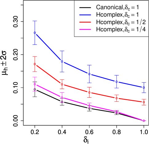
Figure 5: Mean and standard deviation of coherence as a function of indel and component sampling coverage for a $50\times 50$ indel grid and 10 Monte Carlo runs. The horizontal axis shows the indel undersampling ratio. Different colored lines correspond to the traditional measure of coherence for pure NUS (black), hypercomplex coherence for pure NUS (blue), hypercomplex coherence for a PCS approach when half of the hypercomplex components are sampled at selected indels (red) , and hypercomplex coherence for a PCS approach when a quarter of the hypercomplex components are sampled at selected indels (magenta).

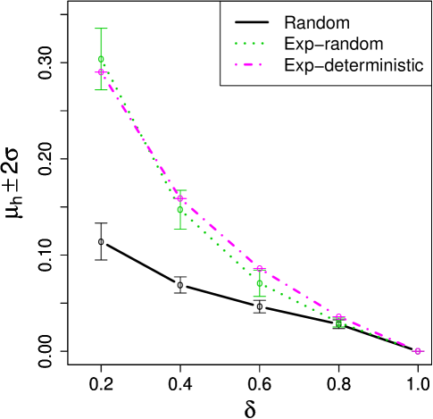
Figure 6: Hypercomplex coherence for random (solid line), exponentially-biased random (dotted line), and deterministic exponential sampling (dash-dot line) for a $50\times 50$ indel grid and 30 Monte Carlo runs. The horizontal axis shows the PCS undersampling ratio.

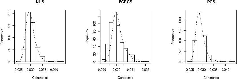
Figure 7: Histogram of hypercomplex coherence for NUS (left), FCPCS (middle), and PCS (right) for undersampling ratio $\delta=0.5$ and $100\times 100$ indel grid. The dashed curve is a fitted smooth density function.

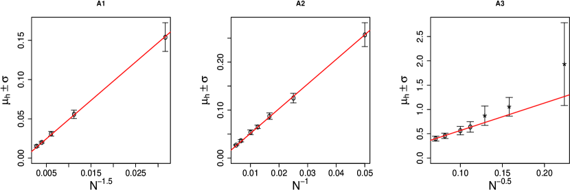
Figure 8: Hypercomplex coherence for A1 (left), A2 (middle), and A3 (right) as a function of problem size in a three dimensional RPD experiment with undersampling ratio $\delta=0.25$. The horizontal axis shows $N^{-(3-k)/2}$ where $k$ is the number of frozen dimensions for each approach. The red solid lines show the fitted lines in model (12). The fits are based on data for large enough problem sizes, i.e., $m=N^{d-k}>60$ to eliminate the second-order effects associated with very small problems sizes. Data excluded from the fits are shown with $*$ symbols.

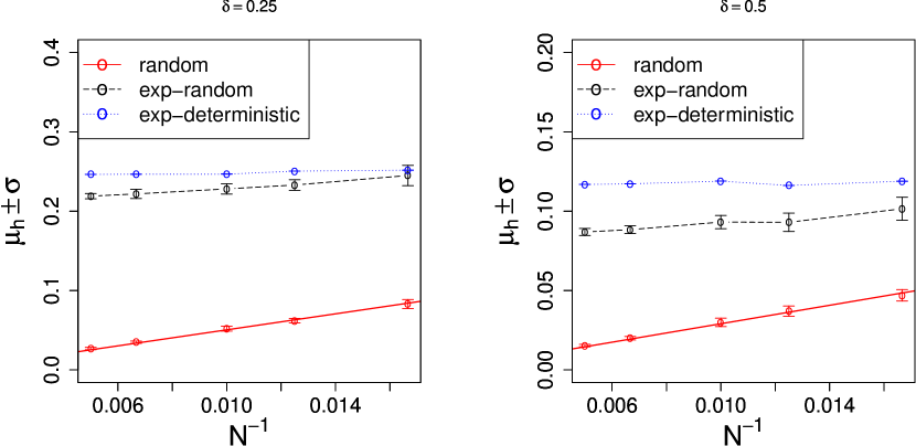
Figure 9: Hypercomplex coherence for random (red), exponentially-biased random (black), and deterministic exponential sampling (blue) as a function of problem size for undersampling ratio $\delta=0.25$ and 30 Monte Carlo runs. The horizontal axis shows $1/\sqrt{m}$ where $m=N^{2}$ is the total number of indels. The solid red line shows the fitted line according to model (14).

$\begin{array}[]{l}\includegraphics[width=361.34999pt]{figs/QQplotCoherenceDist_FOURIER_N20_delta5e-01.pdf}\\ \includegraphics[width=361.34999pt]{figs/QQplotCoherenceDist_FOURIER_N40_delta5e-01.pdf}\\ \includegraphics[width=361.34999pt]{figs/QQplotCoherenceDist_FOURIER_N80_delta5e-01.pdf}\\ \includegraphics[width=361.34999pt]{figs/QQplotCoherenceDist_FOURIER_N150_delta5e-01.pdf}\\ \includegraphics[width=361.34999pt]{figs/QQplotCoherenceDist_FOURIER_N200_delta5e-01.pdf}\\ \end{array}$

Figure 10: Quantile-quantile plot of coherence distributions: NUS versus PCS (left), NUS versus FCPCS (middle), and PCS versus FCPCS (right) for approach A2 and scheme S4 on a 2D square indel grid of size $N=20,40,80,150,200$ (top to bottom). Here, $\delta=1/2$ and $nMonte=210$. In each panel, the blue line indicates the $y=x$ identity line. If the black dots all fall along the blue line, then the two distributions are equal. If they fall below the line, then the horizontally-plotted distribution is typically larger in value than the other one.

7 Examples

We now compute and interpret the hypercomplex coherence for three-dimensional NMR problems in which two indirect dimensions are undersampled. We consider these three types of experiments:

• PCS with fixed component under-sampling ratio at all indels. In this experiment, we fix the number of hypercomplex components measured at each indel. Here $0\leq\delta_{i}\leq 1$ is the fraction of indels sampled. Similarly, $0\leq\delta_{c}\leq 1$ is the fraction of hypercomplex components sampled. We consider 8-dimensional hypercomplex numbers of the form

  $$z=\left\{c_{0}+c_{1}{\bf i}_{1}+c_{2}{\bf i}_{2}+c_{3}{\bf i}_{12}\right\}+{\bf i}_{3}\left\{c_{4}+c_{5}{\bf i}_{1}+c_{6}{\bf i}_{2}+c_{7}{\bf i}_{12}\right\}$$

  In our computations, we considered four schemes of complex reads:

  • $S1$ : $a\rightarrow\left[c_{0},c_{1}\right]$, $b\rightarrow\left[c_{2},c_{3}\right]$, $c\rightarrow\left[c_{4},c_{5}\right]$, $d\rightarrow\left[c_{6},c_{7}\right]$

  • $S2$ : $a\rightarrow\left[c_{0},c_{2}\right]$, $b\rightarrow\left[c_{1},c_{3}\right]$, $c\rightarrow\left[c_{4},c_{7}\right]$, $d\rightarrow\left[c_{5},c_{6}\right]$

  • $S3$ : $a\rightarrow\left[c_{0},c_{3}\right]$, $b\rightarrow\left[c_{1},c_{5}\right]$, $c\rightarrow\left[c_{2},c_{6}\right]$, $d\rightarrow\left[c_{4},c_{7}\right]$

  • $S4$ : $a\rightarrow\left[c_{0},c_{4}\right]$, $b\rightarrow\left[c_{1},c_{5}\right]$, $c\rightarrow\left[c_{2},c_{6}\right]$, $d\rightarrow\left[c_{3},c_{7}\right]$

  For $\delta_{c}\in\{1/4,2/4,1\}$, and $s\in\left\{S1,S2,S3,S4\right\}$, we set the following sampling rules:

  $$z_{1/4}^{s}=\left\{\begin{array}[]{ccc}a[s]&\text{if}&\chi_{1/4}=0\\ b[s]&\text{if}&\chi_{1/4}=1\\ c[s]&\text{if}&\chi_{1/4}=2\\ d[s]&\text{if}&\chi_{1/4}=3\\ \end{array}\right.$$

  $$z_{2/4}^{s}=\left\{\begin{array}[]{ccc}\left(a[s],b[s]\right)&\text{if}&\chi_{2/4}=0\\ \left(a[s],c[s]\right)&\text{if}&\chi_{2/4}=1\\ \left(a[s],d[s]\right)&\text{if}&\chi_{2/4}=2\\ \left(b[s],c[s]\right)&\text{if}&\chi_{2/4}=3\\ \left(b[s],d[s]\right)&\text{if}&\chi_{2/4}=4\\ \left(c[s],d[s]\right)&\text{if}&\chi_{2/4}=5\\ \end{array}\right.$$

  where $\chi_{\delta_{c}}$ denotes a random sample drawn from the integer set $\{0,1,\dots,(1/\delta_{c}-1)\}$ at fixed $\delta_{c}$. According to these rules and through the following approaches, we sample a subset of the hypercomplex components.

  • $\chi_{\delta_{c}}$ is drawn once for each pixel defined by $(t_{1},t_{2},t_{3})$.

  • $\chi_{\delta_{c}}$ is drawn once for each indel defined by $(t_{1},t_{2})$.

  • $\chi_{\delta_{c}}$ is drawn once for each plane defined by indirect index $t_{1}$.

  Although mathematically well-defined, these sampling approaches and schemes are not equally realistic for NMR applications, and some are only included in our analysis as instructive ‘sanity-checks’.

• Non-uniform sampling. In our NUS computtaions, all hypercomplex components are measured at the selected indels. We consider the following selection schemes:

  • Random sampling: a subset of the indels is selected by uniform random sampling.

  • Exponentially-biased sampling: indels at earlier times are more likely to be sampled than those at later times; the likelihood of sampling varies according to an exponentially-decaying probability schedule. Such sampling schemes are originally due to [15]. We implemented both a deterministic and a random exponentially-biased sampling schedule. For details, see the reproducible code distributed with this article (see section 10).

• PCS with equal sampling coverage for all components. Here, we let $\delta$ represent the sampling coverage per hypercomplex component. For each hypercomplex component, we measure $\delta$ fraction of the indels through random or exponentially-biased sampling.

7.1 Artifact patterns

We now apply the hypercomplex point spread function to study the artifacts induced by undersampling the hypercomplex Fourier transform. Figure 3 shows the hPSF for three different approaches of PCS at $\delta_{c}=1/2$, and $\delta_{i}=1$ due to a spike at $i_{0}=[0,0,0]$. We observe a certain pattern of artifacts developing due to PCS, which can be understood using lemmas 11.3 and 12.4 in the Appendix. The plots are in agreement with the belief that allowing more randomization reduces the coherence [5, 4]. In particular, restricting the randomization of PCS to the $t_{1}$ direction (i.e., A3) leads to a large nonzero point-spread along a line, while extending the randomization across two indirect dimensions $(t_{1},t_{2})$ (i.e., A2) leads to a somewhat smaller point spread throughout a plane. If we further allow randomization at every pixel (i.e., A1), the point spread is much smaller, although nonzero throughout the whole cube.

Figure 4 shows the hPSF for a spike located at a nonzero frequency, namely $i_{0}=[4,4,4]$. We observe that, in general, NUS and PCS develop different artifact patterns. However, for specific undersampling schedules, they may produce similar patterns (see top left and top middle panels). Also, we observe different patterns of artifacts for different schemes of PCS. For example, artifacts developed by scheme S4 are concentrated on positive frequency side (i.e., $i_{z}=4$) whereas scheme S2 produces smaller size artifacts spread out on both sides of the frequency domain (i.e., $i_{z}=\pm 4$). Again, these patterns can be understood using the lemmas presented in the Appendix.

7.2 Sampling coverage

Figure 5 shows the coherence averaged over 10 Monte Carlo runs as a function of sampling coverage. The black line shows the traditional measure of coherence under a pure NUS scenario. The average hypercomplex coherence, similar to the traditional coherence, decreases as the sampling coverage increases.

Figure 6 compares exponentially-biased sampling with random sampling when two indirect dimensions are involved. As expected, we observe a lower coherence for random sampling schedules.

Table 1: mean, standard error and Z-score of mean difference for NUS, FCPCS, and PCS coherence. Here, total undersampling $\delta=0.25$, nMonte = 210 and $\delta_{i}=1$ for FCPCS. The experiments are conducted for approach A2, and scheme S4 on a 2D square indel lattice of size N=40,60,80,100, and 200’. Standard errors are shown in parentheses. Numbers are rounded to the displayed precision.

	40	60	80	100	200
NUS	0.117 (6.42e-04)	0.083 (4.65e-04)	0.064 (3.23e-04)	0.052 (1.66e-04)	0.028 (1.11e-04)
PCS	0.123 (7.62e-04)	0.084 (4.47e-04)	0.064 (3.23e-04)	0.051 (1.45e-04)	0.027 (1.01e-04)
FCPCS	0.127 (6.84e-04)	0.085 (4.13e-04)	0.065 (3.08e-04)	0.053 (1.65e-04)	0.027 (9.74e-05)
Z(NUS,PCS)	-5.93	-1.63	0.73	4.18	10.26
Z(NUS,FCPCS)	-11.17	-4.18	-1.41	-3.92	6.79
Z(PCS,FCPCS)	-4.46	-2.54	-2.15	-8.36	-3.83

Table 2: mean, standard error and Z-score of mean difference for NUS, FCPCS, and PCS coherence. Here, total undersampling $\delta=0.50$, nMonte = 210 and $\delta_{i}=1$ for FCPCS. The experiments are conducted for approach A2, and scheme S4 on a 2D square indel lattice of size N=40,60,80,100, and 200’. Standard errors are shown in parentheses. Numbers are rounded to the displayed precision.

	40	60	80	100	200
NUS	0.067 (3.85e-04)	0.047 (2.23e-04)	0.037 (1.79e-04)	0.030 (9.37e-05)	0.016 (6.63e-05)
PCS	0.070 (4.04e-04)	0.048 (2.28e-04)	0.036 (1.75e-04)	0.030 (8.69e-05)	0.015 (6.44e-05)
FCPCS	0.072 (4.04e-04)	0.049 (2.75e-04)	0.037 (1.84e-04)	0.030 (8.25e-05)	0.016 (5.62e-05)
Z(NUS,PCS)	-4.71	-1.47	0.73	5.62	8.33
Z(NUS,FCPCS)	-7.96	-4.91	-2	1.43	4.99
Z(PCS,FCPCS)	-3.17	-3.55	-2.75	-4.51	-3.94

Table 3: $P$-values of the estimated intercept $\hat{\beta}_{0}$ in model (13) for RPD.

	exponent $\gamma$
approach	2	1.75	1.5	1.25	1	0.75	0.5	0.33	0.25
A1	0.021	0.020	0.050	0.010	0.010	0.009	0.009	0.009	0.010
A2	0.002	0.002	0.001	0.001	0.221	0.003	0.002	0.002	0.002
A3	0.002	0.002	0.001	0.001	0.000	0.000	0.292	0.013	0.009

Table 4: $R^{2}$ of fits in model (14) for RPD. The exponent $\gamma=(d-k)/2$ gives the best fits for all the approaches.

	exponent $\gamma$
approach	2	1.75	1.5	1.25	1	0.75	0.5	0.33	0.25
A1	0.9767	0.9916	0.9997	0.9941	0.9650	0.9028	0.8035	0.7201	0.6752
A2	0.8751	0.9122	0.9506	0.9838	0.9997	0.9801	0.9069	0.8259	0.7775
A3	0.8598	0.8923	0.9242	0.9537	0.9781	0.9946	0.9999	0.9959	0.9915

Table 5: $R^{2}$ of fits in model (14) for random PCS on 2D square indel grid and problem sizes $N=60,80,100,150,200$. The best fit occurs at $\gamma=1$.

	exponent $\gamma$
$\delta$	2	1.75	1.5	1.25	1	0.75	0.5	0.33	0.25
0.25	0.9193	0.9470	0.9714	0.9901	0.9995	0.9955	0.9741	0.9486	0.9324
0.5	0.9153	0.9440	0.9694	0.9890	0.9992	0.9959	0.9749	0.9497	0.9335

Table 6: $P$-values of the estimated intercept $\hat{\beta}_{0}$ in model (13) for random PCS on 2D square indel grid and problem sizes $N=60,80,100,150,200$.

	exponent $\gamma$
$\delta$	2	1.75	1.5	1.25	1	0.75	0.5	0.33	0.25
0.25	0.004	0.003	0.003	0.003	0.049	0.008	0.003	0.002	0.002
0.5	0.007	0.007	0.008	0.012	0.115	0.001	0.001	0.001	0.001

7.3 Comparison of NUS and PCS

Figure 7 depicts the statistical distribution of hypercomplex coherence across many random realizations of undersampling. Here NUS, FCPCS, and PCS are compared, maintaining equal number of real degrees of freedom across schemes. The three methods exhibit visually similar skewed distributions. It is very natural to test for statistical equivalence across these distributions. We begin by comparing the empirical average coherence through the following hypothesis.

Method Equivalence Hypothesis. Consider a three-dimensional NMR experiment with two indirect dimensions, each of length $N_{i}$, and a direct acquisition dimension of length $N_{a}$, leading to $N=2^{3}\cdot N_{i}^{2}N_{a}$ real coefficients. Suppose $n$ real coefficients are sampled under each of three different random sampling methods ${\cal S}_{NUS}$, ${\cal S}_{PCS}$ and ${\cal S}_{FCPCS}$ and quadrature detection in the acquisition dimension (i.e., scheme $S4$). The observed average coherence of PCS, FCPCS and NUS are the same to within sampling variation.

We consider two forms of the Method Equivalence Hypothesis. A strong form, which states the observed average coherences of NUS, PCS and FCPCS match for every $n$ and $N$, and a weak form that says the differences of the observed average coherence decays to zero with increasing $N$.

• Two-sample comparison. We consider standard statistical procedures and work with the $Z$-score of mean difference between two samples:

  $$Z(\mu_{0},\mu_{1},M_{0},M_{1})=\frac{\mu_{1}-\mu_{2}}{\hat{SD}(\mu_{0}-\mu_{1},M_{0},M_{1})}$$

  Here $\mu_{i}$ denotes “the observed average hypercomplex coherence for method $i$” and $\hat{SD}(\mu_{1}-\mu_{2},M_{1},M_{2})$ is the appropriate standard error of comparing means for possibly unequal sample sizes $M_{i}$. We can now state the strong null hypothesis in terms of Z-scores:

  • Strong Null Hypothesis. The $Z$-scores of the mean differences are small for all $N$.

• Asymptotic Equivalence. It is not implausible to see significant differences in average coherence value at small $N$, and so the strict from of equivalence seems implausible a priori. Can we hope that the difference in average coherence becomes insignificant with increasing $N$? To investigate this possibility, we consider:

  • Weak Null Hypothesis. The $Z$-scores of the mean differences decrease with increasing $N$.

• Rejection of Method Equivalence Hypothesis. Our results for testing the Method Equivalence Hypothesis are summarized in Tables 1 and 2 for undersmapling ratios $\delta=0.25$, and $\delta=0.5$. The $Z$-scores do not support the weak or strong form of the Method Equivalence Hypothesis although the difference of the average coherences between the methods seem to be inconspicuous.

• Q-Q plots. To further understand the relation between different sampling methods, we present quantile-quantile plots as shown in Figure 10. Though the deviation from the identity line is small ($\sim<5\%$), we do see that PCS gives slightly smaller coherence for larger problem sizes ($N>80$) whereas NUS performs slightly better for smaller problem sizes ($N<80$). At $N=80$, we observe no significant difference. Moreover, we see that PCS always outperforms FCPCS by giving lower coherence. Though there is a subtle statistically observable difference between these methods, we must point out that from a practical point of view these differences seem unimportant (see Table 2 for a comparison).

7.4 Comparison of different schemes

We have introduced four different schemes $S1$ to $S4$ for partial component sampling. These schemes, though mathematically well-defined, are not equally realistic for the setup of NMR experiments in which quadrature detection is employed. Actually, only scheme $S4$ is realistic for quadrature detection because both $sine$ and $cosine$ components of the acquisition dimension (i.e., $t_{d}$) are sampled together. This is why we chose to work with this scheme in the Method Equivalence Hypothesis.

It is mathematically instructive to test whether these schemes yield different coherence values if all other experimental parameters are kept intact. We therefore test the following hypothesis.

Scheme Equivalence Hypothesis. Consider a three-dimensional NMR experiment with two indirect dimension each of length $N_{i}$, and acquisition dimensions of length $N_{a}$ leading to $N=2^{3}\cdot N_{i}^{2}N_{a}$ real coefficients. Suppose $n$ coefficients are sampled through four different schemes $S1$, $S2$, $S3$, and $S4$ and approach $A2$ (i.e., sampled component subset changes from indel to indel). The average hypercomplex coherence for all these four schemes are equal.

Similar to the Method Equivalence Hypothesis, we consider the Z-score as a statistical measure of significance, and examine the strict and weak forms of Scheme Equivalence Hypothesis. Our results, shown in Table LABEL:SchemeEquivalence, reject both forms of the Scheme Equivalence hypothesis.

7.5 Finite-N scaling

Consider an RPD experiment with $d$ dimensions each of length $N$. Further, suppose we freeze $k<d$ dimensions so that randomization of selected component subset is employed in only $d-k$ dimensions. For example in approach A3, $d=3$ and $k=2$. For large enough problem sizes, we propose the following finite-$N$ scaling model.

$$\mu(N)=\beta_{1}N^{-(d-k)/2}.$$ (12)

Here $\mu$ is the expected value of hypercomplex coherence. Figure 8 shows the data and fitted lines for the three approaches A1,A2, and A3.

7.5.1 Justification of exponent.

To justify the scaling law suggested in model (12), we consider a three-dimensional RPD experiment in which 2 out of 8 components are sampled according to three different approaches A1, A2, and A3. We examine the two following fitting models:

$$\beta(N)=\beta_{0}+\beta_{1}(\gamma)N^{-\gamma}+error$$ (13)

and

$$\beta(N)=\beta_{1}(\gamma)N^{-\gamma}+error.$$ (14)

The first model includes an intercept term allowing us to assess the possible significance of coefficient $\beta_{0}$. We examine the goodness of fit for three approaches of RPD as the exponent $\gamma$ varies.

The $P$-values associated with coefficient $\beta_{0}$ of model (13) are reported in Table 3. The fitting exercise shows that $\gamma=(d-k)/2$ is the only exponent to make the case of $\beta_{0}\neq 0$ very weak for all the approaches.

Table 4 shows $R^{2}$ of fits in model (14). Evidently $\gamma=(d-k)/2$ gives the best fits for all the approaches.

7.5.2 PCS finite-N scaling.

So far we have shown that coherence of RPD as a function of problem size $N$ follows the scaling law given by model (12). Can we hope that the same model applies to random PCS with equal sampling coverage for all components?

We consider a three-dimensional NMR problem with two indirect dimensions and randomize the PCS schedule across the entire $N^{2}$ indels. Figure 9 shows the data of random PCS together with the fitted line in model (14). For comparison purposes, we show the data corresponding to exponentially-biased random and deterministic exponential sampling on the sample plot. Evidently, the random case has lower coherence and decays faster with increasing problem size compared to the other two.

Table 5 shows $R^{2}$ of fits for the random case at two different undersampling ratios $\delta\in\{1/4,1/2\}$. Similar to the RPD case for approach A2, we see that the best fit occurs at $\gamma=1$, verifying the adequacy of model 12 for general random PCS schedules. Finally, Table 6 shows the $P$-values associated with coefficient $\beta_{0}$ of model (13) for random PCS. Evidently, $\gamma=1$ makes the evidence for $\beta_{0}\neq 0$ the weakest.

8 Discussion

It has been shown that more randomization in a NUS schedule results in lower coherence [4]. We showed this to be equally true for hypercomplex-aware undersampling, in which a subset of all components are sampled. Our results show that coherence is the smallest when randomization of partial-component sampling is employed in as many indirect dimensions as possible.

Unlike [13], the results of this article do not suggest a synergistic effect of PCS in reducing the sampling coherence compared to NUS; For a given fixed number of degrees of freedom for sampling, one observes almost the same coherence value no matter which way of expending the degrees of freedom is used. This seemingly contradictory observation is perhaps due to a different notion of coherence used in [13].

9 Concluding remarks

We presented a definition of coherence appropriate for the hypercomplex-valued setting of multi-dimensional NMR. Though the hypercomplex coherence is general, in the sense that it can be applied to all undersampling classes, we would like to point out that this measure is inherently different from the canonical notion of coherence for $d\geq 2$ even for the case of full-component random sampling in which one samples uniformly at random from the collection of all indels, or even of all pixels. This difference comes from the fact that in general $\sigma_{max}(\Phi(z))\neq|z|_{H}$ for $z\in\mathbb{H}_{d}$.

10 Reproducible Research

The code and data that generated the figures in this article may be found online at http://purl.stanford.edu/xn744fp3001[16].

References

Appendix

Definition 11 (uniformly-sampled dimension).

Consider a $d$-dimensional sampling set ${\cal T}$, sampled from within a Cartesian grid of $T_{1}\times T_{2},\dots,T_{d}$ equispaced points. We say that dimension $i\in\{1,2,\dots,d\}$ is uniformly sampled if for each $(d-1)$-tuple $t^{(i)}=(t_{j}:j\neq i)$ arising from a sample $t\in{\cal T}$, every $d$-tuple $t^{(i)}(k)=(t_{1},\dots,t_{i-1},k,t_{i+1},\dots,t_{d}),\ k=1,\dots,N_{i}$, occurs as a sample $t\in{\cal T}$.

Lemma 11.3 (NUS cross-correlation).

Suppose that in the sampling set ${\cal T}\in Z_{T_{1}}\times\dots\times Z_{T_{d}}$, the dimension indecis $u\in U$ are all sampled uniformly and sampling is full-component. Let $F_{k}(t)\in\mathbb{H}_{d}$ denote the $(t,k)$ coefficient of the hypercomplex Fourier matrix for $t=(t_{1},\dots,t_{d})$, and $k=(k_{1},\dots,k_{d})$,

$$F_{k}(t)=\frac{1}{\sqrt{\prod_{j}T_{j}}}\exp{(\sum_{j=1}^{d}2\pi{\bf i}_{j}k_{j}t_{j}/T_{j})},$$

and $\rho_{k,\ell}\in\mathbb{H}_{d}$ denote the cross-correlation between two distinct columns $k$, and $\ell$,

$$\rho_{k,\ell}=\sum_{t\in{\cal T}}F_{k}(t)F_{\ell}^{\sharp}(t).$$

Then, $\rho_{k,\ell}=0$ unless $k_{u}=\ell_{u}\text{\ \ for all \ \ }u\in U$

Proof.

The $(t,k)$ element of the hypercomplex Fourier matrix is

$$F_{k}(t)=\frac{1}{\sqrt{\prod_{j}T_{j}}}\exp{(\sum_{j=1}^{d}2\pi{\bf i}_{j}k_{j}t_{j}/T_{j})}$$

where $t=(t_{1},\dots,t_{d})$, and $k=(k_{1},\dots,k_{d})$.

Let ${\cal T}$ denote the set of all tuples $t=(t_{1},\dots,t_{d})$ that get sampled. Let $D=\{1,2,\dots,d\}$ represent the set of all dimensions. Further, let $U$ denote dimensions that are sampled uniformly and exhaustively and $D\backslash U$ the rest that are sampled nonuniformly. For each index $j\in U$, let ${\cal T}_{j}=\{0,\dots,T_{j}-1\}$ denote the full range of that index. Let ${\cal T}_{D\backslash U}$ denote the collection of all sampled indices in the non-uniformly-sampled variables only. Then

$${\cal T}={\cal T}_{D\backslash U}\times\prod_{j\in U}{\cal T}_{j}.$$

In the case of full-component sampling (i.e., NUS), the cross-correlation between two distinct columns $k$, and $\ell$ is given by,

$$\rho_{k,\ell} = \sum_{t\in{\cal T}}F_{k}(t)F_{\ell}^{\sharp}(t)$$

$$= \left(\frac{1}{\prod_{j\in D\backslash U}T_{j}}\sum_{t\in{\cal T}_{D\backslash U}}\exp{(\sum_{j\in D\backslash U}2\pi{\bf i}_{j}t_{j}(k_{j}-\ell_{j})/T_{j})}\right)\dots$$

$$\left(\prod_{j\in U}\frac{1}{T_{j}}\sum_{t_{j}\in{\cal T}_{j}}\exp{(2\pi{\bf i}_{j}t_{j}(k_{j}-\ell_{j})/T_{j})}\right)$$

$$= \left(\frac{1}{\prod_{j\in D\backslash U}T_{j}}\sum_{t\in{\cal T}_{D\backslash U}}\exp{(\sum_{j\in D\backslash U}2\pi{\bf i}_{j}t_{j}(k_{j}-\ell_{j})/T_{j})}\right)\cdot\prod_{j\in U}\delta(k_{j}-\ell_{j})$$

for uniformly sampled direction $u\in U$.

Here we used the exponential sum (6) in each uniformly-sampled coordinate, as well as the commutativity of the hypercomplex algebra, and $\delta(\cdot)$ denotes the Kronecker symbol. We see that $\rho_{k,\ell}=0$ unless $k_{u}=\ell_{u}\text{\ \ for all \ \ }u\in U$. ∎

So far we have shown that under full-component sampling, if certain coordinates are sampled uniformly, then the cross-correlation between two distinct columns $k=(k_{1},\dots,k_{d})$ and $\ell=(\ell_{1},\dots,\ell_{d})$ of hypercomplex fourier matrix vanishes unless all their corresponding indecis of the uniformly-sampled coordinates match. When the cross-correlation does not vanish, one obtains a hypercomplex number $\rho_{k,\ell}$, which can be viewed as a $2^{d}$ by $2^{d}$ matrix $\Sigma_{k,\ell}=\Phi({\rho}_{k,\ell})$ where $\Phi$ is the matrix isomorphism defined for hypercomplex algebra in this article.

To generalize the results to partial-component sampling, we need to further examine the isomorphic matrix associated with correlation $\rho_{k,\ell}$ in detail. Before we proceed, it is helpful to define the quadrature acquisition in PCS.

Definition 12 (quadrature acquisition).

Let $F_{k}(t)\in\mathbb{H}_{d}$ denote the $(t,k)$ coefficient of the hypercomplex Fourier matrix at $t=(t_{1},\dots,t_{d})$ and $k=(k_{1},\dots,k_{d})$,

$$F_{k}(t)=\frac{1}{\sqrt{\prod_{j}T_{j}}}\exp{(\sum_{j=1}^{d}2\pi{\bf i}_{j}k_{j}t_{j}/T_{j})}.$$

Each coefficient generates $2^{d}$ components given by,

$$z_{g}=\frac{1}{\sqrt{\prod_{j=1}^{d}T_{j}}}\beta_{1}\times\dots\times\beta_{d}$$

where

$$\beta_{j}=\left\{\begin{array}[]{cc}\cos(2\pi k_{j}t_{j}/T_{j})&j\not\in g\\ \sin(2\pi k_{j}t_{j}/T_{j})&j\in g\end{array}\right.$$

We say ‘quadrature acquisition’ is employed in dimension $i$ if for each $(d-1)$-tuple $(\beta_{j}:j\neq i)$ arising from a sampling schedule of components ${\cal J}$, both components

$$\frac{1}{\sqrt{\prod_{j=1}^{d}T_{j}}}\left(\prod_{j\neq i}\beta_{j}\right)\cos(2\pi k_{i}t_{i}/T_{i}),\quad\frac{1}{\sqrt{\prod_{j=1}^{d}T_{j}}}\left(\prod_{j\neq i}\beta_{j}\right)\sin(2\pi k_{i}t_{i}/T_{i})$$

occur in ${\cal J}$.

Consider the end-to-end partial component sampling matrix denoted by $A$. Let us represent the entry of this matrix corresponding to frequency $k=(k_{1},\dots,k_{d})$ and sampled time $t=(t_{1},\dots,t_{d})\in{\cal T}$ by

$$a_{rc}^{k}(t),\quad r\in J(t),\ \ c=1,\dots,2^{d}$$

where $J(t)\subset\{1,\dots,2^{d}\}$ is a set that contains the indecis of selected components at time $t$. It is easily verified that the entries of such sampling matrix takes the values

$$a_{rc}^{k}(t)=\frac{\alpha^{rc}}{\sqrt{\prod_{j}T_{j}}}\beta_{1}^{rc}\times\dots\times\beta_{d}^{rc}$$

for appropriate values of $\beta_{j}^{rc}\in\left\{\cos(2\pi k_{j}t_{j}/T_{j}),\sin(2\pi k_{j}t_{j}/T_{j}\right\}$ and $\alpha^{rc}\in\{-1,1\}$. The $2^{d}\times 2^{d}$ cross-correlation matrix between two distinct columns $k$, and $\ell$ is then given by

$$\Sigma_{u,v}^{k,\ell}=\sum_{t\in{\cal T}}\sum_{r\in J(t)}a_{ru}^{k}(t)a_{rv}^{\ell}(t),\quad(u,v)\in\{1,\dots,2^{d}\}^{2}.$$

To clarify, let us consider three different PCS scenarios in a two-dimensional NMR experiment in which one of the dimensions (direct dimension) is sampled uniformly. Namely,

• (NUS): $J(t)=\{1,2,3,4\},\quad t_{1}\in{\cal T}_{1},\ t_{2}\in\{1,\dots,2^{d}\}$.

  $$a_{\{1:4,1:4\}}^{k}(t)=\frac{1}{\sqrt{T_{1}T_{2}}}\left(\begin{array}[]{cccc}C_{2}C_{1}&-C_{2}S_{1}&-S_{2}C_{1}&S_{2}S_{1}\\ C_{2}S_{1}&C_{2}C_{1}&-S_{2}S_{1}&-S_{2}C_{1}\\ S_{2}C_{1}&-S_{2}S_{1}&C_{2}C_{1}&-C_{2}S_{1}\\ S_{2}S_{1}&-S_{2}C_{1}&C_{2}S_{1}&C_{2}C_{1}\\ \end{array}\right)$$

• (Quadrature PCS): $J(t)=\{1,3\},\quad t_{1}\in{\cal T}_{1},\ t_{2}\in\{1,\dots,2^{d}\}$

  $$a_{\{1:2,1:4\}}^{k}(t)=\frac{1}{\sqrt{T_{1}T_{2}}}\left(\begin{array}[]{cccc}C_{2}C_{1}&-C_{2}S_{1}&-S_{2}C_{1}&S_{2}S_{1}\\ S_{2}C_{1}&-S_{2}S_{1}&C_{2}C_{1}&-C_{2}S_{1}\\ \end{array}\right)$$

• (Non-quadrature PCS): $J(t)=\{1\},\quad t_{1}\in{\cal T}_{1},\ t_{2}\in\{1,\dots,2^{d}\}$

  $$a_{\{1,1:4\}}^{k}(t)=\frac{1}{\sqrt{T_{1}T_{2}}}\left(\begin{array}[]{cccc}C_{2}C_{1}&-C_{2}S_{1}&-S_{2}C_{1}&S_{2}S_{1}\\ \end{array}\right)$$

In these examples $C_{j}=\cos(2\pi k_{j}t_{j}/T_{j})$ and $S_{j}=\sin(2\pi k_{j}t_{j}/T_{j})$ for $j=1,2$.

For (NUS) (i.e., full-component sampling), one can write

$$\Sigma_{1,2}^{k,\ell} = \sum_{t\in{\cal T}}\sum_{r=1}^{4}a_{r1}^{k}(t)a_{r2}^{\ell}(t)$$

$$= \sum_{t\in{\cal T}}(C_{2}C_{1})^{k}(-C_{2}S_{1})^{\ell}+(C_{2}S_{1})^{k}(C_{2}C_{1})^{\ell}+(S_{2}C_{1})^{k}(-S_{2}S_{1})^{\ell}+(S_{2}S_{1})^{k}(-S_{2}C_{1})^{\ell}$$

$$= \sum_{t\in{\cal T}}-C_{1}^{k}S_{1}^{\ell}\left(C_{2}^{k}C_{2}^{\ell}+S_{2}^{k}S_{2}^{\ell}\right)+S_{1}^{k}C_{1}^{\ell}\left(C_{2}^{k}C_{2}^{\ell}+S_{2}^{k}S_{2}^{\ell}\right)$$

$$= \sum_{t\in{\cal T}}\left(S_{1}^{k}C_{1}^{\ell}-C_{1}^{k}S_{1}^{\ell}\right)\left(C_{2}^{k}C_{2}^{\ell}+S_{2}^{k}S_{2}^{\ell}\right)$$

$$= \sum_{t_{1}\in{\cal T}_{1}}\left(S_{1}^{k}C_{1}^{\ell}-C_{1}^{k}S_{1}^{\ell}\right)\sum_{t_{2}\in{\cal T}_{2}}\left(C_{2}^{k}C_{2}^{\ell}+S_{2}^{k}S_{2}^{\ell}\right)$$

$$= \sum_{t_{1}\in{\cal T}_{1}}\sin(2\pi(k_{1}-\ell_{1})t_{1}/T_{1})\sum_{t_{2}\in{\cal T}_{2}}\cos(2\pi(k_{2}-\ell_{2})t_{2}/T_{2}).$$

If one continues computing the other entries of cross-correlation matrix $\Sigma^{k,l}$, one sees that all non-trivial entries contain either $\sum_{t_{j}\in{\cal T}_{j}}\sin\left(2\pi t_{j}(k_{j}-\ell_{j})/T_{j}\right)$ or $\sum_{t_{j}\in{\cal T}_{j}}\cos\left(2\pi t_{j}(k_{j}-\ell_{j})/T_{j}\right)\text{\ \ for all \ }j\in D$. Therefore, $\Sigma^{k,\ell}=0$ unless $k_{u}=\ell_{u}\text{\ \ for all uniformly sampled coordinate \ \ }u\in U$ and so we recover Lemma (11.3) as expected.

For (quadrature PCS) case, we can write

$$\Sigma_{1,2}^{k,\ell} = \sum_{t\in{\cal T}}\sum_{r=1,3}a_{r1}^{k}(t)a_{r2}^{\ell}(t)$$

$$= \sum_{t\in{\cal T}}(C_{2}C_{1})^{k}(-C_{2}S_{1})^{\ell}+(S_{2}C_{1})^{k}(-S_{2}S_{1})^{\ell}$$

$$= \sum_{t\in{\cal T}}-C_{1}^{k}S_{1}^{\ell}\left(C_{2}^{k}C_{2}^{\ell}+S_{2}^{k}S_{2}^{\ell}\right)$$

$$= \sum_{t_{1}\in{\cal T}_{1}}\cos\left(2\pi t_{1}k_{1}/T_{1}\right)\sin\left(2\pi t_{1}\ell_{1}/T_{1}\right)\sum_{t_{2}\in{\cal T}_{2}}\cos(2\pi(k_{2}-\ell_{2})t_{2}/T_{2}).$$

Computing other non-trivial entries of the cross-correlation matrix in this case, one observes that they contain either $\sum_{t_{j}\in{\cal T}_{j}}\sin\left(2\pi t_{j}(k_{j}-\ell_{j})/T_{j}\right)$ or $\sum_{t_{j}\in{\cal T}_{j}}\cos\left(2\pi t_{j}(k_{j}-\ell_{j})/T_{j}\right)\text{\ \ for each quadrature acquisition dimensions \ }j\in Q$ (In the example above $Q={2}$). If, further, all the uniformly-sampled dimensions are acquired by quadrature detection (i.e., $U=Q$), we see that $\Sigma^{k,\ell}=0$ unless $k_{j}=\ell_{j}\text{\ \ for all uniformly sampled coordinate \ \ }j\in U$ which can be considered as a generalization of Lemma (11.3).

For the third scenario (non-quadrature PCS), we have

$$\Sigma_{1,2}^{k,\ell} = \sum_{t\in{\cal T}}\sum_{r=1}a_{r1}^{k}(t)a_{r2}^{\ell}(t)$$

$$= \sum_{t\in{\cal T}}(C_{2}C_{1})^{k}(-C_{2}S_{1})^{\ell}$$

$$= \sum_{t\in{\cal T}}-(C_{1}^{k}S_{1}^{\ell})\left(C_{2}^{k}C_{2}^{\ell}\right)$$

$$= \sum_{t_{1}\in{\cal T}_{1}}\cos\left(2\pi t_{1}k_{1}/T_{1}\right)\sin\left(2\pi t_{1}\ell_{1}/T_{1}\right)\sum_{t_{2}\in{\cal T}_{2}}\cos(2\pi k_{2}t_{2}/T_{2})\cos(2\pi\ell_{2}t_{2}/T_{2})$$

Evidently, under non-quadrature PCS the factors do not necessarily contain $\sum_{t_{j}\in{\cal T}_{j}}\sin\left(2\pi t_{j}(k_{j}-\ell_{j})/T_{j}\right)$ or $\sum_{t_{j}\in{\cal T}_{j}}\cos\left(2\pi t_{j}(k_{j}-\ell_{j})/T_{j}\right)$. Instead, the non-trivial entries of $\Sigma^{k,\ell}$ may contain the following

$$\sum_{t_{j}\in{\cal T}_{j}}\cos\left(2\pi t_{j}k_{j}/T_{j}\right)\cos\left(2\pi t_{j}\ell_{j}/T_{j}\right) = \sum_{t_{j}\in{\cal T}_{j}}\frac{1}{2}\left[\cos\left(2\pi t_{j}(k_{j}-\ell_{j})/T_{j}\right)+\cos\left(2\pi t_{j}(k_{j}+\ell_{j})/T_{j}\right)\right]$$

$$\sum_{t_{j}\in{\cal T}_{j}}\sin\left(2\pi t_{j}k_{j}/T_{j}\right)\sin\left(2\pi t_{j}\ell_{j}/T_{j}\right) = \sum_{t_{j}\in{\cal T}_{j}}\frac{1}{2}\left[\cos\left(2\pi t_{j}(k_{j}-\ell_{j})/T_{j}\right)-\cos\left(2\pi t_{j}(k_{j}+\ell_{j})/T_{j}\right)\right]$$

$$\sum_{t_{j}\in{\cal T}_{j}}\sin\left(2\pi t_{j}k_{j}/T_{j}\right)\cos\left(2\pi t_{j}\ell_{j}/T_{j}\right) = \sum_{t_{j}\in{\cal T}_{j}}\frac{1}{2}\left[\sin\left(2\pi t_{j}(k_{j}+\ell_{j})/T_{j}\right)+\sin\left(2\pi t_{j}(k_{j}-\ell_{j})/T_{j}\right)\right]$$ (15)

Therefore, under non-quadrature partial component sampling $\Sigma^{k,\ell}=0$ unless $k_{u}=\ell_{u}\text{\ \ or \ \ }k_{u}=T_{u}-\ell_{u}\text{\ \ for all \ \ }u\in U$ due to the exponential sum (6) . We are now ready to establish the following lemma.

Lemma 12.4 (PCS cross-correlation).

Suppose that in the sampling set ${\cal T}\in Z_{T_{1}}\times\dots\times Z_{T_{d}}$, the dimension $u\in U$ are all sampled uniformly and sampling is partial-component. Let $D=\{1,\dots,2^{d}\}$ be the set of all dimensions and $Q\subset D$ represent all dimensions in which quadrature acquisition is employed. Further, let $A\in R^{n\times N2^{d}}$ denote the end-to-end partial component sampling matrix with entries corresponding to frequency $k=(k_{1},\dots,k_{d})$, and sampled time $t=(t_{1},\dots,t_{d})\in{\cal T}$ given by

$$a_{rc}^{k}(t),\quad r\in J(t_{D\backslash U}),\ \ c=1,\dots,2^{d}.$$

where $J(t_{D\backslash U})\subset D$ is a set that contains the indecis of selected components corresponding to tuple $\left(t_{j},\ j\not\in U\right)$. Further, let $\Sigma^{k,\ell}\in R^{2^{d}\times 2^{d}}$ denote the cross-correlation between two distinct columns $k$, and $\ell$

$$\Sigma_{u,v}^{k,\ell}=\sum_{t\in{\cal T}}\sum_{r\in J(t)}a_{ru}^{k}(t)a_{rv}^{\ell}(t),\quad(u,v)\in D\times D.$$

Then, $\Sigma^{k,\ell}=0$ unless

$$k_{u}=\left\{\begin{array}[]{ll}\ell_{u}&u\in U\text{ \ and \ }u\in Q\\ \ell_{u}\text{ \ or \ }(T_{u}-\ell_{u})&u\in U\text{ \ and \ }u\not\in Q\end{array}\right..$$

Proof.

The hypercomplex Fourier matrix is given by

$$F(t,k)=\otimes_{j=1}^{d}\left(\begin{array}[]{cc}\cos(2\pi k_{j}t_{j}/T_{j})&-\sin(2\pi k_{j}t_{j}/T_{j})\\ \sin(2\pi k_{j}t_{j}/T_{j})&\cos(2\pi k_{j}t_{j}/T_{j})\end{array}\right).$$

The end-to-end sampling matrix is a partially sampled hypercomplex Fourier matrix whose entries are given by

$$a_{rc}^{k}(t)=\frac{\alpha^{rc}}{\sqrt{\prod_{j}T_{j}}}\beta_{1}^{rc}\times\dots\times\beta_{d}^{rc},\quad r\in J(t_{D\backslash U}),\ \ c=1,\dots,2^{d},$$

for appropriate values of $\alpha^{rc}\in\{-1,1\}$ and $\beta_{j}^{rc}\in\left\{\cos(2\pi k_{j}t_{j}/T_{j}),\sin(2\pi k_{j}t_{j}/T_{j}\right\}\text{\ for all \ }j\in D$. Then, the cross-correlation between two distinct columns $k$, and $\ell$ is

$$|\Sigma_{u,v}^{k,\ell}| = \left|\sum_{t\in{\cal T}}\sum_{r\in J(t_{D\backslash U})}a_{ru}^{k}(t)a_{rv}^{\ell}(t)\right|$$

$$= \left|\frac{1}{\prod_{j=1}^{d}T_{j}}\sum_{t\in{\cal T}}\sum_{r\in J(t_{D\backslash U})}\left(\alpha^{ru}\prod_{j=1}^{d}\beta_{j}^{ru}\right)_{k}\left(\alpha^{rv}\prod_{j=1}^{d}\beta_{j}^{rv}\right)_{\ell}\right|$$

$$= \left|\frac{1}{\prod_{j=1}^{d}T_{j}}\sum_{r\in J(t_{D\backslash U})}(\alpha^{ru}\alpha^{rv})\sum_{t\in{\cal T}}\prod_{j=1}^{d}(\beta_{j}^{ru})_{k}(\beta_{j}^{rv})_{\ell}\right|$$

$$= \left|\sum_{r\in J(t_{D\backslash U})}(\alpha^{ru}\alpha^{rv})\left\{\left(\frac{1}{\prod_{j\in U\&j\in Q}T_{j}}\sum_{t_{j}\in T_{j}}\prod_{j\in U\&j\in Q}(\beta_{j}^{ru})_{k}(\beta_{j}^{rv})_{\ell}\right)\right.\right.\dots$$

$$\left(\frac{1}{\prod_{j\in U\&j\not\in Q}T_{j}}\sum_{t_{j}\in T_{j}}\prod_{j\in U\&j\not\in Q}(\beta_{j}^{ru})_{k}(\beta_{j}^{rv})_{\ell}\right)\dots$$

$$\left.\left.\left(\frac{1}{\prod_{j\in D\backslash U}T_{j}}\sum_{t_{j}\in{\cal T}_{D\backslash U}}\prod_{j\in D\backslash U}(\beta_{j}^{ru})_{k}(\beta_{j}^{rv})_{\ell}\right)\right\}\right|$$

$$= (\frac{1}{2})^{\{\#j:j\in Q\&j\in U\}}\prod_{j\in U\&j\in Q}\delta(k_{j}-l_{j})\prod_{j\in U\&j\not\in Q}\frac{1}{2}\left\{\delta(k_{j}-l_{j})\pm\delta(k_{j}+l_{j})\right\}\dots$$

$$\frac{1}{\prod_{j\in D\backslash U}T_{j}}\left|\sum_{r\in J(t_{D\backslash U})}(\alpha^{ru}\alpha^{rv})\left\{\sum_{t_{j}\in{\cal T}_{D\backslash U}}\prod_{j\in D\backslash U}(\beta_{j}^{ru})_{k}(\beta_{j}^{rv})_{\ell}\right\}\right|$$

where we used trigonometric identities (Appendix) and the exponential sum (6) in the uniformly sampled coordinates together with commutativity of the hypercomplex algebra. In the ‘quadrature acquisition’ dimensions, we expect to recover factors $\exp(2\pi k_{j}t_{j}/T_{j}),j\in Q$. We observe that $\Sigma_{u},v^{k,\ell}=0$ unless

$$k_{u}=\left\{\begin{array}[]{ll}\ell_{u}&u\in U\text{ \ and \ }u\in Q\\ \ell_{u}\text{ \ or \ }(T_{u}-\ell_{u})&u\in U\text{ \ and \ }u\not\in Q\end{array}\right.$$

∎

Under exhaustive sampling, all coordinates are acquired by quadrature acquisition and we recover Lemma 11.3.

References

• [1] M. W. Maciejewski, M. Fenwick, A. D. Schuyler, A. S. Stern, V. Gorbatyuk, J. C. Hoch, Random phase detection in multidimensional NMR, PNAS 108 (40) (2011) 16640–4.
• [2] A. D. Schuyler, M. W. Maciejewski, A. S. Stern, J. C. Hoch, Formalism for hypercomplex multidimensional NMR employing partial component subsampling, Journal of Magnetic Resonance 227 (2013) 20–24.
• [3] J. C. J. Barna, E. D. Laue, M. R. Mayger, J. Skilling, S. J. P. Worrall, Reconstruction of phase-sensitive two-dimensional nuclear-magnetic resonance spectra using maximum entropy, Biochemical Society Transactions 14 (1986) 1262–1263.
• [4] J. C. Hoch, M. W. Maciejewski, M. Mobli, A. D. Schuyler, A. S. Stern, Nonuniform sampling and maximum entropy reconstruction in multidimensional NMR, Accounts of Chemical Research 47 (2) (2013) 708–717.
• [5] M. Lustig, D. L. Donoho, J. M. Santos, J. M. Pauly, Compressed sensing MRI, IEEE Signal Processing Magazine 72.
• [6] D. L. Donoho, X. Huo, Uncertainty principles and ideal atomic decomposition, IEEE Trans. Inform. Theory 47 (7) (2001) 2845–2862.
• [7] D. L. Donoho, M. Elad, Optimally sparse representation in general (nonorthogonal) dictionaries via $\ell_{1}$ minimization, PNAS 100 (5) (2002) 2197–2202.
• [8] J. A. Tropp, Greed is Good: Algorithmic results for sparse approximation, IEEE Trans. Inform. Theory 50 (10) (2004) 2231–2242.
• [9] D. J. States, R. A. Haberkorn, D. J. Ruben, A two-dimensional nuclear overhauser experiment with pure absorption phase in four quadrants, Journal of Magnetic Resonance 48 (2) (1982) 286–292.
• [10] M. A. Delsuc, Spectral representation of 2D NMR spectra by hypercomplex numbers, Journal of Magnetic Resonance 77 (1) (1988) 22–35.
• [11] G. Bodenhausen, R. R. Ernst, The accordion experiment, a simple approach to three-dimensional NMR spectroscopy, Journal of Magnetic Resonance 45 (1981) 367?373.
• [12] J. C. Hoch, A. S. Stern, NMR Data Processing, 1st Edition, Wiley-Liss, Inc., 605 Third Avenue, New York, NY, 10158-0012, USA, 1996.
• [13] A. D. Schuyler, M. W. Maciejewski, A. S. Stern, J. C. Hoch, Nonuniform sampling of hypercomplex multidimensional NMR experiments: Dimensionality, quadrature phase and randomization., Journal of Magnetic Resonance 254 (2015) 121–130.
• [14] A. Abian, Linear Associative Algebras, Pergamon Press Inc., Maxwell house, Fairview park, Elmsford, N.Y. 10523, 1971.
• [15] J. C. J. Barna, E. D. Laue, M. R. Mayger, J. Skilling, S. J. P. Worrall, Exponential sampling, an alternative method for sampling in two-dimensional NMR experiments, Journal of Magnetic Resonance 73 (1987) 69–77.
• [16] H. Monajemi, D. L. Donoho, J. Hoch, A. Schuyler, Code and data supplement to ”Incoherence of partial-component sampling in multidimensional NMR”, Stanford Digital Repository, Available at:http://purl.stanford.edu/xn744fp3001 (2016).