A Digital Hardware Fast Algorithm and FPGA-based Prototype for a Novel 16-point Approximate DCT for Image Compression Applications

The discrete cosine transform (DCT) is the key step in many image and video coding standards. The 8-point DCT is an important special case, possessing several low-complexity approximations widely investigated. However, 16-point DCT transform has energy compaction advantages. In this sense, this paper presents a new 16-point DCT approximation with null multiplicative complexity. The proposed transform matrix is orthogonal and contains only zeros and ones. The proposed transform outperforms the well-know Walsh-Hadamard transform and the current state-of-the-art 16-point approximation. A fast algorithm for the proposed transform is also introduced. This fast algorithm is experimentally validated using hardware implementations that are physically realized and verified on a 40 nm CMOS Xilinx Virtex-6 XC6VLX240T FPGA chip for a maximum clock rate of 342 MHz. Rapid prototypes on FPGA for 8-bit input word size shows significant improvement in compressed image quality by up to 1-2 dB at the cost of only eight adders compared to the state-of-art 16-point DCT approximation algorithm in the literature [S. Bouguezel, M. O. Ahmad, and M. N. S. Swamy. A novel transform for image compression. In Proceedings of the 53rd IEEE International Midwest Symposium on Circuits and Systems (MWSCAS), 2010].

Keywords
DCT Approximation, Fast algorithms, FPGA

1 Introduction

The discrete cosine transform (DCT) [1, 38, 12] is a pivotal tool in digital signal processing, whose popularity is mainly due to its good energy compaction properties. In fact, the DCT is a robust approximation for the optimal Karhunen-Loève transform when first-order Markov signals, such as images, are considered [38, 12, 30]. Indeed, the DCT has found application in several image and video coding schemes [5, 12], such as JPEG [36], MPEG-1 [39], MPEG-2 [22], H.261 [23], H.263 [24], and H.264 [46, 32, 51].

Through the decades signal processing literature has been populated with efficient methods for the DCT computation, collectively known as fast algorithms. This can be observed in several works with efficient hardware and software implementations, including [13, 44, 21, 2, 31, 14, 17, 3]. Methods such as the Arai DCT algorithm [2] can greatly reduced the number of arithmetic operations required for the DCT evaluation. Indeed, current algorithms for the exact DCT are mature and further complexity reductions are very difficult to achieve. Nevertheless, demands for real-time video processing and transmission are increasing [42, 27]. Therefore, complexity reductions for the DCT must be obtained using different methods.

One possibility is the development of approximate DCT algorithms. Approximate transforms aim at demanding very low complexity while offering a close estimate of the exact calculation. In general, the elements of approximate transform matrices require only $\{0,\pm 1/2,\pm 1,\pm 2\}$ [15]. This implies null multiplicative complexity; only addition and bit shifting operations are usually required. While not computing the DCT exactly, such approximations can provide meaningful estimations at low-complexity requirements.

In particular, 8-point DCT approximations have been attracting signal processing community attention. This particular blocklength is widely adopted in several image and video coding standards, such as JPEG and MPEG family [36, 5, 30]. Prominent 8-point DCT approximations include the signed discrete cosine [20], the level 1 approximation by Lengwehasatit-Ortega [29], the Bouguezel-Ahmad-Swamy (BAS) series of algorithms [8, 9, 10, 11], and the DCT round-off approximations [4, 15]. However, transforms with blocklength greater than eight has several advantages such as better energy compaction and reduced quantization error [16].

In [16], an adapted version of the 16-point Chen’s fast DCT algorithm [13, 38] is suggested for video encoding. Chen’s algorithm requires multiplicative constants $\cos(k\pi/32)$, $k=1,2,\ldots,15$, which can be approximated by fixed precision quantities [16, Sec. 5]. Indeed, dyadic rational were employed [12], resulting in a non-orthogonal transform [16, Sec. 5]. The International Telecommunication Union fosters image blocks of 16$\times$16 pixels [47] instead of the 4$\times$4 and 8$\times$8 pixel blocks required by the H.264/MPEG-4 AVC standard for video compression [33]. The main reason for such recommendation is the improved coding gains [28]. It is clear that for such large transform blocklengths, minimizing the computational complexity becomes a central issue [16].

In this context, the main goal of this paper is to advance 16-point approximate DCT architectures. First, we introduce a new low-complexity 16-point DCT approximation. The proposed transform is sought to be orthogonal and to possess null multiplicative complexity. Second, we propose an efficient fast algorithm for the new transform. Third, we introduce hardware implementations for the proposed transform as well as for the 16-point DCT approximate method introduced by Bouguezel-Ahmad-Swamy (BAS-2010) in [10]. Both methods are demonstrated to be suitable for image compression.

The paper unfolds as follows. In Section 2, the new proposed transform is introduced and mathematically analyzed. Error metrics are considered to assess its proximity to the exact DCT matrix. In Section 3, a fast algorithm for the proposed transform is derived and its computational complexity is compared with existing methods. An image compression simulation is described in Section 4, indicating the adequateness of the introduced transform. In Section 5, FPGA-based hardware implementations for both the proposed transform and the BAS-2010 approximation are detailed and analyzed. Conclusions and final remarks are given in Section 6.

2 16-point DCT Approximation

In this section, a new 16-point multiplication-free transform is presented. The proposed matrix transform $\mathbf{T}$ was obtained by judiciously replacing each floating point of the 16-point DCT matrix for 0, 1, or $-1$. Substitutions were computationally performed in such a way that: (i) the resulting matrix could satisfy the following orthogonality-like property:

$$\mathbf{T}\times\mathbf{T}^{\top}=\mbox{diagonal matrix},$$

(ii) DCT symmetries could be preserved, and (iii) the resulting matrix could offer good energy compaction properties [20]. Among the several possible outcomes, we isolated the following matrix:

$${\scriptsize\mathbf{T}=\left[\begin{array}[]{rrrrrrrrrrrrrrrr}1&1&1&1&1&1&1&1&1&1&1&1&1&1&1&1\\ 1&1&1&1&1&0&1&1&-1&-1&0&-1&-1&-1&-1&-1\\ 1&1&1&0&0&-1&-1&-1&-1&-1&-1&0&0&1&1&1\\ 1&1&1&0&-1&-1&-1&-1&1&1&1&1&0&-1&-1&-1\\ 1&1&-1&-1&-1&-1&1&1&1&1&-1&-1&-1&-1&1&1\\ 1&1&-1&-1&-1&1&1&0&0&-1&-1&1&1&1&-1&-1\\ 1&0&-1&-1&1&1&0&-1&-1&0&1&1&-1&-1&0&1\\ 1&0&-1&1&1&1&-1&-1&1&1&-1&-1&-1&1&0&-1\\ 1&-1&-1&1&1&-1&-1&1&1&-1&-1&1&1&-1&-1&1\\ 1&-1&-1&1&-1&-1&0&1&-1&0&1&1&-1&1&1&-1\\ 1&-1&0&1&-1&0&1&-1&-1&1&0&-1&1&0&-1&1\\ 0&-1&1&1&-1&1&1&-1&1&-1&-1&1&-1&-1&1&0\\ 1&-1&1&-1&-1&1&-1&1&1&-1&1&-1&-1&1&-1&1\\ 1&-1&1&-1&0&1&-1&1&-1&1&-1&0&1&-1&1&-1\\ 0&-1&1&-1&1&-1&1&0&0&1&-1&1&-1&1&-1&0\\ 1&-1&0&-1&1&-1&1&-1&1&-1&1&-1&1&0&1&-1\end{array}\right]}.$$ (1)

Above matrix furnishes a DCT approximation given by

$$\hat{\mathbf{C}}=\mathbf{D}\cdot\mathbf{T},$$

where

$$\mathbf{D}=\mathrm{diag} \left(\frac{1}{4},\frac{1}{\sqrt{14}},\frac{1}{2\sqrt{3}},\frac{1}{\sqrt{14}},\frac{1}{4},\frac{1}{\sqrt{14}},\frac{1}{2\sqrt{3}},\frac{1}{\sqrt{14}},\right.$$

$$\enspace\left.\frac{1}{4},\frac{1}{\sqrt{14}},\frac{1}{2\sqrt{3}},\frac{1}{\sqrt{14}},\frac{1}{4},\frac{1}{\sqrt{14}},\frac{1}{2\sqrt{3}},\frac{1}{\sqrt{14}}\right),$$

and $\mathrm{diag}(\cdot)$ returns the block diagonal concatenation of its arguments.

The proposed transform $\hat{\mathbf{C}}$ is orthogonal and requires no multiplications or bit shifting operations. Only additions are required for the computation of the proposed DCT approximation. Moreover, the scaling matrix $\mathbf{D}$ may not introduce any additional computational overhead in the context of image compression. In fact, the scalar multiplications of $\mathbf{D}$ can be merged into the quantization step [29, 8, 9, 11, 15]. Therefore, in this sense, the approximation $\hat{\mathbf{C}}$ has the same low computational complexity of $\mathbf{T}$.

Now we aim at comparing the proposed transformation with existing low-complexity approximations for the 16-point DCT. Although there is a reduced number of 16-point transforms with null multiplicative complexity in signal processing literature, we could separate two orthogonal transformations for comparison: (i) the well-known Walsh-Hadamard transform (WHT) [41, p. 1087] and (ii) the 16-point BAS-2010 approximation [10]. The WHT is selected for its simplicity of implementation [19, p. 472]. The BAS-2010 method considered since it is the most recent method for DCT approximation for 16-point long data.

A classical reference in this field is the signed DCT (SDCT) [20], which became a standard for comparison when considering 8-point DCT approximations. However, for 16-point data, the signed DCT is not orthogonal and its inverse transformation requires several additions and multiplications [10]. Thus, we could not consider SDCT for any meaningful comparison.

According to the methodology employed in [20] and supported by [15], we can assess how adequate the proposed approximation is. For such analysis, each row of a 16$\times$16 approximation matrix $\mathbf{A}$ can be interpreted as the coefficients of a FIR filter. Therefore, the following filters are defined:

$$h_{m}[n]=a_{m,n},\quad m=0,1,\ldots,15,$$

where $a_{m,n}$ is the $(m+1,n+1)$-th entry of $\mathbf{A}$.

Thus, the transfer functions associated to $h_{m}[n]$, $m=0,1,\ldots,15$, can computed by the discrete-time Fourier transform defined over $\omega\in[0,\pi]$ [34]:

$$H_{m}(\omega;\mathbf{A})=\sum_{n=0}^{15}h_{m}[n]\exp(-j\,n\,\omega),\quad m=0,1,\ldots,15,$$

where $j=\sqrt{-1}$.

Spectral data $H_{m}(\omega;\mathbf{A})$ can be employed to define a figure of merit for assessing DCT approximations. Indeed, we can measure the distance between $H_{m}(\omega;\mathbf{C})$ and $H_{m}(\omega;\mathbf{A})$, where $\mathbf{C}$ is the exact DCT matrix. We adopted the squared magnitude as a distance measure function. Thus, we obtained the following mathematical expression:

$$D_{m}(\omega;\mathbf{A})\triangleq\Big{|}H_{m}(\omega;\mathbf{C})-H_{m}(\omega;\mathbf{A})\Big{|}^{2},\quad m=0,1,\ldots,15,$$

Note that $D_{m}(\omega;\mathbf{A})$ is an energy-related error measure. For each row $m$ at any angular frequency $\omega\in[0,\pi]$ in radians per sample, above expression quantifies how discrepant a given approximation matrix $\mathbf{A}$ is from the DCT matrix.

Fig. 1 shows the plots for $D_{m}(\omega;\mathbf{A})$, $m=1,2,\ldots,15$, where $\mathbf{A}$ is either the WHT, the BAS-2010 approximation, or the proposed transform $\mathbf{T}$. The particular plot for $m=0$ was suppressed, since all considered transforms could match the DCT exactly.

Figure 1: Plots of $D_{m}(\omega;\mathbf{A})$ for $m=1,2,\ldots,15$ and $\omega\in[0,\pi]$, considering the proposed transform (solid curve), the BAS-2010 transform (dashed curve), and the WHT (dotted curve).

The error energy departing from the actual DCT can be obtained by integrating $D_{m}(\omega;\mathbf{A})$ over $\omega\in[0,\pi]$ [15]:

$$\epsilon_{m}(\mathbf{A})=\int_{0}^{\pi}D_{m}(\omega;\mathbf{A})\mathrm{d}\omega,$$

Table 1 summarizes the obtained values of $\epsilon_{m}(\mathbf{A})$, $m=0,1,\ldots,15$. These quantities were computed by numerical quadrature methods [37].

Table 1: Error energy $\epsilon_{m}(\mathbf{A})$ for selected DCT approximatinons.

$m$	Proposed	BAS-2010	WHT
0	0.00	0.00	0.00
1	0.78	0.61	6.78
2	0.20	6.34	6.09
3	0.78	1.52	5.20
4	0.50	6.28	5.70
5	0.95	4.31	5.44
6	0.22	8.60	6.60
7	0.87	2.69	4.81
8	0.00	0.00	5.50
9	0.79	6.57	6.57
10	0.19	6.69	10.62
11	0.72	8.47	8.06
12	0.46	5.84	7.29
13	0.70	1.60	1.60
14	0.22	0.75	5.97
15	0.70	6.72	6.42
Total	8.08	66.99	92.65

3 Fast Algorithm

As defined in (1), transformation matrix $\mathbf{T}$ requires 208 additions, which a significant number of operations. In the following, we present a factorization of $\mathbf{T}$ obtained by means of butterfly-based methods in a decimation-in-frequency structure [7]. For notational purposes, we denote $\mathbf{I}_{n}$ as the identity matrix of order $n$, $\bar{\mathbf{I}}_{n}$ as the opposite diagonal identity matrix of order $n$, and the butterfly matrix as

$$\mathbf{B}_{n}\triangleq\left[\begin{array}[]{rr}\mathbf{I}_{n/2}&\bar{\mathbf{I}}_{n/2}\\ \bar{\mathbf{I}}_{n/2}&-\mathbf{I}_{n/2}\end{array}\right].$$

We maintain that $\mathbf{T}$ can be decomposed into less complex matrix terms according to the following factorization:

$$\mathbf{T}= \mathbf{P}\times\mathrm{diag}\left(\mathbf{B}_{2},\bar{\mathbf{B}}_{2},\mathbf{E},\mathbf{O}\right)\times\mathrm{diag}(\mathbf{B}_{4},\mathbf{I}_{12})\times\mathrm{diag}(\mathbf{B}_{8},\mathbf{I}_{8})\times\mathbf{B}_{16},$$

where the required matrices are described below:

$$\bar{\mathbf{B}}_{2}=\mathbf{B}_{2}\times\bar{\mathbf{I}}_{2}=\left[\begin{array}[]{rr}1&1\\ -1&1\end{array}\right],$$

$$\mathbf{E}=\left[\begin{array}[]{rrrr}0&1&1&1\\ -1&-1&0&1\\ 1&0&-1&1\\ -1&1&-1&0\end{array}\right],$$

$$\mathbf{O}=\left[\begin{array}[]{rrrrrrrr}1&1&0&1&1&1&1&1\\ -1&-1&-1&-1&0&1&1&1\\ 0&1&1&-1&-1&-1&1&1\\ -1&-1&1&1&1&-1&0&1\\ 1&0&-1&-1&1&-1&-1&1\\ -1&1&1&-1&1&1&-1&0\\ 1&-1&1&0&-1&1&-1&1\\ -1&1&-1&1&-1&0&-1&1\end{array}\right],$$ (2)

and matrix $\mathbf{P}$ is a permutation matrix given by

$$\mathbf{P}= \left[\begin{array}[]{c|c|c|c|c|c|c|c|}\mathbf{e}_{1}&\mathbf{e}_{9}&\mathbf{e}_{5}&\mathbf{e}_{13}&\mathbf{e}_{3}&\mathbf{e}_{7}&\mathbf{e}_{11}&\mathbf{e}_{15}\end{array}\right.$$

$$\>\>\!\left.\begin{array}[]{c|c|c|c|c|c|c|c}\mathbf{e}_{2}&\mathbf{e}_{4}&\mathbf{e}_{6}&\mathbf{e}_{8}&\mathbf{e}_{10}&\mathbf{e}_{12}&\mathbf{e}_{14}&\mathbf{e}_{16}\end{array}\right],$$

where $\mathbf{e}_{j}$ is a 16-point column vector with one in position $j$ and zero elsewhere.

Matrix $\mathbf{E}$ corresponds to the even-odd part, whereas matrix $\mathbf{O}$ is linked to the odd part of the proposed transformation [6, p. 71]. A row permuted version of matrix $\mathbf{E}$ was already reported in literature in the derivation of the 8-point DCT approximation described in [15, Fig. 1].

On the other hand, matrix $\mathbf{O}$ does not seem to be reported. Without any further consideration, matrix $\mathbf{O}$ requires 48 additions. The locations of zero elements in (2) is such that a decimation-in-frequency operation by means of a butterfly structure is prevented. In order to obtain the required symmetry, we propose the following manipulation:

$$\mathbf{O}^{\prime}=\mathbf{O}-\mathbf{S},$$ (5)

where

$$\mathbf{S}=\left[\begin{array}[]{rrrrrrrr}0&\phantom{-}0&\phantom{-}0&\phantom{-}1&0&\phantom{-}0&0&\phantom{-}0\\ 0&0&0&1&0&0&0&0\\ 0&0&0&0&0&1&0&0\\ 0&1&0&0&0&0&0&0\\ 0&0&0&0&0&0&0&1\\ 1&0&0&0&0&0&0&0\\ 0&0&0&0&0&0&-1&0\\ 0&0&1&0&0&0&0&0\\ 0&0&0&0&-1&0&0&0\end{array}\right].$$

The resulting matrix $\mathbf{O}^{\prime}$ can factorized according to:

$$\mathbf{O}^{\prime}=\left[\begin{array}[]{rrrrrrrr}1&0&0&0&1&0&\phantom{-}1&0\\ -1&0&-1&0&0&0&1&0\\ 0&0&0&1&-1&0&1&0\\ -1&0&1&0&0&1&0&0\\ 0&0&-1&0&0&1&0&-1\\ 0&-1&0&1&1&0&0&0\\ 0&1&0&0&0&-1&0&-1\\ 0&-1&0&-1&0&0&0&-1\end{array}\right]\times(\mathbf{I}_{4}\otimes\mathbf{B}_{2}),$$ (6)

where $\otimes$ denotes the Kronecker product. The additive complexity of matrix $\mathbf{O}^{\prime}$ is 20 additions.

Above mathematical description can be given a flow diagram, which is useful for subsequent hardware implementation. Fig. 2(a) depicts the general structure of proposed fast algorithm. Block A and Block B represent the operations associated to matrix $\mathbf{E}$ and $\mathbf{O}$, respectively. The structure of Block A is disclosed in Fig. 2(b). Fig. 3(a) details the inner structure of Block B as described in (5). Fig. 3(b) exhibits Block C according to (6).

The proposed algorithm requires only 72 additions. Bit shifting and multiplication operations are absent. Arithmetic complexity comparisons with selected 16-point transforms are summarized in Table 2.

(a) Full diagram

(b) Block A

Figure 2: Flow diagram of the fast algorithm for the proposed transform.

(a) Block B

(b) Block C

Figure 3: Flow diagram of the inner structure of Block B.

Table 2: Arithmetic complexity analysis.

Operation	Proposed	BAS-2010 [10]	WHT [18]
Addition	72	64	64
Bit shifting	0	8	0
Multiplication	0	0	0
Total	72	72	64

4 Application to Image Compression

This section presents the application of the proposed transform to image compression. We produce evidence that it outperforms the other transforms in consideration. For this analysis, we used the methodology described in [20], supported in [8, 9, 10, 11], and extended in [15].

A set of 45 512$\times$512 8-bit greyscale images obtained from a standard public image bank [48] was considered. We adapted the JPEG compression technique [36] for the 16$\times$16 matrix case. Each image was divided into 16$\times$16 sub-blocks, which were submitted to the two-dimensional (2-D) transform procedure associated to the DCT matrix, the BAS-2010 [10] matrix, the WHT [18] matrix, and the proposed matrix $\hat{\mathbf{C}}$. A 16$\times$16 image block $\mathbf{K}$ has its 2-D transform mathematically expressed by [45]:

$$\mathbf{A}\cdot\mathbf{K}\cdot\mathbf{A}^{\top},$$

where $\mathbf{A}$ is a considered transformation.

This computation furnished 256 approximate transform domain coefficients for each sub-block. A hard thresholding step was applied, where only the $r$ initial coefficients were retained, being the remaining ones set to zero. Coefficients were ordered according to the usual zig-zag scheme extended to 16$\times$16 image blocks [35]. We adopted $r\in\{2,4,\ldots,254,256\}$. The inverse procedure was then applied to reconstruct the processed data and image quality was assessed.

Image degradation was evaluated using three different quality measures: (i) the peak signal-to-noise ratio (PSNR), (ii) the mean square error (MSE), and (iii) the universal quality index (UQI) [49]. The PSNR and MSE were selected due to their wide application as figures of merit in image processing. The UQI is considered an improvement over PSNR and MSE as a tool for image quality assessment [49]. The UQI includes luminance, contrast, and structure characteristic in its definition. Another possible metric is the structural-similarity-based image quality assessment (SSIM) [50]. Being a variation of the UQI, SSIM results were not very different from the measurements offered by the UQI for the considered images. Indeed, whenever a difference was present, it was in the order of $10^{-4}$ only. Therefore, SSIM results are not presented here.

Moreover, in contrast with the JPEG image compression simulations described in [8, 9, 10, 11], we considered the average measures from all images instead of the results derived from selected images. In fact, average calculations may furnish more robust results [26].

Fig. 4 shows the resulting quality measures. The proposed transform could outperform both the BAS-2010 transform and the WHT in all compression rates according to all considered quality measures. Fig. 4(b) shows that the proposed transform outperformed the BAS-2010 transform in $\approx 1$ dB and the WHT in $\approx 8$ dB, which corresponds to $\approx 26\%$ and $\approx 630\%$ gains, respectively. At the same time, Fig. 4(b) shows that the results of the proposed transform are at most 2 dB way from when DCT results at compression ratios superior to $85\%$ ($r<40$).

(a) Average PSNR

(b) PSNR difference relative to DCT (dB)

(c) Average MSE

(d) MSE difference relative to DCT

(e) Average UQI

(f) UQI difference relative to DCT

Figure 4: Quality measures for several compression ratios.

In order to convey a qualitative analysis, Figures 5 and 6 show two standard images compressed according to the considered transforms. The associate differences with respect to the original uncompressed images are also displayed. For better visualization, difference images were scaled by a factor of two. This procedure is routine and described in further detail in [40, p. 273]. The images compressed with the proposed transform are visually more similar to the images compressed with DCT than the others. As expected, the WHT exhibits a poor performance.

(a) DCT

(b) proposed

(c) BAS-2010

(d) WHT

(e) DCT

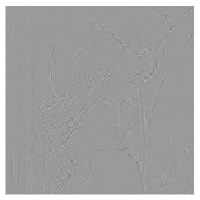
(f) proposed

(g) BAS-2010

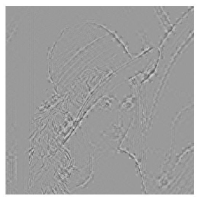
(h) WHT

Figure 5: Compressed images (a–d) and difference images (e–h) using the DCT, the proposed transform, the BAS-2010 approximation, and the WHT for the Lena image, considering $r=100$.

(a) DCT

(b) proposed

(c) BAS-2010

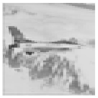
(d) WHT

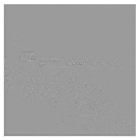
(e) DCT

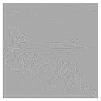
(f) proposed

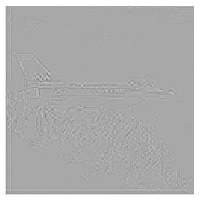
(g) BAS-2010

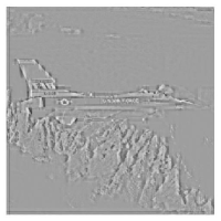
(h) WHT

Figure 6: Compressed images (a–d) and difference images (e–h) using the DCT, the proposed transform, the BAS-2010 approximation, and the WHT for the Airplane (F-16) image, considering $r=40$.

5 FPGA-based Hardware Implementation

In this section, the proposed DCT approximation and the BAS-2010 algorithm [10] were physically implemented on a field programmable gate array (FPGA) device. We employed the 40 nm CMOS Xilinx Virtex-6 XC6VLX240T FPGA for algorithm evaluation and comparison. Beforehand it is expected that the proposed algorithm exhibit modestly higher hardware demands. This is due to the fact that it requires 72 additions, whereas the BAS-2010 algorithms demands 64 additions.

We furnished circuit performance using metrics of (i) area ($A$) based on the quantity of required elementary programmable logic blocks (slices), the number of look-up tables (LUTs), and the flip-flops count, (ii) the speed, using the critical path delay ($T$), and (iii) the dynamic power consumption.

The number of occupied slices furnished an estimate of the on-chip silicon real estate requirement, whereas number of LUTs and flip-flops are the main logic resources available in a slice. In Xilinx FPGAs, a LUT is employed as a combinational function generator that can implement a given boolean function and a flip-flop is utilized as a 1-bit register. The critical path delay corresponds to the delay associated with the longest combinational path and directly governs the operating frequency of the hardware. The total power consumption of the hardware design constitutes of static and dynamic components. Static power consumption in FPGAs is dominated by the leakage power of the logic fabric and the configuration static RAM. Thus, is mostly design independent. On the other hand, the dynamic power consumption, which accounts for the dynamic power dissipation associated with clocks, logic blocks, and signals, provides a metric for the power efficiency of a given design [43]. The respective results are shown in Tables 3, 4, and 5, where the metrics corresponding to each design were measured for several choices of finite precision using input word length $W\in\{4,8,12,16\}$.

From Table 3, it is observed that the proposed design consumes $\approx 10\%$ more LUTs hardware resources than [10]. For $W=8$ the proposed design shows a $\approx 20\%$ increase in the number of slices consumed (and 10% more LUTs) while gaining 1-2 dB of improvement in PSNR compared to [10]. The increase in area shown by the proposed design has led to an increase in the critical path delay, area-time ($AT$), area-time-squared ($AT^{2}$) metrics and to a higher power consumption as indicated in Tables 4 and 5. Of particular interest is the case for $W=8$ input word size, where the proposed algorithm and hardware design shows a $5.7\%$ and $10\%$ increase in the critical path delay and dynamic power consumption, respectively, when compared to the algorithm in [10].

In this paper, we define a metric consisting of the product of error figures and the $AT$ value:

$$(\mbox{error figure})\times(\mbox{area-time product}).$$

The considered error figure can be the $1/\mbox{PSNR}$, MSE, $1/\mbox{UQI}$, or the total error energy, as given in Table 1. This metric aims at combining both the mathematical and the hardware aspects of the resulting implementation. The total error energy has the advantage of being image independent, being adopted in the combined metric. Considering the proposed architecture and [10], the obtained values for the combined metric are shown in Table 6.

Although the proposed DCT approximation consumes more resources than [10], a much better approximation for the exact DCT is achieved (see Table 1). This leads to superior compressed image quality (see Fig. 4). Indeed, the choice of algorithm is always a compromise between its mathematical properties, such as DCT proximity, energy error, and resulting image quality; and the related hardware aspects, such as area, speed, and power consumption. This implies our proposed algorithm is a better choice over [10] when picture quality is of higher importance.

Table 3: Area utilization for FPGA implementation.

Input	Area
word	BAS-2010 [10]			Proposed
length	Registers	LUTs	Slices	Registers	LUTs	Slices
4	403	543	172	597	524	178
8	828	704	241	956	909	290
12	1128	958	317	1253	1316	384
16	1432	1243	390	1597	1676	491

Table 4: Speed, $AT$, and $AT^{2}$ metrics for FPGA implementation.

Input word	Speed (MHz)		$AT$ ($\mbox{Slices}\cdot\mu s)$		$AT^{2}$ ($\mbox{Slices}\cdot{\mu s}^{2}\cdot 10^{-3}$)
length	BAS-2010 [10]	Proposed	BAS-2010 [10]	Proposed	BAS-2010 [10]	Proposed
4	369.13	342.9	0.466	0.519	1.26	1.51
8	361.92	342.114	0.666	0.848	1.84	2.48
12	363.63	336.813	0.872	1.140	2.40	3.38
16	341.29	338.18	1.143	1.452	3.35	4.29

Table 5: Dynamic power consumption for FPGA implementation.

Input	Dynamic Power (mW)
word	BAS-2010 [10]				Proposed
length	Clocks	Logic	Signals	Total	Clocks	Logic	Signals	Total
4	0.033	0.022	0.030	0.085	0.040	0.020	0.029	0.089
8	0.041	0.016	0.034	0.091	0.041	0.023	0.037	0.101
12	0.059	0.022	0.050	0.131	0.054	0.033	0.054	0.141
16	0.069	0.028	0.070	0.167	0.065	0.042	0.077	0.184

Table 6: Comparison of the cost associated with each design

Input	Combined metric
word length	BAS-2010 [10]	Proposed
4	31.22	4.19
8	44.62	6.85
12	58.42	9.21
16	76.57	11.73

6 Conclusion

This paper introduced a new 16-point DCT approximation. The proposed transform requires no multiplication or bit shifting operations, is orthogonal, and its matrix elements are only $\{-1,0,1\}$. Using spectral analysis methods described in [20, 15], we demonstrated that the proposed transform outperforms the WHT and the BAS-2010 as an approximation for the 16-point DCT. The proposed transform was considered into standard image compression methods. The resulting images were assessed for quality by means of PSNR, MSE, and UQI. According to these metrics, the proposed transform could outperform the WHT and the BAS-2010 approximation at any compression ratio. We also derived an efficient fast algorithm for the proposed matrix, which required 72 additions.

This algorithm was implemented in hardware and compared with a state-of-the-art 16-point DCT approximation [10]. FPGA-based rapid prototypes were designed, simulated, physically implemented, and tested for 4-, 8-, 12-, and 16-bit input data word sizes. A typical application having 8-bit input image data could be subject to 16-point DCT approximations at a real-time rate of $342\cdot 10^{6}$ transforms per second, for FPGA clock frequency of 342 MHz, leading to a pixel rate of $5.488\cdot 10^{9}$ pixels/second. Both proposed and BAS-2010 algorithms were realized on FPGA and tested and hardware metrics including area, power, critical path delay, and area-time complexity. Additionally, an extensive investigation of relative performance in both subjective mode as well as objective picture quality metrics using average PSNR, average MSE, and average UQI was produced. The proposed DCT approximation algorithm improves on the state-of-art algorithm in [10] by 1-2 dB for PSNR at the cost of only eight extra adders.

Video coding using motion partitions larger than 8$\times$8 pixels is investigated in [16, 47] with satisfactory application in H.264/AVC standard for video compression. In this perspective, the new proposed approximation transform is a candidate technique to image and video coding with block size equal to 16$\times$16. This blocklength is of particular importance in the emerging H.265 reconfigurable video codec standard [25].

References

- [1] N. Ahmed, T. Natarajan, and K. R. Rao. Discrete cosine transform. IEEE Transactions on Computers, C-23(1):90–93, Jan. 1974.
- [2] Y. Arai, T. Agui, and M. Nakajima. A fast DCT-SQ scheme for images. Transactions of the IEICE, E-71(11):1095–1097, 1988.
- [3] H. L. P. Arjuna Madanayake, R. J. Cintra, D. Onen, V. S. Dimitrov, and L. T. Bruton. Algebraic integer based 88 2-D DCT architecture for digital video processing. In Proceedings of the IEEE International Symposium on Circuits and Systems (ISCAS), pages 1247–1250, May 2011.
- [4] F. M. Bayer and R. J. Cintra. Image compression via a fast DCT approximation. IEEE Latin America Transactions, 8(6):708–713, Dec. 2010.
- [5] V. Bhaskaran and K. Konstantinides. Image and Video Compression Standards. Kluwer Academic Publishers, Boston, 1997.
- [6] G. Bi and Y. Zeng. Transforms and Fast Algorithms for Signal Analysis and Representations. Birkhäuser, 2004.
- [7] R. E. Blahut. Fast Algorithms for Digital Signal Processing. Addison-Wesley, 1985.
- [8] S. Bouguezel, M. O. Ahmad, and M. N. S. Swamy. Low-complexity 88 transform for image compression. Electronics Letters, 44(21):1249–1250, Sept. 2008.
- [9] S. Bouguezel, M. O. Ahmad, and M. N. S. Swamy. A fast 88 transform for image compression. In Proceedings of the 2009 Internation Conference on Microelectronics, 2009.
- [10] S. Bouguezel, M. O. Ahmad, and M. N. S. Swamy. A novel transform for image compression. In Proceedings of the 53rd IEEE International Midwest Symposium on Circuits and Systems (MWSCAS), 2010.
- [11] S. Bouguezel, M. O. Ahmad, and M. N. S. Swamy. A low-complexity parametric transform for image compression. In Proceedings of the 2011 IEEE International Symposium on Circuits and Systems, 2011.
- [12] V. Britanak, P. Yip, and K. R. Rao. Discrete Cosine and Sine Transforms. Academic Press, 2007.
- [13] W.-H. Chen, C. H. Smith, and S. C. Fralick. A fast computational algorithm for the discrete cosine transform. IEEE Transactions on Communications, COM-25(9):1004–1009, Sept. 1977.
- [14] N. I. Cho and S. U. Lee. Fast algorithm and implementation of 2-D discrete cosine transform. IEEE Transactions on Circuits and Systems, 38(3):297–305, Mar. 1991.
- [15] R. J. Cintra and F. M. Bayer. A DCT approximation for image compression. IEEE Signal Processing Letters, 18(10):579–582, Oct. 2011.
- [16] T. Davies, K. R. Andersson, R. Sjöberg, T. Wiegand, D. Marpe, K. Ugur, J. Ridge, M. Karczewicz, P. Chen, G. Martin-Cocher, K. McCann, W.-J. Han, G. Bjontegaard, and A. Fuldseth. Joint collaborative team on video coding (JCT-VC) of ITU-T SG16 WP3 and ISO/IEC JTC1/SC29/WG11: Suggestion for a test model. JCTVC-A033, International Telecommunication Union, Dresden, DE, Apr. 2010.
- [17] V. S. Dimitrov, K. Wahid, and G. A. Jullien. Multiplication-free DCT architecture using algebraic integer encoding. Electronics Letters, 40(20):1310–1311, 2004.
- [18] B. J. Fino. Relations between Haar and Walsh/Hadamard transforms. Proceedings of the IEEE, 60(5):647–648, May 1972.
- [19] R. C. Gonzalez and R. E. Woods. Digital Image Processing. Prentice Hall, Upper Saddle River, NJ, 2002.
- [20] T. I. Haweel. A new square wave transform based on the DCT. Signal Processing, 82:2309–2319, 2001.
- [21] H. S. Hou. A fast recursive algorithm for computing the discrete cosine transform. IEEE Transactions on Acoustic, Signal, and Speech Processing, 6(10):1455–1461, 1987.
- [22] International Organisation for Standardisation. Generic coding of moving pictures and associated audio information – Part 2: Video. ISO/IEC JTC1/SC29/WG11 - coding of moving pictures and audio, ISO, 1994.
- [23] International Telecommunication Union. ITU-T recommendation H.261 version 1: Video codec for audiovisual services at kbits. Technical report, ITU-T, 1990.
- [24] International Telecommunication Union. ITU-T recommendation H.263 version 1: Video coding for low bit rate communication. Technical report, ITU-T, 1995.
- [25] H. Kalva. The H.264 Video Coding Standard. IEEE Multimedia, 13(4):86–90, Oct. 2006.
- [26] S. M. Kay. Fundamentals of Statistical Signal Processing, Volume I: Estimation Theory, volume 1 of Prentice Hall Signal Processing Series. Prentice Hall, Upper Saddle River, NJ, 1993.
- [27] W.-K. Kuo and K.-W. Wu. Traffic prediction and QoS transmission of real-time live VBR videos in WLANs. ACM Transactions on Multimedia Computing, Communications and Applications, 7(4):36:1–36:21, Dec. 2011.
- [28] K. H. Lee, E. A. J. H. Park, W. J. Han, and J. H. Min. Technical considerations for ad hoc group on new challenges in video coding standardization. MPEG Doc. M15580, Hannover, Germany, July 2008.
- [29] K. Lengwehasatit and A. Ortega. Scalable variable complexity approximate forward DCT. IEEE Transactions on Circuits and Systems for Video Technology, 14(11):1236–1248, Nov. 2004.
- [30] J. Liang and T. D. Tran. Fast multiplierless approximations of the DCT with the lifting scheme. IEEE Transactions on Signal Processing, 49(12):3032–3044, Dec. 2001.
- [31] C. Loeffler, A. Ligtenberg, and G. Moschytz. Practical fast 1D DCT algorithms with 11 multiplications. In Proceedings of the International Conference on Acoustics, Speech, and Signal Processing, pages 988–991, 1989.
- [32] A. Luthra, G. J. Sullivan, and T. Wiegand. Introduction to the special issue on the H.264/AVC video coding standard. IEEE Transactions on Circuits and Systems for Video Technology, 13(7):557–559, July 2003.
- [33] H. S. Malvar, A. Hallapuro, M. Karczewicz, and L. Kerofsky. Low-complexity transform and quantization in H.264/AVC. IEEE Transactions on Circuits and Systems for Video Technology, 13(7):598–603, July 2003.
- [34] A. V. Oppenheim and R. W. Schafer. Discrete-Time Signal Processing. Prentice Hall, 3 edition, 2009.
- [35] I.-M. Pao and M.-T. Sun. Approximation of calculations for forward discrete cosine transform. IEEE Transactions on Circuits and Systems for Video Technology, 8(3):264–268, June 1998.
- [36] W. B. Pennebaker and J. L. Mitchell. JPEG Still Image Data Compression Standard. Van Nostrand Reinhold, New York, NY, 1992.
- [37] R. Piessens, E. deDoncker-Kapenga, C. Uberhuber, and D. Kahaner. Quadpack: a Subroutine Package for Automatic Integration. Springer-Verlag, 1983.
- [38] K. R. Rao and P. Yip. Discrete Cosine Transform: Algorithms, Advantages, Applications. Academic Press, San Diego, CA, 1990.
- [39] N. Roma and L. Sousa. Efficient hybrid DCT-domain algorithm for video spatial downscaling. EURASIP Journal on Advances in Signal Processing, 2007(2):30–30, 2007.
- [40] D. Salomon. Data Compression. Springer, 3 edition, 2004.
- [41] D. Salomon. The Computer Graphics Manual, volume 1. Springer-Verlag, London, UK, 2011.
- [42] S. Saponara. Real-time and low-power processing of 3D direct/inverse discrete cosine transform for low-complexity video codec. Journal of Real-Time Image Processing, 7:43–53, 2012. 10.1007/s11554-010-0174-5.
- [43] M. Shafique and J. Henkel. Background and related work. In Hardware/Software Architectures for Low-Power Embedded Multimedia Systems. Springer New York, 2011.
- [44] N. Suehiro and M. Hateri. Fast algorithms for the DFT and other sinusoidal transforms. IEEE Transactions on Acoustic, Signal, and Speech Processing, 34(6):642–644, 1986.
- [45] T. Suzuki and M. Ikehara. Integer DCT based on direct-lifting of DCT-IDCT for lossless-to-lossy image coding. IEEE Transactions on Image Processing, 19(11):2958–2965, Nov. 2010.
- [46] J. V. Team. Recommendation H.264 and ISO/IEC 14 496–10 AVC: Draft ITU-T recommendation and final draft international standard of joint video specification. Technical report, ITU-T, 2003.
- [47] Telecommunication Standardization Sector. Video coding using extended block sizes. COM 16-C 123-E, International Telecommunication Union, Jan. 2009.
- [48] The USC-SIPI image database. http://sipi.usc.edu/database, 2011. University of Southern California, Signal and Image Processing Institute.
- [49] Z. Wang and A. Bovik. A universal image quality index. IEEE Signal Processing Letters, 9(3):81–84, 2002.
- [50] Z. Wang, A. C. Bovik, H. R. Sheikh, and E. P. Simoncelli. Image quality assessment: from error visibility to structural similarity. IEEE Transactions on Image Processing, 13(4):600–612, Apr. 2004.
- [51] T. Wiegand, G. J. Sullivan, G. Bjontegaard, and A. Luthra. Overview of the H.264/AVC video coding standard. IEEE Transactions on Circuits and Systems for Video Technology, 13(7):560–576, July 2003.