Radial Contour Labeling with Straight Leaders

Abstract

The usefulness of technical drawings as well as scientific illustrations such as medical drawings of human anatomy essentially depends on the placement of labels that describe all relevant parts of the figure. In order to not spoil or clutter the figure with text, the labels are often placed around the figure and are associated by thin connecting lines to their features, respectively. This labeling technique is known as external label placement.

In this paper we introduce a flexible and general approach for external label placement assuming a contour of the figure prescribing the possible positions of the labels. While much research on external label placement aims for fast labeling procedures for interactive systems, we focus on highest-quality illustrations. Based on interviews with domain experts and a semi-automatic analysis of 202 handmade anatomical drawings, we identify a set of 18 layout quality criteria, naturally not all of equal importance. We design a new geometric label placement algorithm that is based only on the most important criteria. Yet, other criteria can flexibly be included in the algorithm, either as hard constraints not to be violated or as soft constraints whose violation is penalized by a general cost function. We formally prove that our approach yields labelings that satisfy all hard constraints and have minimum overall cost. Introducing several speedup techniques, we further demonstrate how to deploy our approach in practice. In an experimental evaluation on real-world anatomical drawings we show that the resulting labelings are of high quality and can be produced in adequate time.

1 Introduction

Atlases of human anatomy play a major role in the education of medical students and the teaching of medical terminology. Such books contain a broad spectrum of filigree and detailed drawings of the human anatomy from different cutaway views. For example, the third volume of the popular human anatomy atlas Sobotta [21] contains about 1200 figures on 384 pages. Figure 1 is one of them showing a cross section of the human skull. The usefulness of the figures essentially relies on the naming of the illustrated components. In order not to spoil the readability of the figure by occluding it with text, the names are placed around the figure without overlapping it. Thin black lines (which we call leaders) connecting the names with their features accordingly guarantee that the reader can match names and features correctly. Following preceding research, we call this labeling technique external label placement. In this paper we present a flexible and versatile approach for external label placement in figures. We use medical drawings as running example, but occlusion-free label placements are also indispensable for the readability of other highly detailed figures as they occur for example in scientific publications, mechanical engineering and maintenance manuals.

Besides readability also the aesthetics of the figures including their labelings play a central role in professional books. Each figure and its labels are subject to book-specific design rules. Our approach stands out by its ability to support an easy integration of these specific design rules. It particularly relies only on a few key assumptions that most figures with external label placement have in common. Other constraints and rules can easily be patched in according to demand.

Figure 1: Drawing labeled by our approach (variant TSCH, 34 sec.). Source: Paulsen, Waschke, Sobotta Atlas Anatomie des Menschen, 23.Auflage 2010 ©Elsevier GmbH, Urban & Fischer, München.

To validate our approach, we were in contact with both a layout artist and two editors of the human anatomy atlas Sobotta. Both the layout artist and the two editors stated that label placement is a mechanical, but extensively time-consuming task that is mainly done by hand. The tool support basically comprises simple operations such as placing text boxes and drawing line segments. Based on medical drawings annotated by the authors of the atlas for human anatomy, the layout artist creates the layout of each double page of the book. Using the annotated information, this includes arranging explanatory texts, figures, and labels around the figures. The interviewed layout artist stated that he needs about two hours to create the layout of a double page. Hereby, he spends a large portion of his time on label placement. Hence, with around 1200 figures in a single volume better tool support would clearly help in improving the process of creating such books. Further, with the upcoming applications on mobile devices, figures are deployed in differently scaled settings, which requires different external labelings for the same figure. Then, at the latest, automatic approaches become inevitable.

Related Work. External labeling algorithms have been investigated both from a practical and theoretical point of view. The practical results aim for fast and simple approaches that support heuristic optimizations for multiple criteria. These approaches are often targeted for interactive systems requiring a fast label placement procedure making compromises concerning quality. For example Hartmann et al. [14] and Ali et al. [2] both present models for external label placement listing a set of criteria concerning readability and aesthetics. They use these models to introduce simple force-based methods. Further strategies comprise iteratively rearranging labels [8], sequentially evaluating and placing labels by priority [13] or exploiting small spaces for label placement [11]. These approaches have in common that they are fast and simple, but quality guarantees can not be given. Hence, while they are customized to suit interactive systems, they can hardly serve as tools for a designer of professional books demanding complex design rules. Alternatively, the drawing criteria are transferred into an optimization problem based on a sophisticated mathematical model. Typically, such problems are not solved exactly, but by local optimization approaches. For example Vollick et al. [25] model external label placement by means of energy functions and apply simulated annealing. Stein and Décoret [22] use a simple greedy algorithm to find a solution for mathematical constraints. Further, Čmolík and Bittner [26] employ a greedy optimization using a model based on fuzzy logic. Mogalle et al. [18] also applied greedy optimization. The applications range from the interactive exploration of volume illustrations [8], over automatically annotated 2D slices of segmented structures [19], up to labeling explosion diagrams in augmented reality [24, 23].

In contrast, theoretical results mostly consider simple models, typically with one optimization criterion, e.g., minimizing the total leader length. Bekos et al. [6] introduced the first such model. Typically, it is assumed that the point features to be labeled are contained in a rectangle $R$ representing the boundary of the figure. The labels are placed outside that rectangle touching the boundary. It is assumed that the labels have uniform shapes and that their bounding boxes are already placed alongside $R$. Hence, the labeling problem basically becomes a geometric matching problem asking for a crossing-free assignment between the placed bounding boxes and the point features such that each point feature is connected with a unique bounding box by a leader. In a post-processing step the label texts are written into the bounding boxes, accordingly. This sub-problem of external labeling is called boundary labeling. The preceding research mostly differs in the choice of the parameters. Typically, the type of the leaders is broken down into straight-line leaders [6, 12, 9], L-shaped leaders [6, 7, 20, 17], S-shaped leaders [6, 4, 15] and leaders with a diagonal segment [7, 5]. Further, the results distinguish between the number of sides on which the labels may lie; on one, two or multiple sides of $R$. Typical optimization functions are minimizing the total leader length or minimizing the number of bends. Some of the approaches also allow general cost functions (e.g., [7]) applying dynamic programming. Recently, Fink and Suri [10] presented dynamic programming approaches for boundary labeling with uniform labels and rectangular boundaries using the four major leader types, which include straight-line leaders. For labels on two opposite sides of the rectangle, their approaches run in $O(n^{15})$ (fixed label candidates) and $O(n^{27})$ (non-fixed label candidates) time for straight-line leaders. A more detailed survey was recently given by Barth et al. [3], which also comprises a user-study showing that straight-line leaders and L-shaped leaders outperform the other mentioned leader types concerning readability. While the results on boundary labeling are interesting from a theoretical perspective, they are hardly applicable in realistic settings, where labels are not uniform and the boundary of the figure is not a rectangle.

Our Contribution. Our approach bridges the gap between the practical and theoretical results. Like many of the theoretical results, it uses a clearly and mathematically defined model to guarantee pre-defined design rules. However, in contrast to preceding research our approach is significantly more flexible in adapting other constraints. After introducing some terminology (Sect. 2) we present an extensive list of drawing criteria for external label placement. Our list of criteria contains and refines the quality criteria listed in previous work [14, 2] and identifies several more. We stress that, in contrast to previous work, our criteria are obtained directly from interviews with layout artists and editors of anatomical atlases. Moreover, we empirically verified the level of compliance with these criteria for 202 figures printed in the Sobotta [21] atlas (Sect. 3) using a semi-automatic quantitative analysis.

Based on a reasonable subset of the most important criteria we introduce a flexible formal model for contour labeling, which is a generalization of boundary labeling (Sect. 4). Afterwards we describe a basic dynamic programming approach that solves the mathematical problem optimally (Sect. 5). Our approach allows to include further drawing criteria both as hard and soft constraints, where hard constraints may not be violated at all and the compliance of soft constraints is rated by a cost function. Previous work rarely uses hard constraints and cannot easily include new hard constraints. Moreover, in contrast to previous algorithms that compute mathematical optimal solutions, our approach also takes consecutively placed labels into account. At first glance this seems to be a small improvement, but in fact it is important to obtain an appealing labeling where, for example, labels have regular distances or the angles of consecutive labels should be similar. Further, our approach supports labels of different sizes. Indeed, for each point feature, the user can pre-define a set of different label shapes, which do not need to be rectangles. This may be used to model different ways of text formatting supporting single and multi-line labels. Further, the user may specify for each label an individual set of candidate positions that is used for the label placement procedure. Moreover, the user may mark areas that are not allowed to be overlapped by labels including their leaders. This is important to avoid undesired overlaps with the figure or to integrate the figure along with its labeling into a double page with explanatory text. The approach also allows to pre-define groups of labels that are placed consecutively, which is required when naming features that are semantically related.

Our approach is not limited to the described features, but other criteria can be incorporated easily. The strength of our approach comes at the cost of a high asymptotic running time $O(n^{8})$, where $n$ describes the complexity of the input instance. Recently, Keil et al. [16] presented a similar general dynamic programming approach for computing an independent set in outerstring graphs, which can be utilized to solve contour labeling in $O(n^{6})$ time for a general cost function rating individual labels; however, it cannot take joint costs of two consecutive labels into account. In contrast to Fink and Suri [10] our approach is significantly faster ($O(n^{8})$ instead of $O(n^{15})$) and it supports non-uniform labels and more general shapes. With some engineering (Sect. 6) we can solve realistically sized instances in adequate time and high layout quality as is shown in our evaluation (Sect. 7) on a large benchmark set of real-world instances.

2 Terminology

Figure 2: Terminology. The radial ordering is given by the numbers placed closely to the text boxes.

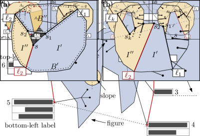
An illustration with external labeling consists of a figure as well as a set of labels outside of the figure naming single point features of the figure. Hereby a label consists of a text box that lies outside of the figure and a line segment connecting the text box with its point feature; see Fig. 2. We call the line segment the leader and the point feature the site of the label. More precisely, the text box is a rectangle containing a (possibly multi-line) text. Typically, the rectangle is not displayed, but it is used for the further description. We assume that the leader of a label ends on the boundary of the text box; we call that point the port of the label. A leader is directed from its site to its port. A label whose leader goes to the left is called a left label and a label whose leader goes to the right is called a right label. Analogously, a label is a top label (bottom label) if its leader goes upwards (downwards). The baseline of a bottom-right label is the horizontal half line that emanates from the bottom-right corner of the label’s text box to the right. For a top-right label the baseline is the horizontal half line that emanates from the top-right corner of the label’s text box to the right. The baselines for bottom-left and top-left labels are defined symmetrically. We define the slope of a leader is the clockwise angle (starting at 12 o’clock) between the leader and the vertical segment going through the connected site. A leader of a labeling intersects the contour of the figure at its exit point; in case that a leader intersects a figure multiple times, we regard the intersection point closest to the port. Traversing the figure’s boundary in clockwise order starting from the boundary’s topmost point defines an ordering on the exit points of the leaders and accordingly on the labels; we call this the radial ordering of the labeling. Two labels are consecutive if one directly follows the other in the radial ordering. The labeling contour is the polygon that connects the ports of the labels in the given radial ordering.

3 Drawing Criteria

Figure 3: Drawing criteria. (a) Criterion G3 (b) Criterion 5 (c) Criterion T5, which is violated by the red middle label. (d) Criterion L4, which is violated by Label 4 and Label 5.

We conducted interviews with domain experts (one layout artist and two editors of [21]) in order to extract a comprehensive set of important layout quality criteria as listed below. During these interviews, the experts explained how they typically proceed when labeling a single illustration. Further, they were asked to list layout criteria that they explicitly take into account. The extracted formal criteria were subsequently discussed using example illustrations printed in Sobotta [21].

Drawing criteria for sites.

1. Shape. Sites are represented by small points in the drawing.

2. Position. The position of a site is prescribed by domain experts and can be assumed to be fixed and given with the input.

3. Type. Either a site has its own label, or multiple sites have the same label. In the latter case the leaders are bundled forking at a certain point; see Label 5 in Fig. 2.

For simplicity, we assume that we only have sites of the first type, but with some engineering our algorithms can also be adapted to the second case. Now consider an external labeling of a medical drawing. We have extracted the following criteria.

General drawing criteria.

1. Externality. The text boxes of the labels are placed outside the drawing in the available areas.

2. Planarity. To sustain readability, labels may not overlap or intersect each other.

3. Simple shape. The labeling contour should be simple avoiding turning points; see Fig. 3(a).

4. Left/right side. The radial order of a labeling can be partitioned into a sequence of left labels and a sequence of right labels. Consequently, the labeling contour can be partitioned into a left labeling contour and a right labeling contour.

5. Similarity. The labeling contour mimics the contour of the figure such that small “indentations” of the figure are not taken into account; see Fig. 3(b).

6. Grouping. Labels may be required by the designer to appear consecutively in the radial ordering of the labeling.

Drawing criteria for text boxes.

1. Spacing. The vertical distances between text boxes are preferably uniform. Distances less than the height of one text line should be avoided, but may be admissible if not preventable.

2. Appearance. For all labels the same font is applied. Differences in the importance of labels may be expressed by different emphasis (bold, italic).

3. Single/Multi line. If possible, a text box should consist of a single-line text. Only due to the available space, text boxes may consist of multiple lines.

4. Ports. For left (right) labels the port lies on the right (left) edge of the text box in the vertical center of the first text line.

5. Staircase. Let $\ell_{1}$ and $\ell_{2}$ be two consecutive labels. Neither $\ell_{1}$ nor $\ell_{2}$ intersects the baseline of the other; see Fig. 3(c).

Drawing criteria for leaders.

1. Length. The part of a leader covering the figure should be (preferably) short.

2. Distinctiveness. Leaders running close together should not be parallel to avoid reader confusion.

3. Distance. Leaders preferably comply with a minimum distance to sites of other leaders.

4. Monotonicity. The slope of the leaders increases with respect to the radial ordering of the leaders; see Fig.3(d).

Typically a labeling does not fully satisfy all these criteria, but criteria may contradict each other requiring appropriate comprises. For example requiring monotonicity (L4) may enlarge the total leader length, which conflicts with criterion L1. Our approach is characterized by the fact that these compromises are not already made during the design of the labeling algorithm, but they lie in the hand of the layout artist applying the algorithm. Specifically, our approach only needs criteria S2, G1, G2, G4 and T5 as hard constraints not to be violated. Further, we assume that we are given a simple shape (G3) enclosing the figure and prescribing possible positions of ports. All other criteria are optional, but can be easily patched in as either hard or soft constraints as needed. Hereby the compliance of soft constraints is rated by means of a general cost function that can be defined when applying the algorithm. In our interviews the domain experts strongly emphasized the importance of G2 and G3. They further pointed out that labels should not be placed behind other labels, which we express by T5. We further analyzed 202 medical drawings of Sobotta [21] in a semi-automatic way. To that end we vectorized the images by extracting the text boxes, the leaders, the sites and the contour of the figure. More precisely, we computed the difference of two images showing the same object; one with labels and one without labels. From this difference we automatically extracted the contour of the figure, the text boxes and the ports of the leaders. The leaders were manually extracted. In case that a leader was connected to multiple sites, we have pragmatically extracted the leader only up to the first fork point $p$ and placed a single site at this point. In case that $p$ was not contained $\mathbb{F}$, we took the projection of $p$ on the boundary of $\mathbb{F}$ along the half-line from the port of $\lambda$ through $p$. The figures contain between $4$ and $64$ sites; see also Fig. 12.

All of these examples satisfy S1, G1, G2, G4, and T4. Further, 18 figures contain at least one set of labels that are explicitly grouped by a large curly brace (G6). Only a dwindling small percentage $(0.4\%)$ of all labels violate the staircase property (T5) and about $6.2\%$ violate monotonicity (L4). Since the other criteria are soft, we did not quantitatively check these in the semi-automatic analysis; yet, they are well founded in the conducted interviews.

4 Formal Model

We now describe a formal model for external label placement. We are given a simple polygon $\mathbb{F}$ that describes the contour of the figure and contains $n$ sites to be labeled. We denote the set of the sites by $\mathbb{S}$ and assume that the sites are in general position, i.e., no three sites are colinear. For each site $s\in\mathbb{S}$ we describe its label $\ell$ by a rectangle $r$ and an oriented line segment $\lambda$ that starts at $s$ and ends on the boundary of $r$. We call $\lambda$ the leader of $\ell$, $r$ the text box of $\ell$, and the end point of $\lambda$ on $r$ the port of $\ell$. The other end point is the site of $\ell$; see Fig. 2. In the following we only consider labels whose text boxes satisfy T4.

A set $\mathcal{L}$ of labels over $\mathbb{S}$ is called an external labeling of $(\mathbb{F},\mathbb{S})$, if (1) $|\mathcal{L}|=|\mathbb{S}|$, (2) for each site $s\in\mathbb{S}$ there is exactly one label in $\mathcal{L}$ that belongs to $s$, and (3) every text box of a label in $\mathcal{L}$ lies outside of $\mathbb{F}$. If no two labels in $\mathcal{L}$ intersect each other, $\mathcal{L}$ is planar . A labeling $\mathcal{L}$ is called a staircase labeling if it satisfies criterion T5.

Let $\mathcal{L}$ be a planar labeling. Let $\ell_{1},\dots,\ell_{n}$ be the labels of $\mathcal{L}$ in the radial ordering. For simplicity we define $\ell_{n+1}:=\ell_{1}$. The cost $c$ of a labeling $\mathcal{L}$ is defined as $c(\mathcal{L})=\sum_{i=1}^{n}c_{1}(\ell_{i})+c_{2}(\ell_{i},\ell_{i+1})$, where $c_{1}$ is a function assigning a cost to a single label $\ell_{i}$ and $c_{2}$ is a function assigning a cost to two consecutive labels $\ell_{i}$ and $\ell_{i+1}$. We note that in contrast to previous research the cost function also supports rating two consecutive labels, which is crucial to set labels in relation with each other. Given the cost function $c$, the problem ExternalLabeling then asks for a planar labeling $\mathcal{L}$ of $(\mathbb{F},\mathbb{S})$ that has minimum cost with respect to $c$, i.e., for any other planar labeling $\mathcal{L}^{\prime}$ of $(\mathbb{F},\mathbb{S})$ it holds $c(\mathcal{L})\leq c(\mathcal{L}^{\prime})$.

We consider the special case that the ports of the labels lie on a common contour enclosing $\mathbb{F}$. In contrast to classical boundary labeling, which assumes a rectangular figure, this contour schematizes the shape of the figure with a certain offset; in Section 7 we shortly describe how to construct a reasonable contour. Thus, the contour describes the common silhouette formed by the labels. We assume that the contour is given as a simple polygon $\mathbb{C}$ enclosing $\mathbb{F}$. An external labeling $\mathcal{L}$ is called a contour labeling if for every label of $\mathcal{L}$ its leader lies inside $\mathbb{C}$ and its port lies on the boundary $\partial\mathbb{C}$ of $\mathbb{C}$. Since not every part of $\mathbb{C}$’s boundary may be suitable for the placement of labels, we require that the ports of the labels are contained in a given subset $\mathbb{P}\subseteq\partial\mathbb{C}$ of candidate ports. If $\mathbb{P}$ is finite, the input instance has fixed ports and otherwise sliding ports.

Observation 1.

In a planar contour labeling the ports of the labels induce the same radial ordering with respect to $\mathbb{C}$ as the exit points of the labels with respect to $\mathbb{F}$.

A tuple $\mathbb{I}=(\mathbb{C},\mathbb{S},\mathbb{P})$ is called an instance of contour labeling. The region of $\mathbb{I}$ is the region enclosed by $\mathbb{C}$. We restrict ourselves to convex contours and clearly separated sites and text boxes as follows implementing Criteria G1 and G3, respectively.

Assumption 1.

The contour $\mathbb{C}$ is convex and no text box of any label intersects the convex hull of $\mathbb{S}$.

For all of the 202 analyzed medical drawings it holds that no text box of any label intersects the convex hull of $\mathbb{S}$.

Due to the convexity of $\mathbb{C}$, the contour can be uniquely split into a left and right side described by two maximal $y$-monotone chains $\mathbb{C}_{\mathrm{L}}$ and $\mathbb{C}_{\mathrm{R}}$, respectively. The next assumption implements Criterion G4.

Assumption 2.

A left label has its port on $\mathbb{C}_{\mathrm{L}}$ and a right label has its port on $\mathbb{C}_{\mathrm{R}}$.

Given a cost function $c$, the problem ContourLabeling then asks for an (cost) optimal, planar staircase contour labeling $\mathcal{L}$ of $(\mathbb{C},\mathbb{S},\mathbb{P})$ with respect to $c$, i.e., for any other planar staircase contour labeling $\mathcal{L}^{\prime}$ of $(\mathbb{C},\mathbb{S},\mathbb{P})$ it holds that $c(\mathcal{L})\leq c(\mathcal{L}^{\prime})$.

5 Algorithmic Core

In this section we describe how to construct the optimal labeling $\mathcal{L}$ of a given instance $(\mathbb{C},\mathbb{S},\mathbb{P})$ with respect to a given cost function $c$. To that end we apply a dynamic programming approach. The basic idea is that any optimal contour labeling can be recursively decomposed into a set of sub-labelings inducing disjoint sub-instances. As we show later, these sub-instances are specially formed; we call them convex sub-instances. We further show that any such sub-instance can be described by a constant number of parameters over $\mathbb{S}$ and $\mathbb{P}$. Hence, enumerating all choices of these parameters, we can enumerate in polynomial time all possible convex sub-instances that an optimal labeling may consist of. For each such sub-instance we compute the cost of an optimal labeling reusing the results of already computed values of smaller sub-instances. In this way we obtain the value of the optimal labeling for the given instance. Summarizing, our approach consists of four steps.

Step 1. Compute all possible convex sub-instances by enumerating all possible choices defined over $\mathbb{S}$ and $\mathbb{P}$.

Step 2. In increasing order of the number of contained sites, compute the optimal cost for each convex sub-instance $\mathbb{I}$. More precisely, to compute the optimal cost of $\mathbb{I}$ consider all possibilities how $\mathbb{I}$ can be composed of at most two smaller convex sub-instances.

Step 3. Consider all possibilities how the input instance can be described by a convex sub-instance. Among these, take the convex sub-instance with optimal cost.

Step 4. Starting with the resulting sub-instance of Step 3, apply a standard backtracking approach for dynamic programming to construct the corresponding labeling with optimal costs.

In the remainder of this section we explain the approach in more detail. In Section 5.1, we first prove some structural properties on contour labelings. These properties are crucial for the dynamic programming approach, which we describe in Section 5.2.

5.1 Structural Properties of Contour Labelings

The intersection of two labels is characterized by three types: the two leaders intersect, the two text boxes intersect or the leader of one label intersects the text box of the other label. The following lemma allows us to find planar labelings by avoiding leader-leader intersections and intersections between two consecutive labels.

Figure 4: Illustration of proof for Lemma 1.

Lemma 1.

Let $\mathbb{I}$ be an instance of ContourLabeling and let $\mathcal{L}$ be a staircase contour labeling of $\mathbb{I}$. If no pair of leaders intersect and if no two consecutive labels intersect, then $\mathcal{L}$ is planar.

Proof.

We prove that $\mathcal{L}$ is planar by systematically excluding the possible types of intersections.

Text-box–text-box intersection. Assume that there are two labels $\ell$ and $\ell^{\prime}$ that are not consecutive and whose text boxes intersect. The labels either lie on the same side or on different sides of $\mathbb{C}$.

First consider the case that $\ell$ and $\ell^{\prime}$ belong to different sides; without loss of generality let $\ell$ be a left label and $\ell^{\prime}$ be a right label. Due to T4, text boxes of $\ell$ and $\ell^{\prime}$ may only intersect if the port $p$ of $\ell$ lies to the right of the port $p^{\prime}$ of $\ell^{\prime}$. Since $p$ lies on $\mathbb{C}_{\mathrm{L}}$ and $p^{\prime}$ lies on $\mathbb{C}_{\mathrm{R}}$, this contradicts the convexity of $\mathbb{C}$.

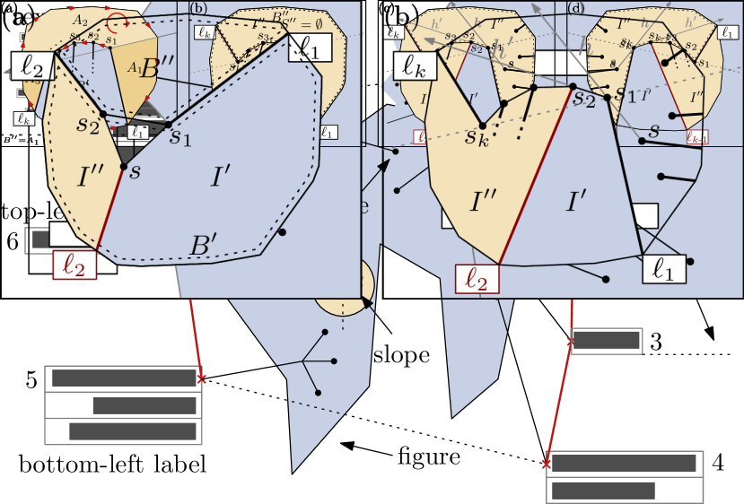
Now consider the case that $\ell$ and $\ell^{\prime}$ belong to the same side; without loss of generality let both be left labels; see Fig. 4(a). For intersecting each other, one of both labels intersects the base line of a left label in between both labels contradicting Criterion T5.

Text-box–leader intersection. Now assume that there is a label $\ell$ whose text box is intersected by the leader $\lambda^{\prime}$ of another label $\ell^{\prime}$; see Fig. 4(b). We denote the ports of $\ell$ and $\ell^{\prime}$ by $p$ and $p^{\prime}$ respectively. Further, let $t$ be the first intersection point of $\lambda^{\prime}$ with $\ell$ going along $\lambda^{\prime}$. We choose $\ell^{\prime}$ such that there is no other leader intersecting $\ell$’s boundary $c$ between $p$ and $t$. Let $R$ be the region that is bounded by the boundary of $\ell$ from $p$ to $t$, the line segment $\overline{tp^{\prime}}$, and the boundary $c^{\prime}$ of $\mathbb{C}$ from $p^{\prime}$ to $p$. Since $\ell$ and $\ell^{\prime}$ are not consecutive, there is a label $\ell^{\prime\prime}$ with port $p^{\prime\prime}$ on $c^{\prime}$. The site $s^{\prime\prime}$ of $\ell^{\prime\prime}$ lies in $R$ because otherwise the leader of $\ell^{\prime\prime}$ intersects $c$ or the segment $\overline{tp^{\prime}}$. Due to the convexity of $\mathbb{C}$, the segment $\overline{s^{\prime}s^{\prime\prime}}$ is contained in $\mathbb{C}$. Since $s^{\prime}$ lies in the complement of $R$, the segment $\overline{s^{\prime}s^{\prime\prime}}$ intersects $c$, which implies that $\ell$ intersects the convex hull of $\mathbb{S}$ contradicting Assumption 1. ∎

Figure 5: Decomposition in convex instance $\mathbb{I}^{\prime}$ (blue) and concave instance $\mathbb{I}^{\prime\prime}$ (orange). (a) Illustration of basic definitions. (b) Type $A$ instance with $k>2$. (c) Type $B$ instance with $k>2$. (d) Capstone instance.

In the following, we show that each instance can be subdivided into a finite set of sub-instances of three types. We describe a sub-instance by a simple polygon that consists of two polylines. One polyline is part of the original contour $\mathbb{C}$ and the other polyline consists of a convex chain of sites and two leaders. More precisely, assume that we are given a convex chain $K=(s_{1},\ldots,s_{k})$ of sites with $k\geq 2$ and the two non-intersecting labels $\ell_{1}$ and $\ell_{k}$ of $s_{1}$ and $s_{k}$, respectively; see Fig. 5(a). The directed polyline $K^{\prime}=(p_{1},s_{1},\dots,s_{k},p_{k})$ splits the polygon $\mathbb{C}$ into two polygons $\mathbb{C}^{\prime}$ and $\mathbb{C}^{\prime\prime}$, where $p_{1}$ and $p_{k}$ are the ports of $\ell_{1}$ and $\ell_{k}$, respectively. We consider the order of the sites such that we meet $p_{1}$ before $p_{k}$ when going along the contour of $\mathbb{C}$ in clockwise-order starting at the top of $\mathbb{C}$. Further, going along $K^{\prime}$ we denote the sub-polygon to the left of $K^{\prime}$ by $\mathbb{C}^{\prime}$ and to the right of $K^{\prime}$ by $\mathbb{C}^{\prime\prime}$. With respect to the direction of $K^{\prime}$, the sub-polygon $\mathbb{C}^{\prime}$ is counter-clockwise oriented, while $\mathbb{C}^{\prime\prime}$ is clockwise oriented. Further, $\mathbb{C}^{\prime\prime}$ contains the top point of $\mathbb{C}$. We define that $\mathbb{C}^{\prime}$ contains the sites $s_{2},\dots,s_{k-1}$, while $\mathbb{C}^{\prime\prime}$ does not contain them.

Thus, the polyline $K^{\prime}$ partitions the instance $(\mathbb{C},\mathbb{S},\mathbb{P})$ into two sub-instances $\mathbb{I}^{\prime}=(\mathbb{C}^{\prime},\mathbb{S}^{\prime},\mathbb{P}^{\prime})$ and $\mathbb{I}^{\prime\prime}=(\mathbb{C}^{\prime\prime},\mathbb{S}^{\prime\prime},\mathbb{P}^{\prime\prime})$ such that

1. $\mathbb{S}^{\prime}\cup\mathbb{S}^{\prime\prime}=\mathbb{S}\setminus\{s_{1},s_{k}\}$ and $\mathbb{P}^{\prime}\cup\mathbb{P}^{\prime\prime}=\mathbb{P}\setminus\{p_{1},p_{k}\}$,

2. the sites of $\mathbb{S}^{\prime}$ lie in $\mathbb{C}^{\prime}$ or on $K$ and the sites of $\mathbb{S}^{\prime\prime}$ lie in the interior of $\mathbb{C}^{\prime\prime}$,

3. the ports of $\mathbb{P}^{\prime}$ lie on the boundary of $\mathbb{C}^{\prime}$ and the ports of $\mathbb{P}^{\prime\prime}$ lie on the boundary of $\mathbb{C}^{\prime\prime}$.

Note that the sites $s_{1}$, $s_{k}$ and the ports $p_{1}$, $p_{k}$ neither belong to $\mathbb{I}^{\prime}$ nor to $\mathbb{I}^{\prime\prime}$, because they are already used by the fixed labels $\ell_{1}$ and $\ell_{k}$. We call $(\ell_{1},\ell_{k},K)$, which defines the polyline $K^{\prime}$, the separator of $\mathbb{C}^{\prime}$ and $\mathbb{C}^{\prime\prime}$. For two sub-instances we say that they are disjoint if the interiors of their regions are disjoint.

In the following, we only consider sub-instances in which the convex chain $K$ lies to the right of the line $l$ through $s_{1}$ and $s_{k}$ pointing towards $s_{k}$ from $s_{1}$; we will show that these are sufficient for decomposing any instance. Put differently, the chain $K$ is a convex part of the boundary of $\mathbb{C}^{\prime}$ and a concave part of the boundary of $\mathbb{C}^{\prime\prime}$. We call $\mathbb{I}^{\prime}$ a convex sub-instance and $\mathbb{I}^{\prime\prime}$ a concave sub-instance.

The line $l$ splits $\mathbb{C}^{\prime\prime}$ into three regions $A_{1}$, $A_{2}$ and $A_{3}$; see Fig. 5(a). Let $A_{2}$ be the region to the right of $l$ and let $A_{1}$ and $A_{3}$ be the regions to the left of $l$ such that $A_{1}$ is adjacent to the leader of $\ell_{1}$ and $A_{3}$ is adjacent to the leader of $\ell_{k}$. Depending on the choice of $\ell_{1}$ and $\ell_{k}$, the regions $A_{1}$ and $A_{3}$ may or may not exist. We call $\mathbb{C}^{\prime\prime}$ the exterior of $\mathbb{C}^{\prime}$ and vice versa. We distinguish the following convex instances.

1. A convex instance has type A if there is a site $s\in A_{1}$ such that $\ell_{1}$ and the half-line $h$ emanating from $s$ through $s_{1}$ separates $K$ from the sites in $\mathbb{C}^{\prime\prime}$; see Fig 5(b).

2. A convex instance has type B if there is a site $s\in A_{3}$ such that $\ell_{k}$ and the half-line $h$ emanating from $s$ through $s_{k}$ separates $K$ from the sites in $\mathbb{C}^{\prime\prime}$; see Fig 5(c).

For both types the chain $K$ is uniquely defined by the choice of $\ell_{1}$, $\ell_{k}$ and $s$. Thus, type A and type B instances are uniquely defined by $\ell_{1}$, $\ell_{k}$ and $s$; we denote these instances by $\mathbb{I}_{\mathrm{A}}[\ell_{1},\ell_{k},s]$ and $\mathbb{I}_{\mathrm{B}}[\ell_{1},\ell_{k},s]$, respectively. We call $s$ the support point of the instance. In case that $\mathbb{C}^{\prime\prime}$ is empty, the chain $K$ is already uniquely defined by $\ell_{1}$ and $\ell_{k}$ and we write $\mathbb{I}_{\mathrm{A}}[\ell_{1},\ell_{k},\bot]$ and $\mathbb{I}_{\mathrm{B}}[\ell_{1},\ell_{k},\bot]$. Hence, we can enumerate all such instances by enumerating all possible triples consisting of two labels and one site. Since each label is defined by one port and one site, we obtain $O(|\mathbb{S}|^{3}\dot{|}\mathbb{P}|^{2})$ instances in total. Note that instances of type B are symmetric to type A instances.

For $k=2$ the chain consists of the sites $s_{1}$ and $s_{2}$ and the support point is superfluous; such an instance is solely defined by the labels $\ell_{1}$ and $\ell_{2}$ of $s_{1}$ and $s_{2}$, respectively. We call these instances capstone instances and denote them by $\mathbb{I}_{\mathrm{C}}[\ell_{1},\ell_{2}]$; see Fig. 5(d).

We now show that any labeling can be composed into instances of these three types. We say that an instance is empty if its set $\mathbb{S}$ of sites is empty. For a labeling $\mathcal{L}$ of an instance $\mathbb{I}$ we write $\mathcal{L}\raise-0.86108pt\hbox{$|$}_{\mathbb{I}^{\prime}}$ for the labeling $\mathcal{L}^{\prime}\subseteq\mathcal{L}$ that is restricted to the sites and ports of the sub-instance $\mathbb{I}^{\prime}$ of $\mathbb{I}$. Let $(\ell_{1},\ell_{k},K)$ denote the separator of $\mathbb{I}^{\prime}$. For a labeling $\mathcal{L}^{\prime}$ of a sub-instance $\mathbb{I}^{\prime}$ we require that any leader of any label $\ell$ in $\mathcal{L}^{\prime}$ lies in the contour of the sub-instance not intersecting the separator (the sites $s_{2},\dots,s_{k-1}$ are excluded from this restriction). In that case we say that $\ell$ is contained in $\mathbb{I}^{\prime}$. We further emphasize that the labels $\ell_{1}$ and $\ell_{k}$ are contained in $\mathcal{L}^{\prime}$, but they are fixed describing the contour of $\mathbb{I}^{\prime}$ so that their sites and ports do not belong to the sites and ports of $\mathbb{I}^{\prime}$, respectively. The next lemma states how to decompose type A and type B instances into smaller type A, type B and capstone instances. Fig. 6(a) illustrates Case (i). Case (ii) is symmetric to Case (i).

Figure 6: Decomposition of a convex instance $\mathbb{I}$ (dashed polygon). (a) Type A instance with $k>2$ is decomposed into capstone instance $\mathbb{I}^{\prime}$ and type A instance $\mathbb{I}^{\prime\prime}$. (b) Capstone instance is decomposed into two smaller capstone instances. (c)–(d) Capstone instance is decomposed into type A and type B instances.

Lemma 2.

Let $\mathbb{I}$ be a convex instance with separator $(\ell_{1},\ell_{k},K=(s_{1},\dots,s_{k}))$ and $k>2$. Further, let $\mathcal{L}$ be a planar labeling of $\mathbb{I}$.

1. If $\mathbb{I}$ has type $A$, the label $\ell_{2}\in\mathcal{L}$ of $s_{2}$ splits $\mathbb{I}$ into the disjoint sub-instances $\mathbb{I}^{\prime}=\mathbb{I}_{\mathrm{C}}[\ell_{1},\ell_{2}]$ and $\mathbb{I}^{\prime\prime}=\mathbb{I}_{\mathrm{A}}[\ell_{2},\ell_{k},s_{1}]$ such that any label $\ell\in\mathcal{L}$ is contained in $\mathbb{I}^{\prime}$ or $\mathbb{I}^{\prime\prime}$.

   $$c(\mathcal{L})=c(\mathcal{L}\raise-0.86108pt\hbox{$|$}_{\mathbb{I}_{\mathrm{C}}[\ell_{1},\ell_{2}]})+c(\mathcal{L}\raise-0.86108pt\hbox{$|$}_{\mathbb{I}_{\mathrm{A}}[\ell_{2},\ell_{k},s_{1}]})-c_{1}(\ell_{2})$$

2. If $\mathbb{I}$ has type $B$, the label $\ell_{k-1}\in\mathcal{L}$ of $s_{k-1}$ splits $\mathbb{I}$ into the two disjoint sub-instances $\mathbb{I}^{\prime}=\mathbb{I}_{\mathrm{C}}[\ell_{k-1},\ell_{k}]$ and $\mathbb{I}^{\prime\prime}=\mathbb{I}_{\mathrm{B}}[\ell_{1},\ell_{k-1},s_{k}]$ such that any label $\ell\in\mathcal{L}$ is contained in $\mathbb{I}^{\prime}$ or $\mathbb{I}^{\prime\prime}$.

   $$c(\mathcal{L})=c(\mathcal{L}\raise-0.86108pt\hbox{$|$}_{\mathbb{I}_{\mathrm{C}}[\ell_{k-1},\ell_{k}]})+c(\mathcal{L}\raise-0.86108pt\hbox{$|$}_{\mathbb{I}_{\mathrm{B}}[\ell_{1},\ell_{k-1},s_{k}]})-c_{1}(\ell_{k-1})$$

Proof.

We only argue for type A instances. Symmetric arguments hold for type B instances. Consider an arbitrary sub-instance $\mathbb{I}=(\mathbb{C},\mathbb{S},\mathbb{P})$ of type A; see Fig. 6(a). Since $\ell_{2}$ connects two points of $\mathbb{C}$’s boundary, it partitions $\mathbb{I}$ into two sub-instances $\mathbb{I}^{\prime}$ and $\mathbb{I}^{\prime\prime}$ with labelings $\mathcal{L}\raise-0.86108pt\hbox{$|$}_{\mathbb{I}^{\prime}}$ and $\mathcal{L}\raise-0.86108pt\hbox{$|$}_{\mathbb{I}^{\prime\prime}}$ such that any label of $\mathcal{L}\setminus\{\ell_{2}\}$ either is contained in $\mathbb{I}^{\prime}$ or $\mathbb{I}^{\prime\prime}$. Let $\mathbb{I}^{\prime}$ be the instance containing $s_{1}$ and $\mathbb{I}^{\prime\prime}$ the other one. Obviously, $\mathbb{I}^{\prime}$ forms the capstone instance $\mathbb{I}_{\mathrm{C}}[\ell_{1},\ell_{2}]$. We now show that $\mathbb{I}^{\prime\prime}$ forms instance $\mathbb{I}^{\prime\prime}=\mathbb{I}_{\mathrm{A}}[\ell_{2},\ell_{k},s_{1}]$ of type A.

By definition of $\mathbb{I}$ the label $\ell_{1}$ and the half-line $h$ emanating from $s$ through $s_{1}$ separates the convex chain $K$ of $\mathbb{I}$ from the sites in the exterior of $\mathbb{I}$. Because of the convexity of $K$, the half-line $h^{\prime}$ emanating from $s_{1}$ through $s_{2}$ and the label $\ell_{2}$ separate the convex chain $K^{\prime}=(s_{2},\dots,s_{k})$ from the sites in the exterior of $\mathbb{I}^{\prime\prime}$. Hence, $\mathbb{I}^{\prime\prime}=\mathbb{I}_{\mathrm{A}}[\ell_{2},\ell_{k},s_{1}]$ has type A.

The cost of $\mathcal{L}$ is composed of the costs of $\mathcal{L}\raise-0.86108pt\hbox{$|$}_{\mathbb{I}^{\prime}}$ and $\mathcal{L}\raise-0.86108pt\hbox{$|$}_{\mathbb{I}^{\prime\prime}}$ as follows $c(\mathcal{L})=c(\mathcal{L}\raise-0.86108pt\hbox{$|$}_{\mathbb{I}_{\mathrm{C}}[\ell_{1},\ell_{2}]})+c(\mathcal{L}\raise-0.86108pt\hbox{$|$}_{\mathbb{I}_{\mathrm{A}}[\ell_{2},\ell_{k},s_{1}]})-c_{1}(\ell_{2})$. To not count $\ell_{2}$ twice, we subtract $c_{1}(\ell_{2})$. ∎

The convex sub-instances $\mathbb{I}^{\prime}$ and $\mathbb{I}^{\prime\prime}$ of the previous lemma contain fewer sites than $\mathbb{I}$. Thus, recursively applying Lemma 2 decomposes $\mathbb{I}$ into a set of type A and type B instances until all instances are capstone instances. The next lemma states how to decompose capstone instances into smaller type A, type B and capstone instances. Fig. 6(b) illustrates Case (ii), Fig. 6(c) illustrates Case (iii), Case (iv) is symmetric to Case (iii) and Fig. 6(d) illustrates Case(v).

Lemma 3.

Let $\mathbb{I}=\mathbb{I}_{\mathrm{C}}[\ell_{1},\ell_{2}]$ be a capstone instance with separator $(\ell_{1},\ell_{2},K=(s_{1},s_{2}))$. Further, let $\mathcal{L}$ be a planar labeling of $\mathbb{I}$. One of the following statements applies for $\mathbb{I}$.

1. The instance $\mathbb{I}$ is empty.

   $$c(\mathcal{L})=c_{1}(\ell_{1})+c_{1}(\ell_{2})+c_{2}(\ell_{1},\ell_{2})$$

2. There is a label $\ell$ in $\mathcal{L}$ such that any label in $\mathcal{L}$ is contained in one of the two disjoint capstone instances $\mathbb{I}_{\mathrm{C}}[\ell_{1},\ell]$ and $\mathbb{I}_{\mathrm{C}}[\ell,\ell_{2}]$.

   $$c(\mathcal{L})=c(\mathcal{L}\raise-0.86108pt\hbox{$|$}_{\mathbb{I}_{\mathrm{C}}[\ell_{1},\ell]})+c(\mathcal{L}\raise-0.86108pt\hbox{$|$}_{\mathbb{I}_{\mathrm{C}}[\ell,\ell_{2}]})-c_{1}(\ell)$$

3. There is a label $\ell\in\mathcal{L}$ s.t. any label in $\mathcal{L}$ is contained in $\mathbb{I}_{\mathrm{A}}[\ell_{1},\ell,s_{2}]$.

   $$c(\mathcal{L})=c(\mathcal{L}\raise-0.86108pt\hbox{$|$}_{\mathbb{I}_{\mathrm{A}}[\ell_{1},\ell,s_{2}]})+c_{2}(\ell,\ell_{2})$$

4. There is a label $\ell\in\mathcal{L}$ s.t. any label in $\mathcal{L}$ is contained in $\mathbb{I}_{\mathrm{B}}[\ell,\ell_{2},s_{1}]$.

   $$c(\mathcal{L})=c(\mathcal{L}\raise-0.86108pt\hbox{$|$}_{\mathbb{I}_{\mathrm{B}}[\ell,\ell_{2},s_{1}]})+c_{2}(\ell_{1},\ell)$$

5. There are labels $\ell,\ell^{\prime}\in\mathcal{L}$ with $\ell\neq\ell^{\prime}$ s.t. any label in $\mathcal{L}$ is contained in either $\mathbb{I}_{\mathrm{A}}[\ell_{1},\ell,s_{2}]$ or $\mathbb{I}_{\mathrm{B}}[\ell^{\prime},\ell_{2},s_{1}]$.

   $$c(\mathcal{L})=c(\mathcal{L}\raise-0.86108pt\hbox{$|$}_{\mathbb{I}_{\mathrm{A}}[\ell_{1},\ell,s_{2}]})+c(\mathcal{L}\raise-0.86108pt\hbox{$|$}_{\mathbb{I}_{\mathrm{B}}[\ell^{\prime},\ell_{2},s_{1}]})+c_{2}(\ell,\ell^{\prime})$$

Proof.

If $\mathbb{I}=(\mathbb{C},\mathbb{S},\mathbb{P})$ is empty, the cost of $\mathcal{L}$ are composed by $c(\mathcal{L})=c_{1}(\ell_{1})+c_{2}(\ell_{2})+c_{2}(\ell_{1},\ell_{2})$, which yields Case (i).

So assume that $\mathbb{I}$ is not empty. The line $l$ through $s_{1}$ and $s_{2}$ splits $\mathbb{C}$ into three regions $A_{1}$, $A_{2}$ and $A_{3}$; see Fig. 6(b). Let $A_{2}$ be the region to the left of $l$ (going along $l$) and let $A_{1}$ and $A_{3}$ be the regions to the right of $l$ such that $A_{1}$ and $A_{3}$ are adjacent to the leaders of $\ell_{1}$ and $\ell_{2}$, respectively. Further, let $p_{1}$ and $p_{2}$ be the ports of $\ell_{1}$ and $\ell_{2}$, respectively.

First assume that there is a site $s$ with label $\ell\in\mathcal{L}$ such that the separating triangle $\Delta(s_{1},s,s_{2})$ lies in $\mathbb{C}$ and its interior is not intersected by any label in $\mathcal{L}$; the triangle must lie in $A_{2}$. Together with $\ell$, it partitions $\mathbb{I}$ into the two sub-instances $\mathbb{I}^{\prime}$ and $\mathbb{I}^{\prime\prime}$. They form the capstone instances $\mathbb{I}^{\prime}=\mathbb{I}_{\mathrm{C}}[\ell_{1},\ell]$ and $\mathbb{I}^{\prime\prime}=\mathbb{I}_{\mathrm{C}}[\ell,\ell_{2}]$ as in Case (ii). It is easy to see that $c(\mathcal{L})=c(\mathcal{L}\raise-0.86108pt\hbox{$|$}_{\mathbb{I}_{\mathrm{C}}[\ell_{1},\ell]})+c(\mathcal{L}\raise-0.86108pt\hbox{$|$}_{\mathbb{I}_{\mathrm{C}}[\ell,\ell_{2}]})-c_{1}(\ell).$ We subtract $c_{1}(\ell)$ to not count $\ell$ twice.

So assume that there is no such separating triangle, which implies that $A_{1}\cup A_{3}$ contains sites. If this were not the case, $A_{2}$ would contain a site, because $\mathbb{I}$ is not empty. Among these sites we easily could find a site forming a separating triangle. In particular due to Assumption 1 such a triangle cannot be intersected by any text box. We distinguish three cases how $A_{1}$ and $A_{3}$ contain sites.

Case: $A_{1}$ contains a site, but $A_{3}$ is empty. Let $s$ be a site in $A_{1}$. We denote its label by $\ell$ and the port of $\ell$ by $p$. We choose $s$ and $\ell$ such that no label of any site in $A_{1}$ succeeds $\ell$ in the radial ordering. Let $K$ be the convex chain of sites in $A_{1}$ such that $K$ starts at $s_{1}$, ends at $s$, and any site in $A_{1}$ lies in the counterclockwise oriented polygon $\mathbb{C}^{\prime}$ defined by $p_{1}$, $K$, $p$ and the part of $\mathbb{C}$ in between $p$ and $p_{1}$; see Fig. 6(c). All sites in $A_{2}$ also lie in $\mathbb{C}^{\prime}$, because otherwise we could find a separating triangle. Hence, the clockwise oriented polygon $\mathbb{C}^{\prime\prime}$ defined by $p_{2}$, $s_{2}$, $s_{1}$, $K$, $p$ and the part of $\mathbb{C}$ in between $p$ and $s_{2}$ does not contain any site. By the choice of $\ell$ all labels must be contained in the instance induced by $\mathbb{C}^{\prime}$. In particular the half-line $h$ emanating from $s_{2}$ through $s_{1}$ separates $K$ from the sites in the exterior of $\mathbb{I}^{\prime}$. Hence $\mathbb{I}^{\prime}$ is the type A instance $\mathbb{I}_{\mathrm{A}}[\ell_{1},\ell,s_{2}]$. This yields Case (iii) and $c(\mathcal{L})=c(\mathcal{L}\raise-0.86108pt\hbox{$|$}_{\mathbb{I}_{\mathrm{A}}[\ell_{1},\ell,s_{2}]})+c_{2}(\ell,\ell_{2}).$

Case: $A_{3}$ contains a site, but $A_{2}$ is empty. Symmetrically, we construct a type B instance $\mathbb{I}^{\prime}=\mathbb{I}_{\mathrm{B}}[\ell,\ell_{2},s_{1}]$, which yields Case (iv).

Case: Both $A_{1}$ and $A_{2}$ contain sites. Combining the construction of the previous two cases, we obtain two labels $\ell$ and $\ell^{\prime}$ that define the type A and type B instances $\mathbb{I}^{\prime}=\mathbb{I}_{\mathrm{A}}[\ell_{1},\ell,s_{2}]$ and $\mathbb{I}^{\prime\prime}=\mathbb{I}_{\mathrm{B}}[\ell^{\prime},\ell_{2},s_{1}]$ of case (v); see Fig. 6(d). ∎

Lemma 2 and Lemma 3 describe how to decompose an arbitrary convex sub-instance $\mathbb{I}$ into a set of empty capstone instances. The next lemma implies that any labeling of any instance $\mathbb{I}$ of ContourLabeling can be decomposed into empty capstone instances.

Lemma 4.

Let $\mathbb{I}$ be an instance of ContourLabeling and let $\mathcal{L}$ be a planar labeling of $\mathbb{I}$. The first leader $\ell$ and the last leader $\ell^{\prime}$ in the radial ordering of $\mathcal{L}$ define a type A instance $\mathbb{I}^{\prime}=\mathbb{I}_{\mathrm{A}}[\ell,\ell^{\prime},\bot]$ such that the exterior of $\mathbb{I}^{\prime}$ is empty and $c(\mathcal{L})=c(\mathcal{L}\raise-0.86108pt\hbox{$|$}_{\mathbb{I}^{\prime}})+c_{2}(\ell,\ell^{\prime}).$

Figure 7: Illustration of Lemma 4

Figure 8: Illustration of Bundles.

Proof.

Let $\mathbb{I}=(\mathbb{C},\mathbb{S},\mathbb{P})$. Further, let $s$ and $s^{\prime}$ be the sites and let $p$ and $p^{\prime}$ be the ports of the two labels $\ell$ and $\ell^{\prime}$, respectively. The polyline $(p,s,s^{\prime},p^{\prime})$ partitions $\mathbb{C}$ into two sub-polygons; see Fig. 8. Let $\mathbb{C}^{\prime}$ be the counterclockwise oriented polygon and $\mathbb{C}^{\prime\prime}$ be the clockwise oriented polygon. Let $\mathbb{S}^{\prime\prime}$ be the sites in $\mathbb{C}^{\prime\prime}$. The port of any label in $\mathcal{L}$ lies on the boundary of $\mathbb{C}^{\prime}$, because otherwise $\ell$ and $\ell^{\prime}$ would not be the first and last labels in the radial ordering of $\mathcal{L}$, respectively. Hence, any leader of any label with site in $\mathbb{S}^{\prime\prime}$ must intersect the line segment $\overline{ss^{\prime}}$. This in particular implies that any of these sites must lie to the right of the line $l$ that goes through $s$ and $s^{\prime}$ in that direction. Let $H$ be the convex hull of $\mathbb{S}^{\prime\prime}\cup\{s,s^{\prime}\}$. Removing $\overline{ss^{\prime}}$ from $H$, we obtain the desired convex chain $K$, which lies to the right of $l$. Together with $\ell$ and $\ell^{\prime}$ it forms the type A instance $\mathbb{I}_{\mathrm{A}}[\ell,\ell^{\prime},\bot]$. ∎

5.2 Dynamic Programming

Applying the results of the previous section we present a dynamic programming approach that solves ContourLabeling with fixed ports optimally. For type A, type B and capstone instances the approach creates the three tables $T_{\mathrm{A}}$, $T_{\mathrm{B}}$ and $T_{\mathrm{C}}$ storing the optimal costs of the considered instances, respectively. We call an instance valid if the two labels $\ell_{1}$ and $\ell_{k}$ defining the separator do not intersect and comply with T5.

Step 1. We compute all valid instances of type A and type B, and all valid capstone instances.

Step 2. We compute the optimal costs for all convex sub-instances. Let $\mathbb{I}$ be the currently considered instance of size $i\geq 0$ with separator $(\ell_{1},\ell_{k},K=(s_{1},\cdots,s_{k}))$, where the size of $\mathbb{I}$ is the number of sites contained in $\mathbb{I}$; recall that $s_{1}$ and $s_{k}$ do not belong to $\mathbb{I}$. Considering the instances in non-decreasing order of their sizes, we can assume that we have already computed the optimal costs for all convex instances with size less than $i$. We distinguish the two main cases $k=2$ and $k>2$.

Case $\mathbf{k=2.}$ The instance $\mathbb{I}$ forms the capstone instance $\mathbb{I}_{\mathrm{C}}[\ell_{1},\ell_{2}]$. Let $s_{1}$ and $s_{2}$ be the sites of $\ell_{1}$ and $\ell_{2}$, respectively. Following Lemma 3 we apply five steps.

1. If $\mathbb{I}_{\mathrm{C}}[\ell_{1},\ell_{2}]$ is not empty, we set $w_{1}:=\infty$ and otherwise

   $$w_{1}:=c_{1}(\ell_{1})+c_{1}(\ell_{2})+c_{2}(\ell_{1},\ell_{2}).$$

2. We consider every site $s$ in $\mathbb{I}_{\mathrm{C}}[\ell_{1},\ell_{2}]$ such that the separating triangle $\Delta(s_{1},s_{2},s)$ lies in the region of $\mathbb{I}$ and does not contain any other site. For all such sites we determine each label candidate $\ell$ that partitions $\mathbb{I}$ into valid disjoint capstone instances $\mathbb{I}_{\mathrm{C}}[\ell_{1},\ell]$ and $\mathbb{I}_{\mathrm{C}}[\ell,\ell_{2}]$. Let $D$ denote the set of all those labels.

   $$w_{2}:=\min_{\ell\in D}T_{\mathrm{C}}[\ell_{1},\ell]+T_{\mathrm{C}}[\ell,\ell_{2}]-c_{1}(\ell).$$

3. We determine every label $\ell$ of $\mathbb{I}_{\mathrm{C}}[\ell_{1},\ell_{2}]$ such that every site of $\mathbb{I}$ lies in $\mathbb{I}_{\mathrm{A}}[\ell_{1},\ell,s_{2}]$. Let $D$ denote the set of those labels.

   $$w_{3}:=\min_{\ell\in D}T_{\mathrm{A}}[\ell_{1},\ell,s_{2}]+c_{2}(\ell,\ell_{2}).$$

4. We determine every label $\ell$ of $\mathbb{I}_{\mathrm{C}}[\ell_{1},\ell_{2}]$ such that every site of $\mathbb{I}$ lies in $\mathbb{I}_{\mathrm{B}}[\ell,\ell_{2},s_{1}]$. Let $D$ denote the set of those labels.

   $$w_{4}:=\min_{\ell\in D}T_{\mathrm{B}}[\ell,\ell_{2},s_{1}]+c_{2}(\ell_{1},\ell).$$

5. We determine every pair $(\ell,\ell^{\prime})$ of intersection-free labels of $\mathbb{I}_{\mathrm{C}}[\ell_{1},\ell_{2}]$ such that every site of $\mathbb{I}[\ell_{1},\ell_{2}]$ lies in $\mathbb{I}_{\mathrm{A}}[\ell_{1},\ell,s_{2}]$ or $\mathbb{I}_{\mathrm{B}}[\ell^{\prime},\ell_{2},s_{1}]$. Let $D$ denote the set of those pairs labels.

   $$w_{5}:=\min_{(\ell,\ell^{\prime})\in D}T_{\mathrm{A}}[\ell_{1},\ell,s_{2}]+T_{\mathrm{B}}[\ell^{\prime},\ell_{2},s_{1}]+c_{2}(\ell,\ell^{\prime}).$$

In any of the above cases we choose the labels of the candidate set $D$ such that the considered instances are valid. Further, if $D$ is empty in sub-step ($i$), we set $w_{i}:=\infty$ ($2\leq i\leq 5$). We set $T_{\mathrm{C}}[\ell_{1},\ell_{2}]:=\min_{1\leq i\leq 5}\{w_{i}\}$.

Case $\mathbf{k>2.}$ Following Lemma 2 we distinguish two sub-cases. If $\mathbb{I}$ is a type $A$ instance $\mathbb{I}_{\mathrm{A}}[\ell_{1},\ell_{k},s]$ (where possibly $s=\bot$), we determine every possible label $\ell$ for site $s_{2}$. Let $D$ be the set of those labels. If $D$ is empty, we set $T_{\mathrm{A}}[\ell_{1},\ell_{k},s]:=\infty$ and otherwise

$$T_{\mathrm{A}}[\ell_{1},\ell_{k},s]:=\min_{\ell\in D}T_{\mathrm{C}}[\ell_{1},\ell]+T_{\mathrm{A}}[\ell,\ell_{k},s_{1}]-c_{1}(\ell).$$

If $\mathbb{I}$ has type B, we analogously define $D$ for $s_{k-1}$. If $D$ is empty, we set $T_{\mathrm{B}}[\ell_{1},\ell_{k},s]:=\infty$ and otherwise

$$T_{\mathrm{B}}[\ell_{1},\ell_{k},s]:=\min_{\ell\in D}T_{\mathrm{C}}[\ell,\ell_{k}]+T_{\mathrm{B}}[\ell_{1},\ell,s_{k}]-c_{1}(\ell).$$

In any of the cases above we call the elements in $D$ the descendants of the given instance.

Step 3. After computing the optimal costs of all convex instances, we enumerate all possible choices $(\ell,\ell^{\prime})$ of first and last labels in the radial ordering. Let $D$ denote the set of those choices. By Lemma 4 any choice $(\ell,\ell^{\prime})\in D$ forms a convex type A instance $\mathbb{I}^{\prime}=\mathbb{I}_{\mathrm{A}}[\ell,\ell^{\prime},\bot]$. Hence, the optimal cost $\textsc{OPT}(\mathbb{I})$ of $\mathbb{I}$ are

$$\textsc{OPT}(\mathbb{I})=\min_{(\ell,\ell^{\prime})\in D}T_{\mathrm{A}}[\ell,\ell^{\prime},\bot]+c_{2}(\ell,\ell^{\prime}).$$

Recall that if the convex chain $K$ of $\mathbb{I}^{\prime}$ has length 2, then we have $\mathbb{I}^{\prime}=\mathbb{I}_{\mathrm{C}}[\ell,\ell^{\prime}]$ and therefore $T_{\mathrm{A}}[\ell,\ell^{\prime},\bot]=T_{\mathrm{C}}[\ell,\ell^{\prime}]$. If $\textsc{OPT}(\mathbb{I})=\infty$, we return that $\mathbb{I}$ does not admit a contour labeling.

Step 4. Also storing the according descendants for each instance, we apply a standard backtracking approach for dynamic programming to obtain the corresponding labeling $\mathcal{L}$.

Theorem 1.

For an instance $\mathbb{I}=(\mathbb{C},\mathbb{S},\mathbb{P})$ contour labeling, the problem ContourLabeling can be solved in $O(|\mathbb{S}|^{4}|\mathbb{P}|^{4})$ time.

Proof.

We first show the correctness and then argue the running time. Let $\mathbb{I}$ be an arbitrary instance of ContourLabeling.

Correctness. Let $\mathcal{L}$ be a labeling constructed by our algorithm. We first show that $\mathcal{L}$ is planar proving the conditions of Lemma 1.

By construction we ensure that for a convex instance $\mathbb{I}$ the labels of $\mathbb{I}$’s separator comply with T5. In particular this implies that any two consecutive labels in $\mathcal{L}$ comply with T5, which implies that $\mathcal{L}$ is a staircase labeling. When computing the descendants $D$ for an instance, we ensure that $D$ does not contain any label that intersects the separator of that instance. By induction this implies that no leader in $\mathcal{L}$ intersects any other leader in $\mathcal{L}$. Further, we ensure that no two consecutive labels intersect. Hence, by Lemma 1 the labeling $\mathcal{L}$ is planar.

Finally, we prove that $\mathcal{L}$ is an optimal labeling of $\mathbb{I}$. By Lemma 2, 3 and 4 any labeling can be recursively decomposed into type A, type B, and capstone instances. Our algorithm enumerates all these instances. For each such instance $\mathbb{I}^{\prime}$ we search for the label(s) $\ell$ ($\ell^{\prime}$) that split $\mathbb{I}^{\prime}$ into smaller type A, type B and capstone instances. Since we enumerate all such labels, we also find the label minimizing the cost of $\mathbb{I}^{\prime}$.

Running Time. We now analyze the running time step by step.

Step 1. We create all possible convex instances of type A and type B, and all capstone instances by (conceptually) enumerating all tuples $(\ell_{1},\ell_{2})$ and $(\ell_{1},\ell_{2},s)$, where $\ell_{1}$ and $\ell_{2}$ are labels based on the ports and sites of $\mathbb{I}$ and $s\in S$. Since each label is defined by a site and a port, we enumerate $O(|\mathbb{S}|^{3}\cdot|\mathbb{P}|^{2})$ tuples. For each instance we also compute the convex chain $K$ and the sites contained in the instance, which needs $O(|\mathbb{S}|)$ time assuming that the sites are sorted by their $x$-coordinates. Sorting the instances by size needs $O(|\mathbb{S}|^{3}\cdot|\mathbb{P}|^{2}(\log|\mathbb{S}|+\log|\mathbb{P}|))$ time.

Step 2. Handling a single capstone instance we need $O(|\mathbb{S}|^{2}|\mathbb{P}|^{2})$ time: For the cases (1)–(4) there are $O(|\mathbb{S}|\cdot|\mathbb{P}|)$ descendants, while for case (5) there are $O(|\mathbb{S}|^{2}\cdot|\mathbb{P}|^{2})$ descendants. Since we consider $O(|\mathbb{S}|^{2}\cdot|\mathbb{P}|^{2})$ many instances, we obtain $O(|\mathbb{S}|^{4}|\mathbb{P}|^{4})$ running time in total for capstone instances.

Handling a single type A or type B instance there are $O(|\mathbb{P}|)$ descendants, because the site of the descendants is fixed. Since we consider $O(|\mathbb{S}|^{3}\cdot|\mathbb{P}|^{2})$ such instances, we obtain $O(|\mathbb{S}|^{3}|\mathbb{P}|^{3})$ running time, which is dominated by handling the capstone instances.

Step 3. Enumerating all pairs of first and last labels in the radial ordering can be done in $O(|\mathbb{S}|^{2}|\mathbb{P}|^{2})$ time.

Step 4. Storing for each instance its descendant of lowest cost, we can do backtracking in linear time.

Altogether, Step 2 dominates with $O(|\mathbb{S}|^{4}|\mathbb{P}|^{4})$ running time. ∎

The criteria mentioned in Section 3 can be easily patched into the approach. If a criterion should become a hard constraint not to be violated, we simply exclude any sub-instance violating this specific criterion. For example, to enforce monotonicity (L4) we remove any sub-instance whose defining labels violate this criterion. Similarly, if the criterion should become a soft-constraint, we do not exclude the sub-instance, but include its compliance with this criterion into its cost—provided that it can be modeled by the cost functions $c_{1}$ or $c_{2}$. This is true for all criteria listed in Section 3.

6 Algorithm Engineering

Initial experiments showed that a naive implementation of the dynamic programming approach does not yield reasonable running times, which matches the high asymptotic running times. In this section, we therefore describe how the approach can be implemented efficiently to prevent these problems for instances of realistic input sizes of $|S|\leq 70$.

6.1 Bundling

Instead of considering each possible label individually, we bundle labels and redefine the different types of instances based on bundles instead of single labels. More precisely, consider two labels $\ell_{1}$ and $\ell_{2}$ of the same site $s$ such that $\ell_{1}$ precedes $\ell_{2}$ in the radial ordering; see Fig. 8. Let $p_{1}$ and $p_{2}$ be the ports of $\ell_{1}$ and $\ell_{2}$, respectively. Further, let $R$ be the region enclosed by $\ell_{1}$, $\ell_{2}$ and the part of the contour $\mathbb{C}$ that lies between $p_{1}$ and $p_{2}$ (going in clockwise direction around $\mathbb{C}$). We call $\ell_{1}$ and $\ell_{2}$ equivalent if the region $R$ does not contain any site. Hence, $\ell_{1}$ can be slid along $\mathbb{C}$ to $\ell_{2}$ without passing any other site. A bundle of $s$ is a set $B$ of labels of $s$ that are pairwise equivalent. A set $B$ is maximal if there is no bundle $B^{\prime}$ with $B\subsetneq B^{\prime}$. We order the labels according their radial ordering. To ease the description we assume without loss of generality that there is no bundle that contains the top point of $\mathbb{C}$; we can split bundles at the top point of $\mathbb{C}$, if necessary.

As presented in Section 5.1 we describe a sub-instance $\mathbb{I}_{\mathrm{A}}[\ell,\ell^{\prime},t]$ ($\mathbb{I}_{\mathrm{B}}[\ell,\ell^{\prime},t]$, $\mathbb{I}_{\mathrm{C}}[\ell,\ell^{\prime}]$) by two labels $\ell$ and $\ell^{\prime}$ and by a support point $t$. We now generalize this concept to bundles. For two bundles $B$ and $B^{\prime}$ of two sites $s$ and $s^{\prime}$ the instance set $\textsc{Is}_{\mathrm{A}}[B,B^{\prime},t]$ contains every instance $\mathbb{I}_{\mathrm{A}}[\ell,\ell^{\prime},t]$ with $\ell\in B$ and $\ell^{\prime}\in B^{\prime}$. We analogously define the sets $\textsc{Is}_{\mathrm{B}}$ and $\textsc{Is}_{\mathrm{C}}$. Using these instance sets, we speed up the steps of our algorithm without losing optimality as follows.

Step 1. Instead of creating every instance of every type, we create all possible instance sets $\textsc{Is}_{\mathrm{A}}$, $\textsc{Is}_{\mathrm{B}}$ and $\textsc{Is}_{\mathrm{C}}$ based on the maximal bundles of the input instance. We note that we do not compute the instance sets explicitly, but each such set Is is uniquely described by the two labels that occur first and last in Is with respect to the radial ordering. Since any two instances of an instance set contain the same sites, we only compute these contained sites once per instance set. We further exclude any instance set that does not permit a labeling at all. To that end, we test whether there is enough space along the enclosed contour for all labels.

Step 2 & Step 3. Instead of computing the optimal cost for each individual instance, we iteratively compute lower and upper bounds of the optimal cost of the instance sets and refine these until we obtain the optimal cost.

More precisely, in each iteration we compute for each instance set Is a lower bound $L$ and an upper bound $U$ for the optimal costs of the instances in Is, i.e., for each instance $\mathbb{I}\in\textsc{Is}$ it holds $L\leq\textsc{OPT}(\mathbb{I})\leq U$. To that end we define for two bundles $B$ and $B^{\prime}$ the cost functions $c_{1}$ and $c_{2}$ as follows.

$$c_{1}(B)= (\min_{\ell\in B}c_{1}(\ell),\max_{\ell\in B}c_{1}(\ell))$$

$$c_{2}(B,B^{\prime})= (\min_{\ell\in B,\ell^{\prime}\in B^{\prime}}c_{2}(\ell,\ell^{\prime}),\max_{\ell\in B,\ell^{\prime}\in B^{\prime}}c_{2}(\ell,\ell^{\prime}))$$

Interpreting the result of $c_{1}(B)$ and $c_{2}(B,B^{\prime})$ as two-dimensional vectors we compute the tables $T_{\mathrm{A}}$, $T_{\mathrm{B}}$ and $T_{\mathrm{C}}$ in the same manner as before, but this time we use instance sets instead of instances and bundles instead of single labels. We analogously adapt Step 3.

Hence, we obtain for each instance set lower and upper bounds. In particular we obtain a lower bound $\bar{L}$ and an upper bound $\bar{U}$ for the given input instance. In case that $\bar{L}=\infty$, the input instance does not admit a labeling and we can abort the algorithm. Otherwise, we collect all instance sets of Step 3 whose lower bound does not exceed $\bar{U}$ and start a standard backtracking procedure to collect all instance sets whose lower bound does not exceed $\bar{U}$. Any other instance set is omitted, because it cannot be part of the optimal solution. Afterwards, we split each bundle $B$ into two half-sized bundles $B_{1}$ and $B_{2}$, i.e., let $\ell_{1},\dots,\ell_{h}$ be the labels in $B$ with respect to the radial ordering. We then set $B_{1}=\{\ell_{1},\dots,\ell_{m}\}$ and $B_{2}=\{\ell_{m+1},\dots,\ell_{h}\}$ where $m=\lfloor\frac{h}{2}\rfloor$. Thus, based on those new bundles we obtain new corresponding instance sets. We start the next iteration with the newly created instance sets.

We repeat this procedure until each bundle contains exactly one label. Thus, the bounds $\bar{L}$ and $\bar{U}$ equal the optimal cost of the input instance. Doing backtracking we construct the according labeling.

Figure 9: Shells (blue). (a) The label $\ell$ does not directly strive outwards and disturbs the overall appearance of the drawing. (b) No label candidate $\ell^{\prime}$ of $s^{\prime}$ can intersect the separating triangle $\Delta(s_{1},s_{2},s)$ without intersecting a shell of higher level.

6.2 Shells

We now describe two adaptations that further accelerate the approach. In contrast to the previous section these techniques do not necessarily preserve optimality. In Section 7 we show that in practice our heuristics achieve near-optimal solutions in reasonable time.

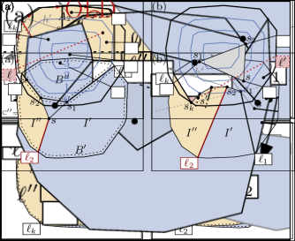
We observe that leaders typically point outwards without passing through the center of the figure; see Fig. 9(a). This guarantees short leader lengths and leaders fit in the overall appearance of the figure. We use this as follows. Based on the contour $\mathbb{C}$ we construct a set of offset polygons in the interior of $\mathbb{C}$ such that they have a pre-defined distance to each other; see Fig. 9(a). We call these polygons shells. The level of a shell is the number of shells containing that shell and the level of a site is the level of the innermost shell containing $s$.

We require for every site that its leader does not intersect a shell with higher level. Hence, we can exclude any label that violates this requirement. The more shells are used the more labels are excluded improving the running time. However, it also becomes more likely that the optimal labeling gets lost. In our experiments we have chosen the shells such that less than $0.9\%$ of the labels in handmade drawings violate this property; see also Section 7.

We further speed up Step 2(2). To that end let $\mathbb{I}_{\mathrm{C}}[\ell_{1},\ell_{2}]$ be the currently considered capstone instance and let $s_{1}$ and $s_{2}$ be the sites of $\ell_{1}$ and $\ell_{2}$, respectively. Further, let $D$ be the set of descendants. We only consider descendants that have a level that is at least as high as the level of $s_{1}$ and $s_{2}$. If such descendants do not exist, we take those with highest level. In case that the shells are convex and nested this particular adaption does not have any impact on the achievable cost, because for any such site $s$ the triangle $\Delta(s_{1},s_{2},s)$ is contained in the shell of $s_{1}$, $s_{2}$ or $s$. It therefore cannot be intersected by any leader of a descendant with a site that has a lower level; see Fig. 9(b).

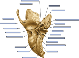Contour & Shells	Original
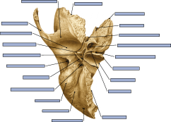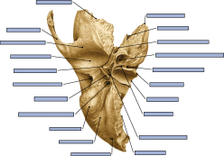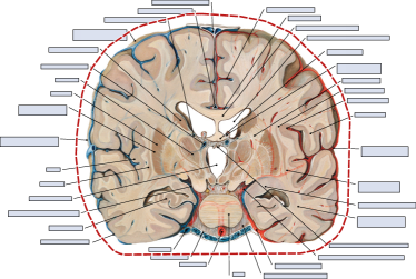
OPT (10 sec.), CH (7 sec.)	SCH (2 sec.), TSCH (1 sec.)

Figure 10: OPT and CH as well as SCH and TSCH produced the same labelings, respectively. Source: Paulsen, Waschke, Sobotta Atlas Anatomie des Menschen, 23.Auflage 2010 ©Elsevier GmbH, Urban & Fischer, München.

6.3 Miscellaneous

We can further speed-up the approach as follows.

Simple-Instances. Initial experiments showed that non-capstone instances are more of theoretical interests proving the optimality of the approach, but typically the optimal labeling can be decomposed into capstone instances. Hence, it lends itself to only consider capstone instances; particularly Step 2(3)–(5) are omitted. The asymptotic running time remains the same, because handling capstone instances dominates the running time.

One-Sided-Instances. Assuming criterion G4 we can apply the following speed-up technique preserving the optimality of our approach. Consider a capstone instance $\mathbb{I}_{\mathrm{C}}[\ell_{1},\ell_{2}]$ such that both labels $\ell_{1}$ and $\ell_{2}$ are right labels. Let $D$ be the descendants computed in Step 2(2). Indeed we only need to consider the descendants in $D$ with the leftmost site $s$ among all those descendants. It preserves optimality, because no descendant in $D$ of any other site can intersect the separating triangle $\Delta(s_{1},s_{2},s)$; due to criterion G4 they all lie to the right of the vertical line through $s$. Here $s_{1}$ and $s_{2}$ are the sites of $\ell_{1}$ and $\ell_{2}$. Symmetrically, we can apply the same technique for left labels $\ell_{1}$ and $\ell_{2}$ and the descendants with the rightmost site among all descendants in $D$. The asymptotic running time remains the same, because handling capstone instances with left and right labels dominates the running time.

Small-Triangles. Computing the set $D$ of descendants of a capstone instance $\mathbb{I}_{\mathrm{C}}[\ell_{1},\ell_{2}]$ in Step 2(2), any site $s$ in $\mathbb{I}_{\mathrm{C}}[\ell_{1},\ell_{2}]$ is considered that forms an empty separating triangle $\Delta(s_{1},s_{2},s)$. Hereby $s_{1}$ and $s_{2}$ are the sites of $\ell_{1}$ and $\ell_{2}$. For this speed-up technique we only consider the site $s$ with smallest triangle $\Delta(s_{1},s_{2},s)$ among those sites reducing the number of descendants in $D$. This improves the asymptotic running time by a factor of $O(n)$.

Contour & Shells	Original
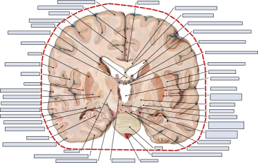
OPT (10 sec.), SCH (2 sec.)	TSCH (1 sec.)

Figure 11: OPT, CH and SCH produced the same labelings. With an cost ratio of $10.2$, the labeling produced by TSCH is an outlier; the labels distances are quite small. Source: Paulsen, Waschke, Sobotta Atlas Anatomie des Menschen, 23.Auflage 2010 ©Elsevier GmbH, Urban & Fischer, München.

7 Experimental Evaluation

We have implemented a prototype of our approach incorporating the speed-up techniques of Section 6. For simplicity we constructed the contour of the figure based on its convex hull $H$, i.e., the contour $\mathbb{C}$ is an exterior offset polygon of $H$ with distance of $25$ pixels. More sophisticated approaches can be applied [25]. Similarly, the shells are interior offset polygons of the contour having distance of $70$ pixels to the next shell. Both choices are ad-hoc values that mimic handmade drawings, but a designer may select them depending on the actual figure. Further, we placed ports by sampling the contour every 10 pixels.

Figure 12: Quality. Each column represents one figure broken down into the labelings computed by the algorithm OPT (blue rectangle), CH (green disk), SCH (pink diamond) or TSCH (orange triangle). X-axis: The figures are sorted by their number of sites in increasing order. Y-axis: not solved: Labelings that could not be constructed. not optimal: Cost ratio of non-optimal labelings. optimal: Any labeling $\mathcal{L}_{A}$ with $c(\mathcal{L}_{A})=c(\mathcal{L}_{\textsc{OPT}})$. Hereby $A\in\{\textsc{CH},\textsc{SCH},\textsc{TSCH},\textsc{OPT}\}$. Symbols of labelings violating monotonicity (L4) are enlarged and stabbed by a dashed vertical line.

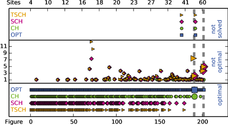
The implemented algorithm uses bundles, the speed-up of one-sided instances, and parallelizes Step 1; see Sect. 6. We distinguish the following variants of our algorithm:

1. Optimal (OPT): No further speed-up techniques.

2. Capstone-Heuristic (CH): Restricted to capstones.

3. Simple-Shell-Heuristic (SCH): Same as CH, but also shells are applied.

4. Triangle-Heuristic (TSCH): Same as SCH, but also including Small-Triangles.

The implementation was done in C++ and compiled with GCC 4.8.5 using optimization level O2. Further, unless specified otherwise, the experiments were performed on an Intel Xeon E5-1630v3 processor clocked at 3.7 GHz, with 128 GB of RAM.

We used the 202 extracted medical drawings as input data. For reasonably defining the cost functions $c_{1}$ and $c_{2}$, we first created six labelings for each of five selected figures. These labelings varied in the choice of minimum label distances, as well as enforcing monotonicity (L4) or not. We discussed these 30 labelings with a domain expert. She confirmed that monotonicity is an important criterion to obtain balanced labelings and rated the labelings best where labels with less than 30 pixels distance were penalized. Smaller and larger penalty thresholds were rated worse. Further, the expert emphasized that leaders should not run past sites too closely. Figures 1, 10 and 11 show three example illustrations labeled with our algorithms. Further example illustrations are found on http://i11www.iti.kit.edu/contourlabeling/.

The analysis of handmade labelings also supports monotonicity: $93.8\%$ of the labels satisfy this property. For about $70\%$ of the test instances violating monotonicity, the violation was less than $10^{\circ}$ in maximum. About $93\%$ of these instances have at most $5$ violations.

We incorporated these findings into the cost function as follows. Let $M$ be a big constant. Any label candidate and any instance with cost at least $M$ is excluded. In our experiments we set $M=10^{9}$. The cost function $c_{1}$ takes the leader’s length and the smallest distance to sites into account. More precisely, any candidate label whose leader is three times longer than the shortest possible leader for the same site is excluded. Hence, sites located close to the contour of the figure have short leaders, while sites in the center of the figure are not affected by this exclusion at all. Let $\ell$ be a label candidate and $\lambda$ be the leader of $\ell$. If the distance $d$ of $\lambda$ to any site (not connected to $\lambda$) is less than 10 pixels, we set $c_{1}(\ell)=\operatorname{length}(\lambda)^{2}+M/(100\cdot d)$ and otherwise $c_{1}(\ell)=\operatorname{length}(\lambda)^{2}$. Hence, we penalize both long leaders as well leaders that closely run past a site.

We define $c_{2}$ as follows. Let $\ell_{1}$ and $\ell_{2}$ be a pair of possible consecutive label candidates. We set $c_{2}(\ell_{1},\ell_{2})=M$ if $\ell_{1}$ and $\ell_{2}$ violate monotonicity by more than $10^{\circ}$, excluding these pairs. For smaller violations we set $c_{2}(\ell_{1},\ell_{2})=M/6+c_{v}$, which effectively allows at most $5$ of these violations in total. If $\ell_{1}$ and $\ell_{2}$ satisfy monotonicity, we set $c_{2}(\ell_{1},\ell_{2})=c_{v}$. Here, $c_{v}$ is the cost caused by the vertical distance $d_{v}$ of $\ell_{1}$’s and $\ell_{2}$’s text boxes: If $\ell_{1}$ and $\ell_{2}$ lie on different sides of $\mathbb{C}$, we set $c_{v}=0$. Otherwise, if the vertical distance $d_{v}$ is less than $5$ pixels, we set $c_{v}=M$ excluding these pairs. If $5\leq d_{v}<30$ pixels, we set $c_{v}=M/(100\cdot d_{v})$ penalizing too small distances, and in all other cases $c_{v}=0$.

Figure 13: Running time in seconds (log. scale). Each column represents one figure broken down into the labelings computed by the algorithm OPT (blue rectangle), CH (green disk), SCH (pink diamond) or TSCH (orange triangle). X-axis: The figures are sorted by their number of sites in increasing order.

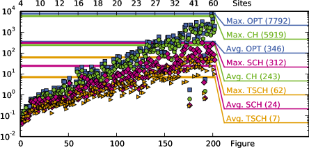
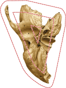
Quality. To analyze the quality of the labelings constructed by CH, SCH and TSCH, we compare the cost ratio $c(\mathcal{L}_{A})/c(\mathcal{L}_{\textsc{OPT}})$, where $\mathcal{L}_{\textsc{OPT}}$ is created by OPT and $\mathcal{L}_{A}$ is created by the variant $A\in\{\textsc{CH},\textsc{SCH},\textsc{TSCH}\}$; see Fig. 12. About $73\%$ (CH), $56\%$ (SCH) and $53\%$ (TSCH) of the labelings achieve optimal costs. For $90\%$ of the figures, the algorithms achieve labelings whose costs are at most a factor of $1.06$ (CH), $1.75$ (SCH) and $1.99$ (TSCH) worse than the optimal costs. Only for two figures no valid solution could be computed, because their contour was too small to host all labels; see Fig. 14. In particular, the bottom sides of the contours are almost horizontal, which means that too many labels must be placed along the left and right side of the contour. The designer of the original labeling avoided this problem by breaking design rule T5.

For the majority of the figures monotone labelings (criteria L4) were created. Only for one figure none of the algorithms could create a monotone labeling. For two further figures SCH and TSCH could not create monotone labelings, while the other two approaches did. Finally, for one figure only TSCH did not create a monotone figure.

A consulted domain expert stated that the created labelings would be highly useful as initial labeling for the remaining process of laying out the figure. According to the expert, the labelings already have high quality and would require only minor changes, due to aesthetic reasons. These can be hardly expressed as general criteria, but rely on the expertise of the designer. Altogether, the domain expert assessed our algorithm to be a tool of great use that could reduce the working load of a designer significantly.

Running Time. The average running times of our algorithms range between $7$ seconds (TSCH) and $346$ seconds (OPT); see Fig. 12. The variants SCH and TSCH are remarkably faster than OPT; see Fig. 12. On average they achieve a speedup by a factor of $8.4$ and $23.0$, respectively. For some figures, TSCH and SCH even achieve a speed up of $198$ and $76$. Further, TSCH and SCH never exceeded $62$ and $312$ seconds, respectively. On average TSCH is by a factor $2.5$ faster than SCH; in maximum by a factor of $7.1$. The variant CH only slightly improves OPT by a factor of $1.4$ on average and $3.7$ in maximum.

Since OPT has a high memory consumption, we ran the experiments on a server with 128 GB RAM. When such a system is not available, SCH and TSCH are appropriate alternatives for OPT, because they use significantly less memory, are fast and mostly produce labelings of high quality. To assess the applicability of the approaches in a typical setting, we ran both SCH and TSCH on an ordinary laptop with an Intel Core i7-3520M CPU clocked at $2.9$ GHz and $8$ GB of RAM. In comparison to the previous setting, SCH and TSCH are slower by a factor of $1.24$ and $1.22$ in maximum, respectively. On average SCH needs $28$ seconds and TSCH needs $8$ seconds. Within $27$ ($94$) minutes the labelings of all 202 figures were produced by TSCH (SCH); in contrast, a domain expert stated that creating a labeling for a figure with about $50$ sites by hand may easily take $30$ minutes.

Figure 14: Illustrations with original labelings. Due to the choice of the contour (red), both instances could not be solved by our approach. Source: Paulsen, Waschke, Sobotta Atlas Anatomie des Menschen, 23.Auflage 2010 ©Elsevier GmbH, Urban & Fischer, München.

8 Discussion

The evaluation shows that our approach computes high-quality labelings for the vast majority of instances in short time. While OPT and CH are mainly useful for evaluating our approach, SCH and TSCH are fast enough to be deployed in practice. If quality is more important than running time, SCH is preferable and otherwise TSCH Figure 11 shows an example where SCH yields a better result than TSCH, still in reasonable time.

Only for two illustrations we could not create any labelings due to the chosen contour. To avoid this problem one could incorporate more sophisticated procedures for creating the contour. However, we refrained from this, because we were mainly interested in evaluating the performance of our dynamic programming approach. Alternatively, the designer could appropriately adapt the contour in an interaction step.

Further, one can relax the convexity assumption in practice allowing more general contours. The cases when overlaps of text boxes may occur for non-convex contours are pathological. This further enhances the possibility to integrate interaction with the user, who could adapt the contour on demand. In most cases the running times of TSCH are sufficient for interactive editing, which is necessary for laying out professional books; for real-time scenarios (e.g., labeling images of ongoing surgeries) the performance of our approach needs further improvement. Identifying more rules for excluding unnecessary instances is one possibility to speed up the procedure.

Although the produced labelings already have high quality, we can improve on them by applying post-processing steps, e.g., fix the order of the labels and restart the dynamic programming approach on a larger set of ports to do fine-tuning on the label placement. More sophisticated post-processing steps are future work.

Similarly, for labeling the same image in different scales, one could, based on a large-scale master labeling, penalize changes in the radial ordering of the labels in other scales. Pre-computing the labelings for all given scales in that way, one minimizes layout changes between different zoom levels, which can be useful for interactive views. A detailed evaluation is also future work.

Finally, our approach supports a one-to-one correspondence between labels and sites. To also support multiple sites per label, one could create multiple leader candidates having different fork points. Excluding them mutually, this yields a simple adaption of our original approach. The main research questions is then to identify appropriate candidate positions for the fork points.

9 Conclusion

In this paper we presented a flexible model for contour labeling, which we validated through interviews with domain experts and a semi-automatic analysis on handmade labelings. With some engineering the developed dynamic programming approach can be used to generate labelings of high quality in short time. The presented approach is particularly interesting for creating labelings of large collections of figures that must follow the same design rules; a prominent example are figures in atlases of human anatomy.

In contrast to external labeling heuristics (e.g., [14, 2]), our full approach provides mathematically optimal, exact solutions. Moreover, we can use these optimal solutions to assess the performance of our faster heuristics quantitatively in terms of the cost ratio. Compared to other exact labeling algorithms (e.g. [6, 7]), our optimization model supports more general contours, non-uniform label shapes, and the flexible integration of additional soft and hard constraints.

References

- [1]
- [2] K. Ali, K. Hartmann, and T. Strothotte. Label layout for interactive 3D illustrations. J. WSCG, 13(1):1–8, 2005.
- [3] L. Barth, A. Gemsa, B. Niedermann, and M. Nöllenburg. On the Readability of Boundary Labeling. In Graph Drawing and Network Visualization (GD’15), volume 9411 of LNCS, pages 515–527. Springer, 2015.
- [4] M. A. Bekos, M. Kaufmann, M. Nöllenburg, and A. Symvonis. Boundary labeling with octilinear leaders. Algorithmica, 57(3):436–461, 2010.
- [5] M. A. Bekos, M. Kaufmann, K. Potika, and A. Symvonis. Area-feature boundary labeling. Computer Journal, 53(6):827–841, 2010.
- [6] M. A. Bekos, M. Kaufmann, A. Symvonis, and A. Wolff. Boundary labeling: Models and efficient algorithms for rectangular maps. Computational Geometry: Theory and Applications, 36(3):215–236, 2007.
- [7] M. Benkert, H. J. Haverkort, M. Kroll, and M. Nöllenburg. Algorithms for multi-criteria boundary labeling. J. Graph Algorithms and Applications, 13(3):289–317, 2009.
- [8] S. Bruckner and M. E. Gröller. Volumeshop: An interactive system for direct volume illustration. In Visualization (Vis’2005), page 85. IEEE, 2005.
- [9] M. Fink, J.-H. Haunert, A. Schulz, J. Spoerhase, and A. Wolff. Algorithms for labeling focus regions. IEEE Trans. Visualization and Computer Graphics, 18(12):2583–2592, 2012.
- [10] M. Fink and S. Suri. Boundary labeling with obstacles. In Canadian Conf. Computational Geometry (CCCG’16), pages 86–92, 2016.
- [11] G. Fuchs, M. Luboschik, K. Hartmann, K. Ali, H. Schumann, and T. Strothotte. Adaptive labeling for interactive mobile information systems. In Information Visualization (InfoVis’06), pages 453–459. IEEE, 2006.
- [12] A. Gemsa, J. Haunert, and M. Nöllenburg. Multirow boundary-labeling algorithms for panorama images. ACM Trans. Spatial Algorithms and Systems, 1(1):1–30, 2015.
- [13] T. Götzelmann, K. Hartmann, and T. Strothotte. Agent-based annotation of interactive 3d visualizations. In Smart Graphics (SG’06), volume 4073 of LNCS, pages 24–35. Springer, 2006.
- [14] K. Hartmann, K. Ali, and T. Strothotte. Floating labels: Applying dynamic potential fields for label layout. In Smart Graphics (SG’04), volume 3031 of LNCS, pages 101–113. Springer, 2004.
- [15] Z. Huang, S. Poon, and C. Lin. Boundary labeling with flexible label positions. In WALCOM: Algorithms and Computation (WALCOM’14), volume 8344 of LNCS, pages 44–55. Springer, 2014.
- [16] J. M. Keil, J. S. B. Mitchell, D. Pradhan, and M. Vatshelle. An algorithm for the maximum weight independent set problem on outerstring graphs. Computational Geometry: Theory and Applications, 2016. In press.
- [17] P. Kindermann, B. Niedermann, I. Rutter, M. Schaefer, A. Schulz, and A. Wolff. Multi-sided boundary labeling. Algorithmica, 76(1):225–258, 2016.
- [18] K. Mogalle, C. Tietjen, G. Soza, and B. Preim. Constrained labeling of 2d slice data for reading images in radiology. In Visual Computing for Biomedicine (VCBM’12), pages 131–138. Eurographics Assoc., 2012.
- [19] K. Mühler and B. Preim. Automatic textual annotation for surgical planning. In Vision, Modeling, and Visualization (VMV’09), pages 277–284. Eurographics Assoc., 2009.
- [20] M. Nöllenburg, V. Polishchuk, and M. Sysikaski. Dynamic one-sided boundary labeling. In Advances in Geographic Information Systems (ACM-GIS’10), pages 310–319. ACM, 2010.
- [21] F. Paulsen and J. Waschke. Sobotta Atlas of Human Anatomy, Vol. 3, 15th ed., English/Latin: Head, Neck and Neuroanatomy. Elsevier, 2013.
- [22] T. Stein and X. Décoret. Dynamic label placement for improved interactive exploration. In Non-Photorealistic Animation and Rendering (NPAR’08), pages 15–21. ACM, 2008.
- [23] M. Tatzgern, D. Kalkofen, R. Grasset, and D. Schmalstieg. Hedgehog labeling: View management techniques for external labels in 3D space. In Virtual Reality (VR’14), pages 27–32. IEEE, 2014.
- [24] M. Tatzgern, D. Kalkofen, and D. Schmalstieg. Dynamic compact visualizations for augmented reality. In Virtual Reality (VR’13), pages 3–6. IEEE, 2013.
- [25] I. Vollick, D. Vogel, M. Agrawala, and A. Hertzmann. Specifying label layout style by example. In User Interface Software and Technology (UIST’07), pages 221–230. ACM, 2007.
- [26] L. Čmolík and J. Bittner. Layout-aware optimization for interactive labeling of 3d models. Computers & Graphics, 34(4):378–387, 2010.