PHAST: Protein-like Heteropolymer Analysis by Statistical Thermodynamics

Abstract

PHAST is a software package written in standard Fortran, with MPI and CUDA extensions, able to efficiently perform parallel multicanonical Monte Carlo simulations of single or multiple heteropolymeric chains, as coarse-grained models for proteins. The outcome data can be straightforwardly analyzed within its microcanonical Statistical Thermodynamics module, which allows for computing the entropy, caloric curve, specific heat and free energies. As a case study, we investigate the aggregation of heteropolymers bioinspired on $A\beta_{25-33}$ fragments and their cross-seeding with $IAPP_{20-29}$ isoforms. Excellent parallel scaling is observed, even under numerically difficult first-order like phase transitions, which are properly described by the built-in fully reconfigurable force fields. Still, the package is free and open source, this shall motivate users to readily adapt it to specific purposes.

PROGRAM SUMMARY

Authors:

Rafael Bertolini Frigori

Program Title:

PHAST

Journal Reference:

Catalogue identifier:

Licensing provisions:

GNU/GPL version 3

Programming language:

FORTRAN 90, MPICH 3.0.4, CUDA 8.0

Computer:

PC

Operating system:

GNU/Linux (3.13.0-46), should also work on any Unix-based operational system.

Supplementary material:

Keywords:

Folding: thermodynamics, statistical mechanics, models, and pathways; Biopolymers, biopolymerization; Monte Carlo methods; Thermodynamics and statistical mechanics

PACS:

87.15.Cc; 82.35.Pq; 05.10.Ln; 64.70.qd

Classification:

External routines/libraries:

cuRAND (CUDA), Grace-5.1.22 or higher

Subprograms used:

Nature of the problem:

Nowadays powerful multicore processors (CPUs) and Graphical Processing Units (GPUs) became much popular and cost-effective, so enabling thermostatistical studies of complex molecular systems to be performed even in personal computers. PHAST provides not only an easily-reconfigurable parallel program for Monte Carlo simulations of linear heteropolymers, as coarse-grained models of proteins, but also permits the automatized microcanonical thermodynamic analysis of those systems.

Solution method:

PHAST has three main modules for complementary tasks as: to map any .pdb file-sequence to its inner lexicon by using a configurable hydrophobic scale, while the main simulational module performs parallel Monte Carlo simulations in the multicanonical (MUCA) ensemble and, the analysis module which extracts microcanonical observables from MUCA weights.

1 Introduction

Linear heteropolymeric chains of amino acids are known as polypeptides. Proteins, on the other hand, are a large class of biological polymers containing at least one long polypeptide. Together, they constitute a set of macromolecules performing a vast array of functions within organisms, whose specificities strongly depend on their detailed intramolecular interactions that leads to three-dimensional (native) structures by a folding mechanism. The thermodynamic hypothesis [1] states that the native structure of a protein is a unique, stable and kinetically accessible minimum of the free energy solely determined by its (primary) sequence of amino acids. However, eventual misfolding may produce dysfunctional proteins, so inducing the formation of cytotoxic amyloid aggregates, which can culminate on degenerative diseases as type 2 Diabetes Mellitus (DM2) [2] or Alzheimer (AD) [3].

Once those biopolymers are typical representatives of the so-called small-systems, where in general the equivalence of statistical ensembles does not hold (see [4] and references therein), the direct computation of their density of states is a well suited investigation method to result on the system microcanonical thermodynamics [5]. Nevertheless, performing such calculations at a high enough accuracy implies on accumulating large amounts of statistical data through Monte Carlo methods, as Wang-Landau [6] or the multicanonical (MUCA) ensemble [7]. Thus, it consists of a huge computational challenge, which can be reasonably alleviated just by conjugating efficient parallel algorithms and coarse-grained molecular force fields.

To accomplish these demands we designed PHAST, a simple and easy-to-use open source package that enables users to simulate and analyze the microcanonical thermostatistics of general models for semi-flexible linear polymers [8, 9], as coarse-grained proteins [10, 11, 12, 13]. The program brings fully reconfigurable built-in force fields that can be readily modified and extended, this makes it specially apt for prototyping of many-body interacting systems, as polymers embedded in crowded solutions [14]. It is written in standard Fortran and possess MPI and CUDA extensions [15, 16], so being able to efficiently run on most modern parallel computer architectures. The distribution is forbidden for commercial or military purposes, but we hope that PHAST is useful and could be eventually incorporated in other programs, while we kindly request to be informed accordingly. Still, it is naturally supposed to be acknowledged in all resulting publications.

The article is organized as follows, in the Section 2 we review some simulation background, this includes coarse-grained modelling and the derivation of microcanonical thermostatistics from parallel multicanonical simulations. The Section 3 encompasses an in-dept overview of application modules. In the Section 4 two concrete case studies involving heteropolymers bioinspired on amyloidogenic proteins are presented, so the aggregation of $A\beta_{25-33}$ fragments and their further cross-seeding with $IAPP_{20-29}$ isoforms are investigated in the context of a minimal coarse-grained model. The parallel scaling of such simulations is rigorously addressed, while their physical significance is outlined, when possible, by comparisons to other results from the literature. The Section 5 brings our conclusions and perspectives for further developments.

2 Simulation background

2.1 Modelling proteins and polymers

Coarse-graining is a widely employed modelling strategy to reduce the degrees of freedom of many-body macromolecular systems as heteropolymers [9, 17]. Moreover, the study of protein folding and aggregation, specially in crowded media [18], has also largely benefited from such approach [17]. In this vein, PHAST incorporates a configurable force field able to describe semi-flexible linear heteropolymers [8, 19, 20, 21] and general properties of protein-like structural phase transitions [10, 11, 12, 13]. In the present model, a primary sequence is translated to a simpler one according to a predefined rule (i.e. sorting each residue by its hydrophobic character), so the amino acids on a proteic backbone are mapped to a coarser chain of pseudo-atoms (beads).

Once original molecular interactions are mapped into simpler ones, non-bonded interactions among beads are represented through effective hydrophobic forces [22], as given by a Lennard-Jones potential $\left(LJ\right)$. Thus, it is natural to adopt a specific hydrophobic scale [23] to perform the aforesaid sequence translation, see Figure 1. By considering that hydrophobic residues $\left(A\right)$ form more strongly-interactive cores than hydrophilic ones $\left(B\right),$ the coupling constant for pairs of nonadjacent beads $\left(\sigma_{i},\sigma_{j}\right)$ may be defined by

$$C_{LJ}\left(\sigma_{i},\sigma_{j}\right)=\left\{\begin{array}[]{cc}+1&\sigma_{i}=\sigma_{j}=A\\ +\nicefrac{{1}}{{2}}&\sigma_{i}=\sigma_{j}=B\\ -\nicefrac{{1}}{{2}}&\sigma_{i}\neq\sigma_{j}\end{array}\right.$$ (1)

Notwithstanding the fact that the protein backbones are rather stiff, they may be well modelled as bead-spring heteropolymers. Therefore, the bounds between successive beads located at a distance $r_{l,l+1}$ are described by the usual finitely extensible nonlinear elastic potential (FENE) [24], while a bending potential term between three successive beads is considered as proportional to $\left(1-\cos\theta_{k}\right).$ The resulting energy for a single chain composed by $N$ beads may be written as

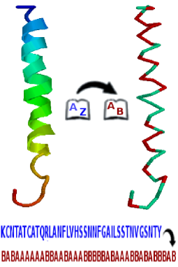
Figure 1: A chosen hydrophobicity scale is employed to map the FASTA sequence (A–Z) of a protein (on the left) extracted from the Protein Data Bank to another sequence, expressed by a two-letter code (A–B), which is ultimately used to build the coarse-grained one-bead protein model (on the right).

$$\begin{array}[]{c}H_{single}=\kappa_{F}R^{2}\sum_{l=1}^{N-1}C_{F}\left(\sigma_{l},\sigma_{l+1}\right)\ln\left(1-\left[\left(r_{l,l+1}-r_{0}\right)/R\right]^{2}\right)+\\ \\ \kappa_{C}\sum_{k=1}^{N-2}\left(1-\cos\theta_{k}\right)+\kappa_{LJ_{INTRA}}\sum_{i=1}^{N-2}\sum_{j=1+1}^{N}\left[r_{ij}^{-12}-C_{LJ}\left(\sigma_{i},\sigma_{j}\right)r_{ij}^{-6}\right],\end{array}$$ (2)

where the first term (FENE potential) has $\kappa_{F},$ $r_{0}$ and $R$ as general coupling constants for homopolymers, while $C_{F}\left(\sigma_{l},\sigma_{l+1}\right)$ allows for introducing different spring stiffness for heteropolymers. Moreover, $\kappa_{C}$ sets the chain rigidity against bends by an angle $\theta_{k},$ while $\kappa_{LJ_{INTRA}}$ defines the coupling constant of the non-bonded intramolecular $LJ$ potential between pairs of beads $\left(i,j\right)$ at a distance $r_{ij}$.

Finally, $M$ different chains are made to constitute a many-body interacting system by the following multi-chain potential

$$H_{multi}=\sum_{k=1}^{M}\left(H_{single,k}+\sum_{l>k}\sum_{i,j=1}^{N}\kappa_{LJ_{INTER}}\left[r_{l_{i}k_{j}}^{-12}-C_{LJ}\left(\sigma_{l_{i}},\sigma_{k_{j}}\right)r_{l_{i}k_{j}}^{-6}\right]\right),$$ (3)

where $H_{single,k}$ is given by Eq.(2), and the second term describes the non-bonded intermolecular $LJ$ potential between pairs of beads $\left(l_{i},k_{j}\right)$ at a distance $r_{l_{i}k_{j}},$ whose coupling constant is $\kappa_{LJ_{INTER}}.$

2.2 Parallel multicanonical simulations

It has been shown that microcanonical analysis of Monte Carlo simulations provide a powerful tool not only to precisely characterize structural phase transitions on small-systems [5, 8], where ensemble equivalence does not hold (see [4], and references therein), but also allows for neatly distinguish between good and bad folders among protein-like heteropolymers [25]. Most of straightforward implementations of such methodology rely on the accurate determination of systems density of states $\Omega\left(E\right),$ which may be achieved by the Wang-Landau method [6], or with generalized ensembles as the multicanonical [7].

Once knowing $\Omega\left(E\right),$ the microcanonical thermostatistics can be established by the usual Boltzmann formula for the entropy $S\left(E\right),$ as follows

$$S\left(E\right)=k_{B}\ln\Omega\left(E\right).$$ (4)

This leads to the microcanonical connection to thermodynamical observables [5]. For instance, numerical derivatives of the entropy $S\left(E\right)$ can be taken to compute quantities of interest, as the microcanonical caloric curve, relating the temperature $T$ to the internal energy $E,$ given by

$$\,k_{B}\beta\left(E\right)\equiv T\left(E\right)^{-1}=\frac{\partial S}{\partial E}.$$ (5)

Also, the microcanonical specific heat $C_{V}\left(E\right)$ is expressed as

$$C_{V}\left(E\right)=\frac{dE}{dT}=-\left(\frac{\partial S}{\partial E}\right)^{2}\left(\frac{\partial^{2}S}{\partial E^{2}}\right)^{-1},$$ (6)

while the free energy $F\left(E\right),$ at a fixed temperature $T_{c},$ is computed by

$$F\left(E\right)=E-\left.\left(\frac{\partial S}{\partial E}\right)^{-1}\right|_{E=E\left(T_{c}\right)}S\left(E\right).$$ (7)

As previously stated, the multicanonical ensemble offers a quite practical method to estimate $\Omega\left(E\right)$ through Monte Carlo simulations, and so, to obtain the microcanonical thermostatistics of any physical system. Basically, on this approach the entropy is written as a piecewise function of the discretized energies $E_{k}$ and a set of MUCA coefficients $\left\{\beta_{k},\alpha_{k}\right\},$ as follows

$$S_{muca}(E_{k})=\beta_{k}E_{k}\text{\textminus}\alpha_{k}.$$ (8)

The Monte Carlo simulations in the multicanonical ensemble naturally employ the so-called generalized MUCA weights $\,\omega_{muca}\left(E_{k}\right)\propto e^{-\beta_{k}E_{k}+\alpha_{k}}$, instead of the usual Boltzmann weights $\,\omega_{B}\propto e^{-\beta E}$, which enhances energetic tunnelings by improving the sampling of rare configurations.

However, those MUCA coefficients $\left\{\beta_{k},\alpha_{k}\right\}$ are a priori unknowns, so requiring an algorithm for their determination before a production run can be pursued. A successful technique to estimate MUCA weights is iterative [7] and involves computing histograms $H_{muca}\left(E\right)$ of the energies $E_{k}\in\left[E_{0},\ldots,E_{max}\right].$ Thus, in the beginning, one sets $\omega_{muca}^{0}(E_{k})=1$ for all energies $E_{k}$, which is used on an usual METROPOLIS simulation to collect the initial $\left(n=0\right)$ histogram $H_{muca}^{0}\left(E\right).$ Thereafter, it is applied a recursive update scheme for the MUCA weights $\omega_{muca}^{n+1}\left(E\right)=\omega_{muca}^{n}\left(E\right)/H_{muca}^{n}\left(E\right),$ before starting a new simulation with the lately estimated weights. This process is repeated till convergence is detected by a flatness check on the histograms. In the end, at a large-$n$ limit, the multicanonical entropy is ensured to recover the microcanonical one as $S_{muca}\left(E\right)\rightarrow S\left(E\right)$.

The multicanonical implementation on PHAST employs accumulated error-weighted histograms, so statistics for weight estimations improves for every repetition, while convergence is attained by Berg’s weight recursion[7]. Additionally, its parallel estimator for MUCA weights — initially proposed by Zierenberg et. al. [26] to study spin-systems — present scaling properties computationally exceeding more traditional approaches [27]. This is due to a simple and quite efficient update scheme, illustrated on Figure 2. First, each processor (node) is initialized with the same MUCA coefficients, but a particular random seed, then they perform independent Markov Chain Monte Carlo (MCMC) simulations to accumulate local energy histograms. After one iteration cycle those histograms are combined on the master node, which updates and then broadcasts the new MUCA weights, the cycle is repeated till convergence is achieved.

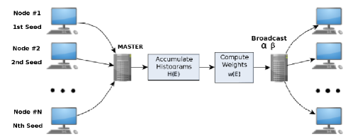
Figure 2: The iteration-cycle scheme for parallel multicanonical simulation: N processors (nodes) are initialized with different random seeds and so, evolve independent Markov Chains whose individual Histograms are accumulated on $H\left(E\right)$ at each MUCA iteration to update the weight $W\left(E\right).$ The resulting coefficients $\left(\alpha,\beta\right)$ on MUCA weights are then broadcasted.

3 Software framework

The PHAST package is constituted by the following modules

• SET_INPUT: prepares input protein sequences from PDB files

• PHAST: the main engine to run parallel multicanonical simulations

• ANALYST: computes the microcanonical thermostatistics from MUCA simulations

It is not possible to give here a highly detailed description of all program routines. Instead, we address the main features and data workflows of aforementioned modules in the following subsections, which afterwards is illustrated by some concrete study cases.

3.1 SET_INPUT

A single text file named ProteinSequences.txt is to be provided as input to the simulation module. But while users may manually encode each of its line entries, so describing protein (or polymeric) sequences according to an AB-like lexicon (e.g. Eq. 1), this can be alternatively generated in a quicker manner. To this end, the SET_INPUT module was designed to facilitate the mapping of protein structures, downloaded from the Protein Data Bank (PDB) [28], by using a built-in hidrophobicity scale [23] configured on file hscale.h.

The aforesaid mapping is attained by invoking the setup module (./set_input.o) and then typing the path to a (.pdb or .seq) input file, whereas the software shall recognize among valid PDB (.pdb) or three-letter code (.seq) sequences. Still, by successively calling this module with different file sequences, more lines are appended to ProteinSequences.txt, so making it quite easy to prepare input files even for simulations of multiple-proteic systems.

3.2 PHAST

This is the main module of the package, here multicanonical algorithms are implemented to simulate the coarse-grained models of Section 2. In principle, PHAST just needs to read a ProteinSequences.txt text file before starting any run. However, the software can be fully reconfigured (before compilation) through editing its .h files, whose content is

• vars.h: the main configuration file that sets multicanonical parameters. This includes, but is not limited to, the quantity and size of energy binnings, the number of MCMC sweeps and MUCA iterations, the definition of common blocks, the maximal size and number of proteins as well as of the residue families allowed in a simulation.

• set_hamiltonian.h: enables to tune the coupling constants specifying a particular Hamiltonian from Eq.(2) and Eq.(3).

• box_size.h: defines the size of the steric spherical container for proteins and some geometric cutoffs of polymer backbones.

• set_randvec_size.h: random numbers may be optionally generated as large vectors in GPUs, the size can be optimally adjusted to fit memory caches.

Still, the main module is composed by the following briefly summarized routines

• MAIN.F: is the principal routine of the simulation module, contains all MPI communication structures and callings of I/O and MUCA engine functions.

• HAMILTONIAN.f: given a polymeric configuration this routine computes the Hamiltonian defined by Eq.(2) and Eq.(3) with the constants adjusted at set_hamiltonian.h.

• MONTE_CARLO.f: this is a wrap routine that employs the Metropolis algorithm, with generalized MUCA weights, to perform MCMC stochastic evolutions. Additionally, it updates the local energy histograms at every simulation step.

• GEOMETRY.f: the simulation code uses inner coordinates, as bond-lengths and angles between beads, to evolve individual chains. This routine allows to convert them to (external) cartesian coordinates for computing inter-chain distances.

• UPDATE_ENGINE.f: this function stochastically updates all bead-positions of the chains contained in the 3d-spherical box defined at box_size.h. It employs a mix of optimized updating algorithms, to know, spherical-caps: that changes internal angles of each monomer along the backbone, pivotings: rotates a chain over a pivot direction, bond-length changes: by dilations or shrinks around the equilibrium value $r_{0}$ (if $\kappa_{F}\neq 0$), and Galilean-group updates: i.e. rotations plus translations of chains around the box center of mass. More details on references in [13].

• SET_HF-MATRIX.f: this routine permits to manually set the interaction coefficients $C_{LJ}\left(\sigma_{i},\sigma_{j}\right)$ and $C_{F}\left(\sigma_{i},\sigma_{j}\right)$ of the Hamiltonian in Eq.(2). It shall be modified accordingly to hscale.h, which allows for consistent generalizations of the AB-model lexicon such as [29].

• SET_MUCA.f: a bundle of auxiliary functions needed to set MUCA simulations.

• SET_PROT-SEQ.f: reads in proteins from the AB-sequence file ProteinSequences.txt.

• SET-SAVE_SIM.f: reads or writes to disk the simulation files, as protein configurations aAcidPosRxyz_*.pdb with extremal energies, produced during MCMC evolutions.

• SIM_IO-FILES.f: reads or writes to disk the inner control files of the simulation.

• RANDOM.f: the wrap function for random number generation on CPUs or GPUs.

• cudaRandom.cu: enables random number generation on GPUs.

It also shall be noted that as long as the simulations progress a serie of output files is automatically saved to disk. While files as Protein3DPositions.*, aAcid3DPositions.* and last.con are just intended for inner control of simulations, being specially needed when restarting simulations, there are also many other output files with *.dat or *.pdb extensions. As an example beta_n.dat, alpha_n.dat, g_n.dat, and hist_n.dat respectively denote files containing data from the n-th MUCA repetition, as the coefficients $\left\{\beta_{k},\alpha_{k}\right\}_{n}$, the density of states $g_{n}\left(E_{k}\right)$ and histograms $H_{n}\left(E_{k}\right)$ — which are read by the ANALYST module afterwards — as well as the aforementioned aAcidPosRxyz_*.pdb files.

3.3 ANALYST

This module is the kernel of the package for microcanonical thermostatistical analysis. A set of files, originally saved by the simulation module — i.e. beta_*.dat, alpha_*.dat, and last.con — is read and semi-automatically processed. As an outcome neat xmGrace [30] files are produced according to template files, named as template_*.agr. Some internal parameters shall be set before compilation, depending on the intended output features, to know

• icontrol: set intensive units of energy, as “energy per volume”, on the outputs.

• iAGR: defines if the thermodynamical observables of Eqs.(4)–(7) are written to individual .agr files, or combined into a single graph otherwise.

• Tol_Beta & Tol_L: respectively set (i) the numerical tolerance among three successive $\beta$ values and (ii) the minimal latent heat to be searched for during a Maxwell construction [5] on $\beta\left(\varepsilon\right)\times\varepsilon$.

In particular, when the ANALYST module is called (./analyst.o) the last.con file is read and supplies the software with parameters (set at vars.h) used on that former MUCA simulation. Then, the user is offered the option to type the configuration-ranges of the iteration files to be analyzed. Finally, the following additional information is requested to

• “Enter the number of monomers”: necessary to output data as intensive quantities.

• “Enter the finite difference step-size, dE: [0.01,9.9]”: the energy step dE is used to compute the finite-difference derivatives taken on $S\left(E\right).$

• “Enter the $\beta$ value to compute Free Energy, or 0 for Maxwell construction”: during first-order like structural phase transitions, the S-bends appear on microcanonical caloric curves. So users may wish to provide a specific $\beta_{c}$ to compute the Eq.(7), or let the program find this pseudo-critical value by a Maxwell construction.

4 Example runs

As case studies we have investigated two proteic systems by using the AB-model limit [10] of the Hamiltonian Eq.(3). Such modelling does not allows for prediction of protein structures, but may provide an useful method to learn about some general thermodynamical mechanisms underlying biological structural phase transitions [12]. For instance, this idea was successfully employed to compute aggregation propensities of peptides [13].

a typical "set_hamiltonian.h" file
!-------------------------------------------------------------
! Hamiltonian Parameters
!-------------------------------------------------------------
! Set c_KF, c_KC, c_KLJ_intra or c_KLJ_inter to 0.0d0 to
! Shutdown any of that interactions
!-------------------------------------------------------------
! FENE parameters: c_KF*R^2*ln(1-[(r-r0)/R]^2)
!-------------------------------------------------------------
r0 = 1.00d0     ! Distance of equilibrium between beads
R  = 1.2d0      ! Scale parameter
c_KF = 0.0d0    ! FENE coupling constant
!-------------------------------------------------------------
! Curvature parameters: c_KC*(1-cos*(Phi))
!-------------------------------------------------------------
c_KC = 0.25d0     ! Curvature coupling constant
!-------------------------------------------------------------
! Non-bonded interaction parameters: c_KLJ*(1/R^12-sigma/R^6)
!-------------------------------------------------------------
c_KLJ_intra = 4.00d0   ! Intra-protein LJ coupling constant
c_KLJ_inter = 4.00d0   ! Inter-protein LJ coupling constant

Therefore, while keeping in mind the limitations of our coarse-grained approach, we choose some natural amyloidogenic protein sequences as inspiration to generate aggregation-prone heteropolymeric chains through their hydrophobic mappings. So, we first simulate the aggregation of highly amyloidogenic segments of the Amyloid $\beta$ protein, associated to the Alzheimer disease — i.e. the $A\beta_{25-33}$ segment, PDB:2LFM — a system also applied for assessing the parallel scaling (Speedup) of our code. Additionally, we have simulated the aggregation of an heterogeneous molecular system, composed by segments of $A\beta_{25-33}$ and Amylin isoforms (related to the type 2 Diabetes Mellitus, see [13]) — i.e. the human $hIAPP_{20-29}$ PDB:2KB8 and rat $rIAPP_{20-29}$ PDB:2KJ7 — to test for catalytic effects of crowding [31] and cross-seeding [32] on the onset of aggregation that induces such degenerative diseases.

4.1 Aggregation of $A\beta_{25-33}$ segments: parallel speedup

To simulate the aggregation of $A\beta_{25-33}$ segments, we initially downloaded the 2LFM file from PDB [28] and SET_INPUT converted it to an AB-sequence. This sequence was then duly cut, cloned and used to prepare an input file to simulate the molecular aggregation (dimerization), as can be checked in the next data sample

ProteinSequences.txt
BBBBBAAAB
BBBBBAAAB

The box-radius $\left(R\right)$ was set to $R=40$ for these simulations and, overall statistics collected by the multiple processors was fixed to $10^{6}$ MCMC sweeps per MUCA iterations ($1.2\times 10^{6}$ for 128 processors), in a total of $10^{3}$ repetitions.

Before performing the data analysis of the resulting MUCA coefficients $\left\{\beta_{k},\alpha_{k}\right\}_{n},$ it was necessary to ensure they had reasonably converged after some minimal number of MUCA iterations $\left(N_{conv.}\right).$ To do so, we inspected the flatness of energy histograms $H_{n}\left(E_{k}\right)$ in the the full range of MUCA iterations, i.e. $n\in[1,1000].$ As an adequacy criteria we imposed that the Coefficient of Variation $\left(\mathrm{c_{Var}}=\nicefrac{{\sigma_{H}}}{{\mu_{H}}}\right),$ defined as the ratio of the standard deviation $\left(\sigma_{H}\right)$ over the average value of a histogram $\left(\mu_{H}\right)$, should be smaller than $5\%$. Additionally, local peaks on any supposedly flat histogram were to be no larger than $20\%$ of its average value. Considering both such constraints, we found acceptable convergence (i.e. enough histogram flatness) was established for data in the iteration range $n\in\left[N_{conv.}>175,1000\right]$, see Figure 3.

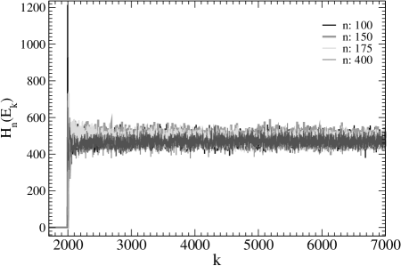
Figure 3: Representative energy histograms $H_{n}\left(E_{k}\right)$ employed for flatness checks, which also allows for identifying the convergence of MUCA coefficients $\left\{\beta_{k},\alpha_{k}\right\}_{n}$ during simulations of $A\beta_{25-33}$ segments. For histograms in the iteration range $n\in(175,1000]$ we observe acceptable Coefficient of Variation $\left(\mathrm{c_{Var}}\leq 5\%\right),$ see text.

Then, the ANALYST module was invoked to accomplish the thermostatistical data analysis. To ensure a robust estimation of the error bars, various starting $\left(N_{S}\geq N_{conv.}\right)$ and ending $\left(N_{E}\leq 1000\right)$ points in the iteration range $n\in\left[N_{S},N_{E}\right]$ of MUCA coefficients $\left\{\beta_{k},\alpha_{k}\right\}_{n}$ were tested, as well as the size of data-blocks $\triangle N$ (see Binning method, [33]) to be grouped in between. We also required the numerical stability and inter-compatibility (within the statistical errors) when computing the pseudo-critical inverse temperatures $\beta_{c},$ which was particularly important to improve the curve matchings during data collapses (Figure 4). Despite tedious, this procedure also enabled controlled checks of autocorrelation time effects over the statistical error bars.

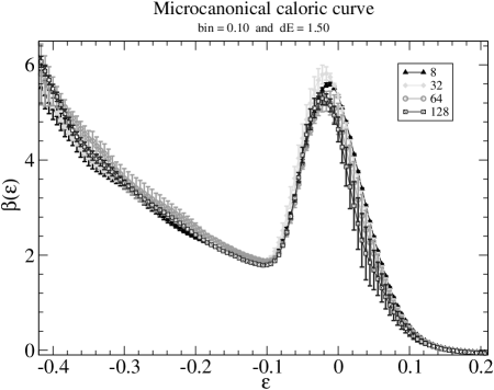
Figure 4: The data collapse of representative curves, of the inverse temperature $\beta\left(\varepsilon\right)\times\varepsilon,$ illustrates the equivalence on thermodynamical results from simulations employing up to 128 processors.

Figure 5: The microcanonical thermodynamic observables as seen from ANALYST module for the aggregation of $A\beta_{25-33}$ fragments, to know: the entropy $S\left(\varepsilon\right)\times\varepsilon$, caloric curve $\beta\left(\varepsilon\right)\times\varepsilon,$ the (shifted) free energy $f\left(=\varepsilon-\beta_{c}^{-1}\cdot S\right)\times\varepsilon,$ and specific heat $c_{v}\left(\varepsilon\right)\times\varepsilon.$

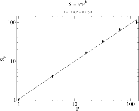
Figure 6: The parallel Speedup obtained for Multicanonical simulations present almost linear scaling up to hundred processors, even at numerically difficult first-order like phase transitions.

The physical consistency of our parallel results was validated by the data collapse of multiple simulations, performed with increasing number of CPUs (up to 128 processors) at the IBM P750 machine [34], see a representative output on Figure 4 for parameters $\left[N_{S},N_{E}\right]=\left[200,1000\right]$ and $\triangle N=50$. The general microcanonical behavior of the system was finally checked by an automatized plotting of the thermostatistical observables saved to an .agr file, as can be seen from Figure 5 (where $\left[N_{S},N_{E}\right]=\left[700,1000\right]$ and $\triangle N=25$). It is observed a first-order like structural phase transition, characterized by a reentrant on the microcanonical entropy $S\left(\varepsilon\right)$, which induces an S-bend on the caloric curve $\beta\times\varepsilon$ and also a region with negative values of the microcanonical specific heat $C_{v}\left(\varepsilon\right).$ See [5] for details and a comprehensive review on this formalism. It is also worth to note that such transitions are signaled by the presence of energetic barriers on the free energy, a feature we have previously studied on similar bioinspired molecular systems [12, 13].

To conclude, the wall times for simulations presenting equivalent thermodynamical results — which was ensured by performing a previous data collapse — were employed to analyze the parallel speedup of our code, seen on Figure 6. So we plotted the parallel Speedup factor $S_{p}=\nicefrac{{t_{1}}}{{t_{p}}},$ defined as the ratio of the serial $t_{1}$ to the parallel $t_{p}$ times spent to accomplish the convergence of MUCA weights. A power-law model $S_{p}=a\cdot P^{b}$ was proposed for regression, and so established an almost linear scaling $b=0.97\left(2\right)$ with the number of processors $P$. This corroborates the nice scaling properties of the parallel MUCA algorithm found on mild first-order like phase transitions [26, 35].

4.2 Cross-seeding of $A\beta_{25-33}$ and $IAPP{}_{20-29}$ isoforms

Recent clinical studies have suggested that DM2 can be a catalyst factor to the emergence of some neurodegenerative diseases, as the AD [36]. A microscopic molecular explanation, from in vitro studies [37], points to the cross-seeding of $A\beta$ and $IAPP$ as a key factor for the appearance of heterogeneous amyloid fibrils with considerable cytotoxicity. This phenomena would be somehow mimicked by the aggregation of bioinspired protein-like heteropolymers, investigated by the methodology previously applied to study the aggregation of $A\beta_{25-33}.$ Therefore, an input file was prepared by editing the AB-sequences obtained from SET_INPUT, once it is feed with the 2LFM ($A\beta$) and 2KB8 (hIAPP) files downloaded from PDB website [28]. That is

ProteinSequences.txt
BBBABAAABB
BBBABAAABB
BBBBBAAAB
BBBBBAAAB

also, an equivalent system for IAPP molecules of rats (PDB:2KJ7) was built, as shown

ProteinSequences.txt
BBBABAAAAA
BBBABAAAAA
BBBBBAAAB
BBBBBAAAB

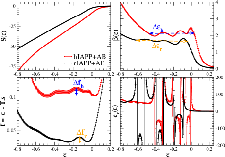
Figure 7: The microcanonical thermodynamic observables as seen from ANALYST module for the aggregation of $A\beta_{25-33}$ fragments cross-seeded by Amylin isoforms $hIAPP_{20-29}$ or $rIAPP_{20-29}$. To know: the entropy $S\left(\varepsilon\right)\times\varepsilon$, caloric curve $\beta\left(\varepsilon\right)\times\varepsilon$ including the Maxwell construction, the free energies $f\left(=\varepsilon-\beta_{c}^{-1}\cdot S\right)\times\varepsilon,$ and the specific heat $c_{v}\left(\varepsilon\right)\times\varepsilon.$ While the energetic barrier $\triangle f_{h}=0.034(5)$ for the aggregation of Human (h) molecular system is larger than the rodent (r) energetic barrier $\triangle f_{r}=0.021(3),$ its groundstate is found at much higher energies on the landscape. This explains the larger latent heats for the rodent system $\triangle\varepsilon_{r}=0.584\left(5\right)$ [to be compared to $\triangle\varepsilon_{h}=0.513\left(5\right)$], and so its increased stability against aggregation. The energy axis $\varepsilon=E/N$ is shown in intensive units.

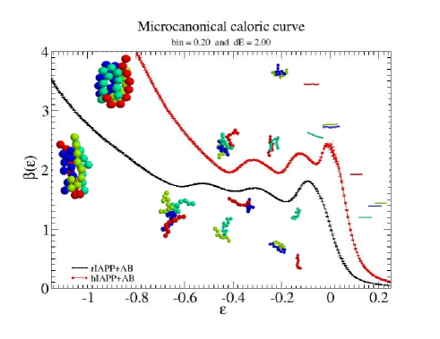
Figure 8: The microcanonical caloric curve $\beta\left(\varepsilon\right)\times\varepsilon$ with representative molecular configurations for the cross-seeding of fragments of $A\beta_{25-33}$ and Amylin isoforms: $hIAPP_{20-29}$ or $rIAPP_{20-29}.$

These simulations were run on a considerably denser environment, once the box-radius was set to $R=20.$ The 480 CPUs at [38] shared a workload of $10^{7}$ MCMC sweeps per MUCA iteration, in a total of $10^{3}$ MUCA repetitions. The obtained MUCA weights in the iteration range $\left[N_{S},N_{E}\right]=\left[700,1000\right]$ were analyzed with the ANALYST module, while taking $\triangle N=25$. Thermodynamical results are summarized for all microcanonical observables of both systems on Figure 7, while details for representative structures are exhibited on Figure 8. It is clearly observed that while the energetic barrier for the aggregation of the human molecular system (i.e. $A\beta_{25-33}$ and $hIAPP{}_{20-29}$) $\triangle f_{h}=0.034(5)$ is slightly larger than that of the rats system $\triangle f_{r}=0.021(3),$ the latter transition happens at much deeper values of the free energy. This fact justifies the larger latent heat found on the rodent system $\triangle\varepsilon_{r}=0.584\left(5\right)$ [to be compared to that of humans $\triangle\varepsilon_{h}=0.513\left(5\right)$], which explains thermodynamically its improved stability against aggregation.

Interesting enough, we also detected the presence of multiple backbendings on $\beta\left(\varepsilon\right)\times\varepsilon$ (see Figure 8), which are related to nucleation hierarchies, as broadly studied on [39]. Initially one observes the formation of one hetero-oligomer made of one segment of $A\beta_{25-33}$ and an Amylin isoform $(hIAPP_{20-29}$ or $rIAPP_{20-29}),$ whose thermodynamical signature emerges by the first bump on the caloric curves. Following, another hetero-oligomer is similarly built and, then finally the aggregation process is completed by a global collapse of both hetero-oligomers which results on a globular structure. It deserves to be noted that those aggregates are clearly not amyloidic ones, as no cross-beta structure is formed, which would require specific interactions for their stabilization a feature absent in our Hamiltonian. However, these protein-like aggregation transitions exhibit hierarchical nucleations as would also be expected by cooperative cross-seeding mechanisms on real proteins.

Therefore, some intriguing conclusions may be addressed from our microcanonical analysis, mainly regarding the stability of Amylin isoforms when cross-seeded by $A\beta$ segments. For example, a biotechnologically designed protein named Pramlintide [40] — originally inspired on PDB:2KJ7 — has been recently used as an adjuvant to treat DM2 in humans, curiously such protein becomes identical to $rIAPP$ when mapped by the hydrophobic scale [23] to the AB-model. Thus, our simulations indicate that Pramlintide could also be employed for damping the aggregation of heterogeneous amyloidogenic systems, as ones made by $A\beta$ and $IAPP$ isoforms. This result is corroborated not only by aggregation propensities previously computed from the AB-model [13], but also by studies of similar systems [31, 32] using all-atom force fields.

5 Conclusions

We have presented PHAST, a package for simulating coarse-grained models of proteins and bioinspired polymers in the multicanonical ensemble. Despite of its simple structure, the software comprises a reconfigurable force field which allows for an excellent parallel speedup. Additionally, its modules enable users to quickly map proteins downloaded from PDB to an inner AB-lexicon — or its generalizations as [29] — as well as to automatically compute most of systems microcanonical thermostatistics. Still, the program codes are open and free, which shall motivate students and researchers to readily adapt them to their specific purposes, as modelling many-body protein-protein interactions or the realistic effects of crowding on polymeric systems. We plan to gradually improve the built-in force fields, besides moving their calculations to GPUs, and implement faster evolution algorithms as hybrid MCMC [41].

References

- [1] C. B. Anfinsen, Science 181 4096 (1973) 223.
- [2] S. Melmed et al. Williams Textbook of Endocrinology (Elsevier/Saunders, Amsterdam, 2011); American Diabetes Society, http://www.diabetes.org/
- [3] A. Burns and S. Iliffe, BMJ 338:b158 (2009) 467.
- [4] N. A. Alves and R. B. Frigori, Phys. A 446 (2016) 195; R. B. Frigori, L. G. Rizzi , and N.A. Alves, Eur. Phys. J. B 75 (2010) 311.
- [5] D. H. E. Gross, Microcanonical Thermodynamics (World Scientific, Singapore, 2001).
- [6] F. Wang and D. P. Landau, Phys. Rev. Lett. 86 (2001) 2050; Phys. Rev. E 64 (2001) 056101; Comput. Phys. Commun. 147 (2002) 570.
-
[7]
B. A. Berg and T. Neuhaus, Phys. Lett. B 267 (1991)
249;
B. A. Berg, J. Stat. Phys. 82 (1996) 323;
B. A. Berg, Fields Inst. Commun. 26:1 (2000), arXiv:cond- mat/9909236;
B. A. Berg, Comput. Phys. Commun. 153 (2003) 397. - [8] S. Schnabel, D. T. Seaton, D. P. Landau, and M. Bachmann, Phys. Rev. E 84 (2011) 011127.
- [9] W. Janke and W. Paul, Soft Matter 12 (2016) 642.
-
[10]
F. H. Stillinger, T. Head-Gordon, and C. L. Hirshfeld,
Phys. Rev. E 48 (1993) 1469;
F. H. Stillinger and T. Head-Gordon, ibid. 52 (1995) 2872. - [11] C. Junghans, M. Bachmann, and W. Janke, Phys. Rev. Lett. 97 (2006) 218103.
- [12] R. B. Frigori, L. G. Rizzi, and N. A. Alves, J. Chem. Phys. 138 (2013) 015102.
- [13] R. B. Frigori, Phys. Rev. E 90 (2014) 052716.
-
[14]
R. J. Ellis, TRENDS in Bio. Sci.
26 (2001) 597;
I. M. Kuznetsova, K. K. Turoverov, and V. N. Uversky, Int. J. Mol. Sci. 15 (2014) 23090. - [15] http://mpi-forum.org/
- [16] https://developer.nvidia.com/cuda-zone
-
[17]
V. Tozzini, Curr. Opin. Struct.
Biol. 15 (2005) 144;
C. Wu and J.-E. Shea, ibid. 21 (2011) 209. -
[18]
A. Bille, B. Linse, S. Mohanty,
and A. Irbäck, J. Chem. Phys. 143 (2015) 175102;
S. Mittal, L. R. Singh, PlosONE 8 (2013) e78936;
D. Homouz, L. Stagg, P. Wittung-Stafshede, and M. S. Cheung, Biophys. J. 96 (2009) 671. - [19] J. Zierenberg, M. Mueller. P. Schierz, M. Marenz, and W. Janke, J. Chem. Phys. 141 (2014) 114908.
- [20] T. Chen, X. Lin, Y. Liu, T. Lu, and H. Liang, Phys. Rev E 78 (2008) 056101.
- [21] M. Bachmann, H. Arkın, and W. Janke, Phys. Rev. E 71 (2005) 031906.
- [22] D. Chandler, Nature (London) 437 (2005) 640.
- [23] M. A. Roseman, J. Mol. Biol. 200 (1988) 513.
- [24] R. B. Bird, C. F. Curtiss, R. C. Armstrong, and O. Hassager, Dynamics of Polymeric Liquids (Wiley, New York, 1987), 2nd ed.
- [25] J. Hernandez-Rojas, and J. M. Gomez Llorente, Phys. Rev, Lett. 100 (2008) 258104.
- [26] J. Zierenberg, M. Marenz, and W. Janke, Comput. Phys. Com. 184 (2013) 1155.
- [27] A. Mitsutake, Y. Sugita, and Y. Okamoto, J. Chem. Phys. 118 (2003) 6664.
- [28] http://www.rcsb.org/
- [29] S. Brown, N. J. Fawzi, and T. Head-Gordon, Proc. Natl. Acad. Sci. USA 100 (2003) 10712.
-
[30]
http://plasma-gate.weizmann.ac.il/Grace/
https://sourceforge.net/projects/qtgrace/ - [31] E. Rivera, J. Straub, and D. Thirumalai, Biophys. J. 96 (2009) 4552.
-
[32]
W. M. Berhanu, F. Yaşar,
and U. H. E. Hansmann, ACS Chem. Neurosci. 4 (2013) 1488;
W. M. Berhanu and U. H. E. Hansmann, PLoS ONE 9 (2014) e97051. - [33] B. A. Berg, Markov Chain Monte Carlo Simulations and Their Statistical Analysis (World Scientific, Singapore, 2004).
- [34] https://www.cenapad.unicamp.br/parque/IBM_div.shtml
- [35] J. Zierenberg, M. Marenz, and W. Janke, Phys. Proc. 53 (2014) 55.
- [36] Cheng, G., Huang, C., Deng, H., and Wang, H., Intern. Med. J. 42 (2012) 484.
- [37] Andreetto, E. et al., Angew. Chem., Int. Ed. 49 (2010) 3081; O’Nuallain, B. et al., J. Biol. Chem. 279 (2004) 17490.
- [38] http://sdumont.lncc.br/machine.php?pg=machine#
-
[39]
C. Junghans, W. Janke, and M. Bachmann,
Europhys. Lett. 87 (2009) 40002; Comp. Phys. Comm. 182 (2011) 1937.
T. Kocia and M. Bachmann, Physics Procedia 68 (2015) 80. - [40] P. A. Hollander et al., Diabetes Care 26 (2003) 784.
- [41] D. Simon, A. D. Kennedy, B. J. Pendleton, and D. Roweth, Phys. Lett. B. 195 (1987) 216.