Experimental demonstration of cheap and accurate phase estimation

Abstract

We demonstrate experimental implementation of robust phase estimation (RPE) to learn the phases of X and Y rotations on a trapped $\textrm{Yb}^{+}$ ion qubit. We estimate these phases with uncertainties less than $4\cdot 10^{-4}$ radians using as few as 176 total experimental samples per phase, and our estimates exhibit Heisenberg scaling. Unlike standard phase estimation protocols, RPE neither assumes perfect state preparation and measurement, nor requires access to ancillae. We cross-validate the results of RPE with the more resource-intensive protocol of gate set tomography.

I Introduction

As quantum computers grow in size, efficient and accurate methods for calibrating quantum operations are increasingly important Egger and Wilhelm (2014); Ferrie and Moussa (2015); Brown et al. (2011); Hou et al. (2016). Calibration involves estimating the values of experimentally tunable parameters of a quantum operation and, if incorrect, altering the controls to fix the error.

When these tunable parameters are incorrectly set, it causes the system to experience coherent errors. Coherent errors (versus incoherent errors) are more challenging for error correcting codes to correct Sanders et al. (2016); Gutiérrez et al. (2016), making it harder to reach fault-tolerant thresholds Kitaev (1997); Aharonov and Ben-Or (1997, 2008). Hence it is important to correct these types of errors in order to build a scalable quantum computer. While recent techniques using randomized compiling Wallman and Emerson (2016) mitigate the effects of coherent errors, removing as much of the coherent errors as possible still gives the best error rates.

Calibration can be challenging to perform without accurate state preparation and measurement (SPAM) estimates Stark (2014, 2015). Thus proper calibration of quantum operations will require robust protocols, that is, protocols that can accurately characterize gate parameters without highly accurate initial knowledge of SPAM.

A new technique for calibrating the phases of gate operations is robust phase estimation (RPE) Kimmel et al. (2015). RPE can be used to estimate the rotation axes and angles of single-qubit unitaries. Moreover, it is easy to implement (the sequences required are essentially Rabi/Ramsey experiments), simple and fast to analyze, and can obtain accurate estimates with surprisingly small amounts of data.

RPE has advantages over standard robust characterization procedures when it comes to the task of calibration. RPE can estimate specific parameters of coherent errors, whereas randomized benchmarking, while robust, can only estimate the magnitude of errors Knill et al. (2008); Magesan et al. (2012, 2011); Wallman et al. (2015); Sheldon et al. (2016). While compressed sensing approaches can withstand SPAM errors Shabani et al. (2011); Magesan et al. (2013), they do not have the Heisenberg scaling RPE achieves. There is a simple analytic bound on the size of SPAM errors that RPE can tolerate (namely less than $1/\sqrt{8}$ in trace distance), unlike the robust Bayesian approach of Wiebe et al., whose error tolerance is less well-understood. Wiebe et al. (2014). Lastly, RPE is extremely efficient compared to robust protocols that provide complete reconstructions of error maps, like randomized benchmarking tomography Kimmel et al. (2014) and gate set tomography (GST) Blume-Kohout et al. (2016).

Like many other phase estimation procedures, RPE achieves Heisenberg scaling Kimmel et al. (2015), but unlike many other protocols, requires no entanglement such as squeezed states or NOON states Caves (1981); Kitaev (1995); Kok et al. (2004); Giovannetti et al. (2006, 2004); Meyer et al. (2001); Lee et al. (2002), requires no ancillae Kitaev (1995); Boixo et al. (2007); Kessler et al. (2014), and is non-adaptive Wiseman (1995); Sergeevich et al. (2011); Higgins et al. (2007); Ferrie et al. (2013).

Finally, compared to many tomography and parameter estimation protocols, the post-experiment analysis of RPE is strikingly simple. There are no Bayesian updates Wiebe and Granade (2016); Ferrie et al. (2013); Wiebe et al. (2014), no optimizations Blume-Kohout et al. (2016); Svore et al. (2014); Shabani et al. (2011), and no fits to decaying exponentials Magesan et al. (2011); Kimmel et al. (2014). Instead, post-processing involves a dozen lines of pseudo-code, with the most complex operation being an arctangent (see Supplemental Material for more details).

Here, we provide the first published experimental demonstration of RPE and investigate its performance. We use RPE to experimentally extract the phases (rotation angles) of single-qubit unitaries. Because we don’t know the true values of the parameters, we benchmark these estimates by comparing to GST, which gives robust, accurate, and reliable estimates, but which requires much more data Blume-Kohout et al. (2016).

We see experimental evidence of Heisenberg scaling in RPE, and we attain an accuracy of $3.9\cdot 10^{-4}$ radians in our phase estimate using only 176 total samples. We compare these costs to GST and find that RPE requires orders of magnitude fewer total gates and samples to achieve similar accuracies. However, in regimes where experiments involving long sequences are not accessible, we find GST potentially has better performance than RPE. Nonetheless, due to its minimal data requirements, ease of implementation and analysis, and robust estimates of coherent errors, RPE is a powerful tool for efficient calibration of quantum operations.

II Preliminaries

We consider estimating the parameters $\alpha$ and $\epsilon$ from the single-qubit gate set Kimmel et al. (2015):

$$\hat{X}_{\pi/2+\alpha}= \exp\left[-i\left(\left(\pi/2+\alpha\right)/2\right)\hat{\sigma}_{X}\right],$$

$$\hat{Y}_{\pi/2+\epsilon}(\theta)= \exp\left[-i\left(\left(\pi/2+\epsilon\right)/2\right)\left(\cos\theta\hat{\sigma}_{Y}+\sin\theta\hat{\sigma}_{X}\right)\right],$$

where $\hat{\sigma}_{X}$ and $\hat{\sigma}_{Y}$ are Pauli operators, $\alpha$ and $\epsilon$ are rotation errors in the X and Y gates, respectively, and $\theta$ is the size of the off-axis component of the (ideally) Y gate rotation axis. There is no off-axis component to the X gates, as we choose the X axis of the Bloch sphere to be the rotation axis of the X gate. $\alpha$ and $\epsilon$ are parameters that experimentalists can typically control with ease.

In reality, the implemented gates will not be unitary, but instead will be completely positive trace preserving (CPTP) maps. Nonetheless, these CPTP maps will have rotation angles analogous to the angles $\alpha$ and $\epsilon$, and in the Supplemental Material, we show RPE can extract such angles. For the rest of the paper, with slight abuse of notation, we will use $\alpha$ and $\epsilon$ to refer to these more general CPTP map rotations.

We use both RPE and GST to extract $\alpha$ and $\epsilon$. Fig. 1 gives a schematic description of GST and RPE circuits. RPE circuits are essentially Rabi/Ramsey sequences; they consist of state preparation $\rho$, which for extracting $\alpha$ and $\epsilon$ is assumed to be not too far in trace distance from $|{0}\rangle\!\langle{0}|$, followed by repeated applications of the $X$ or $Y$ gate, followed by a measurement operator $M$, which is assumed to be close in trace distance to $|{1}\rangle\!\langle{1}|$. (Performing additional, more complex “Rabi/Ramsey-like” sequences allows for RPE to extract $\theta$ as well Kimmel et al. (2015); we do not do so here.)

RPE assumes all gates and SPAM are relatively close to ideal, but tolerates errors. We use “additive error” to denote the maximum bias in the outcome probability of any single RPE experimental sequence. This bias can be due to SPAM errors and incoherent errors in the gates. Additive error can be tolerated as long as it is less than $1/\sqrt{8}$.

For GST, each sequence consists of a state preparation $\rho$, followed by a gate sequence $F_{i}$ to simulate an alternate state preparation. Next a gate sequence $g_{k}$ is applied repeatedly. Finally, the measurement $M$ is preceded by a gate sequence $F_{j}$ to simulate an alternative measurement. We refer to $F_{i}$ and $F_{j}$ as state and measurement fiducials, respectively, and $g_{k}$ as a germ. (For more details, see the Supplemental Material.)

For both RPE and GST, running increasingly longer sequences produces increasingly accurate estimates. We use $L$ to parameterize the length of the sequence, as in Fig. 1. We run sequences with $L\in\{1,2,4,8,\dots,L_{\textrm{max}}\}$, where $L_{\textrm{max}}$ is chosen based on the desired accuracy. In RPE, we repeat the gate of interest either $L$ or $L+1$ times. In GST, we implement all possible combinations of state fiducials, measurement fiducials, and germs, with the germ repeated $\lfloor L/|g_{k}|\rfloor$ times, where $|g_{k}|$ is the number of gates in $g_{k}$ and $\lfloor\cdot\rfloor$ denotes the floor function.

We let $N$ be the repetitions (samples taken) of each sequence. We set $N$ to be the same for all sequences in a single RPE or GST experimental run. Although this results in slightly non-ideal scaling in the accuracy of our estimate Higgins et al. (2009), this is a realistic scenario for experimental implementation.

RPE successively restricts the possible range of the estimated phase using data from sequences with larger and larger $L$. Inaccuracies result when the procedure restricts to the wrong range. For larger values of $L_{\max}$, there are more rounds of restricting the range, and thus more opportunities for failure. By increasing $N$ when $L_{\max}$ increases, we can limit this probability of failure. Likewise, a large additive error makes it easier to incorrectly restrict the range, but again, taking larger $N$ can increase the probability of success. The interaction between accuracy, $N$, $L_{\max}$, and additive errors is shown in Fig. 2. This graph was created by adapting the analysis of Kimmel et al. (2015) to the case of fixed $N$ over the course of an RPE experimental run . Fig. 2 shows that, given an additive error $\delta$, there exist good choices for $N$ and $L_{\max}$, provided that $\delta<1/\sqrt{8}$.

A protocol has Heisenberg scaling when the root mean squared error (RMSE) of its estimate of a gate parameter scales inversely with the number of applications of a gate. RPE provably has Heisenberg scaling Kimmel et al. (2015), and GST numerically exhibits Heisenberg-like scaling Blume-Kohout et al. (2016). In this paper, we empirically look for scaling in accuracy and precision that scales as $1/L_{\textrm{max}}$. This is a good proxy (up to log factors) for Heisenberg scaling.

In practice, experimentalists care less about Heisenberg scaling, and more about the resources required to achieve a desired accuracy in their estimate. Therefore we are additionally interested in how large $N$ and $L_{\textrm{max}}$ should be to attain a desired precision. Assuming time is the key resource, if experimental reset time is long compared to gate time, $N$ becomes the dominant cost factor. On the other hand, if gate time is long compared to experimental reset time, $L_{\textrm{max}}$ is the dominant factor.

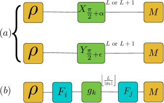
Figure 1: (Color online) (a) RPE and (b) GST experimental sequences. Each sequence starts with the state $\rho$ and ends with the two-outcome measurement $M$. (a) An RPE sequence consists of repeating the gate in question either $L$ or $L+1$ times. (b) In GST, a gate sequence $F_{i}$ is applied to simulate a state preparation potentially different from $\rho$. This is followed by $\lfloor L/|g_{k}|\rfloor$ applications of a germ—a short gate sequence $g_{k}$ of length $|g_{k}|$. Finally, a sequence $F_{j}$ is applied to simulate a measurement potentially different from $M$.

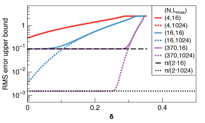
Figure 2: (Color online) Analytic upper bounds on the RMSE of the RPE phase estimate. Because RPE is potentially biased, the RMSE does not go to zero in the limit of infinite $N$, but instead, approaches a floor of $\pi/(2L_{\textrm{max}}).$ Larger additive error $\delta$ produces a larger bias, and thus require larger $N$ and larger $L_{\max}$ to achieve a small RMSE. For example, $N=16$ is not large enough to reach the floor for $L_{\max}=1024,$ but increasing $N$ to $370$ we easily saturate the bound for most values of $\delta$.

III Experimental results

Here we will give estimates of $\alpha$. Results for $\epsilon$ are similar and can be found in the Supplemental Material.

We implement GST and RPE on a single ¹⁷¹Yb⁺ ion in a linear surface ion trap. The qubit levels are the hyperfine clock states of the ${}^{2}S_{1/2}$ ground state: $|0\rangle=|F=0,m_{F}=0\rangle,|1\rangle=|F=1,m_{F}=0\rangle$. We initialize the qubit close to the $|0\rangle$ state via Doppler cooling and optical pumping; we measure in the computational basis (approximately) via fluorescence state detection Olmschenk et al. (2007). The desired operations are $X_{\pi/2}$ and $Y_{\pi/2}$. See Blume-Kohout et al. (2016) for experimental details. For the numerical analysis in this work, we have used the open-source GST software pyGSTi, and have extended its capabilities to include RPE functionality Nielsen et al. (2016).

We take 370 samples of each GST and RPE sequence. (For details, see Gate Sequences in Supplemental Material.) We use $L\in\{1,2,4,\dots,1024\}$. The GST dataset comprises 2,347 unique sequences and 868,390 total samples, while the RPE dataset comprises 44 sequences and 16,280 samples. The RPE dataset further disaggregate into disjoint sets of 22 unique sequences and 8,140 samples per phase.

Looking at Fig. 2, we see that $N=370$ is larger than necessary for RPE with $L_{\max}=1024$ for additive error less than $\sim 0.25$. To simulate experiments with fewer than 370 samples per sequence, we randomly sample (without replacement) from the experimental dataset, so that the new, subsampled dataset has $N<370$ samples per sequence.

We use several methods to characterize the experimental accuracy of RPE. First, we apply the analytic bounds on RMSE of Fig. 2. We also compare our subsampled RPE estimates to the GST estimate. Unlike RPE, GST is an unbiased estimator Blume-Kohout et al. (2013), so going to large $N$ (at a large cost in resources) gives standard quantum limit scaling. Using the $N=370$ dataset for GST, we estimate $\alpha-\pi/2=(6.4\pm 4.9)\cdot 10^{-5}$; the error bars denote a 95% confidence interval derived using a Hessian-based procedure (see Blume-Kohout et al. (2016) for details). On the other hand, using all RPE data we estimate $\alpha-\pi/2=1.0\cdot 10^{-4}$, with an RMSE upper bound of $\pi/(2\cdot L_{\max})\approx 1.5\times 10^{-3}$ (where this bound comes from Fig 2 with $N=370$, assuming our additive error is less than $0.25$; this assumption is borne out in the next section).

While the RPE estimate is consistent with the GST result, the accuracy is significantly lower, and we thus take $\alpha_{0}$, the full data estimate from GST, to be the “true” value of $\alpha$ for the purposes of benchmarking RPE. In particular, throughout this paper, we calculate experimental RMSE by comparing the mean estimate from 100 subsampled datasets to $\alpha_{0}$.

III.1 Heisenberg Scaling from RPE

To look for Heisenberg scaling in RPE estimates, we perform RPE on 100 subsampled datasets for $L_{\textrm{max}}\in\{1,2,4,\dots,1024\}$ with $N\in\{16,256\}$. We see Heisenberg-like scaling in the experimental RMSE in Fig. 3. We also plot $\pi/(2L_{\max})$, which is the analytic upper bound if sufficient samples are taken to compensate for additive error. We see that in practice, the analytic bounds can be pessimistic. Moreover, we see that while the experimental RPE accuracy is sensitive to $N$, increasing $N$ to $256$ from $16$ does not dramatically improve the RMSE, improving the scaling to $.078/L_{\max}$ from $.223/L_{\max}$. Instead, as expected, large increases in accuracy are obtained by moving to larger $L_{\max}$. This Heisenberg-like scaling is especially important for regimes where the time to implement the gate sequence is long relative to SPAM time.

We believe our experimentally derived bounds are significantly better than our analytic bounds in part because our system is well calibrated. The analytic bounds give a worst-case analysis that accounts for bias caused by adversarial additive error, but RPE is effectively unbiased for our system, up to the accuracy we achieve.

III.2 Comparison to GST

Because RPE can be biased, increasing $N$ cannot improve the RMSE below $\pi/(2L_{\max})$ in the worst case (see Fig. 2 and Kimmel et al. (2015)). However since GST is unbiased, it always benefits from increasing $N.$

We investigate this effect in Fig. 4. We plot the RMSE for experiments with fixed $L_{\max}=1024$, but $N\in\{8,16,\dots,256\}$. Analytic bounds for RPE are derived using the same method as in Fig 2. Experimental bounds for GST and RPE are derived from comparing the estimates of 100 subsampled datasets to $\alpha_{0}.$

While the analytic RPE bounds do not improve with increasing $N$, the subsampled RPE and GST datasets show standard quantum limit scaling. We expect this for GST, because GST is unbiased. In the case of RPE our experimental system happens to have very small additive error, and so is only very slightly biased. In this case, we expect to see improving estimates with increasing $N$ until our accuracy is about the same size as our bias. Fig. 4 tells us that for systems with relatively large additive error, where large $N$ is feasible but large $L_{\max}$ is not, GST can provide more accurate results.

However, we see in Fig. 4 that GST pays a substantial cost relative to RPE in required number of total samples (i.e., number of samples per sequence $N$ times total number of sequences). In Fig. 5, we compare the number of gates and samples which RPE and GST each require to achieve a desired accuracy, by analyzing 100 subsampled datasets with fixed $N=16$ and varying $L_{\max}\in\{1,2,4,\dots,1024\}.$ We see that RPE can achieve similar accuracy to GST while using at least an order of magnitude fewer total samples.

For our system, acquiring the entire RPE and GST datasets took 10.8 minutes and 12.1 hours, respectively, and total experimental time scales linearly with $N$. Thus we note that had our actual data acquisition rate been $N=16$, it would have taken 28 s to acquire that RPE dataset and about 31 minutes to acquire the GST dataset. As for analysis time, a single RPE dataset can be analyzed in about 0.05 s on a modern laptop. GST analysis takes about 20 s . All datasets and analysis notebooks are available online Rudinger et al. (2017).

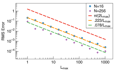
Figure 3: (Color online) RSME versus $L_{\max}$ for RPE estimates of $\alpha$ from 100 subsampled datasets of size $N=16$ and $N=256$. While analytic bounds are at best $\pi/(2L_{\max})$, we see this can be pessimistic. When the additive errors, which can bias the RPE estimate, are sufficiently small, increasing $N$ improves RMS accuracy.

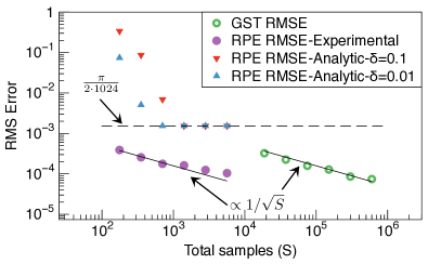
Figure 4: (Color online) Scaling of RMSE of estimates of $\alpha$ as a function of total samples (S), with $L_{\max}=1024$, and $N\in\{8,16,\dots,256\}$. The data point furthest left in each sequence corresponds to $N=8$, and the furthest right to $N=256.$ Analytic bounds are derived using the techniques of Fig 2. Experimental data points take the RMSE of 100 subsampled datasets for both RPE and GST. While the analytic bounds converge to $\pi/2048$, we see standard quantum limit scaling (i.e., error scaling $\propto 1/\sqrt{S}$) of RPE experimental estimates. As discussed in the text, this is because our experimental device has very low additive error, and thus the RPE estimates are essentially unbiased, and can achieve greater accuracy with increasing number of samples. GST estimates also exhibit standard quantum limit scaling.

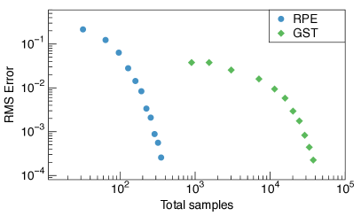
Figure 5: (Color online) RMSE for RPE and GST estimates of $\alpha$ versus total number of samples, using 100 subsampled datasets with $N=16$. Each sequential data point corresponds to setting $L_{\max}\in\{1,2,3,\dots,1024\}$. RPE achieves the same level of accuracy as GST using far fewer resources.

IV Conclusions

We show that robust phase estimation successfully estimates the phases of single-qubit gates, yielding results that are consistent with the full tomographic reconstruction of gate set tomography and also exhibits Heisenberg-like scaling in accuracy. In particular, an individual phase may be estimated with a root mean squared error of $3.9\cdot 10^{-4}$ with as few as 176 total samples.

Hence, RPE is a strong choice for diagnosing and calibrating single-qubit operations. It would be interesting to investigate whether the techniques of RPE can be applied to assessing other errors in single-qubit gate operations in a fast and accurate manner.

V Acknowledgements

Sandia National Laboratories is a multi-program laboratory managed and operated by Sandia Corporation, a wholly owned subsidiary of Lockheed Martin Corporation, for the U.S. Department of Energy’s National Nuclear Security Administration under contract DE-AC04- 94AL85000. SK is funded by the Department of Defense. The authors thank Robin Blume-Kohout and Nathan Wiebe for helpful conversations, and Erik Nielsen for extensive software support. This research was funded, in part, by the Office of the Director of National Intelligence (ODNI), Intelligence Advanced Research Projects Activity (IARPA). All statements of fact, opinion or conclusions contained herein are those of the authors and should not be construed as representing the official views or policies of IARPA, the ODNI, or the U.S. Government.

VI Supplemental Material

VI.1 Robust phase estimation on CPTP maps

In RPE, Kimmel et al. (2015), the gates to be analyzed are assumed to be close to some unitaries. Then RPE allows estimation of the error parameters of those unitaries (see Eq. 1). However, there is ambiguity in this formulation, because given a full description of completely positive and trace preserving (CPTP) map ${\mathcal{E}}$, there is not a unique unitary associated to this map. This might make it difficult to compare RPE and GST, since GST produces an estimate for a complete CPTP map. We now show that given a CPTP map ${\mathcal{E}}$ on a single qubit, RPE can extract the phase of the imaginary eigenvalues of that map.

We will use the Pauli-Liouville representation of CPTP maps, states and measurements (e.g. King and Ruskai (2001)). Let $P_{i}=\sigma_{i}$ (the single-qubit Pauli matrices) and let $P_{0}$ be the 2-by-2 identity matrix. Then for a single-qubit CPTP map ${\mathcal{E}}$, the Pauli-Liouville representation ${{\mathcal{E}}}^{P\!L}$ is given by

$${{\mathcal{E}}}^{P\!L}=\sum_{i,j=0}^{3}\frac{\operatorname{tr}\left({\mathcal{E}}(P_{i})P_{j}\right)}{2}|{i}\rangle\!\langle{j}|.$$ (1)

In the Pauli-Liouville representation, a single qubit density matrix $\rho$ is given by the vector $|{\rho}\rangle\!\rangle$ where

$$|{\rho}\rangle\!\rangle=\sum_{i=0}^{3}\frac{1}{\sqrt{2}}\operatorname{tr}(\rho P_{i})|i\rangle,$$ (2)

and a positive measurement operator $M$ is given by $\langle\!\langle{M}|$ where

$$\langle\!\langle{M}|=\sum_{i=0}^{3}\frac{1}{\sqrt{2}}\operatorname{tr}(MP_{i})\langle i|.$$ (3)

As a consequence of these definitions, we have that $\operatorname{tr}(M{\mathcal{E}}(\rho))=\langle\!\langle{M}|{{\mathcal{E}}}^{P\!L}|{\rho}\rangle\!\rangle.$ Thus, as in GST, using an invertible $4\times 4$ matrix $S$, we can transform all states $|{\rho}\rangle\!\rangle$, maps ${{\mathcal{E}}}^{P\!L}$, and measurements $\langle\!\langle{M}|$ as

$${{\mathcal{E}}}^{P\!L}\rightarrow S^{-1}{{\mathcal{E}}}^{P\!L}S$$

$$|{\rho}\rangle\!\rangle\rightarrow S^{-1}|{\rho}\rangle\!\rangle$$

$$\langle\!\langle{M}|\rightarrow \langle\!\langle{M}|S,$$ (4)

and not impact any observables.

For single-qubit CPTP maps, ${{\mathcal{E}}}^{P\!L}$ is a real $4\times 4$ matrix King and Ruskai (2001) with two real eigenvalues (one of which has value 1) and two complex eigenvalues (which are complex conjugates of each other, by the complex conjugate root theorem) . Let $re^{\pm i\phi}$ be the phases of the complex eigenvalues of a map ${{\mathcal{E}}}^{P\!L}$. Using a similarity transformation $S_{{\mathcal{E}}}$ (in particular, the matrix whose columns are the right eigenvectors of ${{\mathcal{E}}}^{P\!L}$), we can transform ${{\mathcal{E}}}^{P\!L}$ to ${{{\mathcal{E}}}^{P\!L}}^{\prime}=S_{{\mathcal{E}}}^{-1}{{\mathcal{E}}}^{P\!L}S_{{\mathcal{E}}}$, where ${{{\mathcal{E}}}^{P\!L}}^{\prime}$ has the form

$${{{\mathcal{E}}}^{P\!L}}^{\prime}=\left(\begin{array}[]{cccc}1&0&0&0\\ 0&re^{i\phi}&0&0\\ 0&0&re^{-i\phi}&0\\ 0&0&0&d\\ \end{array}\right).$$ (9)

Now suppose we can prepare the state ${\color[rgb]{0,0,0}\rho_{x}\approx|+\rangle\!\langle+|}$, and make measurements $M_{x}$ and $M_{y}$ (measurements in the $\sigma_{x}$ and $\sigma_{y}$ bases, respectively). By construction, we assert that, under the same similarity transformation $S_{{\mathcal{E}}}$, we have

$$S_{{\mathcal{E}}}^{-1}|{\rho_{x}}\rangle\!\rangle=(1/\sqrt{2},1/2,1/2,0)^{T}+|{\delta_{\rho_{x}}}\rangle\!\rangle$$

$$\langle\!\langle{M_{x}}|S_{{\mathcal{E}}}=(1/\sqrt{2},1/2,1/2,0)+\langle\!\langle{\delta_{M_{x}}}|$$

$$\langle\!\langle{M_{y}}|S_{{\mathcal{E}}}=(1/\sqrt{2},-i/2,i/2,0)+\langle\!\langle{\delta_{M_{y}}}|.$$ (10)

We may assert the above because any errors introduced by $S_{{\mathcal{E}}}$ get absorbed into the $\delta$ terms. (Physically $|{\delta_{\rho_{x}}}\rangle\!\rangle$, $\langle\!\langle{\delta_{M_{x}}}|$ and $\langle\!\langle{\delta_{M_{y}}}|$ correspond to additive errors present in the state preparation and measurement operations.) Then we have

$$\langle\!\langle{M_{x}}|({{\mathcal{E}}}^{P\!L})^{k}|{\rho_{x}}\rangle\!\rangle=\frac{1}{2}(1+\cos(k\phi))+\delta_{x}^{k}$$

$$\langle\!\langle{M_{y}}|({{\mathcal{E}}}^{P\!L})^{k}|{\rho_{x}}\rangle\!\rangle=\frac{1}{2}(1+\sin(k\phi))+\delta_{y}^{k}$$ (11)

where $({{\mathcal{E}}}^{P\!L})^{k}$ signifies acting with ${\mathcal{E}}$ repeatedly $k$ times, and $\delta_{x}^{k}$ and $\delta_{y}^{k}$ depend on $r$ as well as $|{\delta_{\rho_{x}}}\rangle\!\rangle$, $\langle\!\langle{\delta_{M_{x}}}|$, and $\langle\!\langle{\delta_{M_{y}}}|$.

Comparing Eq. VI.1 with Eq. (I.1)-(I.2) of Kimmel et al. (2015), we see that given these two types of measurements, RPE can be used to learn $\phi$, assuming $\delta^{k}_{x}$ and $\delta^{k}_{y}$ are not too large. Thus we can directly compare estimates of rotation angles obtained by GST or by RPE.

VI.2 Gate sequences

Detailed explanations for the choice of gate sequences used for RPE and GST are given in Kimmel et al. (2015) and Blume-Kohout et al. (2016), respectively. Here we simply provide complete descriptions of the gate sequences used.

Before proceeding further, we describe two notational conventions: We denote the $X_{\pi/2}$ gate as $G_{x}$, and $Y_{\pi/2}$ gate as $G_{y}$. Additionally, sequences are listed in operation order, not matrix multiplication order, so the sequence $G_{x}G_{y}$ means “apply the $X_{\pi/2}$ gate, and then apply the $Y_{\pi/2}$ gate”.

Both RPE and GST rely on gate sequences that have a well-defined structure. For GST, each sequence is of the following form:

1. Prepare a fixed input state.

2. Apply a short gate sequence (called a fiducial preparation, denoted $F_{i}$) to simulate a particular state preparation.

3. Apply a short gate sequence (called a germ, denoted $g_{k}$) $\lfloor L/|g_{k}|\rfloor$ times, where $|g_{k}|$ is the number of gates in the germ, and $L\in\mathbb{Z}^{+}$ is the sequence length.

4. Apply a short gate sequence (called a fiducial measurement, denoted $F_{j}$) to simulate a particular measurement operation.

5. Perform and record the outcome of a fixed measurement.

RPE uses fiducial sequences and germs as well. However, the fiducial sequences are not independent of the germ under consideration, as we will describe in more detail when we discuss the specific RPE gate sequences.

We divide experiments into generations, labeled by $m\in\{0,1,\dots\}.$ Sequences in generation $m$ have sequence length $L=2^{m}$. For example, for the $m=3$ generation, the underlying sequence (modulo fiducials) for the germ $G_{x}$ is simply $G_{x}^{8}$; for the germ $G_{x}G_{y}$, it is $(G_{x}G_{y})^{4}$, and for the germ $G_{y}G_{x}G_{y}G_{x}G_{x}G_{x}$, it is just $G_{y}G_{x}G_{y}G_{x}G_{x}G_{x}$.

In GST, for each generation and each germ, sequences are run with every possible pairing of fiducial state preparation and measurement. That is, if there are $f_{p}$ and $f_{m}$ unique fiducial preparations and measurements respectively, then there are $f_{p}\cdot f_{m}$ unique sequences for a particular germ for a particular generation.

In our experiments, there are 11 generations in total (ranging from $m=0$ to $m=10$). Additionally, our target preparation operation is always $|0\rangle\langle 0|$, and our target measurement operation is always $\sigma_{z}$.

VI.2.1 GST fiducials

The preparation and measurement fiducials that we use for GST are, conveniently, identical. They correspond to mapping both the state preparation and measurement vectors to the six antipodal points on the Bloch sphere that intersect with the X, Y, and Z axes. Therefore, each germ at each generation generates 36 different sequences. The fiducials are:

1. {} (The null sequence; do nothing for no time.)

2. $G_{x}$

3. $G_{y}$

4. $G_{x}G_{x}$

5. $G_{x}G_{x}G_{x}$

6. $G_{y}G_{y}G_{y}$

VI.2.2 GST germs

The germs we use for GST in this Letter are:

1. $G_{x}$

2. $G_{y}$

3. $G_{x}G_{y}$

4. $G_{y}G_{y}G_{y}G_{x}$

5. $G_{y}G_{x}G_{y}G_{x}G_{x}G_{x}$

6. $G_{y}G_{x}G_{y}G_{y}G_{x}G_{x}$

7. $G_{y}G_{y}G_{y}G_{x}G_{y}G_{x}$

8. $G_{x}G_{x}G_{y}G_{x}G_{y}G_{y}$

VI.2.3 RPE germs and fiducials

The fiducials and germs used in an RPE sequence will depend on both the quantity being estimated, and the native fixed input and fixed measurement. In particular, for our experimental system, we believe that the fixed input state is close to $|0\rangle\langle 0|$ and the fixed measurement is close $\sigma_{z}$. Then for $\alpha$ (the amount of over- or under-rotation in $G_{x}$), the germ is $G_{x}$, state preparation is always the empty fiducial $\{\}$, and there are two measurement fiducials, the empty fiducial $\{\}$ and the gate $G_{x}$; for $\epsilon$ (the amount of over- or under-rotation in $G_{y}$), the germ is $G_{y}$, state preparation is always the empty fiducial $\{\}$, and there are two measurement fiducials, the empty fiducial $\{\}$ and the gate $G_{y}$;

Therefore, every RPE sequence we apply has one of the following forms:

1. ${G_{x}}^{2^{m}}$

2. ${G_{x}}^{2^{m}+1}$

3. ${G_{y}}^{2^{m}}$

4. ${G_{y}}^{2^{m}+1}$

for $m\in\{0,\cdots,10\}$.

VI.3 RPE Algorithm

We use the following is the algorithm that takes raw data counts from a robust phase estimation experiment, and returns an estimate of the phase. An open-source implementation of this protocol is available online Nielsen et al. (2016).

Algorithm 1

1:

2:$\vec{M}\in[\mathbb{Z}^{+}]^{n}$, a vector whose $i\textsuperscript{th}$ element $M_{i}$ is the number of repetitions (samples) of the $i\textsuperscript{th}$ experiment.

3:$\vec{x}\in[\mathbb{Z}^{+}]^{n}$, a vector whose $i\textsuperscript{th}$ input $x_{i}$ is sampled from a binomial distribution $B(\cos(2^{i-1}\phi)/2+1/2+\delta_{i,x},M_{i})$, with $\delta_{i,x}\in[0,1]$ for all $i$.

4:$\vec{y}\in[\mathbb{Z}^{+}]^{n}$, a vector whose $i\textsuperscript{th}$ input $y_{i}$ is sampled from a binomial distribution $B(\sin(2^{i-1}\phi)/2+1/2+\delta_{i,y},M_{i})$, with $\delta_{i,y}\in[0,1]$ for all $i$.

5:Estimate $\hat{\phi}\in[-\pi,\pi]$ of $\phi$

6:function RobustPhaseEstimation($\vec{M}$, $\vec{x}$, $\vec{y}$)

7:     $\textrm{Estimate}=0$ $\triangleright$ Initial estimate could be any value in $[-\pi,\pi]$; algorithm would be unaffected.

8:     for $i=1$ to $n$ do

9:         $L=2^{i-1}$

10:         $\textrm{CurrentPhase}=\arctan 2((x_{i}-M_{i}/2)/M_{i},-(y_{i}-M_{i}/2)/M_{i}))/L$ $\triangleright$ Calculate the remainder of the estimate mod $1/L$.

11:         while $\textrm{CurrentPhase}<(\textrm{Estimate}-\pi/L)$ do

12:              $\textrm{CurrentPhase}=\textrm{CurrentPhase}+2\pi/L$ $\triangleright$ If smaller than allowed principle range, increase until in range.

13:         end while

14:         while $\textrm{CurrentPhase}>(\textrm{Estimate}+\pi/L)$ do

15:              $\textrm{CurrentPhase}=\textrm{CurrentPhase}-2\pi/L$ $\triangleright$ If larger than allowed principle range, decrease until in range.

16:         end while

17:         $\textrm{Estimate}=\textrm{CurrentPhase}$

18:     end for

19:     return Estimate

20:end function

VI.4 Results for $\epsilon$

We now present our experimental results for the rotation angle $\epsilon$, corresponding to Figs. 3 and 5. We see that the $\epsilon$ estimate and error bar behaviors are both qualitatively and quantitatively similar to the $\alpha$ behavior. In particular, we observe $1/L_{\max}$ scaling in the RPE estimates for $\epsilon$ at $N$ as low as 16, and the observed RMSE scaling constant is below that guaranteed by RPE theory. Additionally, we find that, using the full $N=370$ dataset, GST returns the estimate $\epsilon-\pi/2=2.7\cdot 10^{-5}\pm 3.5\cdot 10^{-5}$. RPE provides a consistent estimate of $\epsilon-\pi/2=9.9\cdot 10^{-5}$, with an RMSE upper bound of $\pi/(2\cdot L_{\max})\approx 1.5\times 10^{-3}$.

Figure 6: (Color online) Root mean squared error vs $L_{\max}$ for RPE estimates of the angle $\epsilon$ from subsampled datasets with $N=16$ and $N=256$. 100 subsampled datasets are used for each value of $N$. This plot is analogous to the plot shown in Fig. 3; for further details, see caption of that figure.

Figure 7: (Color online) Root mean squared error vs total number of samples for RPE and GST estimates of the angle $\epsilon$ from the subsampled datasets with $N=16$. This plot is analogous to the plot given in Fig. 5; for further details, see caption of that figure.

References

- Egger and Wilhelm (2014) D. J. Egger and F. K. Wilhelm, Phys. Rev. Lett. 112, 240503 (2014).
- Ferrie and Moussa (2015) C. Ferrie and O. Moussa, Phys. Rev. A 91, 052306 (2015).
- Brown et al. (2011) K. R. Brown, A. C. Wilson, Y. Colombe, C. Ospelkaus, A. M. Meier, E. Knill, D. Leibfried, and D. J. Wineland, Phys. Rev. A 84, 030303 (2011).
- Hou et al. (2016) Z. Hou, H.-S. Zhong, Y. Tian, D. Dong, B. Qi, L. Li, Y. Wang, F. Nori, G.-Y. Xiang, C.-F. Li, and G.-C. Guo, New Journal of Physics 18, 083036 (2016).
- Sanders et al. (2016) Y. R. Sanders, J. J. Wallman, and B. C. Sanders, New Journal of Physics 18, 012002 (2016).
- Gutiérrez et al. (2016) M. Gutiérrez, C. Smith, L. Lulushi, S. Janardan, and K. R. Brown, Phys. Rev. A 94, 042338 (2016).
- Kitaev (1997) A. Y. Kitaev, Russian Mathematical Surveys 52, 1191 (1997).
- Aharonov and Ben-Or (1997) D. Aharonov and M. Ben-Or, in Proceedings of the Twenty-ninth Annual ACM Symposium on Theory of Computing, STOC ’97 (ACM, New York, NY, USA, 1997) pp. 176–188.
- Aharonov and Ben-Or (2008) D. Aharonov and M. Ben-Or, SIAM Journal on Computing 38, 1207 (2008).
- Wallman and Emerson (2016) J. J. Wallman and J. Emerson, Phys. Rev. A 94, 052325 (2016).
- Stark (2014) C. Stark, Phys. Rev. A 89, 052109 (2014).
- Stark (2015) C. Stark, ArXiv e-prints (2015), arXiv:1510.02800 [quant-ph] .
- Kimmel et al. (2015) S. Kimmel, G. H. Low, and T. J. Yoder, Phys. Rev. A 92, 062315 (2015).
- Knill et al. (2008) E. Knill, D. Leibfried, R. Reichle, J. Britton, R. B. Blakestad, J. D. Jost, C. Langer, R. Ozeri, S. Seidelin, and D. J. Wineland, Phys. Rev. A 77, 012307 (2008).
- Magesan et al. (2012) E. Magesan, J. M. Gambetta, and J. Emerson, Phys. Rev. A 85, 042311 (2012).
- Magesan et al. (2011) E. Magesan, J. M. Gambetta, and J. Emerson, Phys. Rev. Lett. 106, 180504 (2011).
- Wallman et al. (2015) J. Wallman, C. Granade, R. Harper, and S. T. Flammia, New Journal of Physics 17, 113020 (2015).
- Sheldon et al. (2016) S. Sheldon, L. S. Bishop, E. Magesan, S. Filipp, J. M. Chow, and J. M. Gambetta, Phys. Rev. A 93, 012301 (2016).
- Shabani et al. (2011) A. Shabani, R. L. Kosut, M. Mohseni, H. Rabitz, M. A. Broome, M. P. Almeida, A. Fedrizzi, and A. G. White, Phys. Rev. Lett. 106, 100401 (2011).
- Magesan et al. (2013) E. Magesan, A. Cooper, and P. Cappellaro, Phys. Rev. A 88, 062109 (2013).
- Wiebe et al. (2014) N. Wiebe, C. Granade, C. Ferrie, and D. G. Cory, Phys. Rev. Lett. 112, 190501 (2014).
- Kimmel et al. (2014) S. Kimmel, M. P. da Silva, C. A. Ryan, B. R. Johnson, and T. Ohki, Phys. Rev. X 4, 011050 (2014).
- Blume-Kohout et al. (2016) R. Blume-Kohout, J. King Gamble, E. Nielsen, K. Rudinger, J. Mizrahi, K. Fortier, and P. Maunz, ArXiv e-prints (2016), arXiv:1605.07674 [quant-ph] .
- Caves (1981) C. M. Caves, Phys. Rev. D 23, 1693 (1981).
- Kitaev (1995) A. Y. Kitaev, eprint arXiv:quant-ph/9511026 (1995), quant-ph/9511026 .
- Kok et al. (2004) P. Kok, S. L. Braunstein, and J. P. Dowling, Journal of Optics B: Quantum and Semiclassical Optics 6, S811 (2004).
- Giovannetti et al. (2006) V. Giovannetti, S. Lloyd, and L. Maccone, Phys. Rev. Lett. 96, 010401 (2006).
- Giovannetti et al. (2004) V. Giovannetti, S. Lloyd, and L. Maccone, 306, 1330 (2004).
- Meyer et al. (2001) V. Meyer, M. A. Rowe, D. Kielpinski, C. A. Sackett, W. M. Itano, C. Monroe, and D. J. Wineland, Phys. Rev. Lett. 86, 5870 (2001).
- Lee et al. (2002) H. Lee, P. Kok, and J. P. Dowling, Journal of Modern Optics 49, 2325 (2002).
- Boixo et al. (2007) S. Boixo, S. T. Flammia, C. M. Caves, and J. M. Geremia, Phys. Rev. Lett. 98, 090401 (2007).
- Kessler et al. (2014) E. M. Kessler, I. Lovchinsky, A. O. Sushkov, and M. D. Lukin, Phys. Rev. Lett. 112, 150802 (2014).
- Wiseman (1995) H. M. Wiseman, Phys. Rev. Lett. 75, 4587 (1995).
- Sergeevich et al. (2011) A. Sergeevich, A. Chandran, J. Combes, S. D. Bartlett, and H. M. Wiseman, Phys. Rev. A 84, 052315 (2011).
- Higgins et al. (2007) B. L. Higgins, D. W. Berry, S. D. Bartlett, H. M. Wiseman, and G. J. Pryde, Nature 450, 393 (2007).
- Ferrie et al. (2013) C. Ferrie, C. E. Granade, and D. G. Cory, Quantum Information Processing 12, 611 (2013).
- Wiebe and Granade (2016) N. Wiebe and C. Granade, Phys. Rev. Lett. 117, 010503 (2016).
- Svore et al. (2014) K. M. Svore, M. B. Hastings, and M. Freedman, Quantum Info. Comput. 14, 306 (2014).
- Higgins et al. (2009) B. L. Higgins, D. W. Berry, S. D. Bartlett, M. W. Mitchell, H. M. Wiseman, and G. J. Pryde, New Journal of Physics 11, 073023 (2009).
- Olmschenk et al. (2007) S. Olmschenk, K. C. Younge, D. L. Moehring, D. N. Matsukevich, P. Maunz, and C. Monroe, Phys. Rev. A 76, 052314 (2007).
- Nielsen et al. (2016) E. Nielsen, K. Rudinger, J. K. Gamble IV, and R. Blume-Kohout, “A python implementation of gate set tomography,” (2016).
- Blume-Kohout et al. (2013) R. Blume-Kohout, J. King Gamble, E. Nielsen, J. Mizrahi, J. D. Sterk, and P. Maunz, ArXiv e-prints (2013), arXiv:1310.4492 [quant-ph] .
- Rudinger et al. (2017) K. Rudinger, S. Kimmel, D. Lobser, and P. Maunz, “https://github.com/pygstio/supplemental-info-rpe-1,” (2017).
- King and Ruskai (2001) C. King and M. B. Ruskai, IEEE Trans. Inf. Theor. 47, 192 (2001).