11institutetext: Czech Technical University in Prague, FNSPE, Břehová 7, 11519 Prague 1, Czech Republic 22institutetext: Comenius University, FMPI, Mlynská Dolina F1, 84248 Bratislava, Slovakia 33institutetext: Univerzita Mateja Bela, FPV, Tajovského 40, 97401 Banská Bystrica, Slovakia 44institutetext: Eötvös Loránd University, Pázmány P. s. 1/a, H-1117 Budapest, Hungary

Higher-order anisotropies in the Blast-Wave Model – disentangling flow and density field anisotropies

Jakub Cimerman 1122    Boris Tomášik 1133    Máté Csanád 44    and Sándor Lökös 44
Abstract

We formulate a generalisation of the blast-wave model which is suitable for the description of higher order azimuthal anisotropies of the hadron production. The model includes anisotropy in the density profile as well as an anisotropy in the transverse expansion velocity field. We then study how these two kinds of anisotropies influence the single-particle distributions and the correlation radii of two-particle correlation functions. Particularly we focus on the third-order anisotropy and consideration is given averaging over different orientations of the event plane.

pacs:
25.75.Dw, 25.75.Gz, 25.75.Ld

1 Introduction

The hot matter excited in ultrarelativistic heavy-ion collisions at colliders like the LHC or RHIC exhibits a sizeable anisotropy in particle production perpendicularly to the beam direction Abelev:2014pua ; ATLAS:2012at ; Chatrchyan:2012ta ; Abelev:2008ae ; Adler:2003kt . The azimuthal anisotropy of hadron momentum distributions, measured in terms of Fourier coefficients, is caused by the anisotropy of the fireball at freeze-out in spatial density and expansion pattern. That, in turn, results from its evolution which starts from anisotropic initial conditions Gale:2012rq ; Niemi:2012aj ; Floerchinger:2013hza ; Qian:2013nba ; Heinz:2013wva and may further receive anisotropic excitations on the way Schulc:2014jma ; Nahrgang:2011vn ; Tachibana:2017syd ; Crkovska:2016flo . The evolution depends on the Equation of State and the transport coefficients Luzum:2009sb ; Ryu:2015vwa ; Denicol:2015nhu . Thus by measuring the final state anisotropies one gets an access to the intrinsic properties of the matter Bernhard:2016tnd . Note that the anisotropies are unique in each event and a large fraction of them, especially higher-order anisotropies, are averaged out if measured in a sample consisting of a large number of events.

Hadrons are emitted at the moment of freeze-out and this is when their distributions are formed. Hence, the direct information that they are carrying is about the state of the fireball at this very moment. The present paper deals with this relation. It is then the task for hydrodynamic and/or transport simulations to conclude about the preceding evolution of the fireball.

There are two kinds of anisotropies of the fireball at the moment of freeze-out, that may cause an anisotropy of the hadron distribution Tomasik:2004bn ; Csanad:2008af ; Plumberg:2013nga ; Lokos:2016fze . Firstly, if the transverse expansion velocity in some directions is higher than in the others, the stronger blueshift of the momentum spectra in those directions will cause momentum anisotropy. Secondly, alone an expanding and spatially anisotropic fireball may also produce an anisotropy of the momentum distribution. Unfortunately, the two mechanisms cannot be distinguished by mere measurement of the momentum anisotropies.

For the second-order anisotropies it has been shown that the solution is offered by the azimuthal dependence of the femtoscopic correlation radii, which are more sensitive to spatial anisotropy. Detailed studies with the help of blast-wave Tomasik:2004bn and Buda-Lund Csanad:2008af models have been performed. After PHENIX has published the azimuthal dependence of the correlation radii Niida:2013lia with respect to the third-order event plane, the problem has been reconsidered at that order in Plumberg:2013nga . It has been demonstrated in framework of a toy model that at RHIC the spatial anisotropy is the driving feature which determines the phase of the oscillation of the correlation radii. This is in agreement with the second-order results Tomasik:2004bn ; Csanad:2008af . Today, higher experimental statistics allows for more detailed investigations and the data on third-order azimuthal dependence of correlation radii call for more detailed theoretical studies Adams:2003ra ; Adare:2014vax ; Loggins:2014uaa . The third-order anisotropy together with azimuthal dependence of the correlation radii have been investigated by some of us in detail in framework of the Buda-Lund model recently Lokos:2016fze . The dependence of the oscillation amplitudes on parameters of the model which gauge the anisotropies in space and flow has been calculated in great detail up to 6th order.

The present paper is analogical to Lokos:2016fze . We reconsider the problem in framework of the blast-wave model. This is perhaps the most commonly used model for the analysis of soft hadron data in high energy heavy-ion physics. Therefore, we first systematically extend it for anisotropies of higher order, although we later use it only up to the third order. By doing this we actually modify the formulation of the model as proposed in Retiere:2003kf , since that one was adequate only up to second order. Note that our extension also slightly differs from the one proposed in Adare:2014kci , since want to allow for varying transverse size of the fireball.

Then, with the generalised blast-wave model we investigate in quite detail how the oscillation amplitudes of the correlation radii depend on parameters which measure the flow and the shape anisotropy. On top of the schematic picture obtained in Plumberg:2013nga we add the details by providing parameter maps, i.e. contour plots of the dependence of oscillation amplitudes on both flow and space anisotropy, similarly as was done for the Buda-Lund model in Lokos:2016fze . Such maps should allow, at least in principle, to infer both values for flow and space anisotropy from the measured data. We also go beyond the toy-model study of Plumberg:2013nga by including both the second and the third order anisotropies into the calculation and integrating over the order not actually being investigated, analogically to real experiment.

In the next Section we introduce and explain the extension of the blast-wave model used in this study. Then, Section 3 is devoted to calculations of the anisotropies of single-particle distributions. Oscillations of correlation radii are investigated in Section 4. We demonstrate our results with the help of qualitative data analysis in Section 5. All results are summarised in the concluding Section. Some technical details are explained in the Appendices.

2 The extended blast-wave model

Particle production is described with the help of the emission function S(x,p)𝑆𝑥𝑝S(x,p), which is the Wigner function, i.e. the phase-space density of hadrons that are being emitted from the fireball. In the blast-wave model Siemens:1978pb ; Schnedermann:1993ws ; Csorgo:1995bi ; Tomasik:1999cq ; Retiere:2003kf it is parametrised as

S(x,p)d4x=g(2π)3mtcosh(Yηs)rdrdθτdηdτ2πΔτexp((ττ0)22Δτ2)Θ(rR(θ))exp(pμuμT).𝑆𝑥𝑝superscript𝑑4𝑥𝑔superscript2𝜋3subscript𝑚𝑡𝑌subscript𝜂𝑠𝑟𝑑𝑟𝑑𝜃𝜏𝑑𝜂𝑑𝜏2𝜋Δ𝜏superscript𝜏subscript𝜏022Δsuperscript𝜏2Θ𝑟𝑅𝜃superscript𝑝𝜇subscript𝑢𝜇𝑇S(x,p)d^{4}x=\frac{g}{(2\pi)^{3}}\,m_{t}\cosh(Y-\eta_{s})\\ r\,dr\,d\theta\,\tau\,d\eta\,\frac{d\tau}{\sqrt{2\pi}\Delta\tau}\exp\left(-\frac{(\tau-\tau_{0})^{2}}{2\Delta\tau^{2}}\right)\\ \Theta(r-R(\theta))\,\exp\left(-\frac{p^{\mu}u_{\mu}}{T}\right)\,. (1)

Here, g𝑔g is the spin degeneracy factor, T𝑇T is the local temperature, uμsuperscript𝑢𝜇u^{\mu} is the expansion velocity field, and Θ(x)Θ𝑥\Theta(x) is the Heaviside step function. We parametrise the momentum of a particle with the help of transverse momentum ptsubscript𝑝𝑡p_{t}, transverse mass mtsubscript𝑚𝑡m_{t}, rapidity Y𝑌Y and the azimuthal angle ϕitalic-ϕ\phi as

pμ=(mtcoshY,ptcosϕ,ptsinϕ,mtsinhY).superscript𝑝𝜇subscript𝑚𝑡𝑌subscript𝑝𝑡italic-ϕsubscript𝑝𝑡italic-ϕsubscript𝑚𝑡𝑌p^{\mu}=(m_{t}\cosh Y,p_{t}\cos\phi,p_{t}\sin\phi,m_{t}\sinh Y)\,. (2)

In this paper we shall denote the rapidity with capital letter in order to distinguish it from the spatial coordinate.

As spatial coordinates we use the radial coordinate r𝑟r and the azimuthal angle θ𝜃\theta, as well as the space-time rapidity ηs=12ln((t+z)/(tz))subscript𝜂𝑠12𝑡𝑧𝑡𝑧\eta_{s}=\frac{1}{2}\ln\left((t+z)/(t-z)\right) and longitudinal proper time τ=t2z2𝜏superscript𝑡2superscript𝑧2\tau=\sqrt{t^{2}-z^{2}}. Then

xμ=(τcoshηs,rcosθ,rsinθ,τsinhηs).superscript𝑥𝜇𝜏subscript𝜂𝑠𝑟𝜃𝑟𝜃𝜏subscript𝜂𝑠x^{\mu}=(\tau\cosh\eta_{s},r\cos\theta,r\sin\theta,\tau\sinh\eta_{s})\,. (3)

Furthermore, R(θ)𝑅𝜃R(\theta) is the transverse size of the fireball, depending on the azimuthal angle θ𝜃\theta. The spatial anisotropy of the model is specified by the particular prescription for R(θ)𝑅𝜃R(\theta). The transverse size is then parametrised as

R(θ)=R0(1n=2ancos(n(θθn))),𝑅𝜃subscript𝑅01superscriptsubscript𝑛2subscript𝑎𝑛𝑛𝜃subscript𝜃𝑛R(\theta)=R_{0}\left(1-\sum_{n=2}^{\infty}a_{n}\cos(n(\theta-\theta_{n}))\right)\,, (4)

where the amplitudes ansubscript𝑎𝑛a_{n} and the phases θnsubscript𝜃𝑛\theta_{n} are model parameters. Note that θnsubscript𝜃𝑛\theta_{n}’s denote the orientations of the so-called n𝑛n-th order event planes. Note that in the series we have skipped the first-order term which leads to mere shift of the shape. Also note that the amplitudes for the oscillation are parametrised in an unusual way, with the help of (an)subscript𝑎𝑛(-a_{n}). In this way, the resulting vnsubscript𝑣𝑛v_{n} is to first order proportional to ansubscript𝑎𝑛a_{n}, as will be seen later.

Note that in Tomasik:2004bn a different parametrisation for the elliptic shape of the fireball was used, with radii Rxsubscript𝑅𝑥R_{x} and Rysubscript𝑅𝑦R_{y} along the two axes of the ellipse

Rx=aR,Ry=Ra,formulae-sequencesubscript𝑅𝑥𝑎superscript𝑅subscript𝑅𝑦superscript𝑅𝑎R_{x}=aR^{\prime}\,,\qquad R_{y}=\frac{R^{\prime}}{a}\,, (5)

with Rsuperscript𝑅R^{\prime} and a𝑎a being parameters of the model. The advantage of that parametrisation is that when a𝑎a is being tuned, the volume stays constant and proportional to R2superscript𝑅2R^{2}. Nevertheless, such a prescription cannot be naturally generalised to higher orders. Therefore, we will now use Eq. (4). Some comments on the relation of the two parametrisations can be found in Appendix A.

It is convenient for further calculation to define a dimensionless transverse coordinate

r¯=rR(θ).¯𝑟𝑟𝑅𝜃{\bar{r}}=\frac{r}{R(\theta)}\,. (6)

Particle production in our model occurs for r¯¯𝑟{\bar{r}} in the range [0,1]01[0,1].

Expansion is described by the velocity field uμsuperscript𝑢𝜇u^{\mu}. Velocity includes longitudinal as well as transverse component

uμ=(coshηscoshρ,sinhρcosθb,sinhρsinθb,sinhηscoshρ)superscript𝑢𝜇subscript𝜂𝑠𝜌𝜌subscript𝜃𝑏𝜌subscript𝜃𝑏subscript𝜂𝑠𝜌u^{\mu}=(\cosh\eta_{s}\cosh\rho,\sinh\rho\cos\theta_{b},\\ \sinh\rho\sin\theta_{b},\sinh\eta_{s}\cosh\rho) (7)

where

θb=θb(r,θ)subscript𝜃𝑏subscript𝜃𝑏𝑟𝜃\theta_{b}=\theta_{b}(r,\theta) (8)

is the angle of the transverse vector of the velocity and will be specified below. Furthermore

ρ=ρ(r¯,θb)𝜌𝜌¯𝑟subscript𝜃𝑏\rho=\rho({\bar{r}},\theta_{b}) (9)

is the rapidity connected with the transverse velocity, so that the transverse velocity at midrapidity is vt=tanhρsubscript𝑣𝑡𝜌v_{t}=\tanh\rho.

The canonical (azimuthally symmetric) blast-wave model is recovered if R(θ)𝑅𝜃R(\theta) and ρ(r¯,θ)𝜌¯𝑟𝜃\rho({\bar{r}},\theta) do not depend on the angle and θb=θsubscript𝜃𝑏𝜃\theta_{b}=\theta. Here we construct the extension to arbitrary order of anisotropy.

In a fireball without azimuthal symmetry we must specify the direction of the transverse expansion velocity. In Tomasik:2004bn , two models were investigated which differed in the choice of that direction. Note, however, that only second-order anisotropy was studied there. It turned out that femtoscopic data Adams:2003ra agreed with the choice in which the transverse velocity was always perpendicular to the surface of the fireball. We adopt this choice also here. Transverse velocity will be locally perpendicular to surfaces with constant r¯¯𝑟{\bar{r}}. Note that this is the natural direction of transverse pressure gradient and thus the acceleration. Hence, we actually identify the direction of the velocity with that of acceleration. Such a choice is expected to be valid if the fireball decouples fast.

The azimuthal angle of the velocity θbsubscript𝜃𝑏\theta_{b} is then obtained from

tan(θbπ2)=dydx=dydθdxdθ,subscript𝜃𝑏𝜋2𝑑𝑦𝑑𝑥𝑑𝑦𝑑𝜃𝑑𝑥𝑑𝜃\tan\left(\theta_{b}-\frac{\pi}{2}\right)=\frac{dy}{dx}=\frac{\frac{dy}{d\theta}}{\frac{dx}{d\theta}}\,, (10)

where the derivative is taken along a surface with constant r¯¯𝑟{\bar{r}}. The solution is straightforward and we summarise it together with the final result for θbsubscript𝜃𝑏\theta_{b} in Appendix B.

Finally, let us define the magnitude of the transverse velocity, which is parametrised with the help of transverse rapidity

ρ(r¯,θb)=r¯ρ0(1+n=22ρncos(n(θbθn))).𝜌¯𝑟subscript𝜃𝑏¯𝑟subscript𝜌01superscriptsubscript𝑛22subscript𝜌𝑛𝑛subscript𝜃𝑏subscript𝜃𝑛\rho({\bar{r}},\theta_{b})={\bar{r}}\rho_{0}\left(1+\sum_{n=2}^{\infty}2\rho_{n}\cos\left(n(\theta_{b}-\theta_{n})\right)\right)\,. (11)

Overall transverse flow is tuned with the help of ρ0subscript𝜌0\rho_{0} and the anisotropies have amplitudes ρnsubscript𝜌𝑛\rho_{n}. Note that we choose the same phase factors θnsubscript𝜃𝑛\theta_{n} as we did for the spatial anisotropy. They are related to the event planes measured experimentally. Note also the introduction of the factor 2 before ρnsubscript𝜌𝑛\rho_{n}, unlike in Eq. (4).

In this paper we will restrict ourselves to anisotropies up to third order; higher orders will be omitted.

Note also that we did not include corrections to the momentum distribution due to viscosity Teaney:2003kp , as done e.g. in Jaiswal:2015saa ; Yang:2016rnw . We plan to investigate this important issue in the future.

3 Anisotropy of single-particle distributions

The single-particle spectrum is obtained by integrating the emission function

N1(pt,ϕ,Y)=d3NptdptdYdϕ=S(x,p)d4x.subscript𝑁1subscript𝑝𝑡italic-ϕ𝑌superscript𝑑3𝑁subscript𝑝𝑡𝑑subscript𝑝𝑡𝑑𝑌𝑑italic-ϕ𝑆𝑥𝑝superscript𝑑4𝑥N_{1}(p_{t},\phi,Y)=\frac{d^{3}N}{p_{t}\,dp_{t}\,dY\,d\phi}=\int S(x,p)d^{4}x\,. (12)

The normalisation is such that the integral of N1(pt,ϕ,Y)subscript𝑁1subscript𝑝𝑡italic-ϕ𝑌N_{1}(p_{t},\phi,Y) over all momenta gives the number of particles. For the integrations of transverse directions in eq. (12) it would be convenient to use polar coordinates r𝑟r and θ𝜃\theta. However, it is even more convenient to use r¯¯𝑟{\bar{r}}, defined in Eq. (6), instead of r𝑟r. This requires a new Jacobian

rdrdθ=r¯R2(θ)dr¯dθ.𝑟𝑑𝑟𝑑𝜃¯𝑟superscript𝑅2𝜃𝑑¯𝑟𝑑𝜃r\,dr\,d\theta={\bar{r}}\,R^{2}(\theta)\,d{\bar{r}}\,d\theta\,. (13)

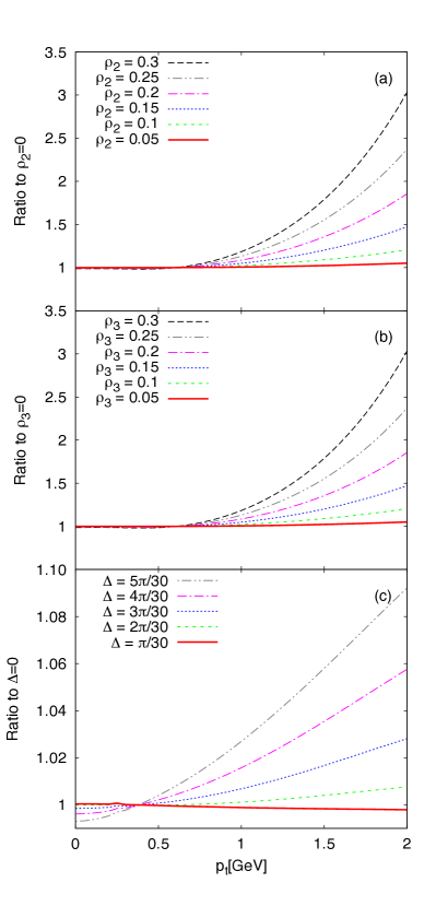
Before moving on towards the anisotropy it is interesting to explore if and how introducing spatial and flow anisotropy into the model modifies the azimuthally integrated single-particle spectrum. We have checked that if we introduce only a spatial anisotropy (i.e. the ansubscript𝑎𝑛a_{n} coefficients may be non-vanishing, but all ρnsubscript𝜌𝑛\rho_{n}’s are set to 0), then the normalisation may be slightly modified but the slope is unchanged. This is not the case for the flow anisotropy, however. As shown in Fig. 1a and Fig. 1b, flow anisotropy leads to slightly flatter spectra.
Refer to caption
Figure 1: The ratios of azimuthally integrated single particle spectra from fireballs with anisotropies to a reference spectrum calculated for the same set parameters except all anisotropy coefficients set to 0. Calculated for (directly produced) pions and T=120𝑇120T=120 MeV, ρ0=0.8subscript𝜌00.8\rho_{0}=0.8, R0=7subscript𝑅07R_{0}=7 fm, τ0=10subscript𝜏010\tau_{0}=10 fm/c𝑐c. (a) Ratios of spectra with second-order flow anisotropy and a2=a3=ρ3=0subscript𝑎2subscript𝑎3subscript𝜌30a_{2}=a_{3}=\rho_{3}=0. (b) Ratios of spectra with third-order flow anisotropy and a2=a3=ρ2=0subscript𝑎2subscript𝑎3subscript𝜌20a_{2}=a_{3}=\rho_{2}=0. (c) Ratios of spectra with a2=a3=ρ2=ρ3=0.1subscript𝑎2subscript𝑎3subscript𝜌2subscript𝜌30.1a_{2}=a_{3}=\rho_{2}=\rho_{3}=0.1 and different values of Δ=θ3θ2Δsubscript𝜃3subscript𝜃2\Delta=\theta_{3}-\theta_{2}.

We also show in Fig. 1c how the azimuthally integrated spectrum depends on the phase difference of the second and third order event planes (cf. Eq. (4))

Δ=θ3θ2.Δsubscript𝜃3subscript𝜃2\Delta=\theta_{3}-\theta_{2}\,. (14)

We do not expect any correlation between the second-order and the third-order event planes and to our knowledge there is no such correlation seen in the data. Hence, all phase differences are realised equally likely. In a data sample averaged over a large number of events the mean value of all observed curves would be measured.

Now we move on to the anisotropies of spectra which will be obtained as

vn=N1(pt,ϕ,Y)cos(n(ϕθn))𝑑ϕN1(pt,ϕ,Y)𝑑ϕ.subscript𝑣𝑛subscript𝑁1subscript𝑝𝑡italic-ϕ𝑌𝑛italic-ϕsubscript𝜃𝑛differential-ditalic-ϕsubscript𝑁1subscript𝑝𝑡italic-ϕ𝑌differential-ditalic-ϕv_{n}=\frac{\int N_{1}(p_{t},\phi,Y)\,\cos(n(\phi-\theta_{n}))\,d\phi}{\int N_{1}(p_{t},\phi,Y)\,d\phi}\,. (15)

The single-particle distributions are calculated via Eq. (12). The anisotropy coefficients vnsubscript𝑣𝑛v_{n} can be then expressed as

vn(pt)=Cn(pt)C0(pt)subscript𝑣𝑛subscript𝑝𝑡subscript𝐶𝑛subscript𝑝𝑡subscript𝐶0subscript𝑝𝑡v_{n}(p_{t})=\frac{C_{n}(p_{t})}{C_{0}(p_{t})} (16)

where

Cn(pt)=01𝑑r¯02π𝑑θr¯R2(θ)cos(n(θb(θ)θn))×In(ptsinhρ(r¯,θ)T)K1(ptcoshρ(r¯,θ)T)subscript𝐶𝑛subscript𝑝𝑡superscriptsubscript01differential-d¯𝑟superscriptsubscript02𝜋differential-d𝜃¯𝑟superscript𝑅2𝜃𝑛subscript𝜃𝑏𝜃subscript𝜃𝑛subscript𝐼𝑛subscript𝑝𝑡𝜌¯𝑟𝜃𝑇subscript𝐾1subscript𝑝𝑡𝜌¯𝑟𝜃𝑇C_{n}(p_{t})=\int_{0}^{1}d{\bar{r}}\int_{0}^{2\pi}d\theta\,{\bar{r}}\,R^{2}(\theta)\cos(n(\theta_{b}(\theta)-\theta_{n}))\\ \times I_{n}\left(\frac{p_{t}\sinh\rho({\bar{r}},\theta)}{T}\right)K_{1}\left(\frac{p_{t}\cosh\rho({\bar{r}},\theta)}{T}\right) (17)

where Insubscript𝐼𝑛I_{n} and K1subscript𝐾1K_{1} are modified Bessel functions and the integration over the azimuthal angle of the momentum ϕitalic-ϕ\phi was already performed here.

The result of the calculation, however, would depend on the value of the phase difference ΔΔ\Delta. This dependence is hidden in R(θ)𝑅𝜃R(\theta) and ρ(r¯,θ)𝜌¯𝑟𝜃\rho({\bar{r}},\theta). In an experimental analysis, one effectively takes an average over all its possible values. It has been shown in Lokos:2016fze that the averaging may have an effect on the results. We thus have to add this averaging and introduce

C¯n(pt)=023π𝑑Δ01𝑑r¯02π𝑑θr¯R2(θ)×cos(n(θb(θ)θn))×In(ptsinhρ(r¯,θ)T)K1(ptcoshρ(r¯,θ)T).subscript¯𝐶𝑛subscript𝑝𝑡superscriptsubscript023𝜋differential-dΔsuperscriptsubscript01differential-d¯𝑟superscriptsubscript02𝜋differential-d𝜃¯𝑟superscript𝑅2𝜃𝑛subscript𝜃𝑏𝜃subscript𝜃𝑛subscript𝐼𝑛subscript𝑝𝑡𝜌¯𝑟𝜃𝑇subscript𝐾1subscript𝑝𝑡𝜌¯𝑟𝜃𝑇\bar{C}_{n}(p_{t})=\int_{0}^{\frac{2}{3}\pi}d\Delta\int_{0}^{1}d{\bar{r}}\int_{0}^{2\pi}d\theta\,{\bar{r}}\,R^{2}(\theta)\\ \times\cos(n(\theta_{b}(\theta)-\theta_{n}))\\ \times I_{n}\left(\frac{p_{t}\sinh\rho({\bar{r}},\theta)}{T}\right)K_{1}\left(\frac{p_{t}\cosh\rho({\bar{r}},\theta)}{T}\right)\,. (18)

Then, the event-averaged vnsubscript𝑣𝑛v_{n} is obtained as

vn(pt)=C¯n(pt)C¯0(pt).subscript𝑣𝑛subscript𝑝𝑡subscript¯𝐶𝑛subscript𝑝𝑡subscript¯𝐶0subscript𝑝𝑡v_{n}(p_{t})=\frac{\bar{C}_{n}(p_{t})}{\bar{C}_{0}(p_{t})}\,. (19)

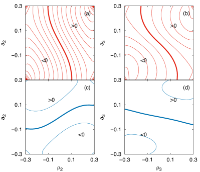
We calculated the dependence of v2subscript𝑣2v_{2} and v3subscript𝑣3v_{3} on the anisotropy coefficients ansubscript𝑎𝑛a_{n} and ρnsubscript𝜌𝑛\rho_{n}. We have checked that the vnsubscript𝑣𝑛v_{n}’s of given order basically depend only on coefficients of the same order, therefore we shall only investigate such same-order dependences. In Fig. 2 we show the contour plots where dependence on both spatial and flow anisotropy can be seen.
Refer to caption
Figure 2: Dependence of vnsubscript𝑣𝑛v_{n}’s on spatial anisotropy ansubscript𝑎𝑛a_{n} and flow anisotropy ρnsubscript𝜌𝑛\rho_{n} of the same order. Results are shown for pions (upper row) and protons (lower row) at pt=300subscript𝑝𝑡300p_{t}=300 MeV. Model parameters are T=120𝑇120T=120 MeV, ρ0=0.8subscript𝜌00.8\rho_{0}=0.8, R0=7subscript𝑅07R_{0}=7 fm, τ0=10subscript𝜏010\tau_{0}=10 fm/c𝑐c. The thick line identify v2subscript𝑣2v_{2} or v3subscript𝑣3v_{3} equal to 0, the thin lines correspond to increment or decrease of v2subscript𝑣2v_{2} (v3subscript𝑣3v_{3}) by 0.005.

A complex structure is observed. In general, we can conclude, similarly to Tomasik:2004bn ; Csanad:2008af ; Lokos:2016fze , that alone by measuring the anisotropy of single-particle distribution one is unable to determine uniquely both spatial and flow anisotropy. For heavy particles, like protons, vnsubscript𝑣𝑛v_{n}’s seem to be driven by the spatial anisotropy. Nevertheless, flow anisotropy kicks in as the value of ansubscript𝑎𝑛a_{n} grows. There is even a maximum assumed by v2subscript𝑣2v_{2} and v3subscript𝑣3v_{3} as a function of the corresponding ansubscript𝑎𝑛a_{n}, although it may well be beyond the phenomenologically relevant parameter region. The reason is that for high enough values of ansubscript𝑎𝑛a_{n} the outer surface of the fireball becomes concave and a smaller region moves transversely in the direction of the event plane. Although a unique combination of source parameters might possibly be determined from the combination of measurements with different particle species, a clear answer shall be provided by measuring the azimuthal dependence of the correlation radii.

4 Spatial anisotropy seen by femtoscopy

The femtoscopic technique which uses two-particle correlations is standard tool for measuring the space-time characteristics of the emitting source. Here we employ the standard formalism where the correlation function is defined as

C(p1,p2)=N2(p1,p2)N1(p1)N1(p2)=d6Ndp13dp23d3Ndp13d3Ndp23.𝐶subscript𝑝1subscript𝑝2subscript𝑁2subscript𝑝1subscript𝑝2subscript𝑁1subscript𝑝1subscript𝑁1subscript𝑝2superscript𝑑6𝑁𝑑superscriptsubscript𝑝13𝑑superscriptsubscript𝑝23superscript𝑑3𝑁𝑑superscriptsubscript𝑝13superscript𝑑3𝑁𝑑superscriptsubscript𝑝23C(p_{1},p_{2})=\frac{N_{2}(p_{1},p_{2})}{N_{1}(p_{1})N_{1}(p_{2})}=\frac{\frac{d^{6}N}{dp_{1}^{3}dp_{2}^{3}}}{\frac{d^{3}N}{dp_{1}^{3}}\frac{d^{3}N}{dp_{2}^{3}}}\,. (20)

Instead of the momenta of the two particles, the correlation function is usually parametrised in terms of the average momentum K𝐾K and the momentum difference q𝑞q

K𝐾\displaystyle K =\displaystyle= 12(p1+p2)12subscript𝑝1subscript𝑝2\displaystyle\frac{1}{2}(p_{1}+p_{2}) (21a)
q𝑞\displaystyle q =\displaystyle= p1p2.subscript𝑝1subscript𝑝2\displaystyle p_{1}-p_{2}\,. (21b)

Due to the on-shell constraint Kq=0𝐾𝑞0K\cdot q=0, the time component q0superscript𝑞0q^{0} can be expressed as

q0=KK0q=βq.superscript𝑞0𝐾superscript𝐾0𝑞𝛽𝑞q^{0}=\frac{\vec{K}}{K^{0}}\vec{q}=\vec{\beta}\vec{q}\,. (22)

Hence, only three spatial components of q𝑞q shall be taken as independent. Note that we have introduced the pair velocity β𝛽\vec{\beta}. The analysis is performed in the standard out-side-longitudinal reference frame where the outward direction is identified with the direction of the transverse component of K𝐾\vec{K} and the longitudinal axis is parallel to the beam. Correlation function is then measured for K𝐾\vec{K} from some interval and its inverse widths in q𝑞q carry information about space-time structure of the source. At given K𝐾\vec{K}-range one does not measure the size of the whole fireball but rather its homogeneity lengths. Those are the sizes of homogeneity regions. The homogeneity region is a part of the whole fireball which produces hadrons with momentum K𝐾K from a given range. Due to expansion it is usually smaller than the whole fireball. We shall particularly look at how the homogeneity lengths vary with the azimuthal angle ϕitalic-ϕ\phi of the K𝐾\vec{K} vector.

We will assume in what follows that the dependence of the correlation function on momentum difference q𝑞q can be reasonably well parametrised by a Gaussian prescription

C(q,K)1=exp(Ro2qo2Rs2qs2Rl2ql22Ros2qoqs2Rol2qoql2Rsl2qsql),𝐶𝑞𝐾1superscriptsubscript𝑅𝑜2superscriptsubscript𝑞𝑜2superscriptsubscript𝑅𝑠2superscriptsubscript𝑞𝑠2superscriptsubscript𝑅𝑙2superscriptsubscript𝑞𝑙22superscriptsubscript𝑅𝑜𝑠2subscript𝑞𝑜subscript𝑞𝑠2superscriptsubscript𝑅𝑜𝑙2subscript𝑞𝑜subscript𝑞𝑙2superscriptsubscript𝑅𝑠𝑙2subscript𝑞𝑠subscript𝑞𝑙C(q,K)-1=\exp\bigl{(}-R_{o}^{2}q_{o}^{2}-R_{s}^{2}q_{s}^{2}-R_{l}^{2}q_{l}^{2}\\ -2R_{os}^{2}q_{o}q_{s}-2R_{ol}^{2}q_{o}q_{l}-2R_{sl}^{2}q_{s}q_{l}\bigr{)}\,, (23)

where Rosubscript𝑅𝑜R_{o}, Rssubscript𝑅𝑠R_{s}, Rlsubscript𝑅𝑙R_{l}, Rossubscript𝑅𝑜𝑠R_{os}, Rolsubscript𝑅𝑜𝑙R_{ol}, and Rslsubscript𝑅𝑠𝑙R_{sl} are the correlation radii which can depend on K𝐾K. They will be directly calculated from the emission function, see below.

It is important to realise that the coordinate frame in which correlations are measured is specified by the hadrons used in the measurement. It is different from any coordinate system which is attached to the fireball. The rotation between the two frames defines the explicit angular dependence of the correlation radii. In addition to this, due to collective expansion of the fireball, hadrons flying in different directions come from different parts of the fireball and carry information about their homogeneity lengths. This introduces the implicit angular dependence of the correlation radii Heinz:2002au .

Generally, in the out-side-longitudinal system it can be derived that the correlation radii are given by the space-time variances as

Ro2(K)superscriptsubscript𝑅𝑜2𝐾\displaystyle R_{o}^{2}(K) =\displaystyle= (x~oβot~)2delimited-⟨⟩superscriptsubscript~𝑥𝑜subscript𝛽𝑜~𝑡2\displaystyle\left\langle(\tilde{x}_{o}-\beta_{o}\tilde{t})^{2}\right\rangle (24a)
Rs2(K)superscriptsubscript𝑅𝑠2𝐾\displaystyle R_{s}^{2}(K) =\displaystyle= xs2delimited-⟨⟩superscriptsubscript𝑥𝑠2\displaystyle\left\langle x_{s}^{2}\right\rangle (24b)
Rl2(K)superscriptsubscript𝑅𝑙2𝐾\displaystyle R_{l}^{2}(K) =\displaystyle= (x~lβlt~)2delimited-⟨⟩superscriptsubscript~𝑥𝑙subscript𝛽𝑙~𝑡2\displaystyle\left\langle(\tilde{x}_{l}-\beta_{l}\tilde{t})^{2}\right\rangle (24c)
Ros2(K)superscriptsubscript𝑅𝑜𝑠2𝐾\displaystyle R_{os}^{2}(K) =\displaystyle= (x~oβot~)x~sdelimited-⟨⟩subscript~𝑥𝑜subscript𝛽𝑜~𝑡subscript~𝑥𝑠\displaystyle\left\langle(\tilde{x}_{o}-\beta_{o}\tilde{t})\tilde{x}_{s}\right\rangle (24d)
Rol2(K)superscriptsubscript𝑅𝑜𝑙2𝐾\displaystyle R_{ol}^{2}(K) =\displaystyle= (x~oβot~)(x~lβlt~)delimited-⟨⟩subscript~𝑥𝑜subscript𝛽𝑜~𝑡subscript~𝑥𝑙subscript𝛽𝑙~𝑡\displaystyle\left\langle(\tilde{x}_{o}-\beta_{o}\tilde{t})(\tilde{x}_{l}-\beta_{l}\tilde{t})\right\rangle (24e)
Rsl2(K)superscriptsubscript𝑅𝑠𝑙2𝐾\displaystyle R_{sl}^{2}(K) =\displaystyle= x~s(x~lβlt~).delimited-⟨⟩subscript~𝑥𝑠subscript~𝑥𝑙subscript𝛽𝑙~𝑡\displaystyle\left\langle\tilde{x}_{s}(\tilde{x}_{l}-\beta_{l}\tilde{t})\right\rangle\,. (24f)

Note that the space-time variances depend on average momentum K𝐾K. Here we have introduced the averaging over the source

f(x)=S(x,p)f(x)d4xS(x,p)d4xdelimited-⟨⟩𝑓𝑥𝑆𝑥𝑝𝑓𝑥superscript𝑑4𝑥𝑆𝑥𝑝superscript𝑑4𝑥\langle f(x)\rangle=\frac{\int S(x,p)\,f(x)\,d^{4}x}{\int S(x,p)\,d^{4}x} (25)

and we also introduced the shifted coordinates as

x~μ=xμxμ.superscript~𝑥𝜇superscript𝑥𝜇delimited-⟨⟩superscript𝑥𝜇\tilde{x}^{\mu}=x^{\mu}-\langle x^{\mu}\rangle\,. (26)

Recall that the coordinates xosubscript𝑥𝑜x_{o}, xssubscript𝑥𝑠x_{s}, xlsubscript𝑥𝑙x_{l} are connected with the direction of the emitted particles. The explicit angular dependence is obtained simply by expressing the out-side-longitudinal coordinates in terms of the coordinates x𝑥x, y𝑦y, which are fixed with the fireball:

x~osubscript~𝑥𝑜\displaystyle\tilde{x}_{o} =\displaystyle= x~cosϕ+y~sinϕ~𝑥italic-ϕ~𝑦italic-ϕ\displaystyle\tilde{x}\cos\phi+\tilde{y}\sin\phi (27a)
x~ssubscript~𝑥𝑠\displaystyle\tilde{x}_{s} =\displaystyle= x~sinϕ+y~cosϕ.~𝑥italic-ϕ~𝑦italic-ϕ\displaystyle-\tilde{x}\sin\phi+\tilde{y}\cos\phi\,. (27b)

where ϕitalic-ϕ\phi is the azimuthal angle of the emitted hadron pairs. This leads to

Rs2superscriptsubscript𝑅𝑠2\displaystyle R_{s}^{2} =\displaystyle= 12(x~2+y~2)+12(x~2y~2)cos2ϕ12delimited-⟨⟩superscript~𝑥2delimited-⟨⟩superscript~𝑦212delimited-⟨⟩superscript~𝑥2delimited-⟨⟩superscript~𝑦22italic-ϕ\displaystyle\frac{1}{2}\left(\langle\tilde{x}^{2}\rangle+\langle\tilde{y}^{2}\rangle\right)+\frac{1}{2}\left(\langle\tilde{x}^{2}\rangle-\langle\tilde{y}^{2}\rangle\right)\cos 2\phi (28a)
x~y~sin2ϕdelimited-⟨⟩~𝑥~𝑦2italic-ϕ\displaystyle-\langle\tilde{x}\tilde{y}\rangle\sin 2\phi
Ro2superscriptsubscript𝑅𝑜2\displaystyle R_{o}^{2} =\displaystyle= 12(x~2+y~2)12(y~2x~2)cos2ϕ12delimited-⟨⟩superscript~𝑥2delimited-⟨⟩superscript~𝑦212delimited-⟨⟩superscript~𝑦2delimited-⟨⟩superscript~𝑥22italic-ϕ\displaystyle\frac{1}{2}\left(\left\langle\tilde{x}^{2}\right\rangle+\left\langle\tilde{y}^{2}\right\rangle\right)-\frac{1}{2}\left(\left\langle\tilde{y}^{2}\right\rangle-\left\langle\tilde{x}^{2}\right\rangle\right)\cos 2\phi (28b)
+x~y~sin2ϕ+βo2t~22βox~t~cosϕdelimited-⟨⟩~𝑥~𝑦2italic-ϕsuperscriptsubscript𝛽𝑜2delimited-⟨⟩superscript~𝑡22subscript𝛽𝑜delimited-⟨⟩~𝑥~𝑡italic-ϕ\displaystyle+\left\langle\tilde{x}\tilde{y}\right\rangle\sin 2\phi+\beta_{o}^{2}\left\langle\tilde{t}^{2}\right\rangle-2\beta_{o}\left\langle\tilde{x}\tilde{t}\right\rangle\cos\phi
2βoy~t~sinϕ2subscript𝛽𝑜delimited-⟨⟩~𝑦~𝑡italic-ϕ\displaystyle-2\beta_{o}\left\langle\tilde{y}\tilde{t}\right\rangle\sin\phi
Rl2superscriptsubscript𝑅𝑙2\displaystyle R_{l}^{2} =\displaystyle= (z~βlt~)2delimited-⟨⟩superscript~𝑧subscript𝛽𝑙~𝑡2\displaystyle\left\langle\left(\tilde{z}-\beta_{l}\tilde{t}\right)^{2}\right\rangle (28c)
Ros2superscriptsubscript𝑅𝑜𝑠2\displaystyle R_{os}^{2} =\displaystyle= x~y~cos2ϕ+12(y~2x~2)sin2ϕdelimited-⟨⟩~𝑥~𝑦2italic-ϕ12delimited-⟨⟩superscript~𝑦2delimited-⟨⟩superscript~𝑥22italic-ϕ\displaystyle\left\langle\tilde{x}\tilde{y}\right\rangle\cos 2\phi+\frac{1}{2}\left(\left\langle\tilde{y}^{2}\right\rangle-\left\langle\tilde{x}^{2}\right\rangle\right)\sin 2\phi (28d)
+βox~t~sinϕβoy~t~cosϕsubscript𝛽𝑜delimited-⟨⟩~𝑥~𝑡italic-ϕsubscript𝛽𝑜delimited-⟨⟩~𝑦~𝑡italic-ϕ\displaystyle+\beta_{o}\left\langle\tilde{x}\tilde{t}\right\rangle\sin\phi-\beta_{o}\left\langle\tilde{y}\tilde{t}\right\rangle\cos\phi
Rol2superscriptsubscript𝑅𝑜𝑙2\displaystyle R_{ol}^{2} =\displaystyle= (z~βlt~)x~cosϕ+(z~βlt~)y~sinϕdelimited-⟨⟩~𝑧subscript𝛽𝑙~𝑡~𝑥italic-ϕdelimited-⟨⟩~𝑧subscript𝛽𝑙~𝑡~𝑦italic-ϕ\displaystyle\left\langle\left(\tilde{z}-\beta_{l}\tilde{t}\right)\tilde{x}\right\rangle\cos\phi+\left\langle\left(\tilde{z}-\beta_{l}\tilde{t}\right)\tilde{y}\right\rangle\sin\phi (28e)
βl(z~βlt~)t~subscript𝛽𝑙delimited-⟨⟩~𝑧subscript𝛽𝑙~𝑡~𝑡\displaystyle-\beta_{l}\left\langle\left(\tilde{z}-\beta_{l}\tilde{t}\right)\tilde{t}\right\rangle
Rsl2superscriptsubscript𝑅𝑠𝑙2\displaystyle R_{sl}^{2} =\displaystyle= (z~βlt~)y~cosϕ(z~βlt~)x~sinϕ.delimited-⟨⟩~𝑧subscript𝛽𝑙~𝑡~𝑦italic-ϕdelimited-⟨⟩~𝑧subscript𝛽𝑙~𝑡~𝑥italic-ϕ\displaystyle\left\langle\left(\tilde{z}-\beta_{l}\tilde{t}\right)\tilde{y}\right\rangle\cos\phi-\left\langle\left(\tilde{z}-\beta_{l}\tilde{t}\right)\tilde{x}\right\rangle\sin\phi\,. (28f)

In what follows we want to study the azimuthal dependence of the correlation radii. To this end, they are customarily expanded into Fourier series. The space-time co-variances also depend non-trivially on ϕitalic-ϕ\phi, although we have suppressed writing this out explicitly. They can be written out and inserted in the right-hand sides of Eqs. (28). Then, by combining all sine and cosine terms on the r.h.s. of the obtained equations one can analytically identify all terms of Fourier expansion of the correlation radii. This has been done earlier for the second order Heinz:2002au ; Tomasik:2002rx . The results of the third and higher orders are presented in Appendix C.

In practical calculation, however, one can proceed differently. The whole azimuthal dependence can be calculated from Eqs. (28a)-(28f). Then one can extract any Fourier coefficient from the result. With increasing complexity of higher order terms this procedure appears computationally more efficient.

Moreover, these are not yet the correlation radii which correspond to the measured ones, even if the assumption of Gaussian correlation function is valid. In order to measure the correlation radii in real collisions, hadron pairs must be collected over a large number of events. The events must be rotated so that the event planes are all aligned. Otherwise the azimuthal dependence would be averaged out. For measuring the second-order oscillations one rotates the events so as to align the second-order event planes. For the third-order oscillation one aligns the third-order event planes. Since the event planes of different orders may be assumed to be uncorrelated these alignments effectively introduce averaging over the direction of the other event planes. This must be included in calculations. It has been investigated in Lokos:2016fze that this averaging may introduce a few percent effect on the resulting correlation radii. Hence, when calculating the correlation radii from Eqs. (28), one additional integral over θ2subscript𝜃2\theta_{2} or θ3subscript𝜃3\theta_{3} must be calculated, depending on which order of oscillations we shall be interested in. We include this averaging over other event planes in our calculation.

Therefore, the second order and the third order Fourier amplitudes that we are going to calculate do not belong to the same Fourier series. In the former case the emission function is averaged over all possible values of θ3subscript𝜃3\theta_{3}, in the latter averaging runs over θ2subscript𝜃2\theta_{2}. This will be also reflected in notation: the correlation radii will be expanded into series

Ri2(ϕ)=Ri,j,02+n=1Ri,j,n2cos(n(ϕϕn))superscriptsubscript𝑅𝑖2italic-ϕsuperscriptsubscript𝑅𝑖𝑗02superscriptsubscript𝑛1superscriptsubscript𝑅𝑖𝑗𝑛2𝑛italic-ϕsubscriptitalic-ϕ𝑛R_{i}^{2}(\phi)=R_{i,j,0}^{2}+\sum_{n=1}^{\infty}R_{i,j,n}^{2}\cos(n(\phi-\phi_{n})) (29)

where i=o,s𝑖𝑜𝑠i=o,s, and j=2,3𝑗23j=2,3, depending on which event plane θjsubscript𝜃𝑗\theta_{j} has been put to 0. In general, terms of the same order may differ, if they come from averaging with different event-planes fixed. For example, we note that

Ro,2,02superscriptsubscript𝑅𝑜202\displaystyle R_{o,2,0}^{2} \displaystyle\neq Ro,3,02superscriptsubscript𝑅𝑜302\displaystyle R_{o,3,0}^{2} (30a)
Rs,2,02superscriptsubscript𝑅𝑠202\displaystyle R_{s,2,0}^{2} \displaystyle\neq Rs,3,02.superscriptsubscript𝑅𝑠302\displaystyle R_{s,3,0}^{2}\,. (30b)

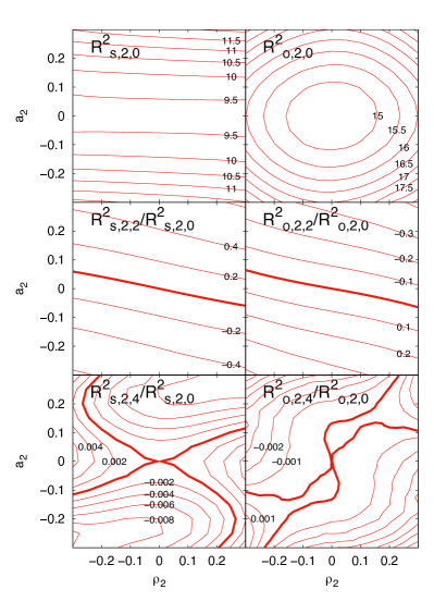
Second order oscillations have been calculated in Tomasik:2004bn , but the averaging over third order event plane was not performed there. In order to fill this gap, we have done the calculation here and show the results in Fig. 3
Refer to caption
Figure 3: The dependence of transverse correlation radii and their oscillation amplitudes on second-order anisotropies in space and transverse flow. The values are calculated for outward pair momentum Ko=300subscript𝐾𝑜300K_{o}=300 MeV. Model parameters used in the calculation are T=120𝑇120T=120 MeV, ρ0=0.8subscript𝜌00.8\rho_{0}=0.8, R0=7subscript𝑅07R_{0}=7 fm, τ0=10subscript𝜏010\tau_{0}=10 fm/c𝑐c. Third-order anisotropy parameters were set to a3=ρ3=0.1subscript𝑎3subscript𝜌30.1a_{3}=\rho_{3}=0.1.

The most important parameter which sets the scale of the transverse correlation radii is R0subscript𝑅0R_{0}. We can see that even the average radii Ri,2,02superscriptsubscript𝑅𝑖202R_{i,2,0}^{2} depend on both anisotropy parameters a2subscript𝑎2a_{2} and ρ2subscript𝜌2\rho_{2}. For the higher-order Fourier terms, we would like to factorise out their trivial scaling with R0subscript𝑅0R_{0}, thus for the analysis we divide all amplitudes by the zeroth-order term. As it was observed previously Tomasik:2004bn , the second order oscillation amplitude is mainly set by the spatial anisotropy parameter a2subscript𝑎2a_{2}. The dependence on ρ2subscript𝜌2\rho_{2} is weak. This confirms the early conjecture that the second-order spatial deformation can be measured with the help of correlation radii Tomasik:2004bn . Both spatial and flow anisotropy can then be obtained from combined measurement of v2subscript𝑣2v_{2} and the azimuthal dependence of correlation radii. Figure 3 also shows that in this model higher-order terms in the decomposition of the correlation radii are very small. The fourth-order terms are smaller than the second-order terms by two orders of magnitude. Although it shows an interesting dependence on a2subscript𝑎2a_{2} and ρ2subscript𝜌2\rho_{2}, it is most likely below any reasonable experimental sensitivity.

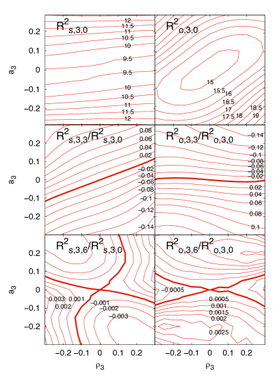
We have also looked at third-order oscillation in case of averaging over all possible directions of the second-order event plane. The resulting dependence of the correlation radii on a3subscript𝑎3a_{3} and ρ3subscript𝜌3\rho_{3} is plotted in Fig. 4.

Refer to caption
Figure 4: The dependence of transverse correlation radii and their oscillation amplitudes on third-order anisotropies in space and transverse flow. The values are calculated for outward pair momentum Ko=300subscript𝐾𝑜300K_{o}=300 MeV. Model parameters used in the calculation are T=120𝑇120T=120 MeV, ρ0=0.8subscript𝜌00.8\rho_{0}=0.8, R0=7subscript𝑅07R_{0}=7 fm, τ0=10subscript𝜏010\tau_{0}=10 fm/c𝑐c. Second-order anisotropy parameters were set to a2=ρ2=0.1subscript𝑎2subscript𝜌20.1a_{2}=\rho_{2}=0.1.

Again, even the azimuthally averaged radii show some dependence on both anisotropy parameters. The third-order spatial anisotropy is best reflected in the third-order scaled amplitude of the outward radii Ro,3,32/Ro,3,02superscriptsubscript𝑅𝑜332superscriptsubscript𝑅𝑜302R_{o,3,3}^{2}/R_{o,3,0}^{2}. For the sideward radius the third-order oscillation depends on both a3subscript𝑎3a_{3} and ρ3subscript𝜌3\rho_{3}. Note, however, that the third-order oscillation is typically smaller by an order of magnitude if it is compared to the second-order oscillation in Fig. 3. Even more suppressed is the next higher order, which is the sixth in this case. In absolute numbers the scaled amplitudes are on the level of a few per mille or even less. We do not expect that such a weak signal could be reasonably measured in experiments.

5 Relation to data

The present model has been designed with the aim to better characterise measured data on spectra and anisotropies. However, such an analysis requires to take into account many more issues and is technically much more involved. In order to reach physically relevant results, resonances must be included in the analysis Melo:2015wpa . This highly increases the complexity of calculations. Then, all data, i.e. identified spectra, anisotropy coefficients, and correlations, should be fitted simultaneously. The new Bayesian technique Bernhard:2016tnd seems well suitable to this aim. Such a thorough analysis, however, goes far beyond our scope here. Nevertheless, we want to illustrate the qualitative features presented in previous sections with the help of comparison to data. We hasten to stress that this comparison should be understood merely on qualitative level.

The STAR Collaboration has measured data from Au+Au collisions at sNN=200subscript𝑠𝑁𝑁200\sqrt{s_{NN}}=200 GeV. They have analysed second-order oscillations of correlation radii as functions of azimuthal angle with the blast-wave model extended to that order in Adams:2004yc . In that analysis, the temperature T𝑇T and transverse flow gradient ρ0subscript𝜌0\rho_{0} were inferred from a simultaneous fit to pion, kaon, and proton ptsubscript𝑝𝑡p_{t} spectra and v2subscript𝑣2v_{2}. Analysis of the azimuthally sensitive correlation radii yielded the sizes of the fireball and the second-order anisotropy parameters. From this analysis of 10-20% centrality STAR data, the following model parameter values have been extracted by the STAR Collaboration Adams:2004yc : T=98𝑇98T=98 MeV, ρ0=0.98subscript𝜌00.98\rho_{0}=0.98, ρ2=0.05subscript𝜌20.05\rho_{2}=0.05, τ0=7.8subscript𝜏07.8\tau_{0}=7.8 fm/c𝑐c, Δτ=2.59Δ𝜏2.59\Delta\tau=2.59 fm/c𝑐c. The second-order spatial anisotropy can be translated into our model as R0=11.4subscript𝑅011.4R_{0}=11.4 fm, a2=0.0439subscript𝑎20.0439a_{2}=0.0439.

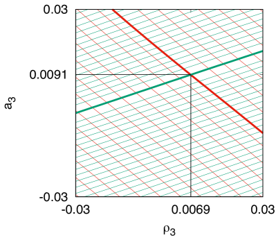
With these values fixed we calculate the combined contour plot for the dependences of v3subscript𝑣3v_{3} and third-order scaled amplitude Rs,3,32/Rs,3,02superscriptsubscript𝑅𝑠332superscriptsubscript𝑅𝑠302R_{s,3,3}^{2}/R_{s,3,0}^{2} on a3subscript𝑎3a_{3} and ρ3subscript𝜌3\rho_{3}. It is shown in Fig. 5.

Refer to caption
Figure 5: Combined contour lines of constant v3subscript𝑣3v_{3} (red from top left to bottom right) and constant Rs,3,32/Rs,0,32superscriptsubscript𝑅𝑠332superscriptsubscript𝑅𝑠032R_{s,3,3}^{2}/R_{s,0,3}^{2} (green from bottom left to top right). Thick lines show the values of data for pt=863subscript𝑝𝑡863p_{t}=863 MeV (v3subscript𝑣3v_{3}) Adare:2011tg and Kt=877subscript𝐾𝑡877K_{t}=877 MeV (correlation radii) Adare:2014vax . The increment between neighbouring lines is 0.01.

The curves decreasing to the right are lines with constant v3subscript𝑣3v_{3}, the others correspond to constant Rs,3,32/Rs,0,32superscriptsubscript𝑅𝑠332superscriptsubscript𝑅𝑠032R_{s,3,3}^{2}/R_{s,0,3}^{2}. Thick lines represent the data values by PHENIX Adare:2011tg ; Adare:2014vax . Out of available data we had to choose bins in ptsubscript𝑝𝑡p_{t} for v3subscript𝑣3v_{3} and correlation radii, which overlap. Unfortunately, these two sets of data are measured in slightly different momentum ranges. In order to use overlapping ptsubscript𝑝𝑡p_{t} bins, we have taken v3subscript𝑣3v_{3} point for pions at pt=863subscript𝑝𝑡863p_{t}=863 MeV Adare:2011tg and correlation radii for Kt=877subscript𝐾𝑡877K_{t}=877 MeV Adare:2014vax . The values extracted from such a simple comparison with data are: a3=0.0091subscript𝑎30.0091a_{3}=0.0091 and ρ3=0.0069subscript𝜌30.0069\rho_{3}=0.0069.

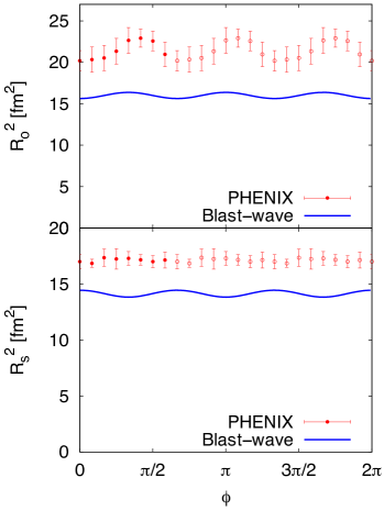
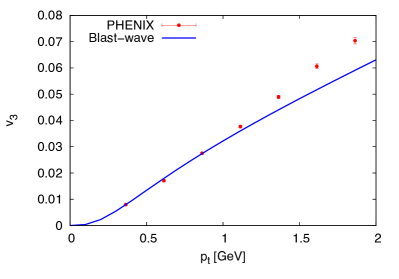
With the extracted model parameters we tried to calculate theoretical predictions for v3subscript𝑣3v_{3} (Fig. 6) and the azimuthal angle dependence of the correlation radii (Fig. 7).
Refer to caption
Figure 6: The ptsubscript𝑝𝑡p_{t} dependence of v3subscript𝑣3v_{3} for identified pions measured by PHENIX collaboration Adare:2011tg compared with the theoretical curve from the blast-wave model with parameters determined in Fig. 5.
Refer to caption
Figure 7: The azimuthal dependence of correlation radii with respect to the third-order event plane for Kt=530subscript𝐾𝑡530K_{t}=530 MeV/c𝑐c. Data by PHENIX collaboration Adare:2014vax are compared with results from the blast-wave model with parameters determined in Fig. 5.

For the latter we chose to plot the radii measured for Kt=530subscript𝐾𝑡530K_{t}=530 MeV/c𝑐c as was also done by the PHENIX Collaboration in Adare:2014vax . The model fails completely in reproducing the absolute size of the correlation radii. The corresponding parameter, however, has been fixed from the STAR analysis of second-order oscillations of correlation radii. The mean values of the radii should be very similar for second and the third order oscillations. This clearly demonstrates the need of simultaneous fit to all available data in single analysis if one wants to go beyond the qualitative level.

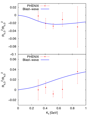
We also show in Fig. 8 the third-order scaled amplitudes of correlation radii as functions of Ktsubscript𝐾𝑡K_{t}.

Refer to caption
Figure 8: The Ktsubscript𝐾𝑡K_{t} dependence of third-order oscillation amplitude of the correlation radii. Data by PHENIX collaboration Adare:2014vax are compared with results from the blast-wave model with parameters determined in Fig. 5.

The experimental error bars are huge and we explained that we have based our analysis on the point at highest Ktsubscript𝐾𝑡K_{t}. It seems that the PHENIX data require amplitudes of opposite signs, which the blast-wave model can accommodate.

We want to close this section with a few comments on the applicability of the model to preliminary ALICE data from Pb+Pb collisions at sNN=2.76subscript𝑠𝑁𝑁2.76\sqrt{s_{NN}}=2.76 TeV ALICE@WPCF . The data seem to indicate that the third-order oscillation amplitudes of both Rs2superscriptsubscript𝑅𝑠2R_{s}^{2} and Ro2superscriptsubscript𝑅𝑜2R_{o}^{2} are negative. By inspecting Fig. 4 we find that such situation only happens in a small region in parameter space with a3subscript𝑎3a_{3} around 0 and positive ρ3subscript𝜌3\rho_{3}. Thus from combined measurements of outward and sideward radii one could deduce that the fireball at the LHC has rather symmetric shape and the anisotropy is set by the transverse collective velocity field.

6 Conclusions

We have generalised the blast-wave model so that it includes third-order anisotropies in both space and expansion. Analogically to the second order, from the combination of Fig. 2 and Fig. 4 we can infer, that it is indeed possible to reconstruct both anisotropy coefficients of this model: a3subscript𝑎3a_{3} and ρ3subscript𝜌3\rho_{3}, from measurements of the azimuthal anisotropy of single-particle momentum distributions and HBT radii.

We have also pointed out the need for averaging over the difference of second and third-order reaction planes when focusing on a selected order of Fourier decomposition of the hadron distribution or the correlation radii. This is effectively done in data analysis when all events are aligned according to the event plane of the selected order.

The contour plots shown in Fig. 4 exemplify the statement made in Plumberg:2013nga that at fixed flow anisotropy the amplitude of correlation radii oscillation can be tuned with the help of spatial anisotropy and even a flip in the phase can be obtained. Such a flip of the phase corresponds to a change of the sign of the amplitude. Keeping constant flow anisotropy and changing space anisotropy corresponds to moving vertically in the panels of Fig. 4 and the phase flip corresponds to crossing the thick line in that Figure. Our results are much more detailed since we show the full dependence on the two parameters.

We have also calculated the subleading terms for the third-order anisotropies in the oscillations of correlation radii. These are the sixth-order oscillations. They were shown to be an order of magnitude smaller than the lower order and hardly measurable at current experimental statistics. We have actually derived expressions for oscillation amplitudes at general order, but there is currently no need to go to higher orders also with model studies as sufficient statistics would hardly be available.
Refer to caption
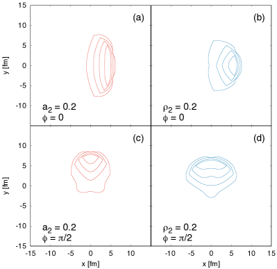
Figure 9: Transverse profiles of the emission function for the blast-wave model with source parameters as in Fig. 4, for particles with pt=300subscript𝑝𝑡300p_{t}=300 MeV in the indicated direction ϕitalic-ϕ\phi. Left column: only density profile anisotropy; right column: only flow anisotropy. Other source parameters are T=120𝑇120T=120 MeV, τ0=10subscript𝜏010\tau_{0}=10 fm, R0=7subscript𝑅07R_{0}=7 fm, Δτ=1Δ𝜏1\Delta\tau=1 fm, ρ0=0.8subscript𝜌00.8\rho_{0}=0.8. Shown are the effective sources which are calculated by integrating over all directions of the third-order anisotropy with a3=ρ3=0.1subscript𝑎3subscript𝜌30.1a_{3}=\rho_{3}=0.1. The contours correspond to levels of 0.8, 0.6, 0.4, and 0.2 of the maximum.
Refer to caption
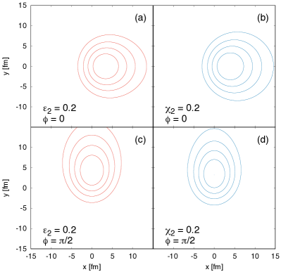
Figure 10: Analogical to Fig. 9, but calculated with the Buda-Lund model, with source parameters T=120𝑇120T=120 MeV, τ0=10subscript𝜏010\tau_{0}=10 fm, a2=0.3subscript𝑎20.3a_{2}=0.3, b=0.1𝑏0.1b=-0.1, R=7𝑅7R=7, Z=15𝑍15Z=15, H=8𝐻8H=8, Hz=16subscript𝐻𝑧16H_{z}=16, ϵ3=χ3=0.1subscriptitalic-ϵ3subscript𝜒30.1\epsilon_{3}=\chi_{3}=0.1. The model is explained in Lokos:2016fze . The values of the second-order anisotropy parameters are indicated in the figure. The averaging over all directions of the third-order anisotropy is performed with ε3=χ3=0.1subscript𝜀3subscript𝜒30.1\varepsilon_{3}=\chi_{3}=0.1.

It is interesting to compare our results to those obtained in an analogical study which used the Buda-Lund model Lokos:2016fze . In that model, the way in which observables depend on the combination of the space and flow anisotropy is different to the one presented here. Partially, this is due to our definition of the spatial profile with the minus sign in Eq. (4). The corresponding sign in the Buda-Lund model was kept to be plus. On the qualitative level, the oscillations of the correlation radii within the Buda-Lund model seem to be much more sensitive to the flow anisotropy than it is the case in this study.

In order to explore the difference of the two models in more details, in Figs. 9 and 10 we plot transverse profiles of the emitting sources according to the blast-wave and Buda-Lund models, respectively. Plotted are not the emission functions directly. We have assumed that there are the third-order anisotropies, as well, which have their third-order event planes completely independent from the second-order event plane directions. Then, we have integrated over all possible directions of the third-order event plane and obtained an effective emission function with only second-order anisotropy. In the figures, we have assumed pions with pt=300subscript𝑝𝑡300p_{t}=300 MeV and two different azimuthal angles of particle emission: ϕ=0italic-ϕ0\phi=0 (upper rows) and ϕ=π/2italic-ϕ𝜋2\phi=\pi/2 (lower rows).

Figures 9 and 10 clearly demonstrate that the two models behave rather differently. In the Buda-Lund model, the deformations caused by the density anisotropy (Fig. 10 left) and by flow anisotropy (Fig. 10 right) look qualitatively similar. On the other hand, the sharp source boundary in the blast wave model has severe influence. The spatial anisotropy (Fig. 9 left) makes the two sources for ϕ=0italic-ϕ0\phi=0 and ϕ=π/2italic-ϕ𝜋2\phi=\pi/2 qualitatively much more different from each other than the flow anisotropy (Fig. 9 right). Note that the sources should be compared in the out-side-long coordinate system, and the outward axis is directed in the direction of ϕitalic-ϕ\phi. Thus we see the much stronger dependence on shape anisotropy than on flow anisotropy.

Having the two models which appear so differently, the choice of the more suitable model should be decided by data. Note, however, that neither this schematic study, nor the one of ref. Lokos:2016fze included meson production from the decays of resonances and the modification of the correlation function due to viscosity. Their influence should be investigated in the future in order to arrive at a conclusive answer.

Acknowledgements.
This work has been performed in framework of COST Action CA15213 “Theory of hot matter and relativistic heavy-ion collisions” (THOR). Partial support by VEGA 1/0469/15 (Slovakia) and by MŠMT grant No. LG15001 (Czech Republic) is acknowledged. M. Cs. was supported by the János Bolyai Research Scholarship of the Hungarian Academy of Sciences.

Appendix A Relation between different parametrisations of second-order spatial anisotropy

In this Appendix we derive the relation between our parametrisation of the transverse shape and the one used in Tomasik:2004bn .

First of all, it should be clearly stated that the two parametrisations are different. Hence, the elliptic shape that has been used in Tomasik:2004bn would be fully reproduced with the help of parametrisation (4) only if higher-order terms are included. Of course, the importance of higher orders drops with n𝑛n.

We shall assume here that the second-order anisotropy is small, i.e., the parameter a𝑎a from Eq. (5) is close to 1. The ellipse of Tomasik:2004bn includes points with coordinates

rxsubscript𝑟𝑥\displaystyle r_{x} =\displaystyle= Rxcosθ=aRcosθsubscript𝑅𝑥𝜃𝑎superscript𝑅𝜃\displaystyle R_{x}\cos\theta=aR^{\prime}\cos\theta (31a)
rysubscript𝑟𝑦\displaystyle r_{y} =\displaystyle= Rysinθ=Rasinθ.subscript𝑅𝑦𝜃superscript𝑅𝑎𝜃\displaystyle R_{y}\sin\theta=\frac{R^{\prime}}{a}\sin\theta\,. (31b)

Thus the radius as function of the azimuthal angle is

R=rx2+ry2=a2R2cos2θ+R2a2sin2θ.𝑅superscriptsubscript𝑟𝑥2superscriptsubscript𝑟𝑦2superscript𝑎2superscriptsuperscript𝑅2superscript2𝜃superscriptsuperscript𝑅2superscript𝑎2superscript2𝜃R=\sqrt{r_{x}^{2}+r_{y}^{2}}=\sqrt{a^{2}{R^{\prime}}^{2}\cos^{2}\theta+\frac{{R^{\prime}}^{2}}{a^{2}}\sin^{2}\theta}\,. (32)

This can be rewritten as

R=Ra4+12a2(1+a41a4+1cos(2θ))12.𝑅superscript𝑅superscript𝑎412superscript𝑎2superscript1superscript𝑎41superscript𝑎412𝜃12R=R^{\prime}\sqrt{\frac{a^{4}+1}{2a^{2}}}\left(1+\frac{a^{4}-1}{a^{4}+1}\cos(2\theta)\right)^{\frac{1}{2}}\,. (33)

Now we assume that a1𝑎1a\to 1 and therefore (a41)/(a4+1)superscript𝑎41superscript𝑎41(a^{4}-1)/(a^{4}+1) is very small. Thus we can Taylor-expand the bracket up to first order and obtain

R(θ)Ra4+12a2(1+12a41a4+1cos(2θ)).𝑅𝜃superscript𝑅superscript𝑎412superscript𝑎2112superscript𝑎41superscript𝑎412𝜃R(\theta)\approx R^{\prime}\sqrt{\frac{a^{4}+1}{2a^{2}}}\left(1+\frac{1}{2}\frac{a^{4}-1}{a^{4}+1}\cos(2\theta)\right)\,. (34)

The mean radius R0subscript𝑅0R_{0} of the present model is to be identified with

R0=Ra4+12a2.subscript𝑅0superscript𝑅superscript𝑎412superscript𝑎2R_{0}=R^{\prime}\sqrt{\frac{a^{4}+1}{2a^{2}}}\,. (35)

The amplitude of the oscillations is to be identified with (a2)subscript𝑎2(-a_{2})

a2=12a41a4+1.subscript𝑎212superscript𝑎41superscript𝑎41a_{2}=-\frac{1}{2}\frac{a^{4}-1}{a^{4}+1}\,. (36)

Inverting this relation gives

a=(12a21+2a2)14.𝑎superscript12subscript𝑎212subscript𝑎214a=\left(\frac{1-2a_{2}}{1+2a_{2}}\right)^{\frac{1}{4}}\,. (37)

Appendix B The direction of transverse velocity

Here we derive the direction of the transverse velocity, which is given by the angle θbsubscript𝜃𝑏\theta_{b}. Since it is supposed to be perpendicular to the surface of constant r¯¯𝑟{\bar{r}}, we write down its coordinates

x𝑥\displaystyle x =\displaystyle= r¯R0(1n=2ancos(n(θθn)))cosθ¯𝑟subscript𝑅01superscriptsubscript𝑛2subscript𝑎𝑛𝑛𝜃subscript𝜃𝑛𝜃\displaystyle{\bar{r}}R_{0}\left(1-\sum_{n=2}^{\infty}a_{n}\cos(n(\theta-\theta_{n}))\right)\cos\theta (38a)
y𝑦\displaystyle y =\displaystyle= r¯R0(1n=2ancos(n(θθn)))sinθ.¯𝑟subscript𝑅01superscriptsubscript𝑛2subscript𝑎𝑛𝑛𝜃subscript𝜃𝑛𝜃\displaystyle{\bar{r}}R_{0}\left(1-\sum_{n=2}^{\infty}a_{n}\cos(n(\theta-\theta_{n}))\right)\sin\theta\,. (38b)

In further calculations, however, we shall truncate the expansion after the third-order term.

The (truncated) expressions (38) can be inserted into the derivatives in Eq. (10). This gives

θb=π2+arctanAB.subscript𝜃𝑏𝜋2𝐴𝐵\theta_{b}=\frac{\pi}{2}+\arctan\frac{A}{B}\,. (39)

where

A=4a2sinθ+3a3sin3(θθ3)cosθ1+a2cos2(θθ2)+a3cos3(θθ3)sinθ𝐴4subscript𝑎2𝜃3subscript𝑎33𝜃subscript𝜃3𝜃1subscript𝑎22𝜃subscript𝜃2subscript𝑎33𝜃subscript𝜃3𝜃A=4a_{2}\sin\theta+3a_{3}\frac{\sin 3(\theta-\theta_{3})}{\cos\theta}\\ -\frac{-1+a_{2}\cos 2(\theta-\theta_{2})+a_{3}\cos 3(\theta-\theta_{3})}{\sin\theta} (40)
B=a2cosθ+3a3sin3(θθ3)sinθ1+a2cos2(θθ2)+a3cos3(θθ3)cosθ𝐵subscript𝑎2𝜃3subscript𝑎33𝜃subscript𝜃3𝜃1subscript𝑎22𝜃subscript𝜃2subscript𝑎33𝜃subscript𝜃3𝜃B=a_{2}\cos\theta+3a_{3}\frac{\sin 3(\theta-\theta_{3})}{\sin\theta}\\ -\frac{-1+a_{2}\cos 2(\theta-\theta_{2})+a_{3}\cos 3(\theta-\theta_{3})}{\cos\theta} (41)

Appendix C Fourier amplitudes of the correlation radii

Here we give an overview of the Fourier amplitudes of the azimuthal dependence of outward, sideward, and out-side cross-term correlation radii. Note that these formulas are model-independent. Dependence on a particular model comes into evaluation of individual space-time (co-)variances. Note that analogical relations have been derived in Plumberg:2013nga , where Milne coordinates were used instead of the Cartesian ones.

We define the amplitudes

Ro2superscriptsubscript𝑅𝑜2\displaystyle R_{o}^{2} =\displaystyle= (Ro2)0+n=1[(Ro2)nssin(nϕ)+(Ro2)nccos(nϕ)]subscriptsuperscriptsubscript𝑅𝑜20superscriptsubscript𝑛1delimited-[]superscriptsubscriptsuperscriptsubscript𝑅𝑜2𝑛𝑠𝑛italic-ϕsuperscriptsubscriptsuperscriptsubscript𝑅𝑜2𝑛𝑐𝑛italic-ϕ\displaystyle\left(R_{o}^{2}\right)_{0}+\sum_{n=1}^{\infty}\left[\left(R_{o}^{2}\right)_{n}^{s}\sin(n\phi)+\left(R_{o}^{2}\right)_{n}^{c}\cos(n\phi)\right]
Rs2superscriptsubscript𝑅𝑠2\displaystyle R_{s}^{2} =\displaystyle= (Rs2)0+n=1[(Rs2)nssin(nϕ)+(Rs2)nccos(nϕ)]subscriptsuperscriptsubscript𝑅𝑠20superscriptsubscript𝑛1delimited-[]superscriptsubscriptsuperscriptsubscript𝑅𝑠2𝑛𝑠𝑛italic-ϕsuperscriptsubscriptsuperscriptsubscript𝑅𝑠2𝑛𝑐𝑛italic-ϕ\displaystyle\left(R_{s}^{2}\right)_{0}+\sum_{n=1}^{\infty}\left[\left(R_{s}^{2}\right)_{n}^{s}\sin(n\phi)+\left(R_{s}^{2}\right)_{n}^{c}\cos(n\phi)\right]
Ros2superscriptsubscript𝑅𝑜𝑠2\displaystyle R_{os}^{2} =\displaystyle= (Ros2)0+n=1[(Ros2)nssin(nϕ)+(Ros2)nccos(nϕ)]subscriptsuperscriptsubscript𝑅𝑜𝑠20superscriptsubscript𝑛1delimited-[]superscriptsubscriptsuperscriptsubscript𝑅𝑜𝑠2𝑛𝑠𝑛italic-ϕsuperscriptsubscriptsuperscriptsubscript𝑅𝑜𝑠2𝑛𝑐𝑛italic-ϕ\displaystyle\left(R_{os}^{2}\right)_{0}+\sum_{n=1}^{\infty}\left[\left(R_{os}^{2}\right)_{n}^{s}\sin(n\phi)+\left(R_{os}^{2}\right)_{n}^{c}\cos(n\phi)\right]

In a similar way we shall expand the space-time (co-)variances

x~μx~ν=x~μx~ν0+n=1[x~μx~νnssin(nϕ)+x~μx~νnccos(nϕ)]delimited-⟨⟩superscript~𝑥𝜇superscript~𝑥𝜈subscriptdelimited-⟨⟩superscript~𝑥𝜇superscript~𝑥𝜈0superscriptsubscript𝑛1delimited-[]superscriptsubscriptdelimited-⟨⟩superscript~𝑥𝜇superscript~𝑥𝜈𝑛𝑠𝑛italic-ϕsuperscriptsubscriptdelimited-⟨⟩superscript~𝑥𝜇superscript~𝑥𝜈𝑛𝑐𝑛italic-ϕ\left\langle\tilde{x}^{\mu}\tilde{x}^{\nu}\right\rangle=\left\langle\tilde{x}^{\mu}\tilde{x}^{\nu}\right\rangle_{0}\\ +\sum_{n=1}^{\infty}\left[\left\langle\tilde{x}^{\mu}\tilde{x}^{\nu}\right\rangle_{n}^{s}\sin(n\phi)+\left\langle\tilde{x}^{\mu}\tilde{x}^{\nu}\right\rangle_{n}^{c}\cos(n\phi)\right] (43)

The series (43) are inserted into the model-independent expressions (28) and the sine and cosine terms are reorganised with the help of addition theorems. Then one can collect the terms order by order and put them in equality with the corresponding expansion of the correlation radii. We obtain for the outward radius

(Ro2)0subscriptsuperscriptsubscript𝑅𝑜20\displaystyle(R_{o}^{2})_{0} =\displaystyle= 12x~20+12y~2014y~22c+14x~22c12subscriptdelimited-⟨⟩superscript~𝑥2012subscriptdelimited-⟨⟩superscript~𝑦2014superscriptsubscriptdelimited-⟨⟩superscript~𝑦22𝑐14superscriptsubscriptdelimited-⟨⟩superscript~𝑥22𝑐\displaystyle\frac{1}{2}\left\langle\tilde{x}^{2}\right\rangle_{0}+\frac{1}{2}\left\langle\tilde{y}^{2}\right\rangle_{0}-\frac{1}{4}\left\langle\tilde{y}^{2}\right\rangle_{2}^{c}+\frac{1}{4}\left\langle\tilde{x}^{2}\right\rangle_{2}^{c} (44a)
+12x~y~2s+βo2t~20βot~x~1c12superscriptsubscriptdelimited-⟨⟩~𝑥~𝑦2𝑠superscriptsubscript𝛽𝑜2subscriptdelimited-⟨⟩superscript~𝑡20subscript𝛽𝑜superscriptsubscriptdelimited-⟨⟩~𝑡~𝑥1𝑐\displaystyle+\frac{1}{2}\left\langle\tilde{x}\tilde{y}\right\rangle_{2}^{s}+\beta_{o}^{2}\left\langle\tilde{t}^{2}\right\rangle_{0}-\beta_{o}\left\langle\tilde{t}\tilde{x}\right\rangle_{1}^{c}
βot~y~1ssubscript𝛽𝑜superscriptsubscriptdelimited-⟨⟩~𝑡~𝑦1𝑠\displaystyle-\beta_{o}\left\langle\tilde{t}\tilde{y}\right\rangle_{1}^{s}
(Ro2)1csuperscriptsubscriptsuperscriptsubscript𝑅𝑜21𝑐\displaystyle(R_{o}^{2})_{1}^{c} =\displaystyle= 34x~21c+14y~21c14y~23c+14x~23c34superscriptsubscriptdelimited-⟨⟩superscript~𝑥21𝑐14superscriptsubscriptdelimited-⟨⟩superscript~𝑦21𝑐14superscriptsubscriptdelimited-⟨⟩superscript~𝑦23𝑐14superscriptsubscriptdelimited-⟨⟩superscript~𝑥23𝑐\displaystyle\frac{3}{4}\left\langle\tilde{x}^{2}\right\rangle_{1}^{c}+\frac{1}{4}\left\langle\tilde{y}^{2}\right\rangle_{1}^{c}-\frac{1}{4}\left\langle\tilde{y}^{2}\right\rangle_{3}^{c}+\frac{1}{4}\left\langle\tilde{x}^{2}\right\rangle_{3}^{c} (44b)
+12(x~y~1s+x~y~3s)+βo2t~21c2βot~x~012superscriptsubscriptdelimited-⟨⟩~𝑥~𝑦1𝑠superscriptsubscriptdelimited-⟨⟩~𝑥~𝑦3𝑠superscriptsubscript𝛽𝑜2superscriptsubscriptdelimited-⟨⟩superscript~𝑡21𝑐2subscript𝛽𝑜subscriptdelimited-⟨⟩~𝑡~𝑥0\displaystyle+\frac{1}{2}\left(\left\langle\tilde{x}\tilde{y}\right\rangle_{1}^{s}+\left\langle\tilde{x}\tilde{y}\right\rangle_{3}^{s}\right)+\beta_{o}^{2}\left\langle\tilde{t}^{2}\right\rangle_{1}^{c}-2\beta_{o}\left\langle\tilde{t}\tilde{x}\right\rangle_{0}
βot~x~2cβot~y~2ssubscript𝛽𝑜superscriptsubscriptdelimited-⟨⟩~𝑡~𝑥2𝑐subscript𝛽𝑜superscriptsubscriptdelimited-⟨⟩~𝑡~𝑦2𝑠\displaystyle-\beta_{o}\left\langle\tilde{t}\tilde{x}\right\rangle_{2}^{c}-\beta_{o}\left\langle\tilde{t}\tilde{y}\right\rangle_{2}^{s}
(Ro2)1ssuperscriptsubscriptsuperscriptsubscript𝑅𝑜21𝑠\displaystyle(R_{o}^{2})_{1}^{s} =\displaystyle= 14x~21s+34y~21s+14y~23s14x~23s14superscriptsubscriptdelimited-⟨⟩superscript~𝑥21𝑠34superscriptsubscriptdelimited-⟨⟩superscript~𝑦21𝑠14superscriptsubscriptdelimited-⟨⟩superscript~𝑦23𝑠14superscriptsubscriptdelimited-⟨⟩superscript~𝑥23𝑠\displaystyle\frac{1}{4}\left\langle\tilde{x}^{2}\right\rangle_{1}^{s}+\frac{3}{4}\left\langle\tilde{y}^{2}\right\rangle_{1}^{s}+\frac{1}{4}\left\langle\tilde{y}^{2}\right\rangle_{3}^{s}-\frac{1}{4}\left\langle\tilde{x}^{2}\right\rangle_{3}^{s} (44c)
+12(x~y~1cx~y~3c)+βo2t~21sβot~x~2s12superscriptsubscriptdelimited-⟨⟩~𝑥~𝑦1𝑐superscriptsubscriptdelimited-⟨⟩~𝑥~𝑦3𝑐superscriptsubscript𝛽𝑜2superscriptsubscriptdelimited-⟨⟩superscript~𝑡21𝑠subscript𝛽𝑜superscriptsubscriptdelimited-⟨⟩~𝑡~𝑥2𝑠\displaystyle+\frac{1}{2}\left(\left\langle\tilde{x}\tilde{y}\right\rangle_{1}^{c}-\left\langle\tilde{x}\tilde{y}\right\rangle_{3}^{c}\right)+\beta_{o}^{2}\left\langle\tilde{t}^{2}\right\rangle_{1}^{s}-\beta_{o}\left\langle\tilde{t}\tilde{x}\right\rangle_{2}^{s}
2βot~y~0+βot~y~2c2subscript𝛽𝑜subscriptdelimited-⟨⟩~𝑡~𝑦0subscript𝛽𝑜superscriptsubscriptdelimited-⟨⟩~𝑡~𝑦2𝑐\displaystyle-2\beta_{o}\left\langle\tilde{t}\tilde{y}\right\rangle_{0}+\beta_{o}\left\langle\tilde{t}\tilde{y}\right\rangle_{2}^{c}
(Ro2)2csuperscriptsubscriptsuperscriptsubscript𝑅𝑜22𝑐\displaystyle(R_{o}^{2})_{2}^{c} =\displaystyle= 12x~22c+12y~22c12y~2014y~24c12superscriptsubscriptdelimited-⟨⟩superscript~𝑥22𝑐12superscriptsubscriptdelimited-⟨⟩superscript~𝑦22𝑐12subscriptdelimited-⟨⟩superscript~𝑦2014superscriptsubscriptdelimited-⟨⟩superscript~𝑦24𝑐\displaystyle\frac{1}{2}\left\langle\tilde{x}^{2}\right\rangle_{2}^{c}+\frac{1}{2}\left\langle\tilde{y}^{2}\right\rangle_{2}^{c}-\frac{1}{2}\left\langle\tilde{y}^{2}\right\rangle_{0}-\frac{1}{4}\left\langle\tilde{y}^{2}\right\rangle_{4}^{c} (44d)
+12x~20+14x~24c+12x~y~4s+βo2t~22c12subscriptdelimited-⟨⟩superscript~𝑥2014superscriptsubscriptdelimited-⟨⟩superscript~𝑥24𝑐12superscriptsubscriptdelimited-⟨⟩~𝑥~𝑦4𝑠superscriptsubscript𝛽𝑜2superscriptsubscriptdelimited-⟨⟩superscript~𝑡22𝑐\displaystyle+\frac{1}{2}\left\langle\tilde{x}^{2}\right\rangle_{0}+\frac{1}{4}\left\langle\tilde{x}^{2}\right\rangle_{4}^{c}+\frac{1}{2}\left\langle\tilde{x}\tilde{y}\right\rangle_{4}^{s}+\beta_{o}^{2}\left\langle\tilde{t}^{2}\right\rangle_{2}^{c}
βot~x~3cβot~x~1cβot~y~3ssubscript𝛽𝑜superscriptsubscriptdelimited-⟨⟩~𝑡~𝑥3𝑐subscript𝛽𝑜superscriptsubscriptdelimited-⟨⟩~𝑡~𝑥1𝑐subscript𝛽𝑜superscriptsubscriptdelimited-⟨⟩~𝑡~𝑦3𝑠\displaystyle-\beta_{o}\left\langle\tilde{t}\tilde{x}\right\rangle_{3}^{c}-\beta_{o}\left\langle\tilde{t}\tilde{x}\right\rangle_{1}^{c}-\beta_{o}\left\langle\tilde{t}\tilde{y}\right\rangle_{3}^{s}
+βot~y~1ssubscript𝛽𝑜superscriptsubscriptdelimited-⟨⟩~𝑡~𝑦1𝑠\displaystyle+\beta_{o}\left\langle\tilde{t}\tilde{y}\right\rangle_{1}^{s}
(Ro2)2ssuperscriptsubscriptsuperscriptsubscript𝑅𝑜22𝑠\displaystyle(R_{o}^{2})_{2}^{s} =\displaystyle= 12x~22s+12y~22s+14y~24s14x~24s12superscriptsubscriptdelimited-⟨⟩superscript~𝑥22𝑠12superscriptsubscriptdelimited-⟨⟩superscript~𝑦22𝑠14superscriptsubscriptdelimited-⟨⟩superscript~𝑦24𝑠14superscriptsubscriptdelimited-⟨⟩superscript~𝑥24𝑠\displaystyle\frac{1}{2}\left\langle\tilde{x}^{2}\right\rangle_{2}^{s}+\frac{1}{2}\left\langle\tilde{y}^{2}\right\rangle_{2}^{s}+\frac{1}{4}\left\langle\tilde{y}^{2}\right\rangle_{4}^{s}-\frac{1}{4}\left\langle\tilde{x}^{2}\right\rangle_{4}^{s} (44e)
+x~y~012x~y~4c+βo2t~22sβot~x~3ssubscriptdelimited-⟨⟩~𝑥~𝑦012superscriptsubscriptdelimited-⟨⟩~𝑥~𝑦4𝑐superscriptsubscript𝛽𝑜2superscriptsubscriptdelimited-⟨⟩superscript~𝑡22𝑠subscript𝛽𝑜superscriptsubscriptdelimited-⟨⟩~𝑡~𝑥3𝑠\displaystyle+\left\langle\tilde{x}\tilde{y}\right\rangle_{0}-\frac{1}{2}\left\langle\tilde{x}\tilde{y}\right\rangle_{4}^{c}+\beta_{o}^{2}\left\langle\tilde{t}^{2}\right\rangle_{2}^{s}-\beta_{o}\left\langle\tilde{t}\tilde{x}\right\rangle_{3}^{s}
βot~x~1sβot~y~1c+βot~y~3csubscript𝛽𝑜superscriptsubscriptdelimited-⟨⟩~𝑡~𝑥1𝑠subscript𝛽𝑜superscriptsubscriptdelimited-⟨⟩~𝑡~𝑦1𝑐subscript𝛽𝑜superscriptsubscriptdelimited-⟨⟩~𝑡~𝑦3𝑐\displaystyle-\beta_{o}\left\langle\tilde{t}\tilde{x}\right\rangle_{1}^{s}-\beta_{o}\left\langle\tilde{t}\tilde{y}\right\rangle_{1}^{c}+\beta_{o}\left\langle\tilde{t}\tilde{y}\right\rangle_{3}^{c}
(Ro2)ncsuperscriptsubscriptsuperscriptsubscript𝑅𝑜2𝑛𝑐\displaystyle(R_{o}^{2})_{n}^{c} =\displaystyle= 12x~2nc+12y~2nc14y~2n2c14y~2n+2c12superscriptsubscriptdelimited-⟨⟩superscript~𝑥2𝑛𝑐12superscriptsubscriptdelimited-⟨⟩superscript~𝑦2𝑛𝑐14superscriptsubscriptdelimited-⟨⟩superscript~𝑦2𝑛2𝑐14superscriptsubscriptdelimited-⟨⟩superscript~𝑦2𝑛2𝑐\displaystyle\frac{1}{2}\left\langle\tilde{x}^{2}\right\rangle_{n}^{c}+\frac{1}{2}\left\langle\tilde{y}^{2}\right\rangle_{n}^{c}-\frac{1}{4}\left\langle\tilde{y}^{2}\right\rangle_{n-2}^{c}-\frac{1}{4}\left\langle\tilde{y}^{2}\right\rangle_{n+2}^{c} (44f)
+14x~2n2c+14x~2n+2c+12x~y~n+2s14superscriptsubscriptdelimited-⟨⟩superscript~𝑥2𝑛2𝑐14superscriptsubscriptdelimited-⟨⟩superscript~𝑥2𝑛2𝑐12superscriptsubscriptdelimited-⟨⟩~𝑥~𝑦𝑛2𝑠\displaystyle+\frac{1}{4}\left\langle\tilde{x}^{2}\right\rangle_{n-2}^{c}+\frac{1}{4}\left\langle\tilde{x}^{2}\right\rangle_{n+2}^{c}+\frac{1}{2}\left\langle\tilde{x}\tilde{y}\right\rangle_{n+2}^{s}
12x~y~n2s+βo2t~2ncβot~x~n1c12superscriptsubscriptdelimited-⟨⟩~𝑥~𝑦𝑛2𝑠superscriptsubscript𝛽𝑜2superscriptsubscriptdelimited-⟨⟩superscript~𝑡2𝑛𝑐subscript𝛽𝑜superscriptsubscriptdelimited-⟨⟩~𝑡~𝑥𝑛1𝑐\displaystyle-\frac{1}{2}\left\langle\tilde{x}\tilde{y}\right\rangle_{n-2}^{s}+\beta_{o}^{2}\left\langle\tilde{t}^{2}\right\rangle_{n}^{c}-\beta_{o}\left\langle\tilde{t}\tilde{x}\right\rangle_{n-1}^{c}
βot~x~n+1cβot~y~n+1s+βot~y~n1ssubscript𝛽𝑜superscriptsubscriptdelimited-⟨⟩~𝑡~𝑥𝑛1𝑐subscript𝛽𝑜superscriptsubscriptdelimited-⟨⟩~𝑡~𝑦𝑛1𝑠subscript𝛽𝑜superscriptsubscriptdelimited-⟨⟩~𝑡~𝑦𝑛1𝑠\displaystyle-\beta_{o}\left\langle\tilde{t}\tilde{x}\right\rangle_{n+1}^{c}-\beta_{o}\left\langle\tilde{t}\tilde{y}\right\rangle_{n+1}^{s}+\beta_{o}\left\langle\tilde{t}\tilde{y}\right\rangle_{n-1}^{s}
(Ro2)nssuperscriptsubscriptsuperscriptsubscript𝑅𝑜2𝑛𝑠\displaystyle(R_{o}^{2})_{n}^{s} =\displaystyle= 12x~2ns+12y~2ns14y~2n2s+14y~2n+2s12superscriptsubscriptdelimited-⟨⟩superscript~𝑥2𝑛𝑠12superscriptsubscriptdelimited-⟨⟩superscript~𝑦2𝑛𝑠14superscriptsubscriptdelimited-⟨⟩superscript~𝑦2𝑛2𝑠14superscriptsubscriptdelimited-⟨⟩superscript~𝑦2𝑛2𝑠\displaystyle\frac{1}{2}\left\langle\tilde{x}^{2}\right\rangle_{n}^{s}+\frac{1}{2}\left\langle\tilde{y}^{2}\right\rangle_{n}^{s}-\frac{1}{4}\left\langle\tilde{y}^{2}\right\rangle_{n-2}^{s}+\frac{1}{4}\left\langle\tilde{y}^{2}\right\rangle_{n+2}^{s} (44g)
+14x~2n2s14x~2n+2s+12x~y~n2c14superscriptsubscriptdelimited-⟨⟩superscript~𝑥2𝑛2𝑠14superscriptsubscriptdelimited-⟨⟩superscript~𝑥2𝑛2𝑠12superscriptsubscriptdelimited-⟨⟩~𝑥~𝑦𝑛2𝑐\displaystyle+\frac{1}{4}\left\langle\tilde{x}^{2}\right\rangle_{n-2}^{s}-\frac{1}{4}\left\langle\tilde{x}^{2}\right\rangle_{n+2}^{s}+\frac{1}{2}\left\langle\tilde{x}\tilde{y}\right\rangle_{n-2}^{c}
12x~y~n+2c+βo2t~2nsβot~x~n1s12superscriptsubscriptdelimited-⟨⟩~𝑥~𝑦𝑛2𝑐superscriptsubscript𝛽𝑜2superscriptsubscriptdelimited-⟨⟩superscript~𝑡2𝑛𝑠subscript𝛽𝑜superscriptsubscriptdelimited-⟨⟩~𝑡~𝑥𝑛1𝑠\displaystyle-\frac{1}{2}\left\langle\tilde{x}\tilde{y}\right\rangle_{n+2}^{c}+\beta_{o}^{2}\left\langle\tilde{t}^{2}\right\rangle_{n}^{s}-\beta_{o}\left\langle\tilde{t}\tilde{x}\right\rangle_{n-1}^{s}
βot~x~n+1sβot~y~n1c+βot~y~n+1c.subscript𝛽𝑜superscriptsubscriptdelimited-⟨⟩~𝑡~𝑥𝑛1𝑠subscript𝛽𝑜superscriptsubscriptdelimited-⟨⟩~𝑡~𝑦𝑛1𝑐subscript𝛽𝑜superscriptsubscriptdelimited-⟨⟩~𝑡~𝑦𝑛1𝑐\displaystyle-\beta_{o}\left\langle\tilde{t}\tilde{x}\right\rangle_{n+1}^{s}-\beta_{o}\left\langle\tilde{t}\tilde{y}\right\rangle_{n-1}^{c}+\beta_{o}\left\langle\tilde{t}\tilde{y}\right\rangle_{n+1}^{c}\,.

Note that from the third order onwards we have given general expressions for any order.

Analogically we derived the series for the sideward radius.

(Rs2)0subscriptsuperscriptsubscript𝑅𝑠20\displaystyle(R_{s}^{2})_{0} =\displaystyle= 12x~20+12y~20+14y~22c14x~22c12subscriptdelimited-⟨⟩superscript~𝑥2012subscriptdelimited-⟨⟩superscript~𝑦2014superscriptsubscriptdelimited-⟨⟩superscript~𝑦22𝑐14superscriptsubscriptdelimited-⟨⟩superscript~𝑥22𝑐\displaystyle\frac{1}{2}\left\langle\tilde{x}^{2}\right\rangle_{0}+\frac{1}{2}\left\langle\tilde{y}^{2}\right\rangle_{0}+\frac{1}{4}\left\langle\tilde{y}^{2}\right\rangle_{2}^{c}-\frac{1}{4}\left\langle\tilde{x}^{2}\right\rangle_{2}^{c} (45a)
12x~y~2s12superscriptsubscriptdelimited-⟨⟩~𝑥~𝑦2𝑠\displaystyle-\frac{1}{2}\left\langle\tilde{x}\tilde{y}\right\rangle_{2}^{s}
(Rs2)1csuperscriptsubscriptsuperscriptsubscript𝑅𝑠21𝑐\displaystyle(R_{s}^{2})_{1}^{c} =\displaystyle= 14x~21c+34y~21c+14y~23c14x~23c14superscriptsubscriptdelimited-⟨⟩superscript~𝑥21𝑐34superscriptsubscriptdelimited-⟨⟩superscript~𝑦21𝑐14superscriptsubscriptdelimited-⟨⟩superscript~𝑦23𝑐14superscriptsubscriptdelimited-⟨⟩superscript~𝑥23𝑐\displaystyle\frac{1}{4}\left\langle\tilde{x}^{2}\right\rangle_{1}^{c}+\frac{3}{4}\left\langle\tilde{y}^{2}\right\rangle_{1}^{c}+\frac{1}{4}\left\langle\tilde{y}^{2}\right\rangle_{3}^{c}-\frac{1}{4}\left\langle\tilde{x}^{2}\right\rangle_{3}^{c} (45b)
12(x~y~1sx~y~3s)12superscriptsubscriptdelimited-⟨⟩~𝑥~𝑦1𝑠superscriptsubscriptdelimited-⟨⟩~𝑥~𝑦3𝑠\displaystyle-\frac{1}{2}\left(\left\langle\tilde{x}\tilde{y}\right\rangle_{1}^{s}-\left\langle\tilde{x}\tilde{y}\right\rangle_{3}^{s}\right)
(Rs2)1ssuperscriptsubscriptsuperscriptsubscript𝑅𝑠21𝑠\displaystyle(R_{s}^{2})_{1}^{s} =\displaystyle= 34x~21s+14y~21s+14y~23s14x~23s34superscriptsubscriptdelimited-⟨⟩superscript~𝑥21𝑠14superscriptsubscriptdelimited-⟨⟩superscript~𝑦21𝑠14superscriptsubscriptdelimited-⟨⟩superscript~𝑦23𝑠14superscriptsubscriptdelimited-⟨⟩superscript~𝑥23𝑠\displaystyle\frac{3}{4}\left\langle\tilde{x}^{2}\right\rangle_{1}^{s}+\frac{1}{4}\left\langle\tilde{y}^{2}\right\rangle_{1}^{s}+\frac{1}{4}\left\langle\tilde{y}^{2}\right\rangle_{3}^{s}-\frac{1}{4}\left\langle\tilde{x}^{2}\right\rangle_{3}^{s} (45c)
12(x~y~1cx~y~3c)12superscriptsubscriptdelimited-⟨⟩~𝑥~𝑦1𝑐superscriptsubscriptdelimited-⟨⟩~𝑥~𝑦3𝑐\displaystyle-\frac{1}{2}\left(\left\langle\tilde{x}\tilde{y}\right\rangle_{1}^{c}-\left\langle\tilde{x}\tilde{y}\right\rangle_{3}^{c}\right)
(Rs2)2csuperscriptsubscriptsuperscriptsubscript𝑅𝑠22𝑐\displaystyle(R_{s}^{2})_{2}^{c} =\displaystyle= 12x~22c+12y~22c+12y~20+14y~24c12superscriptsubscriptdelimited-⟨⟩superscript~𝑥22𝑐12superscriptsubscriptdelimited-⟨⟩superscript~𝑦22𝑐12subscriptdelimited-⟨⟩superscript~𝑦2014superscriptsubscriptdelimited-⟨⟩superscript~𝑦24𝑐\displaystyle\frac{1}{2}\left\langle\tilde{x}^{2}\right\rangle_{2}^{c}+\frac{1}{2}\left\langle\tilde{y}^{2}\right\rangle_{2}^{c}+\frac{1}{2}\left\langle\tilde{y}^{2}\right\rangle_{0}+\frac{1}{4}\left\langle\tilde{y}^{2}\right\rangle_{4}^{c} (45d)
12x~2014x~24c12x~y~4s12subscriptdelimited-⟨⟩superscript~𝑥2014superscriptsubscriptdelimited-⟨⟩superscript~𝑥24𝑐12superscriptsubscriptdelimited-⟨⟩~𝑥~𝑦4𝑠\displaystyle-\frac{1}{2}\left\langle\tilde{x}^{2}\right\rangle_{0}-\frac{1}{4}\left\langle\tilde{x}^{2}\right\rangle_{4}^{c}-\frac{1}{2}\left\langle\tilde{x}\tilde{y}\right\rangle_{4}^{s}
(Rs2)2ssuperscriptsubscriptsuperscriptsubscript𝑅𝑠22𝑠\displaystyle(R_{s}^{2})_{2}^{s} =\displaystyle= 12x~22s+12y~22s+14y~24s14x~24s12superscriptsubscriptdelimited-⟨⟩superscript~𝑥22𝑠12superscriptsubscriptdelimited-⟨⟩superscript~𝑦22𝑠14superscriptsubscriptdelimited-⟨⟩superscript~𝑦24𝑠14superscriptsubscriptdelimited-⟨⟩superscript~𝑥24𝑠\displaystyle\frac{1}{2}\left\langle\tilde{x}^{2}\right\rangle_{2}^{s}+\frac{1}{2}\left\langle\tilde{y}^{2}\right\rangle_{2}^{s}+\frac{1}{4}\left\langle\tilde{y}^{2}\right\rangle_{4}^{s}-\frac{1}{4}\left\langle\tilde{x}^{2}\right\rangle_{4}^{s} (45e)
x~y~0+12x~y~4csubscriptdelimited-⟨⟩~𝑥~𝑦012superscriptsubscriptdelimited-⟨⟩~𝑥~𝑦4𝑐\displaystyle-\left\langle\tilde{x}\tilde{y}\right\rangle_{0}+\frac{1}{2}\left\langle\tilde{x}\tilde{y}\right\rangle_{4}^{c}
(Rs2)ncsuperscriptsubscriptsuperscriptsubscript𝑅𝑠2𝑛𝑐\displaystyle(R_{s}^{2})_{n}^{c} =\displaystyle= 12x~2nc+12y~2nc+14y~2n2c+14y~2n+2c12superscriptsubscriptdelimited-⟨⟩superscript~𝑥2𝑛𝑐12superscriptsubscriptdelimited-⟨⟩superscript~𝑦2𝑛𝑐14superscriptsubscriptdelimited-⟨⟩superscript~𝑦2𝑛2𝑐14superscriptsubscriptdelimited-⟨⟩superscript~𝑦2𝑛2𝑐\displaystyle\frac{1}{2}\left\langle\tilde{x}^{2}\right\rangle_{n}^{c}+\frac{1}{2}\left\langle\tilde{y}^{2}\right\rangle_{n}^{c}+\frac{1}{4}\left\langle\tilde{y}^{2}\right\rangle_{n-2}^{c}+\frac{1}{4}\left\langle\tilde{y}^{2}\right\rangle_{n+2}^{c} (45f)
14x~2n2c14x~2n+2c12x~y~n+2s14superscriptsubscriptdelimited-⟨⟩superscript~𝑥2𝑛2𝑐14superscriptsubscriptdelimited-⟨⟩superscript~𝑥2𝑛2𝑐12superscriptsubscriptdelimited-⟨⟩~𝑥~𝑦𝑛2𝑠\displaystyle-\frac{1}{4}\left\langle\tilde{x}^{2}\right\rangle_{n-2}^{c}-\frac{1}{4}\left\langle\tilde{x}^{2}\right\rangle_{n+2}^{c}-\frac{1}{2}\left\langle\tilde{x}\tilde{y}\right\rangle_{n+2}^{s}
+12x~y~n2s12superscriptsubscriptdelimited-⟨⟩~𝑥~𝑦𝑛2𝑠\displaystyle+\frac{1}{2}\left\langle\tilde{x}\tilde{y}\right\rangle_{n-2}^{s}
(Rs2)nssuperscriptsubscriptsuperscriptsubscript𝑅𝑠2𝑛𝑠\displaystyle(R_{s}^{2})_{n}^{s} =\displaystyle= 12x~2ns+12y~2ns+14y~2n2s+14y~2n+2s12superscriptsubscriptdelimited-⟨⟩superscript~𝑥2𝑛𝑠12superscriptsubscriptdelimited-⟨⟩superscript~𝑦2𝑛𝑠14superscriptsubscriptdelimited-⟨⟩superscript~𝑦2𝑛2𝑠14superscriptsubscriptdelimited-⟨⟩superscript~𝑦2𝑛2𝑠\displaystyle\frac{1}{2}\left\langle\tilde{x}^{2}\right\rangle_{n}^{s}+\frac{1}{2}\left\langle\tilde{y}^{2}\right\rangle_{n}^{s}+\frac{1}{4}\left\langle\tilde{y}^{2}\right\rangle_{n-2}^{s}+\frac{1}{4}\left\langle\tilde{y}^{2}\right\rangle_{n+2}^{s} (45g)
14x~2n2s14x~2n+2s12x~y~n2c14superscriptsubscriptdelimited-⟨⟩superscript~𝑥2𝑛2𝑠14superscriptsubscriptdelimited-⟨⟩superscript~𝑥2𝑛2𝑠12superscriptsubscriptdelimited-⟨⟩~𝑥~𝑦𝑛2𝑐\displaystyle-\frac{1}{4}\left\langle\tilde{x}^{2}\right\rangle_{n-2}^{s}-\frac{1}{4}\left\langle\tilde{x}^{2}\right\rangle_{n+2}^{s}-\frac{1}{2}\left\langle\tilde{x}\tilde{y}\right\rangle_{n-2}^{c}
+12x~y~n+2c.12superscriptsubscriptdelimited-⟨⟩~𝑥~𝑦𝑛2𝑐\displaystyle+\frac{1}{2}\left\langle\tilde{x}\tilde{y}\right\rangle_{n+2}^{c}\,.

Finally, for the cross-term we obtained

(Ros2)0subscriptsuperscriptsubscript𝑅𝑜𝑠20\displaystyle(R_{os}^{2})_{0} =\displaystyle= 12x~y~2c+14y~22s14x~22s+βo2x~t~1s12superscriptsubscriptdelimited-⟨⟩~𝑥~𝑦2𝑐14superscriptsubscriptdelimited-⟨⟩superscript~𝑦22𝑠14superscriptsubscriptdelimited-⟨⟩superscript~𝑥22𝑠subscript𝛽𝑜2superscriptsubscriptdelimited-⟨⟩~𝑥~𝑡1𝑠\displaystyle\frac{1}{2}\left\langle\tilde{x}\tilde{y}\right\rangle_{2}^{c}+\frac{1}{4}\left\langle\tilde{y}^{2}\right\rangle_{2}^{s}-\frac{1}{4}\left\langle\tilde{x}^{2}\right\rangle_{2}^{s}+\frac{\beta_{o}}{2}\left\langle\tilde{x}\tilde{t}\right\rangle_{1}^{s} (46a)
βo2y~t~1csubscript𝛽𝑜2superscriptsubscriptdelimited-⟨⟩~𝑦~𝑡1𝑐\displaystyle-\frac{\beta_{o}}{2}\left\langle\tilde{y}\tilde{t}\right\rangle_{1}^{c}
(Ros2)1csuperscriptsubscriptsuperscriptsubscript𝑅𝑜𝑠21𝑐\displaystyle(R_{os}^{2})_{1}^{c} =\displaystyle= 12x~y~1c+12x~y~3c+14y~21s+14y~23s12superscriptsubscriptdelimited-⟨⟩~𝑥~𝑦1𝑐12superscriptsubscriptdelimited-⟨⟩~𝑥~𝑦3𝑐14superscriptsubscriptdelimited-⟨⟩superscript~𝑦21𝑠14superscriptsubscriptdelimited-⟨⟩superscript~𝑦23𝑠\displaystyle\frac{1}{2}\left\langle\tilde{x}\tilde{y}\right\rangle_{1}^{c}+\frac{1}{2}\left\langle\tilde{x}\tilde{y}\right\rangle_{3}^{c}+\frac{1}{4}\left\langle\tilde{y}^{2}\right\rangle_{1}^{s}+\frac{1}{4}\left\langle\tilde{y}^{2}\right\rangle_{3}^{s} (46b)
14x~21s14x~23s+βo2x~t~2sβoy~t~014superscriptsubscriptdelimited-⟨⟩superscript~𝑥21𝑠14superscriptsubscriptdelimited-⟨⟩superscript~𝑥23𝑠subscript𝛽𝑜2superscriptsubscriptdelimited-⟨⟩~𝑥~𝑡2𝑠subscript𝛽𝑜subscriptdelimited-⟨⟩~𝑦~𝑡0\displaystyle-\frac{1}{4}\left\langle\tilde{x}^{2}\right\rangle_{1}^{s}-\frac{1}{4}\left\langle\tilde{x}^{2}\right\rangle_{3}^{s}+\frac{\beta_{o}}{2}\left\langle\tilde{x}\tilde{t}\right\rangle_{2}^{s}-\beta_{o}\left\langle\tilde{y}\tilde{t}\right\rangle_{0}
βo2y~t~2csubscript𝛽𝑜2superscriptsubscriptdelimited-⟨⟩~𝑦~𝑡2𝑐\displaystyle-\frac{\beta_{o}}{2}\left\langle\tilde{y}\tilde{t}\right\rangle_{2}^{c}
(Ros2)1ssuperscriptsubscriptsuperscriptsubscript𝑅𝑜𝑠21𝑠\displaystyle(R_{os}^{2})_{1}^{s} =\displaystyle= 12x~y~1s12x~y~3s+14y~21c14y~23c12superscriptsubscriptdelimited-⟨⟩~𝑥~𝑦1𝑠12superscriptsubscriptdelimited-⟨⟩~𝑥~𝑦3𝑠14superscriptsubscriptdelimited-⟨⟩superscript~𝑦21𝑐14superscriptsubscriptdelimited-⟨⟩superscript~𝑦23𝑐\displaystyle-\frac{1}{2}\left\langle\tilde{x}\tilde{y}\right\rangle_{1}^{s}-\frac{1}{2}\left\langle\tilde{x}\tilde{y}\right\rangle_{3}^{s}+\frac{1}{4}\left\langle\tilde{y}^{2}\right\rangle_{1}^{c}-\frac{1}{4}\left\langle\tilde{y}^{2}\right\rangle_{3}^{c} (46c)
14x~21c+14x~23c+βox~t~0βo2x~t~2c14superscriptsubscriptdelimited-⟨⟩superscript~𝑥21𝑐14superscriptsubscriptdelimited-⟨⟩superscript~𝑥23𝑐subscript𝛽𝑜subscriptdelimited-⟨⟩~𝑥~𝑡0subscript𝛽𝑜2superscriptsubscriptdelimited-⟨⟩~𝑥~𝑡2𝑐\displaystyle-\frac{1}{4}\left\langle\tilde{x}^{2}\right\rangle_{1}^{c}+\frac{1}{4}\left\langle\tilde{x}^{2}\right\rangle_{3}^{c}+\beta_{o}\left\langle\tilde{x}\tilde{t}\right\rangle_{0}-\frac{\beta_{o}}{2}\left\langle\tilde{x}\tilde{t}\right\rangle_{2}^{c}
βo2y~t~2ssubscript𝛽𝑜2superscriptsubscriptdelimited-⟨⟩~𝑦~𝑡2𝑠\displaystyle-\frac{\beta_{o}}{2}\left\langle\tilde{y}\tilde{t}\right\rangle_{2}^{s}
(Ros2)2csuperscriptsubscriptsuperscriptsubscript𝑅𝑜𝑠22𝑐\displaystyle(R_{os}^{2})_{2}^{c} =\displaystyle= x~y~0+12x~y~4c+14y~24s14x~24ssubscriptdelimited-⟨⟩~𝑥~𝑦012superscriptsubscriptdelimited-⟨⟩~𝑥~𝑦4𝑐14superscriptsubscriptdelimited-⟨⟩superscript~𝑦24𝑠14superscriptsubscriptdelimited-⟨⟩superscript~𝑥24𝑠\displaystyle\left\langle\tilde{x}\tilde{y}\right\rangle_{0}+\frac{1}{2}\left\langle\tilde{x}\tilde{y}\right\rangle_{4}^{c}+\frac{1}{4}\left\langle\tilde{y}^{2}\right\rangle_{4}^{s}-\frac{1}{4}\left\langle\tilde{x}^{2}\right\rangle_{4}^{s} (46d)
βo2x~t~1s+βo2x~t~3sβo2y~t~1csubscript𝛽𝑜2superscriptsubscriptdelimited-⟨⟩~𝑥~𝑡1𝑠subscript𝛽𝑜2superscriptsubscriptdelimited-⟨⟩~𝑥~𝑡3𝑠subscript𝛽𝑜2superscriptsubscriptdelimited-⟨⟩~𝑦~𝑡1𝑐\displaystyle-\frac{\beta_{o}}{2}\left\langle\tilde{x}\tilde{t}\right\rangle_{1}^{s}+\frac{\beta_{o}}{2}\left\langle\tilde{x}\tilde{t}\right\rangle_{3}^{s}-\frac{\beta_{o}}{2}\left\langle\tilde{y}\tilde{t}\right\rangle_{1}^{c}
βo2y~t~3csubscript𝛽𝑜2superscriptsubscriptdelimited-⟨⟩~𝑦~𝑡3𝑐\displaystyle-\frac{\beta_{o}}{2}\left\langle\tilde{y}\tilde{t}\right\rangle_{3}^{c}
(Ros2)2ssuperscriptsubscriptsuperscriptsubscript𝑅𝑜𝑠22𝑠\displaystyle(R_{os}^{2})_{2}^{s} =\displaystyle= 12x~y~4s+12y~2014y~24c12x~2012superscriptsubscriptdelimited-⟨⟩~𝑥~𝑦4𝑠12subscriptdelimited-⟨⟩superscript~𝑦2014superscriptsubscriptdelimited-⟨⟩superscript~𝑦24𝑐12subscriptdelimited-⟨⟩superscript~𝑥20\displaystyle-\frac{1}{2}\left\langle\tilde{x}\tilde{y}\right\rangle_{4}^{s}+\frac{1}{2}\left\langle\tilde{y}^{2}\right\rangle_{0}-\frac{1}{4}\left\langle\tilde{y}^{2}\right\rangle_{4}^{c}-\frac{1}{2}\left\langle\tilde{x}^{2}\right\rangle_{0} (46e)
+14x~24c+βo2x~t~1cβo2x~t~3cβo2y~t~1s14superscriptsubscriptdelimited-⟨⟩superscript~𝑥24𝑐subscript𝛽𝑜2superscriptsubscriptdelimited-⟨⟩~𝑥~𝑡1𝑐subscript𝛽𝑜2superscriptsubscriptdelimited-⟨⟩~𝑥~𝑡3𝑐subscript𝛽𝑜2superscriptsubscriptdelimited-⟨⟩~𝑦~𝑡1𝑠\displaystyle+\frac{1}{4}\left\langle\tilde{x}^{2}\right\rangle_{4}^{c}+\frac{\beta_{o}}{2}\left\langle\tilde{x}\tilde{t}\right\rangle_{1}^{c}-\frac{\beta_{o}}{2}\left\langle\tilde{x}\tilde{t}\right\rangle_{3}^{c}-\frac{\beta_{o}}{2}\left\langle\tilde{y}\tilde{t}\right\rangle_{1}^{s}
βo2y~t~3ssubscript𝛽𝑜2superscriptsubscriptdelimited-⟨⟩~𝑦~𝑡3𝑠\displaystyle-\frac{\beta_{o}}{2}\left\langle\tilde{y}\tilde{t}\right\rangle_{3}^{s}
(Ros2)ncsuperscriptsubscriptsuperscriptsubscript𝑅𝑜𝑠2𝑛𝑐\displaystyle(R_{os}^{2})_{n}^{c} =\displaystyle= 12x~y~n2c+12x~y~n+2c+14y~2n+2s12superscriptsubscriptdelimited-⟨⟩~𝑥~𝑦𝑛2𝑐12superscriptsubscriptdelimited-⟨⟩~𝑥~𝑦𝑛2𝑐14superscriptsubscriptdelimited-⟨⟩superscript~𝑦2𝑛2𝑠\displaystyle\frac{1}{2}\left\langle\tilde{x}\tilde{y}\right\rangle_{n-2}^{c}+\frac{1}{2}\left\langle\tilde{x}\tilde{y}\right\rangle_{n+2}^{c}+\frac{1}{4}\left\langle\tilde{y}^{2}\right\rangle_{n+2}^{s} (46f)
14y~2n2s14x~2n+2s+14x~2n2s14superscriptsubscriptdelimited-⟨⟩superscript~𝑦2𝑛2𝑠14superscriptsubscriptdelimited-⟨⟩superscript~𝑥2𝑛2𝑠14superscriptsubscriptdelimited-⟨⟩superscript~𝑥2𝑛2𝑠\displaystyle-\frac{1}{4}\left\langle\tilde{y}^{2}\right\rangle_{n-2}^{s}-\frac{1}{4}\left\langle\tilde{x}^{2}\right\rangle_{n+2}^{s}+\frac{1}{4}\left\langle\tilde{x}^{2}\right\rangle_{n-2}^{s}
+βo2x~t~n+1sβo2x~t~n1sβo2y~t~n+1csubscript𝛽𝑜2superscriptsubscriptdelimited-⟨⟩~𝑥~𝑡𝑛1𝑠subscript𝛽𝑜2superscriptsubscriptdelimited-⟨⟩~𝑥~𝑡𝑛1𝑠subscript𝛽𝑜2superscriptsubscriptdelimited-⟨⟩~𝑦~𝑡𝑛1𝑐\displaystyle+\frac{\beta_{o}}{2}\left\langle\tilde{x}\tilde{t}\right\rangle_{n+1}^{s}-\frac{\beta_{o}}{2}\left\langle\tilde{x}\tilde{t}\right\rangle_{n-1}^{s}-\frac{\beta_{o}}{2}\left\langle\tilde{y}\tilde{t}\right\rangle_{n+1}^{c}
βo2y~t~n1csubscript𝛽𝑜2superscriptsubscriptdelimited-⟨⟩~𝑦~𝑡𝑛1𝑐\displaystyle-\frac{\beta_{o}}{2}\left\langle\tilde{y}\tilde{t}\right\rangle_{n-1}^{c}
(Ros2)nssuperscriptsubscriptsuperscriptsubscript𝑅𝑜𝑠2𝑛𝑠\displaystyle(R_{os}^{2})_{n}^{s} =\displaystyle= 12x~y~n+2s+12x~y~n2s14y~2n+2c12superscriptsubscriptdelimited-⟨⟩~𝑥~𝑦𝑛2𝑠12superscriptsubscriptdelimited-⟨⟩~𝑥~𝑦𝑛2𝑠14superscriptsubscriptdelimited-⟨⟩superscript~𝑦2𝑛2𝑐\displaystyle-\frac{1}{2}\left\langle\tilde{x}\tilde{y}\right\rangle_{n+2}^{s}+\frac{1}{2}\left\langle\tilde{x}\tilde{y}\right\rangle_{n-2}^{s}-\frac{1}{4}\left\langle\tilde{y}^{2}\right\rangle_{n+2}^{c} (46g)
+14y~2n2c+14x~2n+2c14x~2n2c14superscriptsubscriptdelimited-⟨⟩superscript~𝑦2𝑛2𝑐14superscriptsubscriptdelimited-⟨⟩superscript~𝑥2𝑛2𝑐14superscriptsubscriptdelimited-⟨⟩superscript~𝑥2𝑛2𝑐\displaystyle+\frac{1}{4}\left\langle\tilde{y}^{2}\right\rangle_{n-2}^{c}+\frac{1}{4}\left\langle\tilde{x}^{2}\right\rangle_{n+2}^{c}-\frac{1}{4}\left\langle\tilde{x}^{2}\right\rangle_{n-2}^{c}
βo2x~t~n+1c+βo2x~t~n1cβo2y~t~n+1ssubscript𝛽𝑜2superscriptsubscriptdelimited-⟨⟩~𝑥~𝑡𝑛1𝑐subscript𝛽𝑜2superscriptsubscriptdelimited-⟨⟩~𝑥~𝑡𝑛1𝑐subscript𝛽𝑜2superscriptsubscriptdelimited-⟨⟩~𝑦~𝑡𝑛1𝑠\displaystyle-\frac{\beta_{o}}{2}\left\langle\tilde{x}\tilde{t}\right\rangle_{n+1}^{c}+\frac{\beta_{o}}{2}\left\langle\tilde{x}\tilde{t}\right\rangle_{n-1}^{c}-\frac{\beta_{o}}{2}\left\langle\tilde{y}\tilde{t}\right\rangle_{n+1}^{s}
βo2y~t~n1s.subscript𝛽𝑜2superscriptsubscriptdelimited-⟨⟩~𝑦~𝑡𝑛1𝑠\displaystyle-\frac{\beta_{o}}{2}\left\langle\tilde{y}\tilde{t}\right\rangle_{n-1}^{s}\,.

References

  • (1) B. B. Abelev et al. [ALICE Collaboration], JHEP 1506 (2015) 190 doi:10.1007/JHEP06(2015)190 [arXiv:1405.4632 [nucl-ex]].
  • (2) G. Aad et al. [ATLAS Collaboration], Phys. Rev. C 86 (2012) 014907 doi:10.1103/PhysRevC.86.014907 [arXiv:1203.3087 [hep-ex]].
  • (3) S. Chatrchyan et al. [CMS Collaboration], Phys. Rev. C 87 (2013) no.1, 014902 doi:10.1103/PhysRevC.87.014902 [arXiv:1204.1409 [nucl-ex]].
  • (4) B. I. Abelev et al. [STAR Collaboration], Phys. Rev. C 77 (2008) 054901 doi:10.1103/PhysRevC.77.054901 [arXiv:0801.3466 [nucl-ex]].
  • (5) S. S. Adler et al. [PHENIX Collaboration], Phys. Rev. Lett.  91 (2003) 182301 doi:10.1103/PhysRevLett.91.182301 [nucl-ex/0305013].
  • (6) C. Gale, S. Jeon, B. Schenke, P. Tribedy and R. Venugopalan, Phys. Rev. Lett.  110 (2013) no.1, 012302 doi:10.1103/PhysRevLett.110.012302 [arXiv:1209.6330 [nucl-th]].
  • (7) H. Niemi, G. S. Denicol, H. Holopainen and P. Huovinen, Phys. Rev. C 87 (2013) no.5, 054901 doi:10.1103/PhysRevC.87.054901 [arXiv:1212.1008 [nucl-th]].
  • (8) S. Floerchinger and U. A. Wiedemann, Phys. Rev. C 89 (2014) no.3, 034914 doi:10.1103/PhysRevC.89.034914 [arXiv:1311.7613 [hep-ph]].
  • (9) W. L. Qian, P. Mota, R. Andrade, F. Gardim, F. Grassi, Y. Hama and T. Kodama, J. Phys. G 41 (2013) 015103 doi:10.1088/0954-3899/41/1/015103 [arXiv:1305.4673 [hep-ph]].
  • (10) U. W. Heinz, J. Phys. Conf. Ser.  455, 012044 (2013)
  • (11) M. Schulc and B. Tomášik, Phys. Rev. C 90 (2014) no.6, 064910 doi:10.1103/PhysRevC.90.064910 [arXiv:1409.6116 [nucl-th]].
  • (12) M. Nahrgang, C. Herold, S. Leupold, I. Mishustin and M. Bleicher, J. Phys. G 40 (2013) 055108 doi:10.1088/0954-3899/40/5/055108 [arXiv:1105.1962 [nucl-th]].
  • (13) Y. Tachibana, N. B. Chang and G. Y. Qin, arXiv:1701.07951 [nucl-th].
  • (14) J. Crkovská et al., Phys. Rev. C 95 (2017) no.1, 014910 doi:10.1103/PhysRevC.95.014910 [arXiv:1603.09621 [hep-ph]].
  • (15) M. Luzum and P. Romatschke, Phys. Rev. Lett.  103 (2009) 262302 doi:10.1103/PhysRevLett.103.262302 [arXiv:0901.4588 [nucl-th]].
  • (16) S. Ryu, J.-F. Paquet, C. Shen, G. S. Denicol, B. Schenke, S. Jeon and C. Gale, Phys. Rev. Lett.  115 (2015) no.13, 132301 doi:10.1103/PhysRevLett.115.132301 [arXiv:1502.01675 [nucl-th]].
  • (17) G. Denicol, A. Monnai and B. Schenke, Phys. Rev. Lett.  116 (2016) no.21, 212301 doi:10.1103/PhysRevLett.116.212301 [arXiv:1512.01538 [nucl-th]].
  • (18) J. E. Bernhard, J. S. Moreland, S. A. Bass, J. Liu and U. Heinz, Phys. Rev. C 94 (2016) no.2, 024907 doi:10.1103/PhysRevC.94.024907 [arXiv:1605.03954 [nucl-th]].
  • (19) B. Tomášik, Acta Phys. Polon. B 36 (2005) 2087
  • (20) M. Csanád, B. Tomášik and T. Csörgő, Eur. Phys. J. A 37 (2008) 111
  • (21) C. J. Plumberg, C. Shen and U. W. Heinz, Phys. Rev. C 88 (2013) 044914 Erratum: [Phys. Rev. C 88 (2013) no.6, 069901] doi:10.1103/PhysRevC.88.069901, 10.1103/PhysRevC.88.044914 [arXiv:1306.1485 [nucl-th]].
  • (22) S. Lökös, M. Csanád, T. Csörgő and B. Tomášik, Eur. Phys. J. A 52 (2016) 311
  • (23) T. Niida [PHENIX Collaboration], Nucl. Phys. A 904-905 (2013) 439c doi:10.1016/j.nuclphysa.2013.02.043 [arXiv:1304.2876 [nucl-ex]].
  • (24) A. Adare et al. [PHENIX Collaboration], Phys. Rev. C 93 (2016) no.5, 051902 doi:10.1103/PhysRevC.93.051902 [arXiv:1412.1038 [nucl-ex]].
  • (25) J. Adams et al. [STAR Collaboration], Phys. Rev. Lett.  93 (2004) 012301
  • (26) A. Adare et al. [PHENIX Collaboration], Phys. Rev. Lett.  112 (2014) no.22, 222301 doi:10.1103/PhysRevLett.112.222301 [arXiv:1401.7680 [nucl-ex]].
  • (27) V. Loggins [ALICE Collaboration], Nucl. Phys. A 931 (2014) 1088 doi:10.1016/j.nuclphysa.2014.08.061 [arXiv:1408.0068 [nucl-ex]].
  • (28) P. J. Siemens and J. O. Rasmussen, Phys. Rev. Lett.  42 (1979) 880. doi:10.1103/PhysRevLett.42.880
  • (29) E. Schnedermann, J. Sollfrank and U. W. Heinz, Phys. Rev. C 48 (1993) 2462 doi:10.1103/PhysRevC.48.2462 [nucl-th/9307020].
  • (30) T. Csörgő and B. Lörstad, Phys. Rev. C 54 (1996) 1390 doi:10.1103/PhysRevC.54.1390 [hep-ph/9509213].
  • (31) B. Tomášik, U. A. Wiedemann and U. W. Heinz, Heavy Ion Phys.  17 (2003) 105 doi:10.1556/APH.17.2003.1.11 [nucl-th/9907096].
  • (32) F. Retiére and M. A. Lisa, Phys. Rev. C 70 (2004) 044907 doi:10.1103/PhysRevC.70.044907 [nucl-th/0312024].
  • (33) D. Teaney, Phys. Rev. C 68 (2003) 034913 doi:10.1103/PhysRevC.68.034913 [nucl-th/0301099].
  • (34) A. Jaiswal and V. Koch, arXiv:1508.05878 [nucl-th].
  • (35) Z. Yang and R. J. Fries, J. Phys. Conf. Ser.  832 (2017) no.1, 012056 doi:10.1088/1742-6596/832/1/012056 [arXiv:1612.05629 [nucl-th]].
  • (36) U. W. Heinz, A. Hummel, M. A. Lisa and U. A. Wiedemann, Phys. Rev. C 66 (2002) 044903
  • (37) B. Tomášik and U. A. Wiedemann, In *Hwa, R.C. (ed.) et al.: Quark gluon plasma* 715-777 [hep-ph/0210250].
  • (38) I. Melo and B. Tomášik, J. Phys. G 43 (2016) no.1, 015102 doi:10.1088/0954-3899/43/1/015102 [arXiv:1502.01247 [nucl-th]].
  • (39) J. Adams et al. [STAR Collaboration], Phys. Rev. C 71 (2005) 044906 doi:10.1103/PhysRevC.71.044906 [nucl-ex/0411036].
  • (40) A. Adare et al. [PHENIX Collaboration], Phys. Rev. Lett.  107 (2011) 252301 doi:10.1103/PhysRevLett.107.252301 [arXiv:1105.3928 [nucl-ex]].
  • (41) M.A. Saleh for the ALICE Collaboration and N. Tanaka for the ALICE Collaboration, talks at the XII Workshop on Particle Correlation and Femtoscopy, Amsterdam, The Netherlands, June 12-16, 2017.