Semiclassical theory of synchronization-assisted cooling

Abstract

We analyse the dynamics leading to radiative cooling of an atomic ensemble confined inside an optical cavity when the atomic dipolar transitions are incoherently pumped and can synchronize. Our study is performed in the semiclassical regime and assumes that cavity decay is the largest rate in the system dynamics. We identify three regimes characterising the cooling. At first hot atoms are individually cooled by the cavity friction forces. After this stage, the atoms’ center-of-mass motion is further cooled by the coupling to the internal degrees of freedom while the dipoles synchronize. In the latest stage dipole-dipole correlations are stationary and the center-of-mass motion is determined by the interplay between friction and dispersive forces due to the coupling with the collective dipole. We analyse this asymptotic regime by means of a mean-field model and show that the width of the momentum distribution can be of the order of the photon recoil. Furthermore, the internal excitations oscillate spatially with the cavity standing wave forming an antiferromagnetic-like order.

I Introduction

Radiative cooling is based on tailoring the scattering cross section of photons from atoms, molecules, and optomechanical structures. It achieves a net and irreversible transfer of mechanical energy into the modes of the electromagnetic field by means of a coherent process followed by dissipation, which in atomic and molecular media is usually spontaneous emission Wineland:1979 ; Chu:1998 . By these means ultralow temperatures have been realised, paving the way to unprecedented levels of quantum control of the dynamics from the microscopic Wineland:1999 ; Metcalf:2003 up to mesoscopic realm Aspelmeyer ; Rubinztein ; Eschner:2003 .

Despite this remarkable progress, radiative cooling of optically-dense atomic or molecular ensembles to quantum degeneracy remains a challenge. Here, cooperative effects of light scattering usually hinder the laser cooling dynamics, because of the enhanced probability of reabsorbing the spontaneously-emitted photons Walker:1990 ; Marksteiner:1996 ; Castin:1998 . Among possible strategies Cirac:1996 and implementations Grimm , one promising scheme uses elastic scattering into the mode of a high-finesse resonator for avoiding spontaneous emission, while the irreversible mechanism leading to dissipation is provided by cavity decay Horak:1997 ; Vuletic:2000 ; Ritsch:RMP ; Vuletic:preprint . In this regime the width of the asymptotic momentum distribution is typically limited by the resonator linewidth Ritsch:RMP . In single-mode standing-wave cavities, moreover, the dispersive mechanical forces of the cavity induce a stationary density modulation, which appear when the intensity of the transverse laser driving the atoms exceeds a threshold value Domokos:2002 ; Asboth:2005 ; Schuetz:2014 ; Schuetz:2015 .

Self-trapping and cooling of atoms in cavities are also expected when the atoms are incoherently pumped Salzburger:2004 ; Salzburger:2005 ; Salzburger:2006 . In setups where the dipoles can synchronize Bohnet:2012 , a cavity-assisted cooling mechanism was recently identified whose dynamics exhibit giant friction forces Xu:2016 . Figure LABEL:Fig:1 schematically illustrates the setup: the atomic dipolar transitions are transversally driven by an external incoherent pump and strongly couple with the high-finesse mode of a standing-wave resonator, whose decay rate exceeds by orders of magnitude the incoherent pump rate. The numerical analysis performed in Ref. Xu:2016 showed that the medium could reach ultralow asymptotic temperatures that were orders of magnitude smaller than the cavity linewidth.

The purpose of this paper is to perform a detailed analysis of the semiclassical dynamics of the synchronization-assisted cooling mechanism of Ref. Xu:2016 . Our study extends the work in Ref. Xu:2016 and builds a consistent theoretical framework from which we can extract analytical predictions on the dynamics. We show that the cooling dynamics is essentially determined by the three stages we illustrate in Fig. LABEL:Fig:2(a): initially hot atoms are cooled by the resonator until the time scale of the external degrees of freedom becomes of the order of the time scale of the internal degrees of freedom. In the second stage the dipoles synchronize and establish correlations with the atoms’ spatial distribution. In the final stage dipole-dipole correlations are stationary and the motion is cooled down to temperatures that are determined by the pump rate, providing this is chosen within the interval of values allowing synchronization. Even though the steady state exhibits no density modulations, synchronization leads to correlations between the internal and the external degrees of freedom and in the asymptotic limit the atomic excitations oscillate in space with the intensity of the intracavity field, as shown in Fig. LABEL:Fig:2(b).

The dynamics we discuss complements the studies performed in Refs. Salzburger:2004 ; Salzburger:2005 ; Salzburger:2006 , where the incoherent pump rate was instead the fastest rate of the dynamics. We argue that the resulting regimes are essentially different: for example, in our case at steady state the atoms are not spatially localized and the mean-field character of dipole-dipole correlations is dominant.

This article is organized as follows. In Sec. II we start from the Heisenberg-Langevin equations of atoms and cavity and derive a semiclassical model for the external degrees of freedom. In Sec. III we determine a mean-field model and test the validity of its predictions. We then use the mean-field model to analyse the steady state and estimate the final temperature. The conclusions are drawn in Sec. IV, while the appendices provide details of the calculations of Secs. II and III.

II Semiclassical model of Synchronization-induced cooling

The system we consider consists of $N$ atoms of mass $m$ that are confined within a high-finesse optical resonator and are constrained to move only along the cavity axis, which we denote by the $x$-axis. The setup is illustrated in Fig. LABEL:Fig:1. The atomic dipolar transition is incoherently driven by a transverse pump (directed orthogonal to the cavity axis) at rate $w$. Each atom is composed of two metastable states, $|g\rangle$ and $|e\rangle$, and strongly couples to a mode of the cavity with position-dependent strength $g\cos(kx)$, with $g$ the vacuum Rabi frequency and $k$ the cavity wave number. We discard the instability of the excited state, so that atomic emission only occurs into the cavity mode. This can be realized when $|g\rangle$ and $|e\rangle$ form the intercombination line of alkali-earth metals Meiser:2009 or when they are two substates of the hyperfine multiplet coupled by a two-photon transition, of which one dipole transition is coupled with the resonator Bohnet:2012 . In either case the atomic transition frequency $\omega_{a}$ is determined by the energy splitting between the two levels, while the mechanical effects of light scale with the recoil frequency $\omega_{R}=\hbar k^{2}/(2m)$. To good approximation, this is determined by the wave number $k$ of the cavity mode.

In this section we start from the Heisenberg-Langevin equations of motion for the cavity, electronic, and center-of-mass degrees of freedom, and derive the equations in the limit in which the atoms’ center-of-mass motion can be treated semiclassically. The parameter regime we consider is the one of synchronization: The cavity decay rate $\kappa$ is the fastest rate of the dynamics and the value of the incoherent pump rate $w$ is chosen within the lower and the upper synchronization thresholds Meiser:2010:1 , as we specify below. The recoil frequency $\omega_{R}$ is typically the smallest parameter of the dynamics, so that $\omega_{R}<w\ll\kappa$, which is consistent with the validity of the semiclassical treatment we apply in this work.

II.1 Heisenberg-Langevin equations

We denote by $\hat{a}$ and $\hat{a}^{\dagger}$ the annihilation and creation operators of a cavity photon at frequency $\omega_{c}$ and wave number $k$. The atoms are assumed to be distinguishable and are labeled by $j$ ($j=1,\ldots,N$). Their canonically-conjugated position and momentum are denoted by $\hat{x}_{j}$ and $\hat{p}_{j}$ and the lowering, raising, and population-inversion operators by $\hat{\sigma}_{j}=|g\rangle_{j}\langle e|$, $\hat{\sigma}_{j}^{{\dagger}}=|e\rangle_{j}\langle g|$, and $\hat{\sigma}^{z}_{j}=|e\rangle_{j}\langle e|-|g\rangle_{j}\langle g|$, respectively.

The Hamiltonian governing the coherent dynamics in the frame rotating at the frequency $\omega_{a}$ reads

$$\hat{H}=\hbar\Delta\hat{a}^{\dagger}\hat{a}+\sum_{j=1}^{N}\frac{\hat{p}_{j}^{2}}{2m}+\hbar\frac{g}{2}\sum_{j=1}^{N}(\hat{a}^{\dagger}\hat{\sigma}_{j}\cos(k\hat{x}_{j})+\mathrm{H.c.})\,,$$ (1)

with $\Delta=\omega_{c}-\omega_{a}$ the detuning between cavity and atomic transition frequency.

The Heisenberg-Langevin equations for the relevant operators include the cavity damping at rate $\kappa$, the incoherent pump at rate $w$, and the corresponding Gaussian input noise operators $\hat{a}_{\text{in}}$ and $\hat{\sigma}_{\text{in},j}$, respectively, and read

$$\frac{d}{dt}\hat{x}_{j}= \frac{\hat{p}_{j}}{m},$$ (2)

$$\frac{d}{dt}\hat{p}_{j}= \hbar k\frac{g}{2}(\hat{a}^{{\dagger}}\hat{\sigma}_{j}\sin(k\hat{x}_{j})+\mathrm{H.c.}),$$ (3)

$$\frac{d}{dt}\hat{\sigma}_{j}= -\frac{w}{2}\hat{\sigma}_{j}+i\frac{g}{2}\cos(k\hat{x}_{j})\hat{\sigma}_{j}^{z}\hat{a}-\sqrt{w}\hat{\sigma}_{j}^{z}\hat{\sigma}_{\text{in},j}^{{\dagger}},$$ (4)

$$\frac{d}{dt}\hat{\sigma}_{j}^{z}= w(1-\hat{\sigma}_{j}^{z})+\left(ig\hat{a}^{{\dagger}}\hat{\sigma}_{j}\cos(k\hat{x}_{j})+\mathrm{H.c.}\right)$$

$$+2\sqrt{w}\left(\hat{\sigma}_{\text{in},j}\hat{\sigma}_{j}+\hat{\sigma}_{j}^{{\dagger}}\hat{\sigma}_{\text{in},j}^{{\dagger}}\right),$$ (5)

$$\frac{d}{dt}\hat{a}= \left(-i\Delta-\frac{\kappa}{2}\right)\hat{a}-\sum_{j=1}^{N}i\frac{g}{2}\hat{\sigma}_{j}\cos(k\hat{x}_{j})+\sqrt{\kappa}\hat{a}_{\text{in}}.$$ (6)

Here, $\langle\hat{\sigma}_{\text{in},j}(t)\rangle=0=\langle\hat{a}_{\text{in}}(t)\rangle$, $\langle\hat{\sigma}_{\text{in},j}^{{\dagger}}(t)\hat{\sigma}_{\text{in},j^{\prime}}(t^{\prime})\rangle=0=\langle\hat{a}_{\text{in}}^{{\dagger}}(t)\hat{a}_{\text{in}}(t^{\prime})\rangle$, $\langle\hat{a}_{\text{in}}(t)\hat{a}_{\text{in}}^{{\dagger}}(t^{\prime})\rangle=\delta(t-t^{\prime})$, and $\langle\hat{\sigma}_{\text{in},j}(t)\hat{\sigma}_{\text{in},j^{\prime}}^{{\dagger}}(t^{\prime})\rangle=\delta_{jj^{\prime}}\delta(t-t^{\prime})$. The expectation values $\langle\cdot\rangle$ are taken over the tensor product between the initial density matrix of system and external Markovian environment with vanishing mean number of photons Gardiner:1985 .

II.2 Coarse-grained dynamics

We derive an effective model by assuming that the decay rate of the resonator $\kappa$ is the largest rate of the dynamics. This allows us to identify a coarse-grained time scale $\Delta t$ that is infinitesimal for the internal degrees of freedom but over which the cavity degrees of freedom can be eliminated from the equations of the atomic dynamics.

The coarse-grained cavity field operator is given by the time-average $\bar{\hat{a}}(t)=\langle\hat{a}(t)\rangle_{\Delta t}$, where $\langle\hat{\zeta}(t)\rangle_{\Delta t}\equiv\int_{t}^{t+\Delta t}{\rm d}t^{\prime}\hat{\zeta}(t^{\prime})/\Delta t$. It takes the form

$$\bar{\hat{a}}(t)\approx\frac{-i\frac{Ng}{2}}{\kappa/2+i\Delta}\left(\left\langle\hat{X}\right\rangle_{\Delta t}-\frac{1}{\kappa/2+i\Delta}\left\langle\frac{d}{dt}\hat{X}\right\rangle_{\Delta t}\right)+\hat{\mathcal{F}}(t)\,,$$ (7)

and is here expressed in terms of the synchronization order parameter $\hat{X}$ of Ref. Xu:2016 :

$$\hat{X}(t)=\frac{1}{N}\sum_{l=1}^{N}\hat{\sigma}_{l}\cos(k\hat{x}_{l})\,.$$ (8)

It is possible to provide a physical interpretation of the various terms on the right-hand side (RHS) of Eq. (7). The first term is the adiabatic component, where the cavity field follows instantaneously the atomic state given by $\hat{X}(t)$. The second term depends on the time derivative of $\hat{X}$, and thus on memory effects of the internal and external degrees of freedom in lowest order. It is hence a non-adiabatic correction. Finally, the third term on the RHS gives the contribution of the quantum noise, whose explicit form is reported in Appendix A.

Before we proceed, we observe that the characteristic time scales of the atomic motion, and thus of $\hat{X}$, are determined by the incoherent pump rate $w$ for the internal degrees of freedom, $T_{i}\sim 1/w$, and by the mean kinetic energy $E_{\rm kin}=\langle p^{2}\rangle/(2m)$ for the external degrees of freedom, as illustrated in Fig. LABEL:Fig:2(a). More specifically, the characteristic time of the external motion scales with $T_{e}\sim 1/R_{\rm Doppler}$, where $R_{\rm Doppler}\approx 2\sqrt{\omega_{R}E_{\rm kin}/\hbar}$ is the mean Doppler shift. When the atoms are sufficiently hot, it is necessary to include non-adiabatic corrections when eliminating the cavity field. However, since $T_{i}$ is typically orders of magnitude larger than $T_{C}$ for the parameters of interest, only the retardation effects of the external degrees of freedom can be relevant over the time scale $\Delta t$, hence in Eq. (7) we shall use

$$\left\langle\frac{d}{dt}\hat{X}\right\rangle_{\Delta t}\approx\frac{1}{N}\sum_{j=1}^{N}\left\langle\hat{\sigma}_{j}\frac{d}{dt}\left(\cos(k\hat{x}_{j})\right)\right\rangle_{\Delta t}\,.$$ (9)

On the basis of these considerations, in the coarse-grained time scale the dynamics of the internal degrees of freedom is solely determined by the adiabatic component of the cavity field. The corresponding equations read (from now on the operators are assumed to be in the coarse-grained time scale and we omit to write $\langle\,\cdot\,\rangle_{\Delta t}$):

$$\frac{d}{dt}\hat{\sigma}_{j}= -\frac{w}{2}\hat{\sigma}_{j}+\frac{N\Gamma_{C}}{2}(-i\alpha^{*})\cos(k\hat{x}_{j})\hat{\sigma}_{j}^{z}\hat{X}$$

$$-\sqrt{w}\hat{\sigma}_{j}^{z}\hat{\sigma}_{\text{in},j}^{{\dagger}},$$ (10)

$$\frac{d}{dt}\hat{\sigma}_{j}^{z}= w(1-\hat{\sigma}_{j}^{z})-\left(N\Gamma_{C}(i\alpha)\hat{X}^{{\dagger}}\hat{\sigma}_{j}\cos(k\hat{x}_{j})+\mathrm{H.c.}\right)$$

$$+2\sqrt{w}\left(\hat{\sigma}_{\text{in},j}\hat{\sigma}_{j}+\hat{\sigma}_{j}^{{\dagger}}\hat{\sigma}_{\text{in},j}^{{\dagger}}\right)\,,$$ (11)

where

$$\Gamma_{C}= \frac{g^{2}/4}{\Delta^{2}+\kappa^{2}/4}\kappa\,$$ (12)

is the effective atomic linewidth while

$$\alpha=\frac{\Delta}{\kappa/2}-i\,$$

is a dimensionless parameter, which is purely imaginary when $\Delta=0$.

Retardation effects are instead important for the dynamics of the external degrees of freedom in the initial stage of the dynamics. By keeping the non-adiabatic corrections to the cavity field, according to the prescription of Eq. (9), their dynamics read

$$\frac{d}{dt}\hat{p}_{j} =\hat{F}_{j}^{(0)}+\hat{F}_{j}^{(1)}+\hat{\mathcal{N}}_{j}\,.$$ (13)

Here, $\hat{F}_{j}^{(0)}$ and $\hat{F}_{j}^{(1)}$ are force operators that describe the adiabatic and non-adiabatic contribution of the cavity field, respectively, while $\hat{\mathcal{N}}_{j}$ describes a position-dependent Gaussian noise:

$$\hat{F}_{j}^{(0)}= -\hbar k\frac{N\Gamma_{C}}{2}\alpha\hat{X}^{{\dagger}}\hat{\sigma}_{j}\sin(k\hat{x}_{j})+\mathrm{H.c.}$$ (14)

$$\hat{F}_{j}^{(1)}= -\frac{N\Gamma_{C}}{2}\frac{\omega_{R}\kappa}{\Delta^{2}+\kappa^{2}/4}i\alpha^{2}$$ (15)

$$\times \frac{1}{2N}\sum_{l=1}^{N}\left[\sin(k\hat{x}_{l}),\hat{p}_{l}\right]_{+}\hat{\sigma}_{l}^{{\dagger}}\hat{\sigma}_{j}\sin(k\hat{x}_{j})+\text{H.c.}\,$$

$$\hat{\mathcal{N}}_{j}= \hbar k\frac{g}{2}\hat{\mathcal{F}}(t)^{{\dagger}}\hat{\sigma}_{j}\sin(k\hat{x}_{j})+\text{H.c.}\,,$$ (16)

where $\left[A,B\right]_{+}=AB+BA$. The non-adiabatic component $\hat{F}_{j}^{(1)}$ scales with the ratio $R_{\rm Doppler}/\sqrt{\kappa^{2}/4+\Delta^{2}}$ with respect to the adiabatic component. It can be discarded in the later stages of the dynamics, that is when the atoms are sufficiently cold so that $R_{\rm Doppler}\sim w$ corresponding to $T_{e}\sim T_{i}$.

It is important to emphasize the motivation for the definition of the synchronization order parameter $\hat{X}$ in Eq. (8). This definition generalizes the collective spin $\hat{j}_{-}=\left(\sum_{i=1}^{N}\hat{\sigma}_{i}\right)/N$, which has a non vanishing expectation value in the synchronized phase Meiser:2010:1 . Operators $\hat{X}$ and $\hat{j}_{-}$ in fact coincide when the atoms are localized at the positions where $\langle\cos(k\hat{x}_{j})\rangle=1$ for all atoms. In the generalized form, the synchronization order parameter $\hat{X}$ depends explicitly on the correlations between the internal degrees of freedom and the atomic positions within the cavity optical lattice. We will see that this property can lead to cooling when the dipoles synchronize.

II.3 Semiclassical dynamics of the external degrees of freedom

We now assume that the width $\Delta p$ of the single atom momentum distribution is $\Delta p\gg\hbar k$ at all stages of the dynamics, where $\hbar k$ is the linear momentum carried by a cavity photon. In this limit the recoil frequency $\omega_{R}$ is assumed to be the smallest frequency scale and a semiclassical description of the atomic center-of-mass motion is justified Stenholm:1986 . By means of this description the equation of motion for the atomic momentum reads

$$\frac{d}{dt}p_{j}=F+\xi_{j}^{p}\,,$$ (17)

where $F=F_{j}^{(0),\text{sc}}+F_{j}^{(1),\text{sc}}$ and

$$F_{j}^{(0),\text{sc}}= -\hbar k\sin(kx_{j})\frac{N\Gamma_{C}}{2}\alpha\hat{X}^{{\dagger}}\hat{\sigma}_{j}+\mathrm{H.c.}\,,$$ (18)

$$F_{j}^{(1),\text{sc}}= -\frac{N\Gamma_{C}}{2}\frac{\omega_{R}\kappa}{\Delta^{2}+\kappa^{2}/4}i\alpha^{2}\sin(kx_{j})$$

$$\times \frac{1}{N}\sum_{l=1}^{N}\sin(kx_{l})p_{l}\hat{\sigma}_{l}^{{\dagger}}\hat{\sigma}_{j}+\text{H.c.}\,.$$ (19)

The stochastic variable $\xi_{j}^{p}$ describes the properties of the Gaussian noise, $\langle\xi_{j}^{p}(t)\xi_{l}^{p}(t^{\prime})\rangle=D^{jl}\delta(t-t^{\prime})$ with

$$D^{jl}=\Gamma_{C}\hbar^{2}k^{2}\sin(kx_{j})\sin(kx_{l})\mathrm{Re}[\langle\hat{\sigma}_{l}^{{\dagger}}\hat{\sigma}_{j}\rangle]\,.$$ (20)

According to this semiclassical model, the dynamics is determined by these equations together with the equations $\dot{x}_{j}=p_{j}/m$ and the quantum mechanical equations for the internal degrees of freedom, Eqs. (10) and (11). The latter, in particular, now depend on the semiclassical variables $x_{j}$.

Figures LABEL:tempcomparison and LABEL:X2comparison display $\langle p^{2}\rangle$ and the corresponding correlations $\langle X^{\dagger}X\rangle$ as a function of time, assuming that there are initially no correlations between the dipoles and that at $t=0$ the atoms’ motion is in a thermal state at a given temperature $T$ (the subplots from top to bottom correspond to decreasing values of $T$). The solid curves have been numerically evaluated by integrating Eqs. (10), (11), after performing a second order cumulant expansion for the spins as shown in Appendix B, together with the stochastic differential equation (17) SDE . For the parameter choice we considered the semiclassical dynamics predict the exponential decrease of the kinetic energy towards an asymptotic value which is of the order of the recoil energy. Comparison with the time-evolution of the correlations $\langle X^{\dagger}X\rangle$ show that these reach the asymptotic value at a rate comparable with the initial cooling rate. These correlations can be measured by detecting the intracavity photon number, since $\langle\hat{a}^{{\dagger}}\hat{a}\rangle\propto N^{2}\langle\hat{X}^{{\dagger}}\hat{X}\rangle$, and signify the build-up of spin-spin correlations and of correlations between the spins and their external positions within the cavity lattice. We denote by synchronization-induced cooling the cooling dynamics that is intrinsically connected with the buildup of these correlations and thus of the intracavity field.

II.4 Unravelling the semiclassical dynamics

In order to gain insight into the mechanisms which lead to the observed behaviour, we compare these curves with the corresponding predictions obtained by either only considering the cavity friction component of the force given in Eq. (19), thus setting $F=F_{j}^{(1),\text{sc}}$ in Eq. (17) (dotted line), or by only considering the component of the force given in Eq.(18), thus setting $F=F_{j}^{(0),\text{sc}}$ in Eq. (17) (dashed line). The resulting curves in Fig. LABEL:tempcomparison(b)-(c) and of Fig. LABEL:X2comparison(b)-(c) show that $F_{j}^{(0),\text{sc}}$ is primarily responsible for the build-up of spin-spin correlations and for the cooling dynamics when the atomic initial temperature is sufficiently low (the friction force tends instead to heat the distribution in (c)).

A different behaviour is observed in Figs. LABEL:tempcomparison(a) and LABEL:X2comparison(a): Although the friction force contributes to the build up of the cavity field, none of the individual components reproduce the full semiclassical dynamics. In particular, the adiabatic component leads to a larger asymptotic value of the mean kinetic energy, while the cavity friction force cools the motion at a significantly slower rate. Figure LABEL:momentumdist displays the momentum distribution that each of these dynamics predict at $t\approx 2\cdot 10^{3}\omega_{R}^{-1}$. Remarkably, they qualitatively agree for small momenta, as visible in subplot (a). In (b), however, we observe discrepancies at large momenta. The distribution due to the adiabatic component of the force exhibits atoms at large momenta. These atoms, instead, are cooled by the cavity friction force. We further note that the momentum distribution is approximately flat in the momentum interval $[-\hbar k,\hbar k]$, suggesting that the stationary state is non-thermal.

We further characterize the dynamics by inspecting the time evolution of the Kurtosis $\mathcal{K}(t)$, which is defined as

$$\mathcal{K}(t)=\langle p(t)^{4}\rangle/\langle p(t)^{2}\rangle^{2}\,,$$

with $\langle p(t)^{n}\rangle$ the $n$-th moment of the single particle distribution at time $t$. The Kurtosis for a Gaussian distribution is 3, so that deviations from this value signal that the distribution is non-thermal. Figure 6 shows the Kurtosis $\mathcal{K}(t)$ for the dynamics reported in Fig. LABEL:tempcomparison(a). The distribution is non-thermal at all times, including the asymptotic limit, where it tends towards the value 2. The large value it reaches during the evolution is attributed to the existence of tails of the momentum distribution at large $p$. These components are cooled by the cavity friction force at a later stage of the dynamics, as visible by comparing these dynamics with the one in which the cavity friction force is set to zero (dashed line). When instead the initial temperature is very low, the Kurtosis is well described by the sole effect of the adiabatic component of the force, as visible in the inset of Fig. 6.

This analysis suggests that the friction and the adiabatic forces have very different velocity capture ranges, and in particular the cavity friction forces precool the atoms until a regime in which retardation effects become very small. In this regime, we will show that synchronization-induced cooling efficiently concentrates the atoms in a narrow velocity distribution that can be of the order of the recoil frequency. The time scales associated with these dynamics are illustrated in Fig. LABEL:Fig:2 and are at the basis of the theoretical treatment presented in what follows.

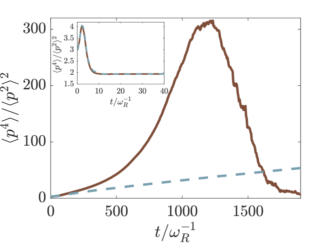
Figure 6: Kurtosis $\mathcal{K}=\langle p^{4}\rangle/\langle p^{2}\rangle^{2}$ as a function of time for the dynamics of Fig. LABEL:tempcomparison (a). The inset shows the kurtosis for the parameters as in Fig. LABEL:tempcomparison (c): Both curves relax to approximately the same value $\mathcal{K}\approx 2$.

III Local mean-field model

We now analyse the dynamics in the regime where the dipoles have synchronized, corresponding to the stage where the correlations $\langle X^{\dagger}X\rangle$ have built up. We perform our study by means of a mean-field approximation, namely, by assuming

$$\langle\hat{\sigma}_{j}\rangle=s_{j}\,,$$ (21)

$$\langle\hat{\sigma}^{z}_{j}\rangle=z_{j}\,,$$ (22)

where $s_{j},z_{j}$ are scalars. This consists of approximating $\langle\hat{\sigma}_{j}^{{\dagger}}\hat{\sigma}_{i}\rangle\approx s_{j}^{*}s_{i}$ for $i\neq j$. Within this treatment, the synchronization order parameter reads

$$X=\langle\hat{X}\rangle=\sum_{j=1}^{N}s_{j}\cos(kx_{j})/N\,.$$ (23)

It is worth emphasizing that we keep the correlations between the internal and the external degrees of freedom, but assume that particle-particle correlations are of mean-field type.

In the mean-field approximation Eqs. (10) and (11) take the form

$$\frac{ds_{j}}{dt}= -\frac{w}{2}s_{j}-\frac{N\Gamma_{C}}{2}i\alpha^{*}X\cos(kx_{j})z_{j},$$ (24)

$$\frac{dz_{j}}{dt}= w(1-z_{j})+2N\Gamma_{C}\mathrm{Im}\left\{\alpha X^{*}s_{j}\right\}\cos(kx_{j}),$$ (25)

where the noise due the incoherent pump is neglected. The corresponding mean-field equations for the external degrees of freedom read:

$$\frac{dx_{j}}{dt}= \frac{p_{j}}{m},$$ (26)

$$\frac{dp_{j}}{dt}= -\hbar k\sin(kx_{j})N\Gamma_{C}\mathrm{Re}\left\{\alpha X^{*}s_{j}\right\}\,,$$ (27)

where the force is the adiabatic component, Eq. (18), and consistent with the mean-field treatment we have discarded cavity shot noise.

III.1 Comparison between mean-field and semiclassical model

We now test the predictions of the mean-field equations by comparing the mean-field dynamics with ones obtained integrating the semiclassical equations, Eqs. (10), (11), and (17). Since the mean-field treatment should more faithfully reproduce the full dynamics for increasing number of particles, we perform simulations for $N=100$ and $N=1000$ particles. In doing so we rescale the coupling strength $g$ so to keep $Ng^{2}$ and thus $N\Gamma_{C}$ constant (compare with Eq. (12)). This implies that the upper synchronization threshold, $w=N\Gamma_{C}$ Meiser:2010:1 , is a constant for this thermodynamics limit, while the lower threshold $w=\Gamma_{C}$ Meiser:2010:1 in this case scales with $1/N$ and thus vanishes for $N\to\infty$.

Figure LABEL:N100mean displays the dynamics of $\langle p^{2}(t)\rangle$ predicted by the semiclassical model (solid line) and by the mean-field model (dashed lines) for $\langle p^{2}(0)\rangle=5\,(\hbar k)^{2}$. The two curves qualitatively agree. Moreover, their behaviour at short times almost coincides and the time interval over which this occurs increases with $N$. A striking difference is the small frequency oscillation, which seems to solely characterize the mean-field dynamics. However, this oscillation becomes visible at time scales at which the mean-field and the semiclassical dynamics start to be quantitatively distinct. The fast oscillations, instead, are also reproduced by the semiclassical equations at $N=1000$. They are also visible in the dynamics of the expectation value of $\langle\hat{X}^{{\dagger}}\hat{X}\rangle$, as shown in Fig. LABEL:N1000mean. We note that the mean-field and full semiclassical dynamics predict approximately the same stationary values of the correlations.

Figure 9 displays the spectral analysis of the two curves in Fig. LABEL:N1000mean(b). In detail, it illustrates the Laplace transform $S(i\omega)$, defined as:

$$S(i\omega)=\int_{0}^{\infty}e^{i\omega t}\left(\langle\hat{X}^{{\dagger}}\hat{X}\rangle(t)-\langle\hat{X}^{{\dagger}}\hat{X}\rangle_{\text{st}}\right)dt\,,$$ (28)

where $\langle\hat{X}^{{\dagger}}\hat{X}\rangle_{\text{st}}=\lim_{t\to\infty}\langle\hat{X}^{{\dagger}}\hat{X}\rangle(t)$. The spectrum of the mean-field data (dashed-dotted curve) and of the data predicted by the semiclassical model (solid curve) exhibits two sidebands at $\omega\simeq\pm 3\omega_{R}$, which we attribute to the oscillations in the potential confining the atoms (see next section). The mean-field simulations predict also two low frequency sidebands at a frequency of the order of a fraction of the recoil frequency, which correspond to the slow oscillations observed in Fig. LABEL:N1000mean(b).

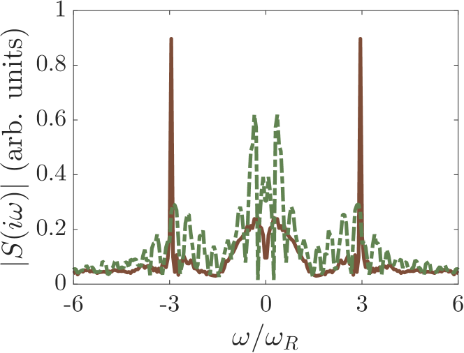
Figure 9: Absolute value of the Laplace transform $S(i\omega)$, Eq. (28), in arbitrary units and as a function of $\omega$ (in units of $\omega_{R}$) for the curves in Fig. LABEL:N1000mean(b). The Laplace transform is evaluated over the same time interval as in Fig. LABEL:N1000mean(b).

III.2 Dynamics at the asymptotic limit

Using the mean-field model we now investigate the dynamics at the asymptotic limit. In particular, we assume that the atoms are sufficiently cold so that at this stage $T_{i}\gg T_{e}$. It is therefore justified to adiabatically eliminate the internal degrees of freedom from the equations of motion of the atoms’ external variables. The procedure is detailed in Appendix C and leads to the stationary values $s_{j}^{(0)}$ and $z_{j}^{(0)}$, which read

$$s_{j}^{(0)}= \frac{\xi(x_{j})}{1+2|\xi(x_{j})|^{2}},$$ (29)

$$z_{j}^{(0)}= \frac{1}{1+2|\xi(x_{j})|^{2}},$$ (30)

and thus depend on the atomic position $x_{j}$ through the quantity

$$\xi(x_{j})=\frac{N\Gamma_{C}}{w}X\cos(kx_{j})\,.$$ (31)

This quantity is proportional to the ratio $N\Gamma_{C}\cos(kx_{j})/w$. It plays an analogous role to the saturation parameter in the dynamics of a driven dipole CohenTannoudji:Book , but its source is of a completely different nature: it depends on the synchronization order parameter $X$, which is found by solving self-consistently the equation

$$\frac{1}{N}\sum_{j=1}^{N}\frac{|\xi(x_{j})|^{2}}{1+2|\xi(x_{j})|^{2}}=\frac{N\Gamma_{C}}{w}|X|^{2}\,.$$ (32)

Concise solutions, which are limiting cases, can be found by assuming that the atoms are tightly confined in a lattice, thereby fixing $\cos(kx_{j})=\pm\delta$. For $\delta=0$, for instance, the only solution is $X=0$. For $\delta\neq 0$, instead, one finds

$$|X|^{2}=\frac{w}{2N\Gamma_{C}}\left(1-\frac{w}{\delta^{2}N\Gamma_{C}}\right)\,.$$ (33)

From this equation it follows that $|X|^{2}=0$ both when $w=0$ and also when $w\geq N\Gamma_{C}\delta^{2}$, namely when $w$ takes the value of the upper synchronization threshold for the corresponding configuration. In particular, the upper synchronization threshold is maximum when $\delta=1$, which corresponds to the value reported in Ref. Meiser:2010:1 .

When instead the atoms are uniformly distributed over the cavity wavelength, Eq. (32) can be recast in the form

$$\frac{N\Gamma_{C}}{w}\frac{1}{2\pi}\int_{0}^{2\pi}d\theta\frac{\cos^{2}\theta}{1+2(N\Gamma_{C}/w)^{2}|X|^{2}\cos^{2}\theta}=1\,.$$ (34)

By using

$$\frac{1}{2\pi}\int_{0}^{2\pi}d\theta\frac{\cos^{2}\theta}{1+2(N\Gamma_{C}/w)^{2}|X|^{2}\cos^{2}\theta}$$

$$=\frac{1}{1+2(N\Gamma_{C}/w)^{2}|X|^{2}+\sqrt{1+2(N\Gamma_{C}/w)^{2}|X|^{2}}}\,,$$

we get

$$|X|^{2}=\frac{w}{2N\Gamma_{C}}\left(1-\frac{w}{N\Gamma_{C}}\left(\frac{1}{2}+\sqrt{\frac{N\Gamma_{C}}{w}+\frac{1}{4}}\right)\right)\,.$$ (35)

From Eq. (35) one obtains that the upper synchronization threshold for particles that are homogeneously distributed over the cavity wavelength is given by $w=N\Gamma_{C}/2$.

We now use this result to determine the spatial dependence of the dipole moment $s_{j}^{(0)}$ and of the population inversion $z_{j}^{(0)}$. These two quantities are plotted in Fig. LABEL:sz(a) and (b), respectively, where we have used the definition $s_{j}^{(0)}\to s(x)$ ($z_{j}^{(0)}\to z(x)$) in the continuum limit. We observe that at the nodes of $\cos(kx)$ the polarization $s(x)$ changes its sign where the population inversion is maximum. In turn, the population inversion is minimal close to the antinode where the polarization reaches its maximum absolute value. If one associates a well-defined magnetic moment to the two electronic states, then the resulting behaviour corresponds to an effective anti-ferromagnetic order.

III.3 Effective Hamiltonian

In the adiabatic limit, where one neglects retardation effects in the coupled dynamics between spin and center-of-mass motion, it is possible to derive an effective Hamiltonian for the atomic external variables. For this purpose we use Eqs. (29) and (30) in Eq. (27) to obtain:

$$\dot{p}_{j}=-\hbar kw\frac{\Delta}{\kappa/2}\tan(kx_{j})\frac{|\xi(x_{j})|^{2}}{1+2|\xi(x_{j})|^{2}}\,.$$

For $N\gg 1$ we can write this equations as $\dot{p}_{j}=-\partial V_{\mathrm{eff}}/\partial x_{j}$ where $V_{\mathrm{eff}}$ is an effective potential of the form:

$$V_{\mathrm{eff}}=-\sum_{j=1}^{N}\frac{\hbar w}{4}\frac{\Delta}{\kappa/2}\log\left(1+2|\xi(x_{j})|^{2}\right)\,.$$ (36)

The corresponding mean-field Hamiltonian, $H_{\mathrm{mean}}$, reads

$$H_{\mathrm{mean}}=\frac{p^{2}}{2m}-\frac{\hbar w}{4}\frac{\Delta}{\kappa/2}\log\left(1+2|\xi(x)|^{2}\right).$$ (37)

The potential minima are at the positions $x$ where $\cos(kx)=\pm 1$. At these points the atoms would be trapped should their asymptotic temperature be smaller than the potential depth $-\hbar\Delta w/(2\kappa)\log(1+2N\Gamma_{C}|X|_{1}^{2}/w)$ (here $|X|_{1}$ is the synchronization order parameter when the atoms are confined at $\cos(kx)=\pm 1$). Correspondingly, the atoms would form an antiferromagnetic spin chain, where the spins swap their orientation so to keep $s_{j}\cos(kx_{j})=1$. In order to verify whether this is the stationary state of the synchronization dynamics, one needs first to determine the asymptotic temperature. Part of this analysis is performed in the next section, where we determine the friction force due to the non-adiabatic coupling with the internal degrees of freedom.

III.4 Dissipative mean-field dynamics

Retardation effects in the dynamics of the spins following the motion give rise to friction. The steady state results from the interplay between the friction and the dispersive force due to the effective potential. We now determine the friction forces in the last cooling stage. For this purpose we perform an expansion of the spin variables including terms to first order in the small parameter ${\mathcal{R}}_{\rm Doppler}/w$:

$$s= s^{(0)}+\frac{kp}{mw}s^{(1)}\,,$$

$$z= z^{(0)}+\frac{kp}{mw}z^{(1)}\,.$$

We then use the prescription $d/dt\to\partial/\partial t+p/m\partial/\partial x$ in Eqs. (24) and (25) and determine the corresponding stationary state (see Appendix D for details).

The friction force is the component of the force in Eq. (27) that depends on the retarded component,

$$F_{\mathrm{ret}}=-(\hbar k/m)p\sin(kx)N\Gamma_{C}\mathrm{Re}\left\{\alpha X^{*}s^{(1)}\right\}\,,$$

and takes the form

$$F_{\mathrm{ret}}=-8\omega_{R}p\frac{|\xi(x)|^{2}\tan^{2}(kx)}{(1+2|\xi(x)|^{2})^{3}}\frac{\Delta}{\kappa/2}\mathcal{F}_{\Delta}(|\xi(x)|^{2})$$ (38)

with

$$\mathcal{F}_{\Delta}(|\xi(x)|^{2})=\frac{{1-2|\xi(x)|^{2}}}{1+\left(\frac{\Delta}{\kappa/2}\right)^{2}}-2|\xi(x)|^{4}\,.$$

This equation shows that the friction force depends on the atomic position. It vanishes at the minima of the mean-field potential, where $\sin(kx)=0$, but tends to pull out the atoms from these points, being positive about $x=n\pi/k$ for $\Delta>0$. The friction coefficient is instead negative for values of $\zeta(x)$ such that

$$|\xi(x)|^{2}\leq\frac{1}{2|\alpha|^{2}}\left(\sqrt{2|\alpha|^{2}+1}-1\right)\,.$$ (39)

The equality holds at the positions $x_{0}$, where the force changes sign. Hence, at the positions $x$ where $\cos^{2}(kx)<\cos^{2}(kx_{0})$ the friction force is negative. Remarkably, these positions are close to the maxima of the mean-field potential.

Figure LABEL:phasespaceplots(a) displays the trajectories in phase space at steady state obtained by integrating the semiclassical equations, while subplot (b) shows the corresponding prediction of the mean-field model. Comparison between subplots (a) and (b) shows that the resulting trajectories form rings centered at $p=0$ and at the points $x=n\pi$ with $n$ denoting any integer number. The rings are connected and the trajectories are indeed close to the separatrix. The separatrix represents the separation of the trajectories where the atoms are bound at the mean-field potential minima from the trajectories where the atoms are unbound. The dashed line indicates in particular the trajectory where the kinetic energy vanishes at the roots $x_{0}$ (namely, where the non-conservative force changes sign). Its energy is given by

$$E_{0}= -\frac{\hbar w}{4}\log\left(1+2|\xi(x_{0})|^{2}\right)\,.$$ (40)

A careful comparison between subplots (a) and (b) shows that cavity shot noise (included in the simulation of (a)) tends to suppress the trajectories with energy below $E_{0}$. Figures LABEL:distributions (a) and (b) report the corresponding momentum and position distributions, respectively. The momentum distribution, Fig. LABEL:distributions (a), is almost flat over the interval $[-p_{0},p_{0}]$, such that $p_{0}^{2}\sim 2mE_{0}$ (these points are indicated by the vertical dashed lines). The semiclassical simulations predict at these specific points two peaks, which are otherwise absent in the mean-field prediction. Instead, mean field and semiclassical simulations deliver very similar position distributions, as shown in Fig. LABEL:distributions (b). Here, the two peaks of the distribution are located about the positions $x_{0}$ where the non-conservative force vanishes.

III.5 Asymptotic temperature

We now estimate the asymptotic temperature by means of the fluctuation-dissipation theorem. The validity of the theorem is limited, since the stationary momentum distribution is not thermal, but allows us to gain insight into the dependence of the momentum distribution on the physical parameters. In what follows we extract the friction coefficient $\gamma$ from the force in Eq. (38):

$$\gamma(x)=8\omega_{R}\frac{|\xi(x)|^{2}\tan^{2}(kx)}{(1+2|\xi(x)|^{2})^{3}}\frac{\Delta}{\kappa/2}\mathcal{F}_{\Delta}(|\xi(x)|^{2})\,.$$ (41)

The calculations for the diffusion coefficients include spin noise due to the incoherent pump, their derivation is involved and reported in Appendix E. The resulting diffusion coefficient $D(x)$ is given in Eq. (57). The final width of the momentum distribution is found after integrating $D(x)$ and $\gamma(x)$ over the asymptotic atomic spatial density distribution, which for convenience we assume to be uniform. Denoting by $\bar{D}$ and $\bar{\gamma}$ the corresponding average values, we obtain

$$\langle p^{2}\rangle_{\infty}=\frac{\bar{D}}{\bar{\gamma}}\,,$$ (42)

where $\langle p^{2}\rangle_{\infty}=\lim_{t\to\infty}\langle p^{2}(t)\rangle$. Figure LABEL:temperature(a) displays the ratio of Eq. (42) as a function of the pump rate $w$ and for $\Delta=\kappa/2$. The minimal width is reached at a value between $w=N\Gamma_{C}/10$ and $w=N\Gamma_{C}/2$. For $w=N\Gamma_{C}/2$, in particular,

$$\frac{\langle p^{2}\rangle_{\infty}}{2m}=\frac{\hbar w}{8}=\frac{\hbar N\Gamma_{C}}{16}\,.$$

Figure LABEL:temperature(b) shows the value of the pump rate which minimizes the momentum width as a function of $\Delta$. The corresponding temperature is shown as a function of $\Delta$ in subplot (c) and is minimized at $\Delta\approx\kappa/2$. The results suggest that lower temperatures can be reached by decreasing $N\Gamma_{C}$ (as long as this value is larger than the recoil frequency, consistently with the semiclassical treatment here applied).

III.6 Discussion

The setup we analyse in this work is the same as the one discussed in Ref. Salzburger:2006 , nevertheless the studies in those papers focus on different parameter regimes which lead to substantially different dynamics. These works predict lasing as well as spatial localization of the atoms in steady state when the atoms are incoherently pumped from the side. The model of Ref. Salzburger:2006 , in particular, focuses on the dynamics of an atomic ensemble. It includes spontaneous emission and assumes that the rate of the incoherent pump is the largest parameter of the dynamics. With this choice population inversion is achieved.

A key point is that the faster time scale of the dynamics in Ref. Salzburger:2004 ; Salzburger:2005 ; Salzburger:2006 is determined by the pump rate and spontaneous decay. For this reason the regime is reached where the atomic internal degrees of freedom follow adiabatically the coupled dynamics of the external and of the resonator degrees of freedom. This is warranted when the atoms are localized in the antinodes of the cavity standing wave. This choice justifies the approximation of discarding terms such as $\langle\hat{\sigma}^{{\dagger}}_{j}\cos(kx_{j})\hat{\sigma}_{i}\cos(kx_{i})\rangle$ for $i\neq j$ in their equations (which also means that this regime cannot exhibit synchronization). This assumption leads to the scaling of the intracavity photon number with the number of atoms in the excited state and thus with $N$ (see Appendix F for further details).

In contrast, here we consider the regime in which the cavity decay $\kappa$ sets the fastest time scale. Moreover, we choose the values of the pump rate for which synchronization is expected. As a result, the dynamics we predict is intrinsically due to collective effects, since it is dominated by mean-field correlations $\langle\hat{X}^{{\dagger}}\hat{X}\rangle\approx\langle\hat{X}^{{\dagger}}\rangle\langle\hat{X}\rangle$, thus they are prevailingly described by correlations of each dipole with all others (the corresponding terms are $N(N-1)$). The field, in turn, scales with the synchronization order parameter $X$, and thus the intracavity photon number scales with $N^{2}$. In this sense the regime studied in Refs. Salzburger:2004 ; Salzburger:2005 ; Salzburger:2006 is complementary to the regime analysed in this paper.

Finally, both models, the one of Ref. Salzburger:2006 and our model, predict stationary momentum distributions whose width is not determined by the width of the resonator. In our model, in particular, the lower bound is determined by the collective linewidth $N\Gamma_{C}$ and is ultimately bound by the recoil energy in order to keep the treatment consistent with the semiclassical approximation.

IV Conclusions

In this manuscript we have analysed the semiclassical dynamics of the atomic external degrees of freedom in the parameter regime where the dipoles synchronize. We have shown that the large friction forces predicted in Ref. Xu:2016 are accompanied by the onset of an antiferromagnetic-like order, where internal and external degrees of freedom become correlated.

Minimal temperatures are found when the parameters are chosen so that the pump rate is in the synchronization regime, $w=N\Gamma_{C}/4$. In this regime the incoherent pump rate indeed determines the asymptotic width of the momentum distribution. Our results suggest the possibility that sub-recoil temperature could be achieved by reducing $N\Gamma_{C}$, as long as this value is larger than the rate of spontaneous decay. Testing this conjecture requires a full quantum mechanical treatment of the dynamics in order to explore the ultimate limits. This is not straight-forward due to the many-body character of the laser-cooling system presented here.

Appendix A Elimination of the cavity field

The formal solution of the Heisenberg-Langevin equation (6) reads

$$\hat{a}(t)= e^{\left(-i\Delta-\frac{\kappa}{2}\right)t}\hat{a}(0)-i\frac{g}{2}\int_{0}^{t}d\tau e^{-\left(i\Delta+\frac{\kappa}{2}\right)(t-\tau)}\sum_{j=1}^{N}\cos(k\hat{x}_{j}(\tau))\hat{\sigma}_{j}(\tau)+\sqrt{\kappa}\int_{0}^{t}d\tau e^{-\left(i\Delta+\frac{\kappa}{2}\right)(t-\tau)}\hat{a}_{\text{in}}(\tau)\,,$$ (43)

with $\hat{a}(0)$ the operator at time $t=0$. To eliminate the cavity field we have to substitute the operator $\hat{a}(t)$ and $\hat{a}^{{\dagger}}(t)$ in the Heisenberg-Langevin equations for the atomic degrees of freedom (Eqs. (3), (4), (5)) with an averaged field

$$\bar{\hat{a}}(t)=\frac{1}{\Delta t}\int_{t}^{t+\Delta t}d\tau\hat{a}(\tau),$$

where we average over the time interval $\Delta t$. If we now assume that $T_{C}\ll\Delta t\ll T_{e}$ and use the general expression in Eq. (43) we derive

$$\bar{\hat{a}}(t)\approx\frac{-i\frac{Ng}{2}\hat{X}}{\frac{\kappa}{2}+i\Delta}-\frac{-i\frac{Ng}{2}\frac{d}{dt}\hat{X}}{\left(\frac{\kappa}{2}+i\Delta\right)^{2}}+\hat{\mathcal{F}}(t)\,,$$ (44)

with $\hat{X}$ the synchronization order parameter, given in Eq. (8). We have introduced an effective Gaussian noise defined on the time scale of the atomic dynamics, which reads

$$\hat{\mathcal{F}}(t)=\sqrt{\kappa/\left(\left(\frac{\kappa}{2}\right)^{2}+\Delta^{2}\right)}\bar{\hat{a}}_{\text{in}}(t)\,,$$ (45)

with

$$\bar{\hat{a}}_{\text{in}}(t)=\frac{1}{\Delta t}\int_{t}^{t+\Delta t}d\tau\hat{a}_{\text{in}}(\tau)\,.$$

The time derivative of $\hat{X}$ in Eq. (44) contains the non-adiabatic corrections to the cavity field, as is visible when explicitly evaluating its form:

$$\frac{d}{dt}\hat{X}= \frac{1}{N}\sum_{j=1}^{N}\cos(k\hat{x}_{j})\frac{d}{dt}\hat{\sigma}_{j}+\frac{1}{N}\sum_{j=1}^{N}\frac{d}{dt}\left(\cos(k\hat{x}_{j})\right)\hat{\sigma}_{j}\,.$$

Appendix B Numerical simulations of the semiclassical equations

In order to perform the integration of Eqs. (10), (11) we perform a second-order cumulant expansion and simulate the matrix $(\langle\hat{\sigma}_{j}^{{\dagger}}\hat{\sigma}_{l}\rangle)_{1\leq j,l\leq N}$ with

$$\frac{d}{dt}\langle\hat{\sigma}_{j}^{{\dagger}}\hat{\sigma}_{j}\rangle= w(1-\langle\hat{\sigma}_{j}^{{\dagger}}\hat{\sigma}_{j}\rangle)$$

$$+N\Gamma_{C}\mathrm{Im}\left(\alpha\left\langle\hat{X}^{{\dagger}}\hat{\sigma}_{j}\right\rangle\right)\cos(kx_{j})\,,$$ (46)

and for $l\neq j$

$$\frac{d}{dt}\langle\hat{\sigma}_{j}^{{\dagger}}\hat{\sigma}_{l}\rangle\approx -\bigg{\{}w+\Gamma_{C}(i\alpha)\cos^{2}(kx_{j})\langle\hat{\sigma}_{j}^{{\dagger}}\hat{\sigma}_{j}\rangle$$

$$+\Gamma_{C}(i\alpha)^{*}\cos^{2}(kx_{l})\langle\hat{\sigma}_{l}^{{\dagger}}\hat{\sigma}_{l}\rangle\bigg{\}}\langle\hat{\sigma}_{j}^{{\dagger}}\hat{\sigma}_{l}\rangle$$

$$+N\frac{\Gamma_{C}}{2}(i\alpha)\cos(kx_{j})(2\langle\hat{\sigma}_{j}^{{\dagger}}\hat{\sigma}_{j}\rangle-1)\langle\hat{X}^{{\dagger}}\hat{\sigma}_{l}\rangle$$

$$+N\frac{\Gamma_{C}}{2}(i\alpha)^{*}\cos(kx_{l})(2\langle\hat{\sigma}_{l}^{{\dagger}}\hat{\sigma}_{l}\rangle-1)\langle\hat{\sigma}_{j}^{{\dagger}}\hat{X}\rangle\,.$$ (47)

The simulations are performed with $N=100$ particles, the data correspond to the average taken over $1000$ trajectories. The initial state is a thermal distribution at a fixed temperature $T$ that is spatially homogeneous, with all atoms are prepared in the excited state:

$$\hat{\rho}_{0}=C\Pi_{j=1}^{N}\exp\left(-\beta\frac{p_{j}^{2}}{2m}\right)\otimes_{j=1}^{N}|e\rangle_{j}\langle e|\,.$$ (48)

Here $C$ is a normalization constant and $\beta=(k_{\text{B}}T)^{-1}$ with the Boltzmann constant denoted by $k_{\text{B}}$.

Appendix C Adiabatic elimination of the internal degrees of freedom in the mean-field model

In order to eliminate the internal degrees of freedom we observe that Eqs. (24),(25) are invariant under the transformation $s_{j}\to\tilde{s}_{j}=s_{j}e^{-i\omega_{0}t}$. Performing this transformation Eqs. (24),(25) take the form

$$\frac{ds_{j}}{dt}= \left(i\omega_{0}-\frac{w}{2}\right)s_{j}-i\frac{N\Gamma_{C}}{2}\alpha^{*}X\cos(kx_{j})z_{j},$$ (49)

$$\frac{dz_{j}}{dt}= w(1-z_{j})+2N\Gamma_{C}\mathrm{Im}\left\{\alpha X^{*}s_{j}\right\}\cos(kx_{j}).$$ (50)

We determine the stationary state by finding $\omega_{0}$ self consistently. For the stationary values $s_{j}^{(0)}$ and $z_{j}^{(0)}$ of Eqs. (49), (50), we find

$$s_{j}^{(0)}=\frac{N\Gamma_{C}\alpha^{*}}{2\omega_{0}+iw}X\cos(kx_{j})z_{j}^{(0)}.$$

We apply this result to determine the synchronization order parameter by using the expression

$$X=\sum_{j=1}^{N}s_{j}^{(0)}\cos(kx_{j})=\frac{N\Gamma_{C}\alpha^{*}}{2\omega_{0}+iw}X\sum_{j=1}^{N}\cos^{2}(kx_{j})z_{j}^{(0)}\,.$$

The latter can be recast in the form

$$\frac{N\Gamma_{C}\alpha^{*}}{2\omega_{0}+iw}\sum_{j=1}^{N}\cos^{2}(kx_{j})z_{j}^{(0)}=1\,.$$ (51)

This expression leads to the condition $N\Gamma_{C}\alpha^{*}/(2\omega_{0}+iw)\in\mathbb{R}$, which is valid providing that

$$\omega_{0}=\frac{w\Delta}{\kappa}\,.$$ (52)

We numerically checked this result by calculating $\cos(\mathrm{arg}(X))$ using mean-field simulations, see Fig. LABEL:Xoscillation (a). It was observed that $X$ oscillates with a well defined frequency, as visible in the Laplace transform of the signal, see Fig. LABEL:Xoscillation (b). For the considered parameters $w/2\approx 5\omega_{R}$.

With this result for $\omega_{0}$ it is possible to obtain the stationary states $s_{j}^{(0)}$ and $z_{j}^{(0)}$ in Eqs. (29) and (30), respectively.

Appendix D Calculation of the friction force due to the coupling with the spins

To calculate retardation effects in the elimination of the spins we replace $d/dt\to\partial/\partial t+p/m\partial/\partial x$ and identify the stationary state with

$$s= s^{(0)}+\frac{p}{m}s^{(1)}\,,$$

$$z= z^{(0)}+\frac{p}{m}z^{(1)}\,.$$

We do not use the index $j$, instead we employ $x$ and $p$ since the whole approach is valid for all particles when we work in the limit $N\to\infty$. If we now use the equations for $s^{(0)}$ and $z^{(0)}$ in Eqs. (29) and (30), this leads to the following equations for $s^{(1)}$ and $z^{(1)}$

$$\frac{\partial s^{(0)}}{\partial x}= i\frac{w}{2}\alpha^{*}s^{(1)}-i\frac{N\Gamma_{C}}{2}\alpha^{*}X\cos(kx)z^{(1)}\,,$$

$$\frac{\partial z^{(0)}}{\partial x}= -wz^{(1)}+2\mathrm{Im}\left(N\Gamma_{C}\alpha X^{*}s^{(1)}\right)\cos(kx)\,.$$

The solutions are

$$s^{(1)}= \xi(x)z^{(1)}\,,$$

$$+2\frac{k}{w}\frac{1}{i\alpha^{*}}\tan(kx)\xi(x)\frac{2|\xi(x)|^{2}-1}{\left(1+2|\xi(x)|^{2}\right)^{2}},$$

$$z^{(1)}= -\frac{k}{w}\tan(kx)\frac{4|\xi(x)|^{2}}{\left(1+2|\xi(x)|^{2}\right)^{3}}$$

$$+4\frac{k}{w}\frac{1-\left(\frac{\Delta}{\kappa/2}\right)^{2}}{1+\left(\frac{\Delta}{\kappa/2}\right)^{2}}\tan(kx)|\xi(x)|^{2}\frac{2|\xi(x)|^{2}-1}{\left(1+2|\xi(x)|^{2}\right)^{3}}.$$

Appendix E Calculation of the diffusion coefficient

To calculate the diffusion coefficient we use Nienhuis

$$2D=\int_{0}^{\infty}d\tau\bigg{(} \frac{1}{2}\left\langle F(0)F(\tau)+F(\tau)F(0)\right\rangle_{\hat{\rho}_{st}}$$

$$-\left\langle F(0)\right\rangle_{\hat{\rho}_{st}}\left\langle F(\tau)\right\rangle_{\hat{\rho}_{st}}\bigg{)}\,,$$ (53)

where the force

$$F(\tau)=\frac{\hbar k}{2}\sin(kx)w\xi^{*}\hat{\sigma}(\tau)+\mathrm{H.c.}$$

is obtained after adiabatic elimination of the cavity (see Eq. (18)). The expectation values are calculated with the stationary density matrix $\hat{\rho}_{\mathrm{st}}$ and $\left\langle\,.\,\right\rangle_{\hat{\rho}_{st}}=\mathrm{Tr}_{i}\left(\,.\,\hat{\rho}_{\mathrm{st}}\right)$ where $\mathrm{Tr}_{i}$ is the trace over the internal degrees of freedom. As we can see in Eqs. (10), (11) the motion of $\hat{\sigma}$, $\hat{\sigma}^{{\dagger}}$, and $\hat{\sigma}^{z}$ is coupled. We define the vector

$$v= \begin{pmatrix}\hat{\sigma}\\ \hat{\sigma}^{{\dagger}}\\ \hat{\sigma}^{z}\end{pmatrix}\,,$$

and write the equations of motion for the spins as

$$\frac{dv}{dt}= \Omega v+b+\mathcal{S}\,,$$ (54)

where the matrix $\Omega$ is defined as

$$\Omega= \begin{pmatrix}i\frac{w}{2}\alpha^{*}&0&-i\frac{w}{2}\alpha^{*}\xi\\ 0&-i\frac{w}{2}\alpha&i\frac{w}{2}\alpha\xi^{*}\\ -iw\alpha\xi^{*}&iw\alpha^{*}\xi&-w\end{pmatrix}\,,$$

and the vector $b$ reads

$$b= \begin{pmatrix}0\\ 0\\ w\end{pmatrix}\,.$$

The noise $\mathcal{S}(\tau)=(S^{-}(\tau)\,\,S^{+}(\tau)\,\,S^{z}(\tau))^{T}$ is defined by

$$\left\langle\mathcal{S}(\tau)\mathcal{S}^{T}(\tau^{\prime})\right\rangle= \begin{pmatrix}0&0&0\\ 1&0&-2\langle\hat{\sigma}^{{\dagger}}(\tau^{\prime})\rangle_{\hat{\rho}_{st}}\\ -2\langle\hat{\sigma}(\tau^{\prime})\rangle_{\hat{\rho}_{st}}&0&2(1-\langle\hat{\sigma}^{z}(\tau^{\prime})\rangle_{\hat{\rho}_{st}})\end{pmatrix}\delta(\tau-\tau^{\prime})\,.$$

The formal solution of Eq. (54) is

$$v(\tau)=e^{\Omega\tau}v+(e^{\Omega\tau}-1)\Omega^{-1}b+\int_{0}^{\tau}d\tau^{\prime}e^{\Omega(\tau-\tau^{\prime})}\mathcal{S}(\tau^{\prime})\,.$$ (55)

If we apply the limit $\tau\to\infty$ for Eq. (55) we get the stationary states for $\hat{\sigma}$, $\hat{\sigma}^{{\dagger}}$, and $\hat{\sigma}^{z}$ which define the stationary density matrix

$$\hat{\rho}_{\mathrm{st}}=\begin{pmatrix}\frac{1+|\xi|^{2}}{1+2|\xi|^{2}}&\frac{\xi^{*}}{1+2|\xi|^{2}}\\ \frac{\xi}{1+2|\xi|^{2}}&\frac{|\xi|^{2}}{1+2|\xi|^{2}}\end{pmatrix}\,.$$ (56)

If we now use the general solution (Eq. (55)) together with the density operator in Eq. (56) to calculate the diffusion coefficient (Eq. (53)) we obtain

$$2D= \frac{(\hbar k)^{2}}{2}w\tan^{2}(kx)|\xi|^{2}\left(1+\frac{2\left(\frac{\Delta_{c}}{\kappa/2}\right)^{2}|\xi|^{2}}{1+2|\xi|^{2}}-2\frac{\left(\frac{\Delta_{c}}{\kappa/2}\right)^{2}}{1+\left(\frac{\Delta_{c}}{\kappa/2}\right)^{2}}\frac{|\xi|^{2}}{\left(1+2|\xi|^{2}\right)^{2}}\frac{5+\left(\frac{\Delta_{c}}{\kappa/2}\right)^{2}+4\left(\left(\frac{\Delta_{c}}{\kappa/2}\right)^{2}+1\right)|\xi|^{2}}{1+2|\xi|^{2}}\right)\,.$$ (57)

Appendix F Detailed comparison with the results of Ref. Salzburger:2006

An interesting example highlighting the complementarity of the two approaches is found by comparing the expectation value of population inversion. In the adiabatic limit (in the thermodynamic limit $Ng^{2}=$const) the population inversion we calculate reads

$$\langle z\rangle\approx\left\langle\frac{1}{1+2|\xi(x)|^{2}}\right\rangle\,,$$

which implies that there is always population inversion $\langle z\rangle\geq 0$. Note that if all particles are in the excited state then $\langle z\rangle=1$, thus $X=0$ and the atoms are not synchronized. Hence synchronization requires a non-vanishing expectation value of the dipole. This is not the case for the parameters of Ref. Salzburger:2006 , where the expectation value of the dipole vanishes at steady state.

We now show that also in Ref. Salzburger:2006 all particles are in the excited state if one takes the equations of motion there defined, neglects spontaneous emission and performs the limit $N\to\infty$ with $Ng^{2}=$ constant, taking $\kappa$ as the largest parameter. For this purpose we take the formula for the population inversion $z_{N}$ in Eq. (25) of Ref. Salzburger:2006 , and report it using our notations giving

$$z_{N}= \frac{\kappa w+N\Gamma w-w\sqrt{\left[\kappa+N\Gamma\right]^{2}-4\kappa N\Gamma}}{2N\Gamma w}\,.$$ (58)

We already neglected spontaneous emission $\gamma=0$ and applied the limit $g^{2}\propto N^{-1}$ with $N\to\infty$. In Eq. (58) the frequency $\Gamma$ is the emission rate defined as $\Gamma=wg^{2}/(w^{2}+\Delta^{2})$. From this expression one can verify that when $\kappa$ is chosen to be the largest frequency then $z_{N}=1$.

References

- (1) D. J. Wineland and W. M. Itano, Phys. Rev. A 20, 1521 (1979).
- (2) S. Chu, Rev. Mod. Phys. 70, 685 (1998); C. N. Cohen-Tannoudji, Rev. Mod. Phys. 70, 707 (1998); W. D. Phillips, Rev. Mod. Phys. 70, 721 (1998).
- (3) C. E. Wieman, D. E. Pritchard, and D. J. Wineland, Rev. Mod. Phys. 71, S253 (1999).
- (4) H. J. Metcalf and P. van der Straten, Laser Cooling and Trapping (Springer, New York, 1999).
- (5) M. Aspelmeyer, T. J. Kippenberg, and F. Marquardt, Rev. Mod. Phys. 86, 1391 (2014).
- (6) A. Rayner, N. R. Heckenberg, and H. Rubinsztein-Dunlop, J. Opt. Soc. of Am. B 20, 1037 (2003).
- (7) J. Eschner, G. Morigi, F. Schmidt-Kaler, and R. Blatt, J. Opt. Soc. Am. B 20, 1003 (2003).
- (8) T. Walker, D. Sesko, and C. Wieman, Phys. Rev. Lett. 64, 408 (1990).
- (9) S. Marksteiner, K. Ellinger, and P. Zoller, Phys. Rev. A 53, 3409 (1996).
- (10) Y. Castin, J. I. Cirac, and M. Lewenstein, Phys. Rev. Lett. 80, 5305 (1998).
- (11) J. I. Cirac, M. Lewenstein, and P. Zoller, Europhys. Lett. 35, 647 (1996).
- (12) S. Stellmer, B. Pasquiou, R. Grimm, and F. Schreck, Phys. Rev. Lett. 110, 263003 (2013).
- (13) P. Horak, G. Hechenblaikner, K. M. Gheri, H. Stecher, and H. Ritsch, Phys. Rev. Lett. 79, 4974 (1997).
- (14) V. Vuletic and S. Chu, Phys. Rev. Lett. 84, 3787 (2000).
- (15) H. Ritsch, P. Domokos, F. Brennecke, and T. Esslinger, Rev. Mod. Phys. 85, 553 (2013).
- (16) M. Hosseini, Y. Duan, K. M. Beck, Y.-T. Chen, and V. Vuletic, preprint arXiv:1701.01226.
- (17) P. Domokos and H. Ritsch, Phys. Rev. Lett. 89, 253003 (2002).
- (18) J. K. Asbóth, P. Domokos, H. Ritsch, and A. Vukics, Phys. Rev. A 72, 053417 (2005).
- (19) S. Schütz and G. Morigi, Phys. Rev. Lett. 113, 203002 (2014).
- (20) S. Schütz, S. B. Jäger, and G. Morigi, Phys. Rev. A 92, 063808 (2015).
- (21) T. Salzburger and H. Ritsch, Phys. Rev. Lett. 93, 063002 (2004).
- (22) T. Salzburger, P. Domokos, and H. Ritsch, Phys. Rev. A 72, 033805 (2005).
- (23) T. Salzburger and H. Ritsch, Phys. Rev. A 74, 033806 (2006).
- (24) J. G. Bohnet, Z. Chen, J. M. Weiner, D. Meiser, M. J. Holland, and J. K. Thompson, Nature (London) 484 ,78 (2012).
- (25) M. Xu, S. B. Jäger, S. Schütz, J. Cooper, G. Morigi, and M. J. Holland, Phys. Rev. Lett. 116, 153002 (2016).
- (26) D. Meiser, J. Ye, D. R. Carlson, and M. J. Holland Phys. Rev. Lett. 102, 163601 (2009).
- (27) D. Meiser and M. J. Holland, Phys. Rev. A 81, 033847 (2010).
- (28) C. W. Gardiner and M. J. Collett, Phys. Rev. A 31, 3761 (1985).
- (29) S. Stenholm, Rev. Mod. Phys. 58, 699 (1986).
- (30) For details on the implementation of the stochastic differential equations in a similar setup see S. Schütz, H. Habibian, and G. Morigi, Phys. Rev. A 88, 033427 (2013).
- (31) C. Cohen-Tannoudij, J. Dupont-Roc, G. Grynberg, Atom- Photon Interactions (Wiley, Toronto, 1992).
- (32) G. Nienhuis, P. van der Straten, and S-Q. Shang, Phys. Rev. A 44, 462 (1991).