Document Visualization using Topic Clouds

Abstract

Traditionally a document is visualized by a word cloud. Recently, distributed representation methods for documents have been developed, which map a document to a set of topic embeddings. Visualizing such a representation is useful to present the semantics of a document in higher granularity; it is also challenging, as there are multiple topics, each containing multiple words. We propose to visualize a set of topics using Topic Cloud, which is a pie chart consisting of topic slices, where each slice contains important words in this topic. To make important topics/words visually prominent, the sizes of topic slices and word fonts are proportional to their importance in the document. A topic cloud can help the user quickly evaluate the quality of derived document representations. For NLP practitioners, It can be used to qualitatively compare the topic quality of different document representation algorithms, or to inspect how model parameters impact the derived representations.

1 Introduction

Word clouds (also known as “tag clouds”) are a conventional way to visually represent the words in a document (Rivadeneira et al., 2007). Typically the font size of a word is proportional to its importance in the document. Figure 1 presents a frequency-weighted word cloud in a typical style, generated from a news report about a pharmaceutical company acquisition. The colors of words are randomly selected from a palette, without semantic indications.

One apparent problem of the word cloud is that, as the complexity of the document increases, it soon becomes difficult to read. For instance, Figure 1 only contains 60 words, but a viewer will probably only notice the few largest words, and could not form a “big picture” of the document, as the semantic transition across words are random and abrupt. (Hassan-Montero & Herrero-Solana, 2006) proposed to cluster words according to their semantic relatedness, and draw differnt clusters in different lines. This alleviates the unorganized nature of the word cloud to certain extent.

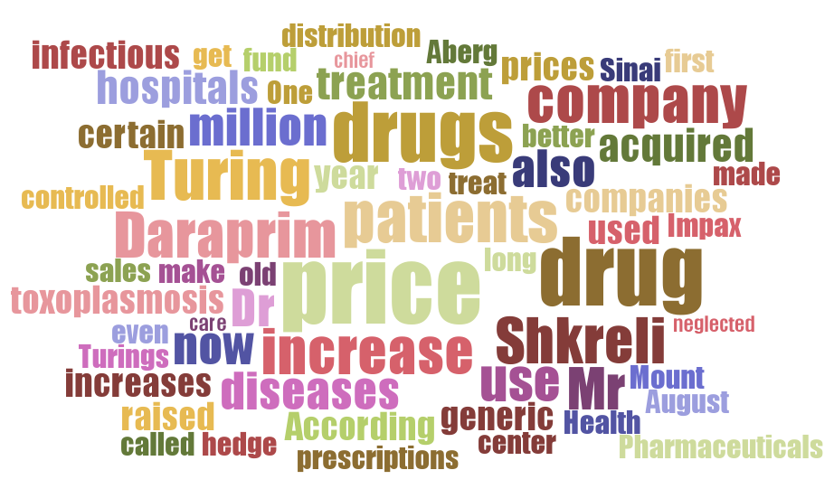
Figure 1: A typical word cloud generated from a news report, containing the 60 most frequent words (stop-words are removed).

The advent of distributed representations (“embeddings”) of words and text has led to an evolution of Natural Language Processing (Collobert et al., 2011; Mikolov et al., 2013). Embedding methods map words and text into continuous feature vectors in a low-dimensional space, making them easy to process by downstream machine learning algorithms. Recently, a few methods have been proposed to map documents into a set of embeddings (Le & Mikolov, 2014; Liu et al., 2015; Das et al., 2015; Batmanghelich et al., 2016; Li et al., 2016). Most of these works derive embeddings that are topical, i.e., each embedding defines a topic (a distribution of words) of the document. Compared to conventional topic models (Blei et al., 2003), these methods derive more coherent topics by exploiting semantic relatedness encoded in pretrained word embeddings; moreover, some of them, e.g. (Li et al., 2016), are able to derive topic embeddings based on only one document.

Topic embeddings, along with the corresponding topic proportions, represent the semantics of a document in a refined granularity. Visualizing the topic embddings, or the corresponding topics, can help users quickly perceive the main concepts in a document. However there are multiple topics, each containing multiple words, and words/topics differ in their prominence. It is challenging to represent the topics in a form that is both visually organized, and also manifests the different prominence of words/topics. To this end, we propose Topic Cloud, which is a pie chart consisting of topic slices, where each slice contains important words in this topic. The relative prominence of words/topics are made explicit by drawing the words/topics in sizes that are proportional to their importance in the document. Figure 2 provides an example of topic clouds.

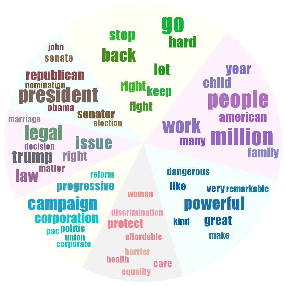
Figure 2: A topic cloud generated from one of Hillary Clinton’s presidential campaign speech.

The topic cloud is an easily recognizable visualization of the topical representation of a document. It helps the user quickly perceive the main concepts in a document. In addition, it also makes it easy for the user to evaluate the quality of derived representations of documents. For NLP practitioners, It can be used to qualitatively compare the topic quality of different document representation algorithms, or to inspect how model parameters impact the derived representations.

The source code of our Topic Cloud implementation is available at https://github.com/askerlee/topiccloud.

2 The Topic Cloud Algorithm

Algorithm 1 Topic cloud generation.

Input: $K$ topics $T=\{t_{1},\cdots,t_{K}\}$, where $t_{k}=p_{k},(w_{k1},q_{k1};\cdots,w_{km},q_{km})$; exponential scaling coefficient $\beta$, thresholds of topic proportion ratio $\mu$ and word importance $\sigma$, maximal and minimal font sizes $f_{\textrm{max}}$,$f_{\textrm{min}}$;

Draw a circle of radius $r$ as the canvas;

Sort all topics in descending order of their proportions $p_{k}$;

Remove all topics $t_{k}$ satisfying $p_{k}<p_{1}/\mu$;

Normalize $p_{k}$ as $p_{k}^{\prime}=\frac{p_{k}^{\beta}}{\sum_{j}p_{j}^{\beta}};$

$q_{\textrm{max}}=\max_{k,i}q_{ki}$;

$a_{0}=270-180\cdot p_{k}^{\prime}$;

for $t_{k}$ in $T$ do

Allocate $t_{k}$ a pie slice with angles in $[a_{0},a_{0}+360\cdot p_{k}^{\prime}]$;

Draw the slice $s_{k}$ with background color $c_{1+i\textrm{ mod }L_{1}}\in\{c_{1},\cdots,c_{L_{1}}\}$, a predefined palette;

Set the base word color in $t_{k}$ as $\textrm{bg}_{k}=d_{1+k\textrm{ mod }L_{2}}\in\{d_{1},\cdots,d_{L_{2}}\}$, another predefined palette;

Sort $w_{k1},\cdots,w_{km}$ in descending order of $q_{ki}$;

Remove all words satisfying $q_{ki}<\sigma$;

for $w_{ki}$ in $t_{k}$ do

Set the font size of $w_{ki}$ as $f_{ki}=f_{\textrm{max}}\cdot(q_{ki}/q_{\textrm{max}})^{\beta}$;

$f_{ki}=\max(f_{ki},f_{\textrm{min}})$;

Compute the bounding box $B_{ki}$ of $w_{ki}$ in font size $f_{ki}$;

repeat

Find all points $S=\{(x_{j},y_{j})\}$ within slice $s_{k}$ that can be used as the upperleft corner of $B_{ki}$, i.e. all points within $B_{ki}$ is unoccupied;

if $S=\phi$ then

$f_{ki}=f_{ki}-1$

end if

until $S\neq\phi$

Randomly pick $(x,y)\in S$;

Let $\textrm{bg}_{k}=\textrm{rgb}(r_{k},g_{k},b_{k})$. Randomly perturb $r_{k},g_{k},b_{k}$ by a random integer in $[-\epsilon,\epsilon]$, and get $\textrm{rgb}(r_{k}^{\prime},g_{k}^{\prime},b_{k}^{\prime})$ as the color of $w_{ki}$;

Draw $w_{ki}$ in $B_{ki}$ at $(x,y)$;

Mark all points in $B_{ki}$ as being occupied;

end for

$a_{0}=a_{0}+360\cdot p_{k}^{\prime}$;

end for

The topic cloud generation algorithm receives a set of topics as the input, where each topic $t_{k}$ is in the form of $p_{k},(w_{k1},q_{k1};\cdots,w_{km},q_{km})$. Here $p_{k}$ is the proportion of $t_{k}$ in the represented document, $m$ is a pre-specified word number threshold, $w_{ki}$ is a word belonging to $t_{k}$, and $q_{ki}$ is its relative importance. As a preprocessing step, we lemmatize all words in each topic. If two words $w_{ki},w_{kj}$ are lemmatized into the same word $w_{ki}^{\prime}$, then their importance is combined as $q_{ki}^{\prime}=q_{ki}+q_{kj}.$

The topic cloud generation algorithm is straightforward, as described in Algorithm 1. For convenience of computation, the 90°  angle is defined at the center bottom of the canvas. We start putting topics clockwise from the center top, i.e. around the 270°  angle.

3 Example Applications

Traditionally, the quality of derived topical representations is usually measured by the model perplexity, or by the Pointwise Mutual Information (PMI) score of the words in the topic against a golden standard. But the perplexity is not intuitive, and the perplexity between different methods may be incomparable. On the other hand, the PMI score is costly to compute.

When we only want to informally evaluate the quality of derived representations, we could resort to qualitative analysis. Qualitatively, the topical representations can be measured in two aspects: 1) whether the words in each major topic is semantically coherent; 2) whether the proportions of topics comply with the following intuitions: the topics in a document are usually sparse, i.e., only a few major topics take most of the proportions, and other topics have minor proportions; on the other hand, topic proportions are usually somewhat uneven (gradually decreasing).

The topic cloud can be used to qualitatively evaluate these two aspects of derived representations. Here we present an application of comparing the performance of two topic embedding methods, followed by an application of tuning a parameter of a topic embedding method.

3.1 Comparison of Topical Representations by K-Means and TopicVec

In this example, the two compared methods are a simple k-means clustering algorithm on the word embeddings and TopicVec (Li et al., 2016). The topic numbers of both methods were set to 10. As the cosine similarity measures the semantic relatedness between embeddings, the metric of k-means was specified as the cosine distance. Before performing k-means, the embedding vectors were normalized. The input document was the pharmaceutical company acquisition news report, the same input of Figure 1.

Figure 3 and 4 present the topic clouds derived by k-means and TopicVec, respectively. For k-means, each cluster was a topic, and the cluster centroid (the average embedding in a cluster) was used as the topic embedding. The topic proportion was defined as the proportion of words in this cluster. Constrained by the limited circle area, only the 6 biggest topics were shown in each topic cloud. In the following, we refer to the center top topic slice as the first topic, which is always the biggest slice.

One can quickly see that in Figure 3, the first two topics (clockwise counted) are coherent, and the remaining 4 topics become increasingly noisy. In contrast, the topics in Figure 4 are generally coherent, with very few noisy words.

By comparing Figure 3 and 4, we can see that topics produced by k-means are more even, with similar sizes; while the topics produced by TopicVec are more disproportionate. The latter agrees better with the intuition of topic sparsity.

In sum, with the help of topic clouds, one can quickly learn that TopicVec derives better topical representations than k-means, both in topic coherence and topic proportions.

Figure 3: The topic cloud derived by k-means.

Figure 4: The topic cloud derived by TopicVec.

3.2 Impact of Parameters on Topics by TopicVec

In this example, we tune an important parameter of TopicVec, i.e., the maximal magnitude $\gamma$ of topic embeddings.

Figure 5 and 6 present the topic clouds derived by TopicVec on the accepted paper list of ICML 2016. $\gamma$ was set to 3 and 5, respectively. In Figure 5, one can quickly find out that all topics except the first one are highly similar, and all topics have similar proportions. In contrast, in Figure 6, words are clustered into different coherent topics, and the topic proportions gradually decrease clockwise. The two topic clouds reveal that $3$ is a poor setting of $\gamma$, and 5 is reasonable.

Figure 5: The topic cloud derived by TopicVec with $\gamma=3$, on the accepted paper list of ICML’16.

Figure 6: The topic cloud derived by TopicVec with $\gamma=5$, on the accepted paper list of ICML’16.

4 Future Work

Our method of Topic Cloud generation is still preliminary. One deficiency of the present method is that, the words within each topic are placed randomly, without considering their semantic relatedness. It would be easier for human to perceive if, within each topic, words are arranged according to their semantic relatedness, i.e. more relevant words are put more closely. Distance preserving dimension reduction methods, such as t-SNE (Van der Maaten & Hinton, 2008) (extension is needed to incorporate boundary and word size constraints), could be adopted to perform a projection from word embeddings within a topic to a pie slice. With such a technique, the drawn topic cloud will be visually more coherent, allowing users to more quickly recognize the concepts in each topic.

References

- Batmanghelich et al. (2016) Batmanghelich, Kayhan, Saeedi, Ardavan, Narasimhan, Karthik, and Gershman, Sam. Nonparametric spherical topic modeling with word embeddings. In Proceedings of the ACL 2016, 2016. Short paper.
- Blei et al. (2003) Blei, David M, Ng, Andrew Y, and Jordan, Michael I. Latent dirichlet allocation. the Journal of machine Learning research, 3:993–1022, 2003.
- Collobert et al. (2011) Collobert, Ronan, Weston, Jason, Bottou, Léon, Karlen, Michael, Kavukcuoglu, Koray, and Kuksa, Pavel. Natural language processing (almost) from scratch. The Journal of Machine Learning Research, 12:2493–2537, 2011.
- Das et al. (2015) Das, Rajarshi, Zaheer, Manzil, and Dyer, Chris. Gaussian lda for topic models with word embeddings. In ACL, 2015.
- Gottron (2009) Gottron, Thomas. Document word clouds: Visualising web documents as tag clouds to aid users in relevance decisions. In Research and Advanced Technology for Digital Libraries, pp. 94–105. Springer, 2009.
- Hassan-Montero & Herrero-Solana (2006) Hassan-Montero, Yusef and Herrero-Solana, Victor. Improving tag-clouds as visual information retrieval interfaces. In International Conference on Multidisciplinary Information Sciences and Technologies, pp. 25–28. Citeseer, 2006.
- Le & Mikolov (2014) Le, Quoc and Mikolov, Tomas. Distributed representations of sentences and documents. In Proceedings of the 31st International Conference on Machine Learning (ICML-14), pp. 1188–1196, 2014.
- Li et al. (2016) Li, Shaohua, Chua, Tat-Seng, Zhu, Jun, and Miao, Chunyan. Generative topic embedding: a continuous representation of documents. In Proceedings of the ACL 2016, 2016.
- Liu et al. (2015) Liu, Yang, Liu, Zhiyuan, Chua, Tat-Seng, and Sun, Maosong. Topical word embeddings. In AAAI, pp. 2418–2424, 2015.
- Mikolov et al. (2013) Mikolov, Tomas, Sutskever, Ilya, Chen, Kai, Corrado, Greg S, and Dean, Jeff. Distributed representations of words and phrases and their compositionality. In Proceedings of NIPS 2013, pp. 3111–3119, 2013.
- Rivadeneira et al. (2007) Rivadeneira, Anna W, Gruen, Daniel M, Muller, Michael J, and Millen, David R. Getting our head in the clouds: toward evaluation studies of tagclouds. In Proceedings of the SIGCHI conference on Human factors in computing systems, pp. 995–998. ACM, 2007.
- Van der Maaten & Hinton (2008) Van der Maaten, Laurens and Hinton, Geoffrey. Visualizing data using t-sne. Journal of Machine Learning Research, 9(2579-2605):85, 2008.