Electromagnetic form factors at large momenta from lattice QCD

Abstract

Accessing hadronic form factors at large momentum transfers has traditionally presented a challenge for lattice QCD simulations. Here we demonstrate how a novel implementation of the Feynman–Hellmann method can be employed to calculate hadronic form factors in lattice QCD at momenta much higher than previously accessible. Our simulations are performed on a single set of gauge configurations with three flavours of degenerate mass quarks corresponding to $m_{\pi}\approx 470\text{ MeV}$. We are able to determine the electromagnetic form factors of the pion and nucleon up to approximately 6 GeV², with results for $G_{E}/G_{M}$ in the proton agreeing well with experimental results.

I Introduction

One of the great challenges of hadron physics is to build consistent and informative pictures of the internal structures of strongly-interacting particles. An important aspect of this endeavour is the calculation of electromagnetic form factors for various baryons and mesons. These encode a description of the distribution of electromagnetic currents in hadrons and are key to describing the extended structure of these composite states.

For most of the second half of the 20^th century, measurements of the electromagnetic form factors of the nucleon were obtained using the Rosenbluth separation technique Rosenbluth (1950) (also e.g. Qattan et al. (2005)). Broadly, these experiments indicated that the electric and magnetic form factors scaled proportionally for $Q^{2}$ up to around 6 GeV², with $\mu_{p}{G_{E}}_{p}/{G_{M}}_{p}\approx 1$. This was later found to be in disagreement with recoil polarisation experiments at Jefferson Lab which showed $\mu_{p}{G_{E}}_{p}/{G_{M}}_{p}$ decreasing approximately linearly for $Q^{2}\gtrsim 0.5\text{ GeV}^{2}$ (see e.g. Jones et al. (2000); Gayou et al. (2002); Punjabi et al. (2005); Puckett et al. (2010, 2012)). This discrepancy is now largely understood through studies of two-photon exchange effects in the Rosenbluth method Guichon and Vanderhaeghen (2003); Blunden et al. (2005). Nevertheless, it is still unknown whether the linear $Q^{2}$ trend continues and crosses zero, or if the fall-off with $Q^{2}$ slows down. Experimental results are as yet unable to obtain precise results at the relevant momentum scales, and so this remains an open question. Resolving the scaling of the form factors in this domain is one of the key physics goals of the upgraded CEBAF at Jefferson Lab.

The large-$Q^{2}$ behaviour of the pion electromagnetic form factor $F_{\pi}$ has proven challenging to probe experimentally — see Refs. Volmer et al. (2001); Horn et al. (2006); Huber et al. (2008) for recent innovative advances. Besides providing information about the electromagnetic structure of the pion, the $Q^{2}$-behaviour of $F_{\pi}$ provides insight into the transition from the soft to the hard regime in QCD (see Chang et al. (2013) for a recent example). Owing to the present limitations, experimental data are unable to reliably discriminate different models describing the transition to the asymptotic domain Horn and Roberts (2016).

Lattice calculations of hadronic form factors have typically focussed on the study of processes at low-momentum transfer (see e.g. Collins et al. (2011); Alexandrou et al. (2011); Shanahan et al. (2014a, b); Green et al. (2014); Capitani et al. (2015)), with only limited studies at large $Q^{2}\gtrsim 3\text{ GeV}^{2}$ Lin et al. (2010); Koponen et al. (2017). There are a variety of reasons that have contributed to the diffculty in accessing high-momentum transfer in lattice QCD. Given that the form factors fall with $Q^{2}$, it is immediately clear that one is attempting to extract a much weaker signal from datasets obtained with finite statistics. Further, in terms of the numerical computation, the signal-to-noise ratio of hadron correlators rapidly deteriorates as the momentum of the state is increased. This had commonly led to the study of 3-point correlators which are projected to zero momentum at the hadron sink. In this case, the possible momentum transfers are limited by the maximum momentum available at the source. With limited statistical signal, it is therefore difficult to assess the degree of excited-state contamination, which can lead to significant systematic uncertainty Lin et al. (2010); Owen et al. (2013); Green et al. (2014); Yoon et al. (2016); Dragos et al. (2016).

In the present work we demonstrate the ability to access high-momentum transfer in hadron form factors on the lattice using an extension of the Feynman–Hellmann theorem to non-forward matrix elements. This builds upon recent applications of the Feynman–Hellmann theorem for hadronic matrix elements in lattice QCD Horsley et al. (2012); Chambers et al. (2014, 2015a, 2015b) — see also Refs. Detmold (2005); Engelhardt (2007); Detmold et al. (2009, 2010); Primer et al. (2014); Freeman et al. (2014); Savage et al. (2016); Bouchard et al. (2016) for similar related techniques. Through the Feynman–Hellmann theorem one relates matrix elements to energy shifts. In the case of lattice QCD this allows one to access matrix elements from 2-point correlators, rather than a more complicated analysis of 3-point functions. This greatly simplifies the process of neutralising excited-state contamination. As described below, the method most naturally works in the Breit frame ($E(\boldsymbol{p}^{\prime})=E(\boldsymbol{p})$) and hence one maximises the momentum transfer for any given accessible state momentum $|{\bf p}|$. Finally, the high degree of correlations in the gauge ensembles makes it possible to extract a weak signal from a relatively noisy state.

II Feynman–Hellmann Methods

To extend the Feynman–Hellmann analysis to non-forward matrix elements, we first consider a simple quantum mechanical situation. The familiar form of the FH theorem reads

$$\mathinner{\dfrac{\partial{}E_{\psi}}{\partial{\lambda}}}=\left\langle\,\psi\,\middle|\,\mathinner{\dfrac{\partial{}H}{\partial{\lambda}}}\,\middle|\,\psi\,\right\rangle\,,$$ (1)

where $E$ is the energy eigenvalue of the state $\psi$. This readily follows from first-order perturbation theory. In the presence of spatially-varying external fields, the conventional theorem requires a slight modification. We consider some first-order perturbation of the Hamiltonian, $H=H_{0}+\lambda V$, which couples to a definite (real) spatial Fourier component

$$\frac{\partial H}{\partial\lambda}\equiv\widetilde{V}_{+}(\boldsymbol{q})=\widetilde{V}(\boldsymbol{q})+\widetilde{V}(-\boldsymbol{q})\,,$$ (2)

defined in terms of the complex Fourier modes $\widetilde{V}(\boldsymbol{q})=\int\mathrm{d}^{3}\boldsymbol{y}\,e^{i\boldsymbol{q}.\boldsymbol{y}}V(\boldsymbol{y})$, for some Hermitian potential $V(\boldsymbol{y})$. The diagonal matrix elements of this operator vanish in the basis of definite momentum eigenstates

$$\langle\boldsymbol{p}|\widetilde{V}_{+}(\boldsymbol{q})|\boldsymbol{p}\rangle=0\,,$$ (3)

and standard perturbation theory would suggest that there is no shift of the energy level at first order in $\lambda$. The exception to this rule is in the case of a degeneracy in the unperturbed eigenstates $E_{0}(\boldsymbol{p})=E_{0}(\boldsymbol{p}\pm\boldsymbol{q})$. The familiar solution in this case is to invoke degenerate perturbation theory where one diagonalises the space of the degeneracy with respect to the applied external potential. The degeneracy condition dictates that one is considering Breit-frame transitions. For demonstrative purposes, we choose the simple case where $\boldsymbol{p}=\pm\boldsymbol{q}/2$ and hence at lowest order in the field strength the system is diagonalised by the states $|\boldsymbol{q}/2\rangle_{\pm}\propto|\boldsymbol{q}/2\rangle\pm|-\boldsymbol{q}/2\rangle$. The corresponding eigenvalues are given by $E_{0}(\boldsymbol{q/2})\pm\lambda\Delta E+\mathcal{O}(\lambda^{2})$, where the energy shift corresponds to the matrix element of interest,

$$\Delta E ={}_{+}\langle\boldsymbol{q}/2|\widetilde{V}_{+}(\boldsymbol{q})|\boldsymbol{q}/2\rangle_{+}=\langle\boldsymbol{q}/2|\widetilde{V}(\boldsymbol{q})|-\boldsymbol{q}/2\rangle\,.$$ (4)

Owing to the discretised spectrum (and momentum) on the lattice, this quantum mechanical argument translates in a straightforward fashion to hadronic matrix elements. In the case of continuous momenta the presence of the periodic potential induces a gap in the dispersion curve, as in conventional band theory.

To implement within a lattice calculation, the Lagrangian is modified to incorporate a spatially-varying external potential

$$\mathcal{L}(y) \to\mathcal{L}(y)+\lambda\left(e^{+i\boldsymbol{q}\cdot\boldsymbol{y}}+e^{-i\boldsymbol{q}\cdot\boldsymbol{y}}\right)\mathcal{O}(y)\,,$$ (5)

where the phase of the exponentials is defined with respect to the location of the hadron source at $\boldsymbol{y}=\boldsymbol{0}$. The symbol $\mathcal{O}$ denotes a quark-bilinear operator and $\lambda$ represents the strength of the external field — which is kept small ensure that the energy response is in the linear regime. Alternatively, one may isolate the linear $\lambda$ dependence of the correlator directly by constructing compound propagators Savage et al. (2016); Bouchard et al. (2016).

To compute connected quark contributions, quark propagators are inverted according the modified action corresponding to Eq. (5) — sea-quark contributions would require new gauge ensembles Chambers et al. (2015b) or an effective reweighting technique. Fourier-projected, hadron correlation functions are defined by

$$C_{\boldsymbol{p}}^{\lambda}(t)=\sum_{\boldsymbol{x}}e^{-i\boldsymbol{p}.\boldsymbol{x}}\,{}_{\lambda}\langle\Omega|\chi(t,\boldsymbol{x})\chi^{\dagger}(0,\boldsymbol{0})|\Omega\rangle_{\lambda}\,,$$ (6)

where subscript $\left|\,\Omega\,\right\rangle_{\lambda}$ is the vacuum of the modified theory. The spectrum can be directly isolated by constructing even and odd linear combinations,

$$C_{\boldsymbol{p},\boldsymbol{p}^{\prime}}^{\lambda\pm}=C_{\boldsymbol{p}}^{\lambda}\pm C_{\boldsymbol{p}^{\prime}}^{\lambda}\,,$$ (7)

of Breit-frame momentum pairs, $\boldsymbol{p}$ and $\boldsymbol{p}^{\prime}(=\boldsymbol{p}+\boldsymbol{q})$. To isolate an energy shift, it is more straightforward to implement the “$+$” combination $C_{\boldsymbol{p},\boldsymbol{p}^{\prime}}^{\lambda+}$ rather than the “$-$” sum, which vanishes in the free-field limit.

Only the Breit-frame pairs will receive an energy shift which is linear in the applied field strength $\lambda$. This energy shift corresponds directly to the hadronic matrix element of interest

$$\left.\mathinner{\dfrac{\partial{}E_{H}(\boldsymbol{p}^{\prime})}{\partial{\lambda}}}\right|_{\lambda=0}=\frac{\left\langle\,H(\boldsymbol{p}^{\prime})\,\middle|\,\mathcal{O}(0)\,\middle|\,H(\boldsymbol{p})\,\right\rangle}{\left\langle\,H(\boldsymbol{p}^{\prime})\,\middle|\,H(\boldsymbol{p}^{\prime})\,\right\rangle}\,,$$ (8)

or similarly for $\boldsymbol{p}\leftrightarrow\boldsymbol{p}^{\prime}$. We have confirmed numerically that non-Breit frame states do not receive a linear energy response, as expected.

III Simulation Details

In the present work, we use an ensemble of 1700 gauge field configurations with $2+1$ flavours of non-perturbatively $O(a)$-improved Wilson fermions and a lattice volume of $L^{3}\times T=32^{3}\times 64$. The lattice spacing $a=0.074(2)\text{ fm}$ is set using a number of singlet quantities Horsley et al. (2013); Bornyakov et al. (2015); Bietenholz et al. (2010, 2011). The clover action used comprises the tree-level Symanzik improved gluon action together with a stout smeared fermion action, modified for the implementation of the FH method Chambers et al. (2014).

We use a single ensemble with hopping parameters, $(\kappa_{l},\kappa_{s})=(0.120900,0.120900)$, which correspond to a pion mass of $\sim 470\text{ MeV}$. To study electromagnetic form factors, quark propagators are calculated with the modified Lagrangian

$$\mathcal{L}(y)\to\mathcal{L}(y)+\left(e^{+i\boldsymbol{q}\cdot\boldsymbol{y}}+e^{-i\boldsymbol{q}\cdot\boldsymbol{y}}\right)\bar{q}(y)\lambda\cdot\gamma q(y)\,,$$ (9)

for multiple values of $\boldsymbol{q}$ as listed in Table 1, where either $\lambda_{2}$ or $\lambda_{4}$ take non-zero values of $1\times 10^{-4}$ or $-1\times 10^{-5}$. Note that we only use the simplest Breit-frame kinematics, $\boldsymbol{p}^{\prime}=-\boldsymbol{p}$. This choice allows us to minimise ${\boldsymbol{p}}^{2}$ for each value of $\boldsymbol{q}^{2}$, and hence minimise the noise in the correlator. As described below, this also projects the nucleon energy shifts directly onto $G_{E}$ or $G_{M}$.

$\boldsymbol{q}$	$\boldsymbol{p}$	$\boldsymbol{p}^{2}$	$Q^{2}$
$(0,0,0)$	$(0,0,0)$	$0$	$0$
$(2,0,0)$	$(1,0,0)$	$1$	$4$
$(2,2,0)$	$(1,1,0)$	$2$	$8$
$(2,2,2)$	$(1,1,1)$	$3$	$12$
$(4,0,0)$	$(2,0,0)$	$4$	$16$
$(4,2,0)$	$(2,1,0)$	$5$	$20$
$(4,2,2)$	$(2,1,1)$	$6$	$24$

Table 1: Momentum insertions and the corresponding Breit-frame momenta used in these calculations, where $\boldsymbol{p}^{\prime}=-\boldsymbol{p}$. Momenta are given in lattice Fourier units of $2\pi/L$.

IV Results

IV.1 Electromagnetic Form Factors of the Nucleon

The (Euclidean) decompositon of the vector current for the individual quark flavour contributions of the nucleon is written in terms of the familiar Dirac and Pauli (${F_{1}}_{q}$ and ${F_{2}}_{q}$) form factors,

$$\left\langle\,N(p^{\prime},s^{\prime})\,\middle|\,\bar{q}(0)\gamma_{\mu}q(0)\,\middle|\,N(p,s)\,\right\rangle=$$

$$\bar{u}(p^{\prime},s^{\prime})\left[\gamma_{\mu}{F_{1}}_{q}(Q^{2})+\frac{\sigma_{\mu\nu}q_{\nu}}{2M_{N}}{F_{2}}_{q}(Q^{2})\right]u(p,s)\,,$$ (10)

where we denote the invariant 4-momentum transfer squared as $Q^{2}=-q^{2}=-{(p^{\prime}-p)}^{2}$. The Sachs electromagnetic form factors are defined by

$${G_{E}}_{q} ={F_{1}}_{q}-\frac{Q^{2}}{{(2M)}^{2}}{F_{2}}_{q}$$ (11)

$${G_{M}}_{q} ={F_{1}}_{q}+{F_{2}}_{q}$$ (12)

For the incident-normal Breit frame ($\boldsymbol{p}^{\prime}=-\boldsymbol{p}$), the temporal and spatial components of the current give rise to energy shifts which directly project out the electric and magnetic form factors respectively,

$$\left.\mathinner{\dfrac{\partial{}E_{N}}{\partial{\lambda_{4}}}}\right|_{\lambda=0} \overset{\boldsymbol{p}^{\prime}=-\boldsymbol{p}}{=}\frac{M_{N}}{E_{N}}{G_{E}}_{q}\,,$$ (13)

$$\left.\mathinner{\dfrac{\partial{}E_{N}}{\partial{\lambda_{i}}}}\right|_{\lambda=0} \overset{\boldsymbol{p}^{\prime}=-\boldsymbol{p}}{=}\frac{{[\hat{\boldsymbol{e}}\times\boldsymbol{q}]}_{i}}{2E_{N}}{G_{M}}_{q}\,,$$ (14)

where $\hat{\boldsymbol{e}}$ is the spin polarisation vector determined by the choice of polarisation direction of the nucleon.

Utilising ratios of correlators with and without the applied external field, we can defined “effective form factors” by appropriate scaling of the effective energy shift $\Delta{E_{N}}_{\text{eff.}}$,

$${{G_{E}}_{q}}_{(\text{eff.})} =\frac{E_{N}}{M_{N}}\frac{\Delta{E_{N}}_{\text{(eff.)}}}{\lambda}\,,$$ (15)

$${{G_{M}}_{q}}_{(\text{eff.})} =\frac{2E_{N}}{{[\hat{\boldsymbol{e}}\times\boldsymbol{q}]}_{i}}\frac{\Delta{E_{N}}_{\text{(eff.)}}}{\lambda_{i}}\,.$$ (16)

These should plateau to the relevant form factors provided $\lambda$ is small enough that the energy shift is predominantly linear. Fig. 1 shows results for effective electromagnetic form factors for a subset of $Q^{2}$ values.

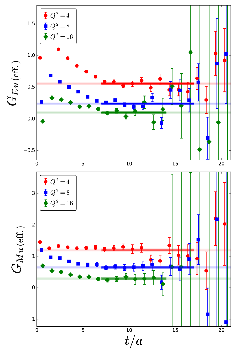
Figure 1: Effective electric and magnetic form factors of the $u$ quark in the nucleon for different values of $Q^{2}$. Results shown are for a single value of $\lambda\neq 0$ (since we are in the linear region, results at different $\lambda$ are statistically identical).

Here we identify that quite clean plateaux are realised up to quite large momentum transfer. As a check on the selected fit window, we ensure that the free-field correlators are sufficiently saturating to the ground-state energy dispersion.

Fig. 2 shows results for the proton electric and magnetic form factors — neglecting disconnected contributions, which are anticipated to be very small at large $Q^{2}$ Green et al. (2015). In the low-$Q^{2}$ region we compare with results computed on the same ensembles using a variationally-improved 3-point function approach, as described in Dragos et al. (2016). Very good agreement is observed in the region of overlap. The statistical signal for the new Feynman–Hellmann approach is seen to extend to much larger $Q^{2}$ than has been accessible in the past.

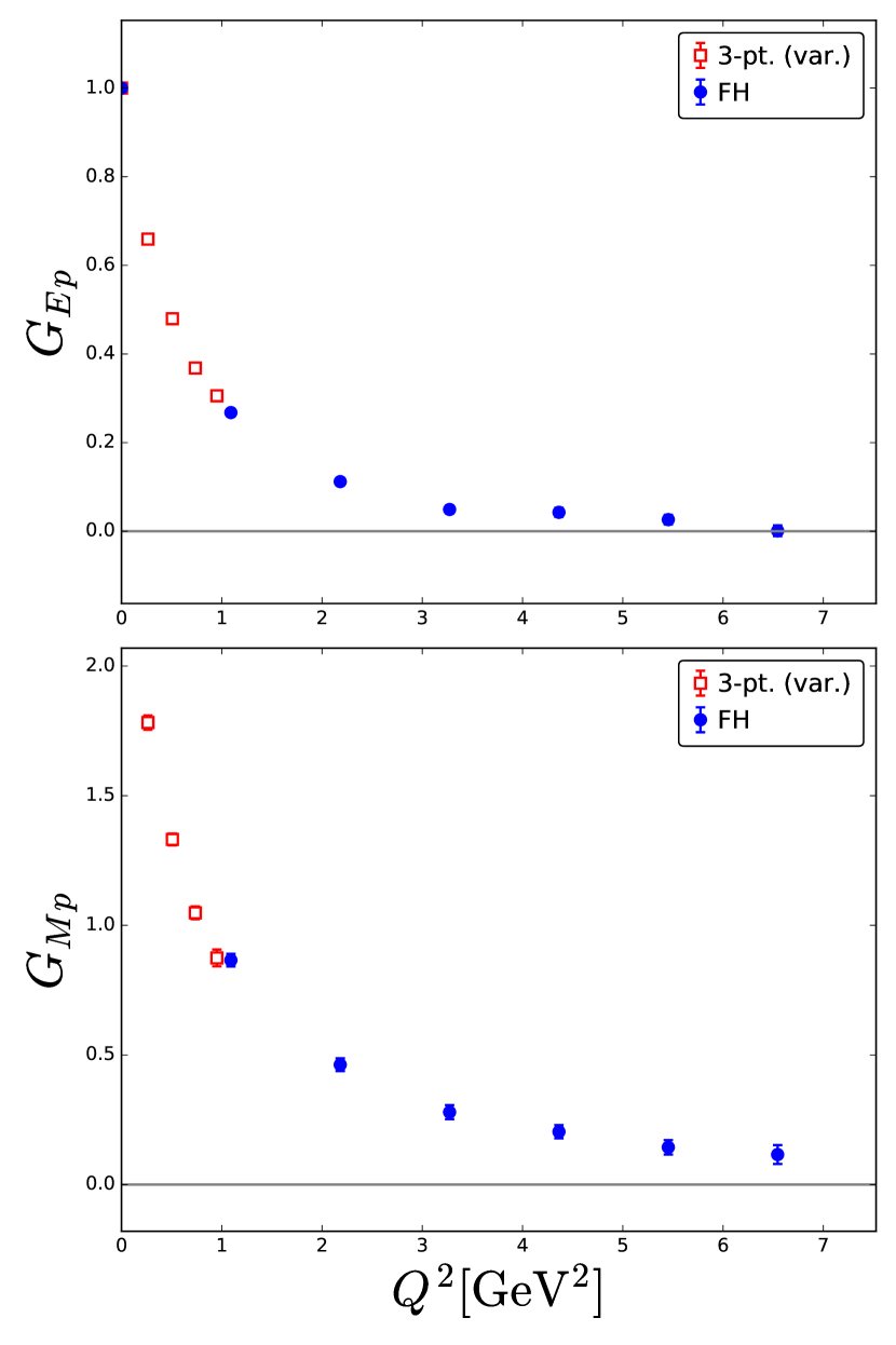
Figure 2: $G_{E}$ and $G_{M}$ for the proton from the Feynman–Hellmann method and a variational method described in Dragos et al. (2016) employed on the same ensemble.

Phenomenologically, the $Q^{2}$-range we are now able to access would allow for tighter constraints to be placed on the distribution of charge and magnetisation in the nucleon at small impact parameter Venkat et al. (2011).

Fig. 3 displays the extraction of the ratio $G_{E}/G_{M}$ as a function of $Q^{2}$, and a comparison to experiment Punjabi et al. (2005); Puckett et al. (2010, 2012). While nothing definitive can be concluded about a potential zero crossing, the overall trend is seen to compare very well with the experimental data.

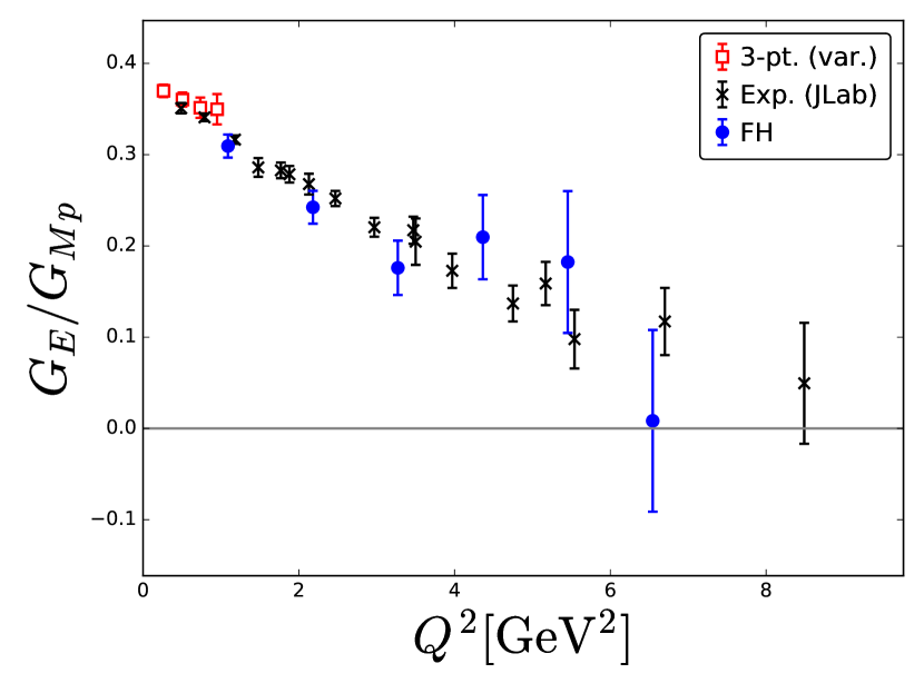
Figure 3: Ratio $G_{E}/G_{M}$ for the proton from application of the Feynman–Hellmann method, from a variational analysis of three-point functions Dragos et al. (2016), and from experiment Punjabi et al. (2005); Puckett et al. (2010, 2012). Note this is not scaled by the magnetic moment of the proton $\mu_{p}$, as this would require phenomenological fits to the low $Q^{2}$ data, which is not the focus of this work.

IV.2 Electromagnetic Form Factor of the Pion

Following a similar analysis as that for the nucleon, we show the determination of the pion form factor and comparison to experiment Huber et al. (2008) in Fig. 4.

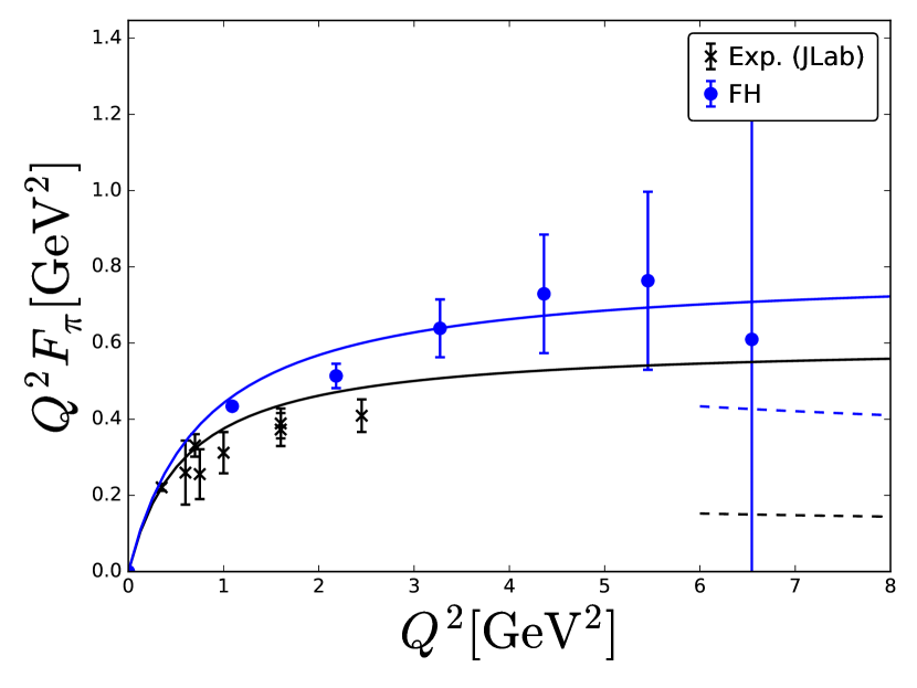
Figure 4: Scaled pion form factor $Q^{2}F_{\pi}$ from the Feynman–Hellmann technique and from experiment Huber et al. (2008). The solid lines are the vector meson dominance at the relevant pion masses, and the dotted lines are the asymptotic values predicted by perturbative QCD (see Chang et al. (2013) for a discussion of this value and its limitations).

The realised statistical signal gives confidence that future lattice simulations will be able to provide important insight into this transition between the perturbative and nonperturbative.

V Conclusion

In this work we have extended the Feynman–Hellmann technique to access non-forward matrix elements. We demonstrate that this provides for a dramatic improvement in the ability to extract nucleon and pion form factors at much higher momentum transfers than previously possible. Before making rigorous comparisons with phenomenology, standard lattice systematics must be further quantified, including quark mass dependence, discretisation artifacts and continuum extrapolation. There is also further potential for increased precision by using improved operators that have better access to high-momentum states, as proposed in Bali et al. (2016).

The high-momentum form factors extracted in this work demonstrate a significantly expanded scope for lattice QCD to address this phenomenologically interesting domain of hadron structure.