Optimizing Cost-Sensitive SVM for Imbalanced Data :Connecting Cluster to Classification

Abstract

Class imbalance is one of the challenging problems for machine learning in many real-world applications, such as coal and gas burst accident monitoring: the burst premonition data is extreme smaller than the normal data, however, which is the highlight we truly focus on. Cost-sensitive adjustment approach is a typical algorithm-level method resisting the data set imbalance. For SVMs classifier, which is modified to incorporate varying penalty parameter(C) for each of considered groups of examples. However, the C value is determined empirically, or is calculated according to the evaluation metric, which need to be computed iteratively and time consuming. This paper presents a novel cost-sensitive SVM method whose penalty parameter C optimized on the basis of cluster probability density function(PDF) and the cluster PDF is estimated only according to similarity matrix and some predefined hyper-parameters. Experimental results on various standard benchmark data sets and real-world data with different ratios of imbalance show that the proposed method is effective in comparison with commonly used cost-sensitive techniques.

1 Introduction

Support vector machines (SVMs) is a popular machine learning technique, owning to its theoretical and practical advantages, which has been successfully employed in many real-world application domains. However, when shifting to imbalanced dataset, SVM will produce an undesirable model that is biased toward the majority class and has low performance on the minority class. Imbalanced learning not only presents significant new challenges to the data research community [1, 2, 3] but also raises many critical questions in real-world data intensive applications.In fact, in most imbalanced learning problems, the misclassification error of the minority class is far costlier than that of the majority class. Following we will give an example to clarify this problem.

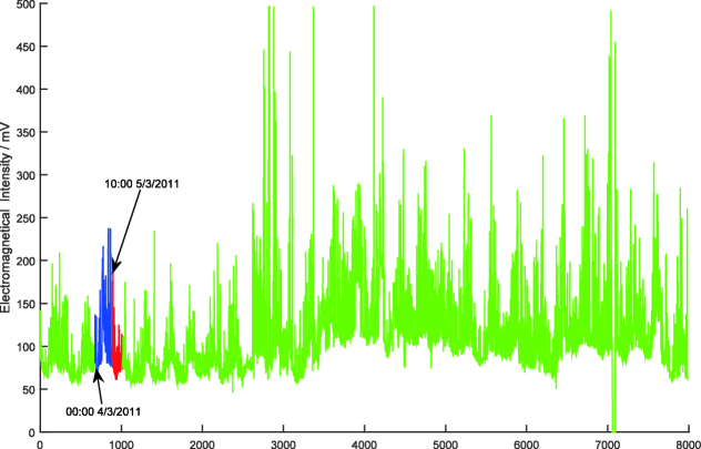
Figure 1: Mine and Gas Burst Electromagnetic Monitoring Data (electromagnetic intensity).The red line means taking place mine and gas burst accident on the date of 05/03/2011. The blue line means the burst premonition data.Compared to normal data,premonition data is extreme small, but which is the object we really focused on.

Figure 1 is the mine and gas burst electromagnetic monitoring data for one month. The red line means taking place mine and gas burst accident on the date of 05/03/2011. One day before the accident, the blue line, means the burst premonition data, which is the object we focused on. If we can classify correctly the premonition data from the other normal data, we can pre-alarm the burst accident and avoid the accident taking place. From the Fig. 1, one month electromagnetic monitoring data is 7989, and there are only 210 premonition data. If we set the premonition data is positive class, and the other normal data is negative class, then the Imbalance Ratio, equals to the ratio of negative class data number and positive class data number, that is 37.04. In fact, the mine and gas burst accident rarely take place, so the imbalance ratio even larger. For this burst electromagnetic monitoring data, we expect positive class and negative class can be classified correctly under this extreme imbalance ratio.

SVMs classifier resist the data imbalance from three categories: Data level, Algorithm level and Hybrid methods. Data-level methods mainly includes oversampling and undersampling, which may have the danger of hardly maintain the original minor data distribution and also may lose the important majority data information seperately. Algorithm-level methods concentrate on modifying existing learners to alleviate their bias towards majority groups. Cost-sensitive methods is a typical representation of this category. The main problem is it is difficult to set the actual values in the cost matrix and often they are not given by expert beforehand in many real-life problems. The penalty parameter(C) is determined empirically, or is calculated according to the evaluation metric, which need to be computed iteratively and time consuming. Decision threshold adjustment is another kind of algorithm-level solution for dealing with class imbalance. Unlike the other correction techniques, decision threshold adjustment strategy runs after modeling a classifier. However, the existing decision threshold adjusting approaches generally give the moving distance of classification boundary empirically, but which cannot answer the question that how far the classification hyperplane should be moved towards the majority class. Hybrid methods usually combine the algorithm-level methods and data-level methods to extract their strong points and reduce their weakness, which can be applied to arbitrary classifier and not only restrict to SVMs.

From the other side, recently, one interesting directions indicates that imbalance ratio is not the sole source of learning difficulties. Even if the disproportion is high, but both classes are well represented and come from non-overlapping distribution we may obtain good classification rates using canonical classifiers. Nevertheless, a good imbalance learning algorithm should fully understand and exploit the minority class structure.

The cluster probability density function(PDF) can naturedly express the class structure and distribution.In this paper, we proposed an cluster Probability optimized CS-SVM method ,named as PCS-SVM ,whose C value determined by the cluster probabilistic density function.We adjust the hyperplane through optimization the value of C for the positive class data, that is adjustment the upper bound of $\alpha$. First, we introduce the L2 norm to optimization function, the dual Lagrangian form of the modified objective function includes the parameter of $C^{+}$ and $C^{-}$. Compared to the traditional SMO algorithm results, the new $\alpha$ expression function is only different from the similarity expression of support vector $x$ and $y$. Then, we construct the connection between similarity and the cluster probability of two points. This is an important measure differentiate the probability density of majority class and minority class. Last, selection two opposite support vector, one is positive but false classified to negative, the other is true negative. By correcting a false negative support vector to a true positive support vector according to cluster possibility, achieve the decision boundary removing toward the majority (negative) class.

2 Related works

In previous work, the class imbalance correction strategies for SVM mainly includes resampling [4] ,cost-sensitive [5, 6], decision threshold adjustment [7], and hybrid methods [8]. Resampling can be accomplished either by oversampling the minority class or undersampling the majority class. However, both sampling techniques have their advantages and disadvantage. Oversampling makes the classifier overfitting and increases the time of modeling, while undersampling often causes information loss.In order to bypass this problem, [4] proposed a Model-Based Oversampling method for imbalanced time series data considering the sequence structure when oversampling. Considering data structure and distribution is the trend of this area.

The Different Error Costs (DEC) method is a cost-sensitive learning solution proposed in [9] to overcome the same cost (i.e. C) for both positive and negative misclassification in the penalty term. As given in Equation (1)

$$\min(\frac{1}{2}\left\|w\right\|^{2}+C^{+}\sum\limits_{y_{i}=+1}{\xi_{i}}+C^{-}\sum\limits_{y_{i}=-1}{\xi_{i}})$$ (1)

$$s.t.\begin{cases}y_{i}-(w^{T}x_{i}+b)\geqslant 1-\xi_{i}\\ \xi_{i}\geqslant 0\\ \end{cases}$$

In this method, the SVM soft margin objective function is modified to assign two misclassification costs, $C^{+}$ and $C^{-}$ is the misclassification cost for positive and negative class examples separately. As a rule of thumb, [10] have reported that reasonably good classification results could be retained from the DEC method by setting the ${C^{-}}/{C^{+}}$ equal to the minority-to-majority class ratio. One-class Learning [11] trained an SVM model only with the minority class examples.  [12] assigned $C^{-}=0$ and $C^{+}=1/{N^{+}}$, these methods have been observed to be more effective than general data rebalancing methods. zSVM is another algorithm modification proposed for SVMs in [13] to learn from imbalance datasets, which is an typical decision threshold adjustment method. In this method, first an SVM model is developed by using the original imbalanced training dataset. Then, the decision boundary of the resulted model is modified to remove its bias toward the majority class. In zSVM method, the magnitude of the $\alpha_{i}^{+}$ is increased by multiplying all of them by a particular value $z$. Then, the modified SVM decision function can be represented as follows:

$$f(x)={\rm sign}(z\ast\sum\limits_{i=1}^{N_{1}}{\alpha_{i}^{+}y_{i}K(x_{i},x)+\sum\limits_{i=1}^{N_{2}}{\alpha_{i}^{-}y_{i}K(x_{i},x)+}b)}$$ (2)

The $z$ value is optimized by gradually increasing the value of $z$ from 0 to some positive value, $M$, and G-mean is adopted as the evaluation measure to determine the optimal $z$. The speed and efficiency of zSVM determined by the step length from 0 to $M$.

3 Proposed method

According to DEC method, the optimized objective function has two loss terms:

$$\min(\frac{1}{2}\left\|w\right\|^{2}+C^{+}\sum\limits_{y_{i}=+1}{\xi_{i}}+C^{-}\sum\limits_{y_{i}=-1}{\xi_{i}})$$ (3)

$$s.t.\begin{cases}y_{i}-(w^{T}x_{i}+b)\geqslant 1-\xi_{i}\\ \xi_{i}\geqslant 0\\ \end{cases}$$

If introduce L2 norm regularization item of slack factor, Equation (3) can be converted into the Equation (4):

$$\frac{1}{2}\left\|w\right\|^{2}+C^{+}\sum\limits_{y_{i}=+1}{\xi_{i}^{2}}+C^{-}\sum\limits_{y_{i}=-1}{\xi_{i}^{2}}$$ (4)

$$s.t.\begin{cases}y_{i}-(w^{T}x_{i}+b)\geqslant 1-\xi_{i}\\ \xi_{i}\geqslant 0\\ \end{cases}$$

The dual Lagrangian form of the modified objective function is:

$$L_{p} =\sum\limits_{i=1}^{p}{\alpha_{i}}-\frac{\left\|w\right\|^{2}}{2}+C^{+}\sum\limits_{\{i|y_{i}=+1\}}^{p}{\xi_{i}^{2}}+C^{-}\sum\limits_{\{i|y_{i}=-1\}}^{p}{\xi_{i}^{2}}$$

$$\quad~{}-\sum\limits_{i=1}^{p}{\alpha_{i}}[y_{i}(w\cdot x_{i}+b)-1+\xi_{i}]-\sum\limits_{i=1}^{p}{\mu_{i}\xi_{i}}$$ (5)

Where $\alpha_{i}\geqslant 0$, and $\mu_{i}\geqslant 0$. Partial deviation formula (5):

$$\frac{\partial L}{\partial w}=\left\|w\right\|-\sum\limits_{i=1}^{p}{\alpha_{i}y_{i}x_{i}}=0\Rightarrow\left\|w\right\|=\sum\limits_{i=1}^{p}{\alpha_{i}y_{i}x_{i}}$$ (6)

$$\frac{\partial L}{\partial b}=\sum\limits_{i=1}^{p}{\alpha_{i}y_{i}}=0$$ (7)

$$\frac{\partial L}{\partial\xi_{i}}=C_{i}^{+}\sum\limits_{y_{i}=+1}{\xi_{i}}+C_{i}^{-}\sum\limits_{y_{i}=-1}{\xi_{i}}-\sum\limits_{i=1}^{p}{\alpha_{i}}-\sum\limits_{i=1}^{p}{\mu_{i}=0}$$ (8)

Substituting (6)–(8) into (5) yields the following:

$$L_{p} =\sum\limits_{i=1}^{p}{\alpha_{i}}-\frac{\left\|w\right\|^{2}}{2}+C^{+}\sum\limits_{\{i|y_{i}=+1\}}^{p}{\xi_{i}^{2}}+C^{-}\sum\limits_{\{i|y_{i}=-1\}}^{p}{\xi_{i}^{2}}$$

$$\quad~{}-\sum\limits_{i=1}^{p}{\alpha_{i}}[y_{i}(w\cdot x_{i}+b)-1+\xi_{i}]-\sum\limits_{i=1}^{p}{\mu_{i}\xi_{i}}$$

$$=\sum\limits_{i=1}^{p}{\alpha_{i}}-\frac{1}{2}\sum\limits_{i=1}^{p}{\alpha_{i}\alpha_{j}y_{i}y_{j}x_{i}^{T}x_{j}}+C^{+}\sum\limits_{\{i|y_{i}=+1\}}^{p}{\xi_{i}^{2}}+C^{-}\sum\limits_{\{i|y_{i}=-1\}}^{p}{\xi_{i}^{2}}-\sum\limits_{i=1}^{p}{(\alpha_{i}+\mu_{i})\xi_{i}}$$ (9)

According to KKT condition, $\sum\limits_{i=1}^{p}{\mu_{i}\xi_{i}}=0$, for $\xi_{i}\neq 0$, so $\mu_{i}=0$. Based on Equation (9), we can get

$$\sum\limits_{i=1}^{p}{\alpha_{i}}=2C^{+}\sum\limits_{y_{i}=+1}^{p}{\xi_{i}}+2C^{-}\sum\limits_{y_{i}=-1}^{p}{\xi_{i}}$$ (10)

Substituting (10) into (9) yields the following

$$L_{p} =\sum\limits_{i=1}^{p}{\alpha_{i}}-\frac{1}{2}\sum\limits_{i=1}^{p}{\alpha_{i}\alpha_{j}y_{i}y_{j}x_{i}^{T}x_{j}}-C^{+}\sum\limits_{\{i|y_{i}=+1\}}^{p}{\xi_{i}^{2}}-C^{-}\sum\limits_{\{i|y_{i}=+1\}}^{p}{\xi_{i}^{2}}$$

$$=\sum\limits_{i=1}^{p}{\alpha_{i}}-\frac{1}{2}\sum\limits_{i=1}^{p}{\alpha_{i}\alpha_{j}y_{i}y_{j}x_{i}^{T}x_{j}}-\frac{\sum\limits_{\{i|y_{i}=+1\}}^{p}{\alpha_{i}^{2}}}{4C^{+}}-\frac{\sum\limits_{\{i|y_{i}=-1\}}^{p}{\alpha_{i}^{2}}}{4C^{-}}$$ (11)

According to SMO algorithm, the original object function including L1 norm regularization item of slack factor for Equation (3) can be described as:

$$\alpha_{2}^{new} =\frac{y_{2}[y_{2}-y_{1}+y_{1}\gamma(K_{11}-K_{12})+v_{1}-v_{2}]}{K_{11}+K_{22}-2K_{12}}$$

$$=\alpha_{2}^{old}+\frac{y_{2}(E_{1}-E_{2})}{K},$$ (12)

Where $E_{i}=f(x_{i})-y_{i},K=K_{11}+K_{22}-2K_{12}$. $K_{ij}=\sum\limits_{i=1}^{p}{x_{i}^{T}x_{j}},f(x_{i})=\sum\limits_{i=1}^{p}{\alpha_{i}y_{i}K_{ij}}+b,v_{i}=f(x_{i})-\sum\limits_{j=1}^{2}{\alpha_{j}y_{j}K_{ij}-b}.$ When $L_{p}=\sum\limits_{i=1}^{p}{\alpha_{i}}-\frac{1}{2}\sum\limits_{i=1}^{p}{\alpha_{i}\alpha_{j}y_{i}y_{j}x_{i}^{T}x_{j}}-\frac{\sum\limits_{\{i|y_{i}=+1\}}^{p}{\alpha_{i}^{2}}}{4C^{+}}-\frac{\sum\limits_{\{i|y_{i}=-1\}}^{p}{\alpha_{i}^{2}}}{4C^{-}}$, we select two opposite symbol support vector to modify $L_{p}$ expression: One is false negative support vector, the other is true positive support vector. Under this condition, given $\alpha_{1}$ is negative and $\alpha_{2}$ is positive, the optimization function turns into:

$$L(\alpha_{2}) =\gamma-s\alpha_{2}+\alpha_{2}-\frac{1}{2}(\gamma-s\alpha_{2})^{2}K_{11}-\frac{1}{2}\alpha_{2}^{2}K_{22}-s(\gamma-s\alpha_{2})\alpha_{2}K_{12}$$

$$\quad~{}-y_{1}(\gamma-s\alpha_{2})v_{1}-y_{2}\alpha_{2}v_{2}+constant-\frac{\alpha_{1}^{2}}{4C^{-}}-\frac{\alpha_{2}^{2}}{4C^{+}}$$ (13)

Then in order to simplicity, we give $C^{-}=1$, and due to $\alpha_{1}=\gamma-s\alpha_{2}$, $s=y_{1}\ast y_{2}=-1$, derivate of Equation (13), the results is

$$-s+1+s\gamma K_{11}-K_{11}\alpha_{2}-\alpha_{2}K_{22}-s\gamma K_{12}+2\alpha_{2}K_{12}+sy_{1}v_{1}-y_{2}v_{2}-\frac{\alpha_{2}}{2C^{+}}-\frac{\alpha_{2}}{2}=0$$

$$\Rightarrow\alpha_{2}^{new}=\frac{y_{2}(E_{1}-E_{2})+\alpha_{2}^{old}(K_{11}+K_{22}-2K_{12})}{K_{11}+K_{22}-2(K_{12}-\dfrac{1}{4C^{+}}-\dfrac{1}{4})}$$ (14)

Compared to Equation (11), the expression of $\alpha_{2}^{new}$ has the change in denominator:

From $$K_{11}+K_{22}-2K_{12} K_{11}+K_{22}-2(K_{12}-\frac{1}{4C^{+}}-\frac{1}{4})$$ to

From the Equation (14), we can conclude that considering the cost of false positive classification can by means of adjusting the value of similarity matrix, that is, update the similarity of $K_{12}$ to $K_{12}^{new}=K_{12}^{old}-\frac{1}{4C^{+}}-\frac{1}{4}$. Through this adjustment, the new value of $\alpha_{2}$ will decrease, under the condition of the other $\alpha$ unchanged, $\left\|w\right\|=\sum\limits_{i=1}^{p}{\alpha_{i}y_{i}x_{i}}$ will also decrease, that is, the max margin of hyperplane will increase. As the positive support vector we selected are unchanged, increasing of max margin means the hyperplane move towards the majority data. Then, we will discuss how to determine the value of $K_{12}^{new}$.

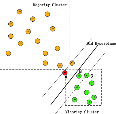
(a) Before adjustment the hyperplane position. False negative support vector A and true positive support vector B belong to different class according to the similarity of A and B

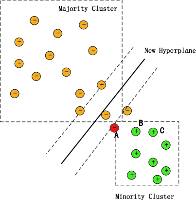
(b) After adjustment the hyperplane position. Adjusting similarity of A and B to the similarity of B and C, the new slack factor C+ is optimized and the new hyperplane is moved toward the majority class

Figure 2: The strategy on how to move the hyperplane toward majority class

In Fig. 2, green points are the minority (positive) class, and the yellow points are the majority (negative) class. At the first, in order to maintain the correctness of majority class, the hyperplane is bias against the minority, whereas the false negative rate is high. Based on the first classifier model, we select two nearest support vectors, one is false negative (point A, in red color), and the other is true positive (point B, in green color). For the old hyperplane (shown as in Fig. 2(a)), point A is more near to the negative point according to the similarity function than the other positive ones. If we can adjust the similarity of point A and its nearest true positive neighbor (such as point B), let the similarity larger than the similarity of point B and its nearest true positive neighbor (such as point C), then the new hyperplane (shown as in Fig. 2(b)) will classify the point A correctly.

The next problem is how to determine the new $K_{12}^{new}$. We only know that using the old learning model, A and B are classified as different class, and B and C are classified as the same class. If we suppose the probabilistic density function of minority cluster is $P_{1}(K_{ij})$, and that of different cluster is $P_{0}(K_{ij})$, then the probability of B and C belong to the minority cluster is $p_{BC}=P_{1}(K_{BC})$, and the probability of A and B belong to the different cluster is $p_{AB}=P_{0}(K_{AB})$, the probability of A and B belong to the minority cluster is $p_{AB}^{new}=P_{1}(K_{AB})$. Then we can get the Equation (15)

$$\frac{K_{AB}}{K_{AB}^{new}}\propto\frac{p_{AB}}{p_{AB}^{new}},~{}~{}\frac{K_{AB}}{K_{BC}}\propto\frac{p_{AB}}{p_{BC}}$$ (15)

Under the same probabilistic density function $P_{1}(K_{ij})$, if we hope $p_{AB}^{new}>p_{BC}$, then $K_{AB}^{new}>K_{BC}$, we can get:

$$\frac{K_{AB}}{K_{AB}^{new}}\leq\frac{K_{AB}}{K_{BC}}\propto\frac{p_{AB}}{p_{BC}}\Rightarrow K_{AB_{new}}\geq k\times K_{AB}\times\frac{p_{BC}}{p_{AB}}$$ (16)

$$K_{AB}^{new}=K_{AB}-\frac{1}{4C^{+}}-\frac{1}{4}>k\times K_{AB}\times\frac{p_{BC}}{p_{AB}}$$

$$\Rightarrow K_{AB}(1-k\times\frac{p_{BC}}{p_{AB}})-\frac{1}{4}>\frac{1}{4C^{+}}$$

$$\Rightarrow K_{AB}\cdot\frac{p_{AB}-k\times p_{BC}}{p_{AB}}-\frac{1}{4}>\frac{1}{4C^{+}}$$

$$\Rightarrow C^{+}>\frac{p_{AB}}{4K_{AB}(p_{AB}-k\times p_{BC})-p_{AB}}$$

Without loss of generality, we set $k=1$. In Equation (16), the value of $C^{+}$ depends on three parameters, $K_{AB},p_{AB}$ and $p_{BC}$. $K_{AB}$ is known, so the problem is how to obtain the $p_{AB}$ and $p_{BC}$. According to the reference  [14], the similarity matrix ${W}$ is modeled as beta distributions, which are defined on the interval of (0, 1), parameterized by two positive shape parameters $\alpha$ and $\beta$. In this case, let $W_{ij}$ is a sample from a beta distribution that is parameterized by $\Theta_{k}=(\alpha_{k},\beta_{k})$, such that it is skewed towards one. If $W_{ij}$ is in off-diagonal blocks, then let $\Theta_{0}=(\alpha_{0},\beta_{0})$ be the parameters for the beta distribution, then it is smaller than any other beta distributions. The probability density function of $W_{ij}$ can be expressed as:

$$p(W_{ij}|\{\Theta_{k}\}_{k=1}^{K},\Theta_{0},Z)=Beta(W_{ij}|\alpha_{0},\beta_{0})^{1-\sum\nolimits_{k}^{K}{z_{ik}z_{jk}}}\prod\limits_{k=1}^{K}{Beta(W_{ij}|\alpha_{k},\beta_{k})^{z_{ik}z_{jk}}}$$ (17)

$z_{n}$ is a K-element cluster indicator $z_{n}=\{z_{nk}\}_{k=1}^{K}$ such that $z_{nk}=1$ if $x_{n}$ belongs to the $k$-th cluster, and otherwise $z_{nk}=0$. $z_{n}$ follows a categorical distribution, and $\pi$ is a sample from a symmetric Dirichlet distribution

The prior distributions to the beta distribution parameters $\Theta_{k}$ and $\Theta_{0}$ are given:

$$p\{\Theta_{k}|\varsigma)\infty Beta(\frac{\alpha_{k}}{\alpha_{k}+\beta_{k}}|\alpha_{\varsigma},\beta_{\varsigma})Lognormal(\alpha_{k}+\beta_{k}|\mu_{\varsigma},\sigma_{\varsigma}^{2})$$ (18)

$$p\{\Theta_{0}|\eta)\infty Beta(\frac{\alpha_{k}}{\alpha_{k}+\beta_{k}}|\alpha_{\eta},\beta_{\eta})Lognormal(\alpha_{\eta}+\beta_{\eta}|\mu_{\eta},\sigma_{\eta}^{2})$$ (19)

We want to calculate the posterior distribution for the latent variables given the observed similarity matrix and the hyper-parameters, i.e.

$$p(\pi,Z,\{\Theta_{k}\}_{k=1}^{K},\Theta_{0}|W,\varsigma,\eta,\lambda)$$ (20)

It is computationally intractable to directly calculate this posterior distribution. Therefore, a vibrational distribution $q(\pi,Z,\{\Theta_{k}\}_{k=1}^{K},\Theta_{0})$ is used to approximate the posterior distribution $p$. This distribution $q$ can be factorized such that

$$q({\pi},Z,\{\Theta_{k}\}_{k=1}^{K},\Theta_{0})=q_{{\pi}}({\pi)}\prod\limits_{n=1}^{N}{q_{z_{n}}(z_{n})}\prod\limits_{k=1}^{K}{q_{\Theta_{k}}(\Theta_{k})}q_{\Theta_{0}}(\Theta_{0})$$ (21)

Then estimate each factorization using $W,\varsigma,\eta,\lambda$ and lastly get the probability of (19).

Lastly, according to the similarity matrix and given hyper-parameters, we can get the element probability density function of $W_{ij}$, namely, the value of $p_{0}$ and $p_{2}$.

4 Complexity analysis

PCS-SVM method includes three steps: first, developing the first SVM model through training original data set; then, computing the new $C$ value; last, using the optimization $C$ value trains the SVM again. The SVM complexity is $O(dn^{2})$, $d$ is the features dimension and $n$ is the data set size. Calculation the posterior distribution for the latent variables given the observed similarity matrix and the hyper-parameters has the complexity of $O(n)$. Whereas, the complexity of our proposed method is $O(dn^{2})$.

5 Experiments

5.1 Data sets and compared methods

We tested the proposed algorithm on 16 Keel data sets and our coal and gas burst monitoring data in first example. We focus on binary-class imbalanced problem, however, our method can be easily extended to multi-class imbalance classification. Information about standard benchmark datasets data sets is summarized in Table 1.

Table 1: Data sets used in this article

Dataset	Imbalance Ratio	Number of instances	Number of attributes
glass1	1.82	214	9
pima	1.87	768	8
wisconsion	1.86	683	9
haber	2.78	306	3
vehicle0	3.25	846	18
yeast3	8.1	1484	8
ecoli3	8.6	336	7
ecolli$-$2-3-5	9.17	244	7
vowel0	9.98	988	13
ecoli$-$0-1_vs_5	11	240	6
yeast$-$1_vs_7	14.3	459	7
abalone9-18	16.4	731	8
flare-F	23.79	1066	11
yeast4	28.1	1484	8
yeast5	32.73	1484	8
abalone19	129.44	4174	8

First, we tested our proposed algorithm in comparison with five other single classification algorithms based on SVM, including:

1. Standard SVM (SSVM): SVM classifier without any class imbalance correction technologies.

2. SVM with random undersampling (SVM-RUS): It firstly adopts RUS to preprocess the original training set, then trains SVM classifier using the balanced training data.

3. SVM with random oversampling (SVM-ROS): It first adopts ROS to preprocess the original training set, then trains SVM with classifier using the balanced training data.

4. SVM with SMOTE (SVM-SMOTE) [15]: It firstly adopts SMOTE algorithm to oversampling the minority class instances and to make the data set balance, then trains SVM classifier using the balanced training data.

5. Weighted SVM (CS-SVM) [10] : It assigns different values for the penalty factor C belong to different classes, to guarantee the fairness of classifier modeling, we make C⁺/C^- equal to imbalance ratio (IR).

In the experiments, for each data set, we performed a fivefold cross validation. In views of the randomness of classification results, we repeated the cross-validation process for 20 times and provided the results in the mean values. All algorithms were implemented in Matlab 2015b running environment and SVM was realized by libSVM toolbox. Specifically, for SVM, polynomial kernel and RBF kernel function was adopted, the penalty factor C and the width parameter $\sigma$ of RBF function were all tuned by using grid search. We evaluated these six classification algorithms by three mainly used evaluation criterions in imbalanced classification: F-measure, G_mean and AUC. For each evaluation criterions and kernel function, we separate our method into two groups: one group is algorithm-level SVM method, our method PCS-SVM is compared with SVM and CS-SVM; The other group is sampling-level SVM method, our method combined with SMOTE named as PCS-SMOTE-SVM is compared with under-sampling(SVM-RUS), oversampling (SVM-ROS) and SMOTE sampling SVM methods (SVM-SMOTE).

5.2 Standard benchmark datasets experiment results

In Table 2 to Table 7, seven SVM methods are evaluated on three measures on sixteen standard benchmark datasets, and each evaluation measure is separated into two groups according to two kernel function: Polynomial kernel (Tables 2, 4, and 6) and RBF kernel (Tables 3, 5, and 7). In the last row of each table, we list the number of winning method for all sixteen datasets. In terms of wins number, in general, PCS-SVM and PCS-SMOTE-SVM method wins more data sets with polynomial kernel than RBF kernel. In algorithm-level SVM methods, PCS-SVM has the clear superiority on F-measure and G-means and on the AUS measure. In sampling-level SVM methods, PCS-SMOTE-SVM outperforms on most of the datasets. The SVM-SMOTE is close to PCS-SMOTE-SVM on three measures with RBF kernel.

Table 2: F-measure values of seven compared single classifiers on 16 Keel data sets, where bold indicates the best result on each data set. (Polynomial kernel function)

F-measure	SVM	CS-SVM	PCS-SVM	SVM-RUS	SVM-ROS	SVM-SMOTE	PCS-SMOTE-SVM
glass1	0.5702	0.5993	0.6226	0.7597	0.7283	0.7649	0.7709
pima	0.3818	0.4277	0.4233	0.5647	0.5176	0.4382	0.4792
wisconsion	0.9062	0.9003	0.9212	0.9657	0.9634	0.9605	0.9665
haber	0.3502	0.3840	0.4437	0.5319	0.5864	0.6367	0.9453
vehicle0	0.9812	0.9847	0.9443	0.9509	0.9863	0.9433	0.9879
yeast3	0.7555	0.7025	0.7462	0.9077	0.9395	0.9586	0.9541
ecoli3	0.5810	0.5618	0.5937	0.7661	0.9394	0.9547	0.9774
ecolli$-$2-3-5	0.6294	0.6305	0.5879	0.6807	0.9710	0.9495	0.9836
vowel0	0.9848	0.9841	0.9765	0.9636	0.9875	0.9991	0.9988
ecoli$-$0-1_vs_5	0.7591	0.7749	0.7940	0.8581	0.9882	0.9905	0.9953
yeast$-$1_vs_7	0.3742	0.2333	0.2270	0.5864	0.8655	0.8662	0.8511
abalone9-18	0.4169	0.4023	0.4608	0.8255	0.8664	0.8528	0.8101
flare-F	0.1213	0.2391	0.2390	0.7199	0.8180	0.8954	0.9589
yeast4	0.2422	0.2957	0.3709	0.6783	0.9036	0.9272	0.9094
yeast5	0.6009	0.6363	0.6392	0.8882	0.9850	0.9851	0.9864
abalone19	0.0236	0.0390	0.0540	0.7644	0.7963	0.8351	0.7430
wins	2/16	3/16	11/16	1/16	2/16	5/16	9/16

Table 3: F-measure values of seven compared single classifiers on 16 Keel data sets, where bold indicates the best result on each data set. (RBF kernel function)

F-measure	SVM	CS-SVM	PCS-SVM	SVM-RUS	SVM-ROS	SVM-SMOTE	PCS-SMOTE-SVM
glass1	0.4678	0.5662	0.6721	0.8351	0.8571	0.8463	0.8416
pima	0.5032	0.4897	0.6274	0.7568	0.7555	0.7717	0.7570
wisconsion	0.9495	0.9501	0.9484	0.9762	0.9686	0.9682	0.9684
haber	0.1458	0.3953	0.4187	0.5860	0.7206	0.7092	0.9195
vehicle0	0.9386	0.9250	0.9253	0.7261	0.9395	0.9226	0.9272
yeast3	0.7698	0.7000	0.7606	0.9124	0.9435	0.9620	0.9580
ecoli3	0.6337	0.6225	0.6658	0.8404	0.8344	0.9551	0.9512
ecolli$-$2-3-5	0.7452	0.7562	0.6000	0.7544	0.9735	0.7792	0.9412
vowel0	0.9772	0.9853	0.9939	0.9691	0.8794	0.9882	0.9994
ecoli$-$0-1_vs_5	0.7383	0.7589	0.7792	0.7581	0.9924	0.7453	0.6749
yeast$-$1_vs_7	0.4712	0.2632	0.2596	0.6518	0.8653	0.8606	0.8670
abalone9-18	0.2487	0.4802	0.5125	0.6699	0.9529	0.9092	0.8864
flare-F	0.2134	0.2726	0.2895	0.7822	0.8819	0.9291	0.9340
yeast4	0.3021	0.3323	0.4201	0.7886	0.8043	0.9373	0.9138
yeast5	0.6821	0.6855	0.7176	0.8580	0.9900	0.9904	0.9892
abalone19	0.0220	0.0223	0.1027	0.4563	0.7404	0.0229	0.7405
wins	4/16	2/16	10/16	1/16	5/16	4/16	6/16

Table 4: G-mean values of seven compared single classifiers on 16 Keel data sets, where bold indicates the best result on each data set. (Polynomial kernel function)

G-mean	SVM	CS-SVM	PCS-SVM	SVM-RUS	SVM-ROS	SVM-SMOTE	PCS-SMOTE-SVM
glass1	0.6597	0.6592	0.6660	0.7711	0.7157	0.7509	0.7626
pima	0.4213	0.4905	0.4931	0.4113	0.5067	0.5105	0.5241
wisconsion	0.9230	0.9150	0.9374	0.9693	0.9623	0.9604	0.9629
haber	0.5072	0.5209	0.6859	0.5328	0.5721	0.6293	0.9669
vehicle0	0.9682	0.9616	0.9633	0.9500	0.9860	0.9644	0.9864
yeast3	0.8495	0.9045	0.8886	0.9048	0.9378	0.9578	0.9515
ecoli3	0.7667	0.7842	0.7999	0.7800	0.9357	0.9524	0.9552
ecolli$-$2-3-5	0.8173	0.8542	0.8468	0.7056	0.9668	0.9465	0.9958
vowel0	0.9932	0.9813	0.9899	0.9619	0.9723	0.9881	0.9988
ecoli$-$0-1_vs_5	0.8755	0.8534	0.8831	0.8794	0.9878	0.9905	0.9954
yeast$-$1_vs_7	0.5334	0.6136	0.7221	0.5878	0.8512	0.8511	0.7989
abalone9-18	0.6681	0.8223	0.8292	0.8214	0.8647	0.8561	0.8480
flare-F	0.4347	0.7108	0.6976	0.7310	0.8166	0.9005	0.9573
yeast4	0.3987	0.7474	0.7498	0.6812	0.9188	0.9257	0.8981
yeast5	0.8042	0.8415	0.8517	0.8883	0.9807	0.9813	0.9865
abalone19	0	0.7190	0.7808	0.7853	0.7820	0.8309	0.7962
wins	2/16	3/16	11/16	2/16	2/16	3/16	9/16

Table 5: G-mean values of seven compared single classifiers on 16 Keel data sets, where bold indicates the best result on each data set. (RBF kernel function)

G-mean	SVM	CS-SVM	PCS-SVM	SVM-RUS	SVM-ROS	SVM-SMOTE	PCS-SMOTE-SVM
glass1	0	0.6610	0.6721	0.8407	0.8569	0.8459	0.8161
pima	0	0.1965	0.6995	0.6183	0.7805	0.7928	0.7806
wisconsion	0.9679	0.9696	0.9683	0.9749	0.9676	0.9673	0.9667
haber	0.2809	0.5614	0.5653	0.6169	0.7159	0.7082	0.9535
vehicle0	0.9574	0.9579	0.9641	0.4984	0.9213	0.9265	0.9298
yeast3	0.8507	0.8921	0.8861	0.9107	0.9420	0.9612	0.9555
ecoli3	0.7714	0.8702	0.8797	0.8483	0.9304	0.9537	0.9698
ecolli$-$2-3-5	0.8454	0	0.8308	0.7800	0.9743	0.8003	0.9844
vowel0	0.9800	0.9950	0.9988	0.9678	0.9788	0.9801	0.9995
ecoli$-$0-1_vs_5	0.8676	0	0.8739	0.8496	0.8925	0.7711	0.7696
yeast$-$1_vs_7	0.5698	0.6452	0.6560	0.6533	0.8565	0.8654	0.8248
abalone9-18	0.3756	0.8301	0.8330	0.6979	0.9105	0.9089	0.8683
flare-F	0	0.8295	0.8068	0.7798	0.8699	0.9346	0.9283
yeast4	0.2019	0.7821	0.7861	0.7834	0.9094	0.9058	0.9132
yeast5	0.8198	0.8463	0.8720	0.8584	0.9728	0.9905	0.9893
abalone19	0	0.6000	0.3720	0.2169	0.6275	0.6477	0.5685
wins	1/16	4/16	11/16	1/16	3/16	6/16	6/16

Table 6: AUS values of seven compared single classifiers on 16 Keel data sets, where bold indicates the best result on each data set. (Polynomial kernel function)

AUS	SVM	CS-SVM	PCS-SVM	SVM-RUS	SVM-ROS	SVM-SMOTE	PCS-SMOTE-SVM
glass1	0.2499	0.1956	0.6721	0.1584	0.8089	0.8334	0.8103
pima	0.5678	0.6019	0.6375	0.4779	0.5751	0.6347	0.6600
wisconsion	0.5610	0.5707	0.5465	0.5104	0.9754	0.9756	0.9767
haber	0.5031	0.5354	0.5674	0.5206	0.6186	0.6776	0.9918
vehicle0	0.8257	0.6626	0.6629	0.0182	0.9955	0.9901	0.9959
yeast3	0.0354	0.0384	0.0430	0.0451	0.9789	0.9877	0.9714
ecoli3	0.5061	0.5812	0.4998	0.1505	0.9577	0.9740	1
ecolli$-$2-3-5	0.5101	0.5597	0.5995	0.6344	0.9782	0.9758	1
vowel0	0.6667	0.6664	0.6665	0.7282	0.9555	0.9657	0.9997
ecoli$-$0-1_vs_5	0.5672	0.5663	0.5533	0.5644	0.9966	0.9972	0.8977
yeast$-$1_vs_7	0.2433	0.2810	0.2761	0.3464	0.8999	0.9183	0.8716
abalone9-18	0.4795	0.5902	0.5967	0.5913	0.9480	0.9300	0.9679
flare-F	0.5457	0.5658	0.5416	0.2308	0.8907	0.9632	0.9688
yeast4	0.1167	0.1253	0.1588	0.2396	0.9672	0.9703	0.9745
yeast5	0.5376	0.6399	0.6415	0.6558	0.9903	0.9914	0.9934
abalone19	0.4885	0.4840	0.4785	0.4926	0.8479	0.8904	0.8691
wins	4/16	5/16	7/16	0/16	0/16	5/16	11/16

Table 7: AUS values of seven compared single classifiers on 16 Keel data sets, where bold indicates the best result on each data set. (RBF kernel function)

AUS	SVM	CS-SVM	PCS-SVM	SVM-RUS	SVM-ROS	SVM-SMOTE	PCS-SMOTE-SVM
glass1	0	0.4576	0.6721	0.0941	0.9133	0.9104	0.9111
pima	0	0.6113	0.6132	0.2358	0.8592	0.9289	0.9048
wisconsion	0.0097	0.0108	0.0117	0.0037	0.9907	0.9901	0.9909
haber	0.4374	0.5506	0.5337	0.5349	0.8092	0.7830	0.9916
vehicle0	0.6656	0.7737	0.7856	0.0555	0.9955	0.9927	0.9966
yeast3	0.5253	0.5338	0.5325	0.0380	0.9809	0.9883	0.9889
ecoli3	0.5885	0.4481	0.5497	0.5812	0.9680	0.9791	0.9786
ecolli$-$2-3-5	0.5599	0.6052	0.5880	0.6393	0.7765	0.7989	1
vowel0	0.6667	0.6667	0.6680	0.4121	0.9776	0.9881	1
ecoli$-$0-1_vs_5	0.5698	0.5589	0.5742	0.6764	0.9989	0.7814	1
yeast$-$1_vs_7	0.2549	0.2448	0.2512	0.2593	0.9326	0.9424	0.9201
abalone9-18	0.5711	0.4877	0.4891	0.6485	0.9838	0.9680	0.9618
flare-F	0.6432	0.5243	0.5127	0.7026	0.9494	0.9543	0.9863
yeast4	0.1668	0.1675	0.1775	0.1358	0.9762	0.9768	0.9745
yeast5	0.4325	0.4372	0.4392	0.5554	0.9975	0.9969	0.9967
abalone19	0.4527	0.2917	0.3219	0.3078	0.7807	0.8967	0.8609
wins	5/16	3/16	8/16	0/16	3/16	5/16	8/16

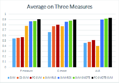
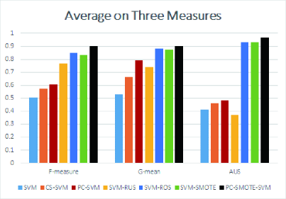
Figure 3: (a) Average on Three Measures (Polynomial kernel function); (b) Average on Three Measures (RBF kernel function)

We compute the average evaluation measure for each SVM method on all datasets, and the results is shown in Fig. 3. The red and black bar represent our proposed method PCS-SVM and PCS-SMOTE-SVM respectively. We can conclude that two kernel function has no obvious influence on average on three measures for all methods. PCS-SVM is the best algorithm in algorithm-level SVM group and for the G-means measure, PCS-SVM even better than SVM-RUS. Four sampling-level algorithms all have the excellent performance in AUS measure and F-measure. PCS-SMOTE-SVM has the best performance in all sixteen date sets and all the average value on three measures are above or very close to 0.9.

5.3 Coal and gas burst monitoring data set experiment results

In this section, we evaluate PCS-SVM and PCS-SMOTE-SVM on our real-world data set: coal and gas burst electromagnetic monitoring data, as shown in Fig. 1. Coal and gas burst is a kind of damaging accident in coal mining. Electromagnetic data can effective reflect the premonition of coal and gas burst accident. So if we can find the premonition of burst accident from the electromagnetic data accurately and timely, we can pre-alarming the burst accident. In our example, the data set is one month electromagnetic monitoring data with the number of 7989, and there are only 210 premonition data, with the imbalance ratio of 37.04. The data set has two features: electromagnetic intensity and electromagnetic pulse. We set the premonition data with positive class and the other normal data is negative class. We expect the premonition data can be classified from the normal data and higher accuracy of these premonition data than normal data. Because negative class is so huge, we random undersampling negative data to 2000 and SMOTE positive data to 500. As is concluded in Section 4.2, SMOTE has the better performance than ROS and RUS method, and PCS-SVM and PCS-SMOTE-SVM method wins more data sets with polynomial kernel than RBF kernel, we only use SMOTE to oversampling data and adopt polynomial kernel. In this experiment, besides three evaluations we have used, the sensitivity and specificity also be evaluated in order to describe the accuracy rate of positive class. The results are shown in Table 8.

Table 8: The evaluate results on electromagnetic monitoring data

	Sensitivity	Specificity	F-measure	G-mean	AUC
SVM	0.0211	0.9722	0.0379	0.1432	0.4094
CS-SVM	0.6599	0.3509	0.2670	0.2146	0.4923
SMOTE-SVM	0.5445	0.4575	0.2820	0.4136	0.4816
PCS-SVM	0.6055	0.3910	0.3104	0.2244	0.4998
PCS-SMOTE-SVM	0.9935	0.1411	0.3713	0.4036	0.7770

From the Table 8, we can easily conclude that both PCS-SVM and PCS-SMOTE-SVM outperform compared method. Especially, sensitivity is higher than specificity which attain our expectation. PCS-SMOTE-SVM has the best performance on all the evaluation measures and the AUC values reaches 0.7770, compared to SMOTE-SVM, improve 29.54%.

6 Conclusion and future work

This paper presents a novel C value optimization method on the basis of cluster probability density function, which is estimated only using similarity matrix and some predefined hyper-parameters. Experimental results on various standard benchmark datasets and real-world data with different ratios of imbalance show that the proposed method is effective in comparison with commonly used cost-sensitive techniques.

For future work, we plan to leverage multi-view feature representations  [16, 17, 18, 19] to improve the performance of SVMs for imbalanced data set.

References

- [1] Yang Wang, Xuemin Lin, Lin Wu, Wenjie Zhang, Qing Zhang, Xiaodi Huang: Robust Subspace Clustering for Multi-View Data by Exploiting Correlation Consensus. IEEE Trans. Image Processing 24(11): 3939-3949 (2015)
- [2] Yang Wang, Xuemin Lin, Qing Zhang, Lin Wu: Shifting Hypergraphs by Probabilistic Voting. PAKDD (2) 2014: 234-246
- [3] Yang Wang, Xuemin Lin, Lin Wu, Wenjie Zhang: Effective Multi-Query Expansions: Collaborative Deep Networks for Robust Landmark Retrieval. IEEE Trans Image Processing 2017. DOI:10.1109/TIP.2017.2655449
- [4] Z. Gong and H. Chen, “Model-Based Oversampling for Imbalanced Sequence Classification,” in Proceedings of the 25th ACM International on Conference on Information and Knowledge Management - CIKM ’16, 2016, pp. 1009–1018.
- [5] F. Cheng, J. Zhang, and C. Wen, “Cost-Sensitive Large margin Distribution Machine for classification of imbalanced data.,” Pattern Recognit. Lett., vol. 80, pp. 107–112, 2016.
- [6] P. Cao, D. Zhao, and O. R. Zaïane, “A PSO-Based Cost-Sensitive Neural Network for Imbalanced Data Classification. BT - Trends and Applications in Knowledge Discovery and Data Mining - PAKDD 2013 International Workshops: DMApps, DANTH, QIMIE, BDM, CDA, CloudSD, Gold Coast, QLD, Australia, A.” pp. 452–463, 2013.
- [7] G. Ristanoski, W. Liu, and J. Bailey, “Discrimination aware classification for imbalanced datasets,” in Proceedings of the 22nd ACM international conference on Conference on information & knowledge management - CIKM ’13, 2013, pp. 1529–1532.
- [8] H. Cao, V. Y. F. Tan, and J. Z. F. Pang, “A Parsimonious Mixture of Gaussian Trees Model for Oversampling in Imbalanced and Multimodal Time-Series Classification.,” IEEE Trans. Neural Netw. Learn. Syst., vol. 25, no. 12, pp. 2226–2239, 2014.
- [9] C. C. and N. C. K. Veropoulos, “Controlling the sensivity of support vector machines,” 1999.
- [10] R. Akbani, S. Kwek, and N. Japkowicz, “Applying Support Vector Machines to Imbalanced Datasets BT - Machine Learning: ECML 2004: 15th European Conference on Machine Learning, Pisa, Italy, September 20-24, 2004. Proceedings,” J.-F. Boulicaut, F. Esposito, F. Giannotti, and D. Pedreschi, Eds. Berlin, Heidelberg: Springer Berlin Heidelberg, 2004, pp. 39–50.
- [11] B. Raskutti and A. Kowalczyk, “Extreme Re-balancing for SVMs: A Case Study,” SIGKDD Explor. Newsl., vol. 6, no. 1, pp. 60–69, 2004.
- [12] A. Kowalczyk and B. Raskutti, “One Class SVM for Yeast Regulation Prediction,” SIGKDD Explor. Newsl., vol. 4, no. 2, pp. 99–100, 2002.
- [13] T. Imam, K. M. Ting, and J. Kamruzzaman, “z-SVM: An SVM for Improved Classification of Imbalanced Data,” in AI 2006: Advances in Artificial Intelligence: 19th Australian Joint Conference on Artificial Intelligence, Hobart, Australia, December 4-8, 2006. Proceedings, A. Sattar and B. Kang, Eds. Berlin, Heidelberg: Springer Berlin Heidelberg, 2006, pp. 264–273.
- [14] J. Chen and J. Dy, A Generative Block-diagonal Model for Clustering, in Proceedings of the Thirty-Second Conference on Uncertainty in Artificial Intelligence, 2016, pp. 112 C121.
- [15] N. V Chawla, K. W. Bowyer, L. O. Hall, and W. P. Kegelmeyer, SMOTE: Synthetic Minority Over-sampling Technique, J. Artif. Int. Res., vol. 16, no. 1, pp. 321 C357, 2002.
- [16] Yang Wang, Xuemin Lin, Lin Wu, Wenjie Zhang: Effective Multi-Query Expansions: Robust Landmark Retrieval. ACM Multimedia 2015: 79-88
- [17] Yang Wang, Xuemin Lin, Lin Wu, Qing Zhang, Wenjie Zhang: Shifting multi-hypergraphs via collaborative probabilistic voting. Knowl. Inf. Syst. 46(3): 515-536 (2016)
- [18] Yang Wang, Wenjie Zhang, Lin Wu, Xuemin Lin, Xiang Zhao: Unsupervised Metric Fusion Over Multiview Data by Graph Random Walk-Based Cross-View Diffusion. IEEE Trans. Neural Netw. Learning Syst. 28(1): 57-70.
- [19] Yang Wang, Wenjie Zhang, Lin Wu, Xuemin Lin, Meng Fang, Shirui Pan. Iterative Views Agreement: An Iterative Low-Rank Based Structured Optimization Method to Multi-View Spectral Clustering. IJCAI 2016: 2153-2159.