Wide-Field ¹²CO ($J=2-1$) and ¹³CO ($J=2-1$) Observations toward the Aquila Rift and Serpens Molecular Cloud Complexes. I. Molecular Clouds and Their Physical Properties

Abstract

We present results of wide-field ¹²CO ($J=2-1$) and ¹³CO ($J=2-1$) observations toward the Aquila Rift and Serpens molecular cloud complexes (25${}^{\circ}<l<33^{\circ}$ and $1^{\circ}<b<6^{\circ}$) at an angular resolution of 3^′.4 ($\approx$ 0.25 pc) and at a velocity resolution of 0.079 km s^-1 with the velocity coverage of $-5$ km s${}^{-1}<V_{\rm LSR}<$ 35 km s^-1. We found that the ¹³CO emission better traces the structures seen in the extinction map and derived the $X_{\rm{}^{13}CO}$-factor of this region. Applying SCIMES to the ¹³CO data cube, we identified 61 clouds and derived their masses, radii, and line widths. The line-width-radius relation of the identified clouds basically follows those of nearby molecular clouds. Majority of the identified clouds are close to virial equilibrium although the dispersion is large. By inspecting the ¹²CO channel maps by eye, we found several arcs which are spatially extended to 0.2 $-$ 3 degree in length. In the longitude-velocity diagrams of ¹²CO, we also found the two spatially-extended components which appear to converge toward Serpens South and W40 region. The existence of two components with different velocities and arcs suggests that large-scale expanding bubbles and/or flows play a role in the formation and evolution of the Serpens South and W40 cloud.

1. Introduction

Large-scale molecular line observations are important to unveil how molecular clouds have been formed and evolved because in interstellar space, large-scale dynamical events such as bubbles and supersonic turbulent flows often influence the structure and kinematics of molecular gas where star formation happens (e.g., Dame & Thaddeus, 1985; Dame et al., 1987). In the present paper, we investigate the cloud structure and kinematics of the Aquila Rift and Serpens molecular cloud complex, on the basis of large-scale multi-CO line observations.

Aquila Rift is located in the first Galactic quadrant, spanning from 20^∘ to 40^∘ in Galactic longitude and $-1^{\circ}$ to 10^∘ in Galactic latitude. It appears in the optical image as a dark lane that divides the bright band of the Milky Way longitudinally (Prato et al., 2008). The total molecular gas mass is estimated to be about a few $\times 10^{5}M_{\odot}$ on the basis of the CO ($J=1-0$) observations with an angular resolution of about 7^′.5 (Dame & Thaddeus, 1985; Dame et al., 1987). Dobashi et al. (2005) identified a number of dark clouds in this region using the Digitized Sky Survey visual extinction data. These previous studies indicate that the region has complex density and velocity structure, suggesting that the dynamical interaction and events might be ongoing and/or have happened in this region (Prato et al., 2008). In fact, Frisch (1998) pointed out that several nearby superbubble shells appear to converge toward the Aquila Rift region. In the southern part of Aquila Rift, Kawamura et al. (1999) suggested that the virial mass of the molecular cloud complex is significantly larger than the molecular gas mass and star formation is less active.

However, the molecular gas distribution and star formation activity in the northern part above the Galactic plane have not been extensively explored so far. Here, we focus on the western part of Aquila Rift, which stretches from $25^{\circ}$ to $33^{\circ}$ in Galactic longitude and $1^{\circ}$ to $6^{\circ}$ in Galactic latitude. The western part of Aquila Rift contains several active star-forming regions such as Serpens Main, Serpens South, W40, and MWC 297. In a well-studied nearby cluster-forming region, Serpens main star-forming region (Eiroa et al., 2008), several young protostars are blowing out of powerful collimated outflows. Recently, the Spitzer observations have discovered an extremely-young embedded cluster of low-mass protostars, Serpens South, which contains a large number of Class 0/I objects (Gutermuth et al., 2008; André et al., 2010; Tanaka et al., 2013; Konyves et al., 2015). In fact, Nakamura et al. (2011) detected a number of CO outflows in the central part of Serpens South (see also Plunkett et al., 2015). In more evolved star-forming region, W40 H ii region, the expanding structure affects the star formation in this region (Shimoikura et al., 2015). Recent studies also suggest that cloud-cloud collision may have triggered star formation in Serpens Main region (Duarte-Cabral et al., 2011) and Serpens South region (Nakamura et al., 2014). MWC 297 is an embedded young massive B1.5Ve star, one of the closest massive stars (Drew et al., 1997). A molecular outflow is detected toward the MWC 297 region, implying that active star formation is ongoing. In spite of the effort of these previous studies, it remains uncertain why star formation in the western part is much more active than the southern part.

In addition, the distance to the Aquila Rift and Serpens cloud complex is somewhat controversial. For the Serpens Main star-forming region, the distance of $\sim$ 260 pc has been used (Eiroa et al., 2008). This distance determination is based mainly on measurements of the extinction suffered by stars in the direction of Serpens. However, recent VLBA measurements of young stellar objects, EC95a and EC95b, suggest a larger distance of 415 pc (Dzib et al., 2010). For the W40 cloud, the distance is estimated to be $300-900$ pc and has not yet been determined to a satisfactory precision (Rodney & Reipurth, 2008). The distance to MWC 297 is estimated to be 250 pc (Drew et al., 1997) or 450 pc (Hillenbrand et al., 1992) on the basis of measurements of the extinction of stars, and the uncertainty is a similar degree to other regions in the Aquila Rift and Serpens cloud complexes. Serpens South has a Local Standard of Rest (LSR) velocity similar to Serpens Main (Gutermuth et al., 2008). This fact suggests that Serpens South may have a distance similar to Serpens Main. However, no accurate distance measurements have been done so far. The uncertainty of the distance makes it difficult to clarify the cloud dynamical states in the Aquila Rift and Serpens cloud complexes. In the present paper, we compare the cloud physical quantities for both 260 pc and 415 pc.

In the present paper, as a first step toward a better understanding of star formation activity in the Aquila Rift and Serpens molecular cloud complexes, we investigate the large-scale molecular cloud structure of the region with an angular resolution of about 3^′, on the basis of wide field ¹²CO ($J=2-1$) and ¹³CO ($J=2-1$) observations. In Section 2, we present the detail of our observations. In Section 3, we describe the large-scale CO structure in this region. We find several arcs that may have been formed by the large-scale flows. We also derive the $X_{\rm CO}$ factor of this region by comparing CO velocity-integrated intensity map and the 2MASS extinction map. In Section 4, we apply SCIMES (Colombo et al., 2015) to the CO data cube, and identify the clouds. In the present paper, we call structures identified by SCIMES as ”clouds”. Then, we attempt to assess their dynamical states. Finally, we briefly summarize the main results in Section 5.

2. Observations and Data

2.1. 1.85-m Observations

We carried out ¹²CO ($J=2-1$), ¹³CO ($J=2-1$), and C¹⁸O ($J=2-1$) mapping observations toward the Aquila Rift and Serpens molecular cloud complexes, during the periods from 2012 February to 2012 March and from 2012 December to 2013 March. The observations were done in the on-the-fly (OTF) mapping mode with a 2SB SIS mixer receiver on the 1.85 m radio telescope of Osaka Prefecture University. The telescope is installed at the Nobeyama Radio Observatory (NRO). The image rejection ratio (IRR) was measured to be 10 dB or higher during the observations. At 230 GHz band, the telescope has a beam size of $2^{\prime}.7$ (HPBW) and a main beam efficiency of $\eta$ = 0.6. At the back end, we used a digital Fourier transform spectrometer (DFS) with 16384 channels that covers the 1 GHz bandwidth, which allows us to obtain the three molecular lines, ¹²CO ($J=2-1$), ¹³CO ($J=2-1$), and C¹⁸O ($J=2-1$), simultaneously. In the present paper, we focus on the ¹²CO ($J=2-1$) and ¹³CO ($J=2-1$) data. The frequency resolution was set to 61 kHz, which corresponds to the velocity resolution of $\sim$ 0.08 km s^-1 at 220 GHz. During the observations, the system noise temperatures were about 200 $-$ 400 K in a single sideband. Further description of the telescope is given by Onishi et al. (2013).

The observed area was a rectangle area with 40 square degrees whose coordinates of the bottom-left-corner (BLC) and top-right-corner (TRC) are $(l,b)\simeq$ ($33^{\circ}$, $1^{\circ}$) and ($25^{\circ}$, $6^{\circ}$), respectively. The area was divided into 40 boxes of $1^{\circ}\times 1^{\circ}$, each of which was scanned a few times in both Galactic longitude and lattitude with a row spacing of $1^{\prime}$ at a scan speed of $1$ sec per row. The standard chopper wheel method was used to correct the output signals for the atmospheric attenuation and to convert them into the antenna temperatures ($T_{A}^{*}$). Then, we corrected the antenna temperatures for the main beam efficiency to obtain the brightness temperatures $T_{\rm mb}$ (= $T_{A}^{*}/\eta$). We applied a convolution technique with a Gaussian function to calculate the intensity onto a regular grid with a spacing of 1^′. The resultant effective angular resolution was $3^{\prime}.4$. The rms noise levels of the final ¹²CO and ¹³CO maps vary from box to box, and are summarized in Appendix A (Tables A1 and A2). The average noise levels are given in the last column of Table 1.

2.2. 2MASS Extinction Data

To compare with the molecular line data, we downloaded the near-infrared (NIR) color excess map of $E(J-H)$ shown in Figure 1(a) from http://darkclouds.u-gakugei.ac.jp/2MASS/download.html. The map was originally generated by Dobashi (2011) and Dobashi et al. (2013) utilizing the 2MASS point source catalog, and sampled at the same $1^{\prime}$ grid along the galactic coordinates as the CO data. The angular resolution, however, varies in the range of $0.8^{\prime}-11^{\prime}$, because the map was drawn using the ”adaptive grid” technique to achieve a constant noise level. See Dobashi (2011) and Dobashi et al. (2013) for details. In Section 3.2, using the $E(J-H)$ color excess map, we construct the visual extinction map of the Aquila Rift and Serpens cloud complexes, which is presented in Figure 1(c). Some of the active star-forming regions are designated in Figure 1(c).

3. Results

3.1. Global Molecular Gas Distribution

Figure 2 shows the ¹²CO ($J=2-1$) velocity integrated intensity map toward the Aquila Rift and Serpens molecular cloud complexes. For comparison, the ¹²CO ($J=2-1$) channel maps and the longitude-velocity diagram averaged over the Galactic latitude range of $1^{\circ}\leq b\leq 6^{\circ}$ are shown in Figures 3 and 4, respectively. ¹²CO, ¹³CO, and C¹⁸O line spectra at several positions are also presented in Figure 5. The CO emission is extended almost over the entire mapped area. The CO integrated intensity takes its maximum at the position of $(l,b)\simeq(31^{\circ}35^{\prime},\ 5^{\circ}20^{\prime})$, which is in the molecular cloud associated with the Serpens cluster A. The ¹²CO emission associated with the Serpens cluster B is not so prominent. Other CO peaks are located at $(l,b)\simeq(28^{\circ}45^{\prime},\ 3^{\circ}32.5^{\prime})$, which corresponds to the W40 H ii region, and at the position of $(l,b)\simeq(29^{\circ}50^{\prime},\ 2^{\circ}13^{\prime})$. Most CO emission comes from the velocity range of 0 $-$ 20 km s^-1, which is presumably associated with the Gould Belt, an expanding ring of stars in the local spiral arm.

A prominent feature of the longitude-velocity and channel maps is the existence of two spatially-extended components with different velocities, $V_{\rm LSR}\sim 5$ km s^-1 and 8 km s^-1 in the part of Galactic longitude smaller than 29^∘. The former component is recognized in the first panel ($V_{\rm LSR}=3$ km s^-1) of the velocity channel map in Figure 3. The latter is more spatially-extended in the entire observed area. In the ¹²CO longitude-velocity diagram (Figure 4), the two components appear to converge at around the position of the Serpens South and W40 cloud, which might suggest the two components interact with each other, triggering the active star formation in Serrpens South and W40. However, there is also a possibility that the two components are simply overlapped along the line-of sight.

Another interesting characteristic is that in the channel maps, some velocity-coherent, large-scale linear structures can be recognized. For example, in both 1$-$4 km s^-1 (the first panel of Figure 3) and 9$-$13 km s^-1 (the third panel of Figure 3) panels, a couple of large arcs with similar morphologies are recognized. To emphasize these structures, we show in Figures 6a and 6b, the ¹²CO intensity maps integrated over the velocity intervals of $4.5-6$ km s^-1 and $6-9$ km s^-1, respectively, where the velocity-coherent linear structures are indicated with dashed curves. Assuming a distance of 260 pc, these linear structures are found to be very large as about 6 $-$ 20 pc in length. Hereafter, we call these linear structures arcs. Since ISM is highly turbulent, such large-scale structures should be created by large-scale dynamical events such as large-scale turbulent flows and/or supernova shocks. These arcs might be created by the superbubbles converging toward the observed area (Frisch, 1998).

For comparison, we show ¹³CO ($J=2-1$) velocity integrated intensity map toward the Aquila Rift and Serpens molecular cloud complexes in Figure 7. The ¹³CO ($J=2-1$) channel maps and the longitude-velocity diagram integrated over the Galactic latitude range of $1^{\circ}\leq b\leq 6^{\circ}$ are indicated in Figures 8 and 9, respectively. Comparison between the ¹³CO map and the extinction map indicates that the ¹³CO emission better traces the extinction image than the ¹²CO emission (Figure 7b). Two components with different velocities seen in the ¹²CO channel maps are also recognized in the ¹³CO channel maps. Some arcs identified with ¹²CO can be seen in the ¹³CO map, indicating that densities of those arcs are relatively high. The longitude-velocity diagram shows that only 8km s^-1 component is prominent in the ¹³CO map.

3.2. Comparison of Molecular Gas and Visual Extinction

Here we compare the CO data with dust detected in the $E(J-H)$ map. While the CO lines are emitted only in dense regions (e.g., $\gtrsim 10^{2-3}$ cm^-3), the color excess map traces the total dust column density along the line of sight including diffuse regions in the background (or foreground) unrelated to the CO emitting volumes. We therefore should remove the background of the $E(J-H)$ map to compare the two dataset directly.

For compact clouds at high latitudes, such removal of the background can be easily done by subtracting a constant or by fitting the background with an exponential function of the Galactic latitudes $b$ (e.g., Dobashi et al., 2005). Those methods, however, do not work well in the case of the clouds in Aquila Rift, because the region suffers from great complexity over a large extent. We therefore decided to use the following procedure to remove the background: We first defined the temporary background as the regions without showing apparent small scale-structures in Figure 1(a), and masked the apparent clouds in the figure by eye-inspection. We then fitted the unmasked pixels by two dimensional (2D) polynomial function of $N=4$ degree, and subtracted it from the original $E(J-H)$ map to convert the residual map to $A_{V}$ as

$$A_{V}=9.35E(J-H)\ ,$$ (1)

where the coefficient is calculated using the reddening law found by Reike & Lebofsky (1985). We smoothed the resulting $A_{V}$ map with $10\times 10$ pixels ($=10^{\prime}\times 10^{\prime}$), and redefined the background as the regions with $A_{V}<0.5$ mag in the smoothed map. The background regions defined in this manner is shown in Figure1 (b). To better assess the background, we further fitted the background regions in the figure with a 2D polynomial function with higher orders ($N$), and decided to adopt $N=8$ degree to produce the final $A_{V}$ map which we use in the following analyses. We show the map in Figure 1(c). The maximum value found in the map is $A_{V}\simeq 50$ mag, and the $1\sigma$ noise level of the map is $\delta A_{V}\simeq 2.5$ mag.

In order to infer the possible systematic error due to the background removal, we reproduced background maps with different orders of polynomials $N=4-9$ to derive $A_{V}$ maps in the same way as described above. We found that the $A_{V}$ values in the resulting maps vary by $\sim 3$ mag at most depending on $N$, which we regard as the uncertainty in our $A_{V}$ map arising from the background determination.

To compare the CO and $A_{V}$ data directly, we smoothed both of the data to the common 6^′ (FWHM) angular resolution. We excluded some positions from the analyses where the $A_{V}$ map suffers from a very low angular resolution ($>6^{\prime}$). Figures 10 and 11 show the relations of the ¹³CO and ¹²CO integrated intensities vs. $A_{V}$, respectively. In the case of the ¹³CO emission, the relation is simple and can be fitted by a linear function, while that of the ¹²CO emission is complex mainly due to the heavy saturation at higher $A_{V}$. This saturation is presumably due to the fact that ¹²CO emission becomes optically thick at higher $A_{V}$.

In order to estimate the total masses of clouds that we identified with the molecular data (see Section 4), we formulate the dependence of $W_{\rm{}^{13}CO}$ on $A_{V}$. For this purpose, we fitted the $W_{\rm{}^{13}CO}$ vs. $A_{V}$ relation by a linear function,

$$W_{\rm{}^{13}CO}={a_{0}}{A_{V}}\ ,$$ (2)

where the coefficient best fitting the relation is

$$a_{0}=0.285\pm 0.001\ {\rm K\ kms^{-1}mag^{-1}}\ .$$ (3)

The relations of $W_{\rm{}^{12}CO}$ vs. $A_{V}$ and $W_{\rm{}^{13}CO}$ vs. $A_{V}$ appear to be better fitted with exponential functions. Here, we attempt to fit these relations with exponential functions. Similar attempt has been done by Pineda et al. (2010).

For the $W_{\rm{}^{13}CO}$ vs. $A_{V}$ relation, we consider the following exponential function,

$$W_{\rm{}^{13}CO}={a_{1}}\left[{1-\exp(-{a_{2}}{A_{V}})}\right]\ ,$$ (4)

where $a_{1}$ and $a_{2}$ are constants.

The coefficients best fitting the relation are obtained as

$$a_{1}=12.16\pm 0.55\ {\rm K\ kms^{-1}},$$ (5)

and

$$a_{2}=0.0269\pm 0.014\ {\rm mag^{-1}}.$$ (6)

For the $W_{\rm{}^{12}CO}$ vs. $A_{V}$ relation, we consider the following exponential function

$$W_{\rm{}^{12}CO}={b_{1}}\left[{1-\exp(-{b_{2}}{A_{V}})}\right],$$ (7)

where $b_{1}$ and $b_{2}$ are constants.

The coefficients best fitting the relation are derived as

$$b_{1} = 16.8\pm 4.4{\rm K\ km\ s^{-1}},$$ (9)

$${\rm and}$$

$$b_{2} = 0.37\pm 0.18\ {\rm mag^{-1}}.$$ (10)

The relations expressed by Equations (4) and (7) are shown in Figures 10 and 11, respectively.

The $X_{\rm CO}$ factor gives a scaling between CO luminosity and molecular cloud mass and we use $X_{\rm CO}$ to derive the masses of the clouds identified in the next section. As shown above, $W_{\rm{}^{13}CO}$ is well correlated with $A_{V}$. Therefore, we use ¹³CO emission to identify the clouds and evaluate their masses. The $X_{\rm{}^{13}CO}$ factor is calculated as

$$X_{\rm{}^{13}CO}\equiv{N_{\rm H_{2}}\over W_{{}^{13}CO}}=3.3\times 10^{21}{\rm cm^{-2}K^{-1}km^{-1}s},$$ (12)

where we used Equation (2) and assumed the relation of $N({\rm H_{2}})/A_{V}=9.4\times 10^{20}$ cm^-2 mag^-1 and $R_{V}=3.1$ (Bohlin et al., 1978).

Adopting the above $X_{\rm{}^{13}CO}$ factor, the total molecular gas mass in the observed region is estimated to be about $1\times 10^{5}M_{\odot}$ under the assumption of $d=260$ pc.

The $X_{\rm CO}$-factors are usually estimated by using the ¹²CO ($J=1-0$) line. For our Galaxy, the averaged $X_{\rm{}^{12}CO}$ is evaluated to be $2\times 10^{20}$ cm^-2 K^-1 km^-1 s with an uncertainty of $\pm 30\%$ (Bolatto et al., 2013). This values vary from region to region. For example, Pineda et al. (2010) derived the $X$-factor of $(1.6\sim 12)\times 10^{20}$ cm^-2 K^-1 km^-1 s in the Taurus molecular cloud. For L1551, Lin et al. (2016) measured the $X_{\rm CO}=1.08\times 10^{20}$ cm^-2 K^-1 km^-1 s.

Here, we attempt to compare our $X$-factor using higher transition with these previous values using the $J=1-0$ line. We choose the Serpens Main Cloud because this region basically has single component. In constrast, the Serpens South+W40 region contains multiple-components. The part including Serpens Main Cloud has $W_{\rm{}^{12}CO}=20-25$ K km s^-1 and $W_{\rm{}^{13}CO}=4-6$ K km s^-1. In the part including Serpens Main Cloud, the mean intensity of ¹²CO $(J=2-1)$ and line width are evaluated to be 5.6 K and 3.5 km s^-1, respectively. The mean intensity of ¹³CO ($J=2-1$) and line width are evaluated to be 2.5 K and 2.5 km s^-1, respectively. Adopting the H₂ density of $10^{3}$ cm^-3, $T=10$ K, the H₂ column density of $1\times 10^{21}$ cm^-2 ($A_{V}\approx 15-20$), the CO fractional abundance of $10^{-4}$, and ¹²CO/¹³CO ratio of 80, the intensity of ¹²CO ($J=1-0$) is derived as $\sim$ 7 K using RADEX (Van der Tak et al., 2007), and thus $W_{\rm 12CO(1-0)}=25$ K km s^-1. Thus, we can convert our $X_{\rm 13CO(2-1)}$ to $X_{\rm 12CO(1-0)}=5.6\times 10^{20}$ cm^-2 K^-1 km^-1 s, which is about 2.5 times larger than the standard value of Bolatto et al. (2013). Therefore, our $X_{\rm 13CO(2-1)}$ value is consistent with the previous estimation, taking into account a large variation of $X$-factor values.

4. Identification of Molecular Clouds

As shown in Section 3, the correlation between ¹³CO integrated intensity and extinction $A_{V}$ is reasonably good. Therefore, we identify molecular clouds from the ¹³CO data cube and derive their physical quantities such as cloud masses, radii, and line widths.

There are several methods proposed to identify clouds. In the following, we apply a new method called SCIMES (Colombo et al., 2015) to our CO data cube. SCIMES uses the output of Dendrogram (Rosolowsky et al., 2008), and identify the structures that are clustering, based on a graph theory.

4.1. Dendrogram and SCIMES Analysis

Dendrogram characterizes the hierarchical structure of the isosurfaces for molecular line data cubes and have been used to identify the structures like cores and clumps (Rosolowsky et al., 2008). However, it is sometimes difficult to characterize the structures identified only with Dendrogram. Recently, Colombo et al. (2015) constructed a new method called SCIMES (Spectral Clustering for Interstellar Molecular Emission Segmentation) to identify clustered structures with similar emission properties as ”clouds” based on the hierarchical structures identified by Dendrogram. Applying SCIMES to the ¹²CO ($J=1-0$) data cube of Orion A, Colombo et al. (2015) demonstrated that SCIMES can identify the cloud structure well. In the following, we apply SCIMES to our ¹³CO data cube because ¹³CO trace the cloud structures better than ¹²CO (see the previous section) and call a clustered structure identified by SCIMES as a ”cloud”. Before applying Dendrogram to our data, we masked pixels whose intensities are about twice the noise level of each observation box.

Dendrogram requires three input parameters: min_value, min_delta, and min_npix. The first parameter, min_value, specifies the minimum value above which Dendrogram identifies the structures. The second parameter, min_delta, is the minimum height required for a structure identified. The third parameter, min_npix, is the minimum number of pixels that a structure should contain in order to remain an independent structure. We apply Dendrogram with the following three input parameters of min_value = 2 $\sigma$, min_delta = 3 $\sigma$, and min_npix = 50, where $\sigma$ is the rms noise level of the data. The value of min_npix = 50 is adopted to estimate the physical quantities with reasonable accuracy. For the Dendrogram analysis, we adopt $\sigma=0.38$ K. The Dendrogram classifies two types of structures: leaves and branches. Branches are the structure which split into multiple sub-structures, and leaves are the structures which do not have any sub-structures. See Rosolowsky et al. (2008) for the detail of the Dendrogram analysis. Then, we applied SCIMES with the results of Dendrogram. We use the element-wise multiplication of the luminosity and the volume matrix for analyzing the clustering of the dendrogram. See Colombo et al. (2015) for more details. In total, we identified 61 clouds. We classified all the structures as clouds. In Figure 12, we also plot the clouds identified on the ¹³CO velocity-integrated intensity map. The structure enclosed by each colored curve corresponds to the cloud identified.

In Table 2, we list positions and some physical quantities of the clouds identified such as the cloud velocity $V_{\rm LSR}$, the lengths of major and minor axes, and position angles. The positions of a cloud are determined as the intensity-weighted positions of the structure identified in the corresponding directions. Major and minor axes of the projected structure onto the Galactic longitude-latitude plane, $R_{\rm maj}$ and $R_{\rm min}$, are computed from the intensity-weighted second moment in direction of greatest elongation and perpendicular to the major axis in the Galactic longitude-latitude plane, respectively. The position angle is the angle of the major axis in degrees counter-clockwise from the longitude axis. The region including the W40 H ii region and Serpens South embedded cluster is assigned as a single cloud. The Serpens Main cloud is also identified as a single cloud.

4.2. Physical properties of the identified clouds

4.2.1 Derivation of Physical Quantities

In Table 3, we list cloud radii, masses, and line widths of the clouds identified. The cloud radii are computed as $1.91\times\sqrt{R_{\rm maj}R_{\rm min}}$, following the definition of Rosolowsky et al. (2008). The cloud velocities are calculated as the intensity-weighted local standard of rest (LSR) velocity of the structure identified. The line widths are the intensity-weighted FWHM values. The cloud mass is computed using the relation

$$M=\sum I_{ijk}\Delta V_{j}\Delta x_{i}\Delta y_{j}/X_{\rm{}^{13}CO}.$$ (13)

where $I_{ijk}$ is the intensity in the brightness temperature scale at the $i$, $j$, $k-$th grid in the position-position-velocity space. The spacings of $\Delta x_{i}$ and $\Delta y_{j}$ are the sizes of each grid in the Galactic longitude and latitude directions, respectively, and $\Delta x_{i}=\Delta y_{j}=60"\times 260\ {\rm pc}\times 1.5\times 10^{13}$ $=2.3\times 10^{17}$ cm. The velocity width of $\Delta V_{k}$ is the velocity difference of adjacent channels and $\Delta V_{k}=0.083$ km s^-1.

Figures 13, 14, and 15 show the histograms of the radius, mass, and line width of the identified clouds, respectively. The radii of the identified clouds range from 0.3 to 3 pc and its mean value is around $\sim$ 1 pc. The cloud masses range from 5 $M_{\odot}$ to $6\times 10^{3}M_{\odot}$. The distribution of cloud masses has a peak at around 30 $M_{\odot}$, which indicate that there are many less-massive clouds. Here, we assumed $d=260$ pc. The most massive cloud has about $6\times 10^{3}M_{\odot}$ and contains the Serpens South and W40 region, which are located near the center of the observation box. This cloud has at least two different components with different velocities (The velocities of the two peaks are 5.9 and 7.6 km s^-1), but it is classified as a single cloud (No. 16 cloud with $V_{\rm LSR}=7.1$ km s^-1). The second most massive cloud is a molecular cloud which contains the Serpens Main region or Serpens Cloud Core (Serpens cluster A and B in Figure 1) A Herbig Ae Be protostellar system EC 95 is located in Serpens Cloud Core whose line-of-sight velocity is measured as $V_{\rm LSR}=8-9$ km s^-1 (McMullin et al., 2000). The distance of EC95 is measured from the VLBA observations as 415 pc. In Table 2, the Serpens Cloud Core is associated with No. 2 cloud with $V_{\rm LSR}=8$ km s^-1. If EC95 is really associated with No. 2 cloud, the distance of No. 2 cloud may be almost 415 pc. The third most massive cloud is associated with MWC 297. This has the largest line width. This is identified as No. 9 cloud with $V_{\rm LSR}=5.4$ km s^-1. The total mass is estimated to be about $2.2\times 10^{4}M_{\odot}$. The line widths ranges from $\sim$ 0.3 to 4 km s^-1 and its distribution has a single peak at around 1 km s^-1. The cloud identified have basically supersonic internal motions.

4.2.2 Line-width-radius Relation

Line widths of the clouds provide us with information of internal cloud turbulence. In Figure 16a, we present the line width-radius relation of the identified cloud. Here, we assumed a diatance of 260 pc. For comparison, we show the line width-radius relations obtained by Heyer & Brunt (2004), Shetty et al. (2012), Colombo et al. (2015), and Larson (1981). For the relations of Heyer & Brunt (2004) and Larson (1981), we modified the original relations presented in the corresponding papers so as to match the definitions of the radii and line widths. See the appendix of Maruta et al. (2010) for the details. It is worth noting that Shetty et al. (2012) and Colombo et al. (2015) used Dendrograms and SCIMES to identify the clouds, respectively, and therefore can be directly compared to our result. The two line-width-size relations of Shetty et al. (2012) are derived based on the ¹³CO ($J=1-0$) data of Perseus molecular cloud and N₂H⁺ ($J=1-0$) data of the Central Molecular Zone (CMZ). The line-width-size relation of Colombo et al. (2015) is derived based on the ¹²CO ($J=1-0$) data of Orion A molecular cloud. The cloud line-width of Perseus by Shetty et al. (2012) is about 1.5 times larger than that of Orion A by Colombo et al. (2015) at a given radius. Our line-width-radius relation is consistent with the Heyer & Brunt (2004) relation, Perseus relation by Shetty et al. (2012), and Orion A relation by Colombo et al. (2015). If we adopt a distance of 415 pc, the line-widths of the clouds tend to be smaller than those of Heyer & Brunt (2004)’s Perseus and Orion A relations. For comparison, we show the line-width-radius relation of the identified clouds in Figure 16b, where we assumed $d=415$ pc. For both the distances, the clouds in CMZ have significantly larger line-widths, which support the results of Shetty et al. (2012).

4.2.3 Virial-Parameter-Mass Relation

The gravitational boundedness is often evaluated by the virial parameter. In Figure 17a, we plot the virial parameter against the cloud mass. Here, we define the virial parameter as

$$\alpha_{\rm vir}={5a^{-1}R_{\rm cl}\Delta V^{2}\over 8\ln 2GM_{\rm cl}}\ ,$$ (14)

where $a$ is constant and we set $a=5/3$ corresponding to a centrally-condense sphere with $\rho\propto r^{-2}$. For uniform sphere, $a=1$. We did not apply the correction of the thermal line width of the H₂ gas to the line width $\Delta V$ because its contribution to the total line width should be small as long as the gas temperature stays at around 10 K. Majority of the clouds identified has virial parameters close to unity. Even for smaller clouds, the virial parameters are close to or less than the unity. This indicates that most of the clouds identified are gravitationally-bounded. It is worth noting that similarly to the line-width-radius relation, the virial-parameter-mass relation is affected by the adopted distance. If we adopt a distance of 415 pc, the clouds tend to become more gravitationally-bounded. In either way, the majority of the clouds are gravitationally-bounded both for $d\sim 260$ pc and 415 pc. This may be the reason why the northern part of Aquila Rift contains several active star-forming regions. We speculate that interaction of superbubbles, large-scale turbulent flows and/or cloud-cloud collisions may have trigger star formation in this region. Accurate distance measurements are crucial to clarify the dynamical states of the clouds in this region.

4.2.4 Mass-Radius Relation

Finally, we present the mass-radius relation of the identified clouds in Figure 18, where we adopt a distance of 260 pc and 415 pc for the panels (a) and (b), respectively. According to Kauffmann et al. (2010), the clouds forming massive stars ($M\gtrsim 10M_{\odot}$) have masses larger than $M\gtrsim 1300M_{\odot}(r/{\rm pc})^{1.33}$, where we rescaled Kauffmann et al. (2010)’s relation by a factor of 1.5 to take into account the difference in the adopted dust parameters, following Tanaka et al. (2013). In addition, Krumholz & McKee (2008) derived the threshold column density of 1 g cm^-2 for massive star formation. For comparison, we indicate Kauffmann et al. (2010)’s relation and Krumholz & McKee (2008)’s criteria for massive star formation in Figure 18 with dashed and dashed-dotted lines, respectively. For both panels, most of the identified clouds are distributed below the two lines. Most massive clouds are located near Kauffmann et al. (2010)’s line. Therefore, we suggest that in the observed area, it may be difficult to form massive stars in near future without any external events such as cloud-cloud collision which can increase the local column densities. In fact, there are only a couple of regions associated with H ii regions in the observed area, W40 and MWC 297. The exciting stars of the H ii regions are late O-type and B-type stars with masses of $\approx 10M_{\odot}$. This fact supports the idea that the Aquila Rift and Serpens cloud complexes may not be a massive star-forming region.

5. Summary

We summarize the main results of the present paper as follows.

• We carried out large-scale ¹²CO ($J=2-1$), ¹³CO ($J=2-1$), and C¹⁸O ($J=2-1$) mapping observations toward the Aquila Rift and Serpens region of $25^{\circ}<l<33^{\circ}$ and $1^{\circ}<b<6^{\circ}$ at a effective angular resolution of 3^′.4 ($\approx 0.25$ pc) and at a velocity resolution of $\sim$ 0.08 km s^-1 with the velocity coverage of $-5$ km s${}^{-1}<$ $V_{\rm LSR}<$ 35 km s^-1.

• From the CO channel maps, we found a number of arcs, which extend over 1 $-$ 7 pc. These structures may have been formed by the superbubbles that converge toward our observed area (see also Frisch, 1998).

• The velocity integrated intensities of ¹³CO are well correlated to the 2MASS visual extinction. We derived the $X_{\rm{}^{13}CO}$ factor,

  $$X_{\rm{}^{13}CO}=3.3\times 10^{21}{\rm cm^{-2}K^{-1}km^{-1}s}\ ,$$ (15)

  by comparing the ¹³CO velocity integrated intensity map with the 2MASS extinction map.

• There are two distinct components with having different velocities ($\sim 5$ km s^-1 and 8 km s^-1). They appear to converge at the position of the Serpens South and W40 cloud. This is consistent with the scenario that the collision between flows and clouds triggered active star formation in this region (Nakamura et al., 2014). However, there is a possibility that the two components are simply overlapped along the line of sight.

• Applying Dendrogram+SCIMES to the ¹³CO data cube, we identified 61 clouds.

• The line-width-radius relation of the clouds reasonably agrees with those of nearby star-forming regions. However, if we adopt the uniform distance of 415 pc to the region, the agreement of the line-width-radius relations becomes worse. We speculate that the representative distance to this area is $d\sim 260$ pc, or two components with different distances ($\sim$ 260 pc and $\sim$ 415 pc) are overlapped along the line of sight.

• The virial-parameter-mass relation shows that the clouds identified are close to virial equilibrium with large dispersion. This may be the reason why the observed area contains several active star forming regions. This characteristic is contrast to that of the southern part of Aquila Rift, where the virial parameters tend to be larger than unity (Kawamura et al., 1999). For a larger assumed distance of $d\sim$ 415 pc, the majority of the clouds have virial parameter smaller than unity. In other words, the clouds appear too gravitationally-bounded.

Table 1Observed lines

Molecule	Transition	Frequency (GHz)a	Beam (arcmin)	$\Delta V$ (km s-1)	$\Delta T_{\rm mb}$    (K)
12CO	$J=2-1$	230.5380000	2.7	0.079	0.64 $\pm$ 0.10
13CO	$J=2-1$	220.3986765	2.7	0.083	0.62 $\pm$ 0.10
C18O	$J=2-1$	219.5603568	2.7	0.083	0.62 $\pm$ 0.10

Note. — The last column is average rms noise levels of the whole area. The size of each observation box is $1^{\circ}\times 1^{\circ}$, whose noise level varies from box to box. Therefore, the rms noise level is measured in each observation box, and is indicated with the standard deviation.

Table 2Clouds identified by the SCIMES

id	Gal. Long.	Gal. Lat.	R.A.	Del.	$R_{\rm maj}$	$R_{\rm min}$	Position angle	Radius	Velocity
	(degree)	(degree)	(J2000)	(J2000)	(arcsec)	(arcsec)	(degree)	(arcsec)	(km s-1)
1	25.963	4.113	18h24m01.1s	-04d18m04.1s	3354.1	1422.7	89.9	2184.4	3.6
2	31.118	5.203	18h29m36.6s	+00d45m41.5s	3621.6	1125.6	156.9	2019.0	8.0
3	30.567	3.202	18h35m43.7s	-00d38m28.9s	3124.3	597.1	173.6	1365.8	9.5
4	31.822	2.936	18h38m57.7s	+00d21m07.3s	1449.3	1330.8	124.9	1388.8	8.7
5	31.336	4.410	18h32m49.7s	+00d35m34.5s	1552.5	771.4	55.4	1094.4	10.3
6	27.094	4.131	18h26m02.9s	-03d17m34.7s	1042.7	671.2	91.4	836.6	3.3
7	31.576	3.958	18h34m52.5s	+00d35m59.8s	562.4	325.7	157.1	428.0	6.7
8	27.136	4.763	18h23m53.0s	-02d57m49.8s	5639.3	737.4	58.3	2039.2	8.3
9	26.874	3.514	18h27m50.1s	-03d46m21.2s	2390.2	1551.0	159.1	1925.4	5.4
10	27.529	5.652	18h21m27.0s	-02d12m21.3s	1576.8	762.2	173.4	1096.3	8.0
11	25.811	3.066	18h27m27.7s	-04d55m16.2s	3181.2	1132.9	158.2	1898.4	8.7
12	30.420	2.482	18h38m01.3s	-01d06m04.8s	1552.7	1294.8	165.7	1417.9	8.1
13	26.068	4.048	18h24m26.8s	-04d14m18.0s	1525.3	973.9	163.2	1218.8	7.9
14	32.384	2.794	18h40m29.7s	+00d47m11.8s	871.1	465.8	162.8	637.0	10.0
15	32.184	2.332	18h41m46.4s	+00d23m54.0s	1068.8	506.7	165.3	735.9	9.6
16	28.949	3.766	18h30m45.5s	-01d49m06.7s	2659.8	2070.8	73.1	2346.9	7.1
17	32.213	3.347	18h38m12.6s	+00d53m11.1s	781.8	334.8	179.6	511.7	7.9
18	32.760	2.718	18h41m27.0s	+01d05m11.1s	987.5	732.3	176.6	850.4	11.7
19	28.849	5.550	18h24m14.1s	-01d05m13.9s	1225.3	673.4	115.6	908.4	8.5
20	30.417	4.672	18h30m13.5s	-00d06m09.7s	725.0	295.8	155.0	463.1	7.8
21	31.291	3.482	18h36m03.2s	+00d07m46.1s	1052.2	600.6	105.0	794.9	6.4
22	25.465	1.944	18h30m49.0s	-05d44m47.8s	1704.6	508.9	165.1	931.4	10.0
23	27.484	1.851	18h34m52.7s	-03d59m52.9s	1727.6	1148.3	155.0	1408.5	8.8
24	25.368	4.271	18h22m21.1s	-04d45m12.6s	672.3	613.4	84.2	642.2	6.6
25	32.894	2.189	18h43m34.5s	+00d57m53.5s	457.4	344.4	161.3	396.9	11.8
26	25.125	3.864	18h23m20.9s	-05d09m26.1s	694.5	380.0	141.3	513.7	7.2
27	26.678	2.616	18h30m40.1s	-04d21m39.0s	1609.7	771.2	94.7	1114.2	5.6
28	30.888	4.145	18h32m57.3s	+00d04m28.2s	687.7	569.2	104.1	625.6	6.6
29	29.677	5.169	18h27m06.3s	-00d31m46.1s	1502.9	724.6	53.2	1043.6	8.8
30	25.092	5.561	18h17m15.4s	-04d23m42.0s	507.4	382.4	117.9	440.5	3.0
31	32.822	3.532	18h38m39.7s	+01d30m42.6s	673.5	549.8	136.9	608.5	9.3
32	28.617	5.234	18h24m56.0s	-01d26m16.6s	2363.8	683.9	165.5	1271.5	5.4
33	27.167	5.120	18h22m40.3s	-02d46m15.7s	1309.4	920.8	167.0	1098.0	3.9
34	32.359	2.507	18h41m28.2s	+00d37m59.9s	436.0	174.1	159.6	275.5	8.8
35	32.715	2.742	18h41m16.8s	+01d03m24.7s	740.4	448.8	110.5	576.5	10.0
36	30.030	1.919	18h39m18.5s	-01d42m20.9s	1561.6	797.0	161.0	1115.6	7.4
37	27.910	3.273	18h30m36.2s	-02d57m59.2s	1553.8	491.9	83.0	874.3	6.3
38	30.371	4.139	18h32m02.2s	-00d23m13.0s	379.0	354.9	156.0	366.7	9.3
39	31.161	5.882	18h27m16.3s	+01d06m35.3s	842.3	370.9	173.8	558.9	7.8
40	32.700	2.295	18h42m50.7s	+00d50m23.8s	1035.9	293.5	155.2	551.4	10.1
41	25.199	5.069	18h19m12.3s	-04d31m52.3s	1556.9	938.7	55.3	1208.9	6.2
42	25.861	3.192	18h27m06.2s	-04d49m06.0s	849.9	355.6	164.4	549.8	2.5
43	30.493	4.323	18h31m36.2s	-00d11m40.1s	1317.9	511.5	168.7	821.0	8.0
44	25.455	3.817	18h24m07.8s	-04d53m14.2s	1175.3	649.9	169.4	874.0	6.9
45	25.139	5.629	18h17m06.3s	-04d19m22.3s	735.9	437.5	96.8	567.4	4.1
46	25.689	4.375	18h22m34.7s	-04d25m17.4s	696.2	286.7	150.5	446.8	4.8
47	32.226	2.389	18h41m38.8s	+00d27m42.3s	588.8	429.3	136.8	502.7	5.4
48	32.035	3.662	18h36m46.0s	+00d52m20.1s	433.2	209.2	161.3	301.0	6.1
49	31.241	4.303	18h33m02.3s	+00d27m35.1s	440.1	279.9	141.7	351.0	6.2
50	32.311	3.911	18h36m22.9s	+01d13m51.3s	412.1	187.4	173.8	277.9	6.4
51	25.350	3.620	18h24m37.9s	-05d04m18.7s	512.5	275.8	108.8	376.0	7.8
52	25.741	1.885	18h31m32.2s	-05d31m42.5s	408.3	312.1	60.3	357.0	9.6
53	26.925	3.050	18h29m34.9s	-03d56m29.7s	630.8	470.6	164.2	544.8	9.7
54	30.558	4.922	18h29m35.4s	+00d08m15.6s	628.2	355.6	147.8	472.6	9.9
55	26.457	3.181	18h28m14.8s	-04d17m44.6s	797.4	328.5	157.4	511.8	11.7
56	30.134	4.615	18h29m54.6s	-00d22m45.5s	524.2	290.3	142.6	390.1	11.2
57	28.148	1.093	18h38m48.1s	-03d45m21.8s	598.2	277.3	168.3	407.3	11.8
58	27.603	1.875	18h35m00.6s	-03d52m53.2s	533.4	329.1	163.9	419.0	11.7
59	32.732	2.052	18h43m46.1s	+00d45m26.9s	345.9	185.5	172.5	253.3	13.1
60	32.092	3.376	18h37m53.2s	+00d47m31.2s	320.4	247.7	124.8	281.8	13.7
61	32.667	1.181	18h46m45.0s	+00d18m11.7s	839.8	256.9	131.8	464.5	20.2

Table 3Physical Properties of Clouds identified by the SCIMES

id	Radius	Mass	$\Delta V_{\rm FWHM}$	Virial Parameter
	(pc)	($M_{\odot}$)	(km s-1)
1	2.8	552.5	1.51	1.4
2	2.5	3875.1	1.78	0.3
3	1.7	584.2	2.07	1.6
4	1.8	1722.2	2.67	0.9
5	1.4	277.8	1.13	0.8
6	1.1	74.6	0.91	1.5
7	0.5	31.2	0.77	1.3
8	2.6	1005.1	2.01	1.3
9	2.4	1984.3	3.53	1.9
10	1.4	306.7	1.31	1.0
11	2.4	464.4	1.46	1.4
12	1.8	1055.2	2.27	1.1
13	1.5	308.3	1.51	1.4
14	0.8	56.4	0.62	0.7
15	0.9	85.7	1.16	1.8
16	3.0	6009.1	2.75	0.5
17	0.6	46.8	0.66	0.8
18	1.1	216.8	1.57	1.5
19	1.1	72.9	0.95	1.8
20	0.6	7.4	0.30	0.9
21	1.0	172.9	1.04	0.8
22	1.2	106.7	0.94	1.2
23	1.8	470.8	3.03	4.3
24	0.8	40.1	0.53	0.7
25	0.5	42.3	0.94	1.3
26	0.6	21.7	0.86	2.8
27	1.4	470.1	1.40	0.7
28	0.8	84.9	1.47	2.5
29	1.3	143.9	1.23	1.7
30	0.6	14.5	0.45	1.0
31	0.8	49.6	0.89	1.5
32	1.6	121.6	1.22	2.5
33	1.4	73.6	0.82	1.6
34	0.3	9.8	0.48	1.0
35	0.7	25.4	0.45	0.7
36	1.4	372.7	1.73	1.4
37	1.1	49.2	0.43	0.5
38	0.5	22.0	1.03	2.8
39	0.7	34.0	0.45	0.5
40	0.7	10.1	0.33	1.0
41	1.5	177.5	1.11	1.3
42	0.7	39.7	0.81	1.5
43	1.0	72.8	0.77	1.1
44	1.1	42.6	0.50	0.8
45	0.7	31.7	0.73	1.5
46	0.6	12.8	0.64	2.3
47	0.6	19.1	0.63	1.7
48	0.4	11.4	0.83	2.9
49	0.4	6.7	0.42	1.5
50	0.4	12.3	0.47	0.8
51	0.5	5.1	0.23	0.6
52	0.4	10.6	0.49	1.3
53	0.7	15.9	0.45	1.1
54	0.6	14.5	0.31	0.5
55	0.6	98.7	1.55	2.0
56	0.5	14.4	0.76	2.4
57	0.5	20.8	1.22	4.6
58	0.5	6.7	0.22	0.5
59	0.3	17.5	0.79	1.4
60	0.4	14.9	0.96	2.7
61	0.6	154.1	1.17	0.6

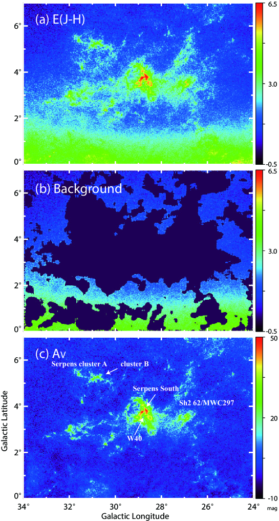
Figure 1.— (a) Color excess map of $E(J-H)$ of the Aquila Rift and Serpens molecular cloud complex generated by Dobashi (2011) and Dobashi et al. (2013). The fits data were downloaded from their website (http://darkclouds.u-gakugei.ac.jp/2MASS/download.html). (b) Same as (a), but the map is masked for small-scale structures to determine the background. (c) Extinction map of $A_{V}$ derived from the background-subtracted $E(J-H)$ map. The names of the regions discussed in the text are designated in the panel.

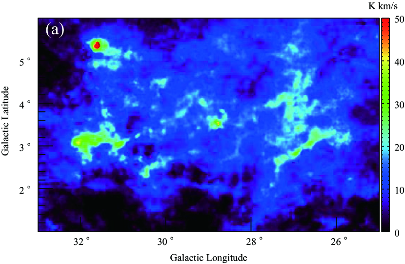
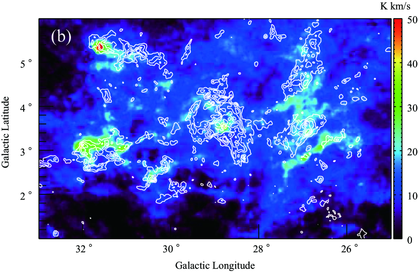
Figure 2.— (a) ¹²CO ($J=2-1$) total integrated intensity map in the velocity range from $V_{\rm LSR}=0$ km s^-1 to 20 km s^-1 toward the Aquila Rift and Serpens molecular cloud complexes. (b) Same as panel (a) but with contours of the 2MASS $A_{V}$ map. The contours start at 2.0 mag with intervals of 3.0 mag.

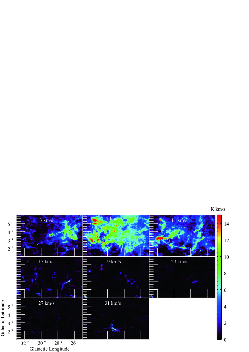
Figure 3.— ¹²CO ($J=2-1$) velocity channel maps toward the Aquila Rift and Serpens molecular cloud complexes. (Animations of the channel maps are available in the online journal.)

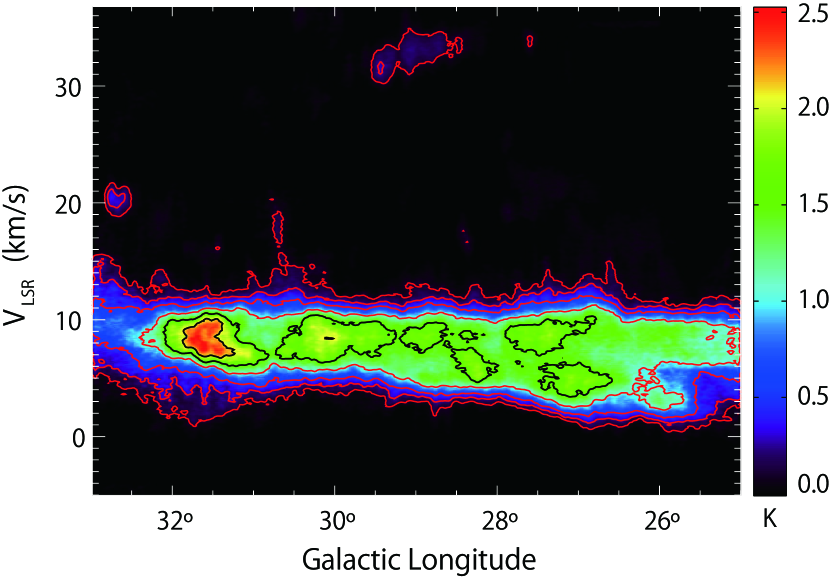
Figure 4.— ¹²CO ($J=2-1$) longitude-velocity diagram integrated over the entire Galactic latitude range observed ($1^{\circ}<b<6^{\circ}$). The contours are drawn at 0.1, 0.25, 0.5, 1.0, 1.5, 2.0, and 2.5 K.

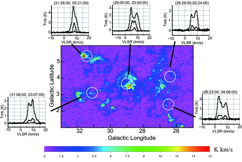
Figure 5.— CO line spectra at several positions. Three CO line spectra are averaged in the circles with radius of 20^′′. In each panel, the strongest, second strongest, and weakest lines are ¹²CO ($J=2-1$), ¹³CO ($J=2-1$), and C¹⁸O ($J=2-1$), respectively. The image is the ¹³CO ($J=2-1$) velocity integrated intensity map.

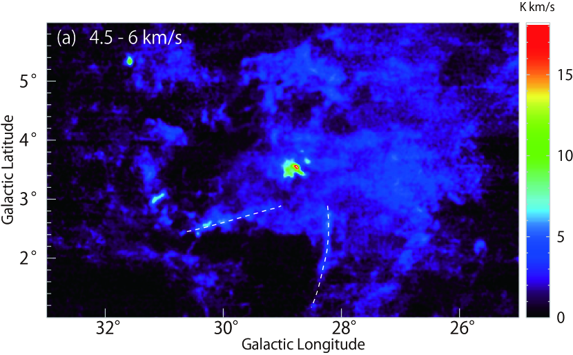
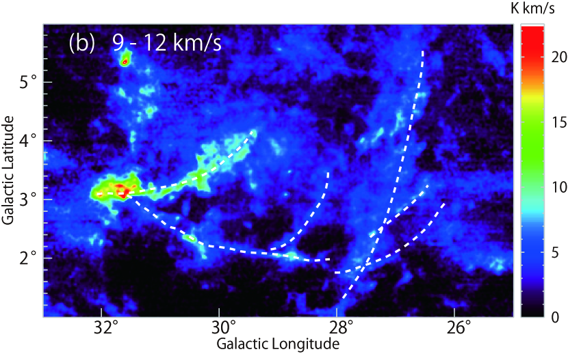
Figure 6.— Total intensity maps of the ¹²CO ($J=2-1$) emission integrated over (a) 4.5 $<V_{\rm LSR}<$6.0 km s^-1 and (b) $9.0<V_{\rm LSR}<12.0$ km s^-1.

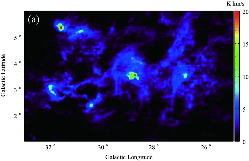
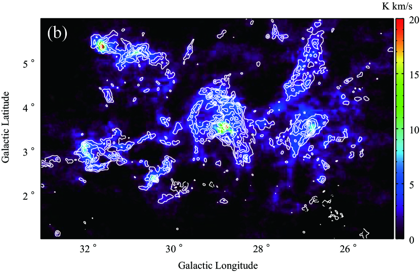
Figure 7.— (a) ¹³CO ($J=2-1$) total integrated intensity map in the velocity range from $V_{\rm LSR}=0$ km s^-1 to 20 km s^-1 toward the Aquila Rift and Serpens molecular cloud complexes. (b) Same as panel (a) but contours are the same as those of Figure 2b.

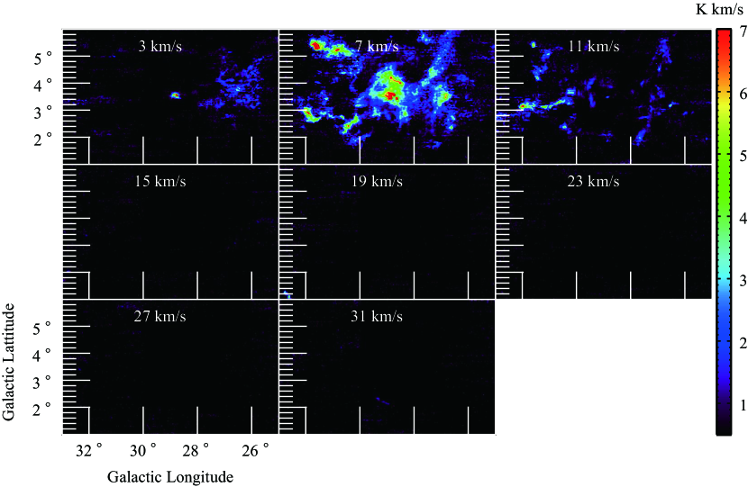
Figure 8.— ¹³CO ($J=2-1$) velocity channel maps toward the Aquila Rift and Serpens molecular cloud complexes. (Animations of the channel maps are available in the online journal.)

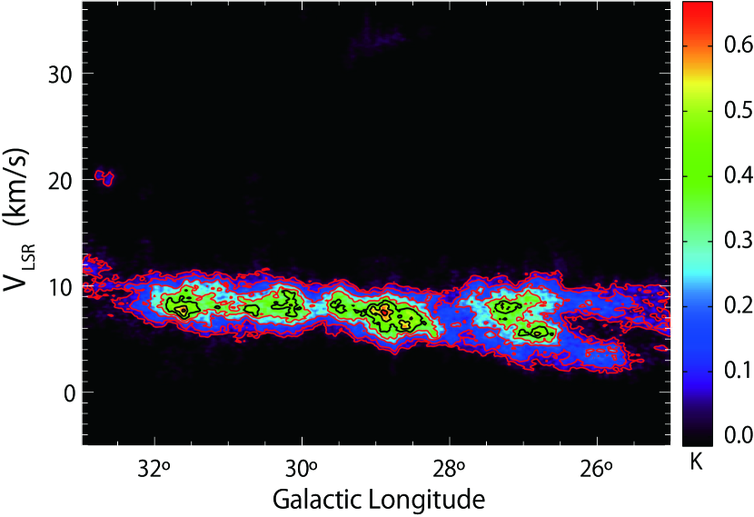
Figure 9.— ¹³CO ($J=2-1$) longitude-velocity diagram integrated over the entire Galactic latitude range observed ($1^{\circ}<b<6^{\circ}$). The contours are drawn at 0.05, 0.1, 0.2, 0.4, 0.5, and 0.6 K.

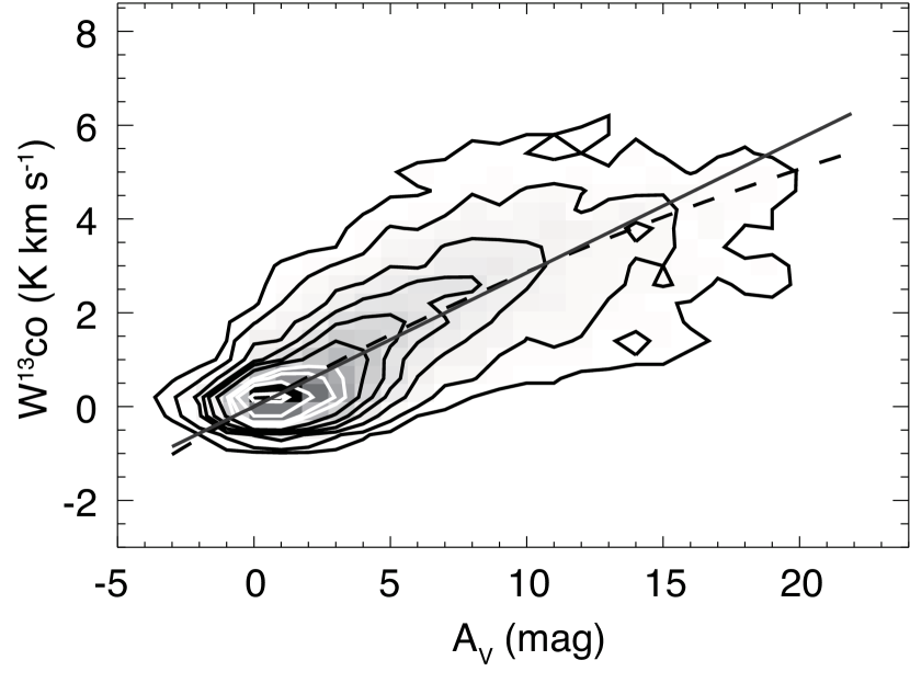
Figure 10.— The ¹³CO integrated intensity versus $A_{V}$. The solid and broken lines represent Equations (2) and (4) best fitting the relations, respectively. Contours are drawn to exclude 1, 5, 15, 25, 35, 45, 55, 65, 75, 85, and 95 $\%$ of the total data points (i.e., 99$\%$ of the data points are included within the lowest contour).

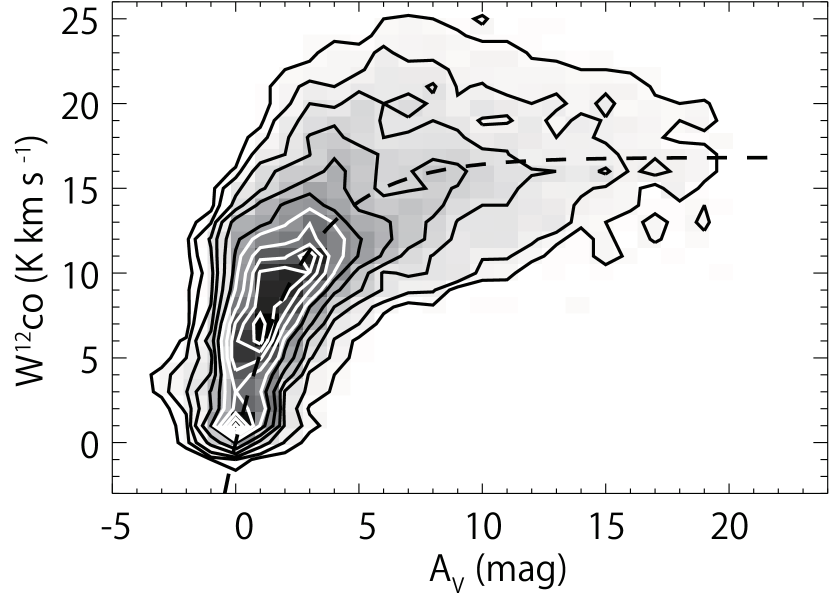
Figure 11.— The ¹²CO integrated intensity versus $A_{V}$. The relation is shown in the plot density. The broken line represents Equation (7) best fitting the relation. Contours are the same as in Figure 10.

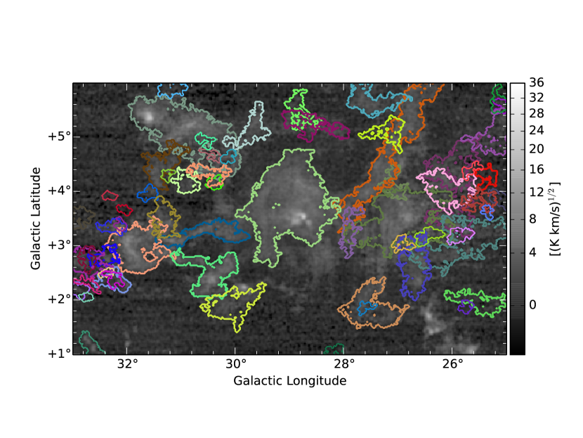
Figure 12.— Clouds identified by SCIME overlaid on the ¹³CO integrated intensity map. The clouds identified are enclosed by colored curves.

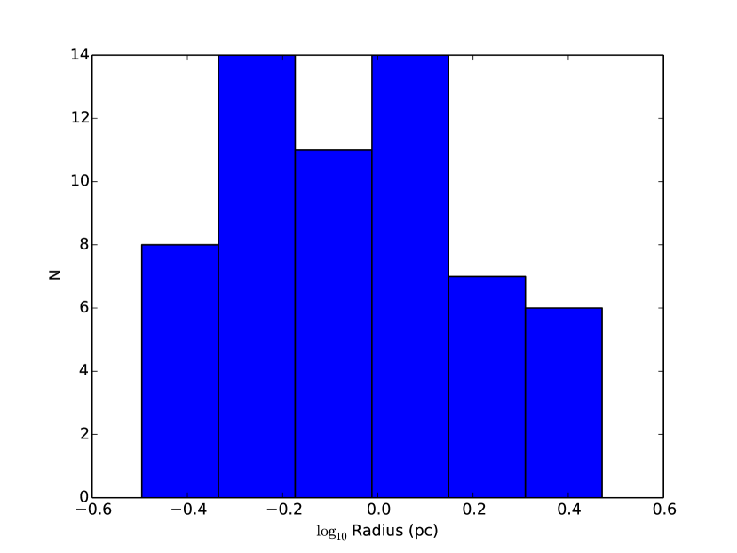
Figure 13.— Histogram of Cloud Radius.

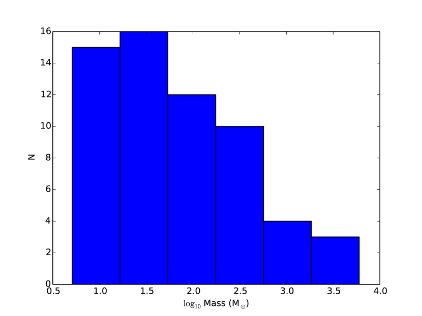
Figure 14.— Histogram of Cloud Mass.

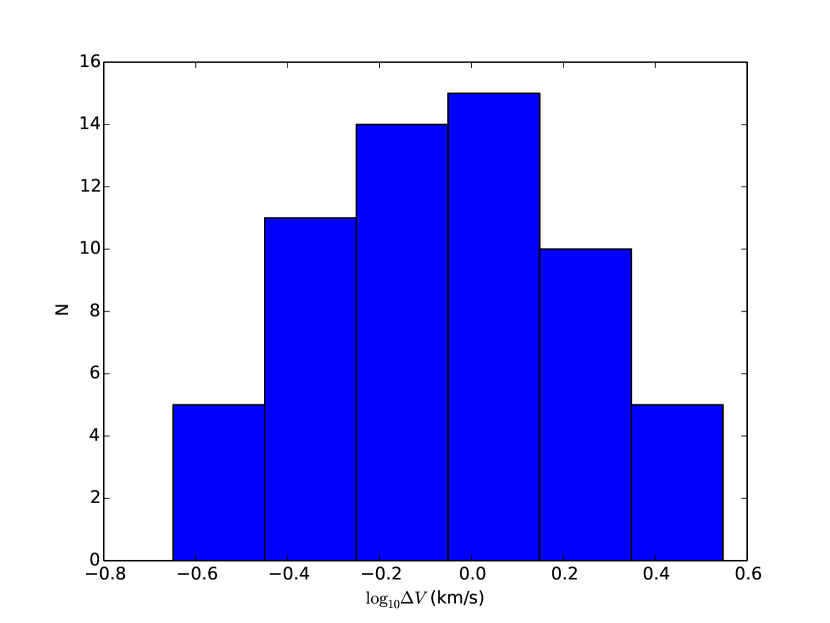
Figure 15.— Histogram of Line Widths.

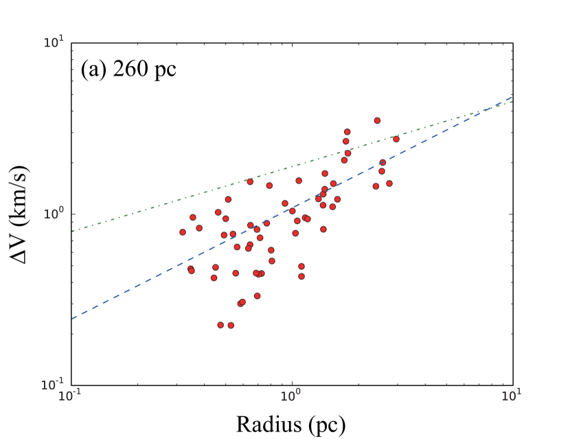
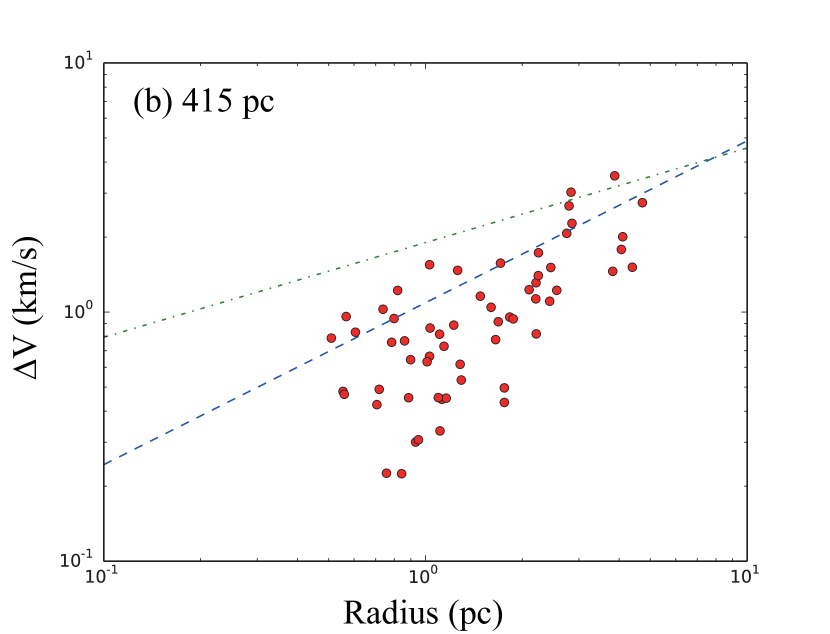
Figure 16.— Line-width-Radius Relations assuming a distance of (a) 216 pc and (b) 415 pc. The dashed and dashed-dotted lines are the line-width-radius relations derived by Heyer & Brunt (2004) and Larson (1981), respectively.

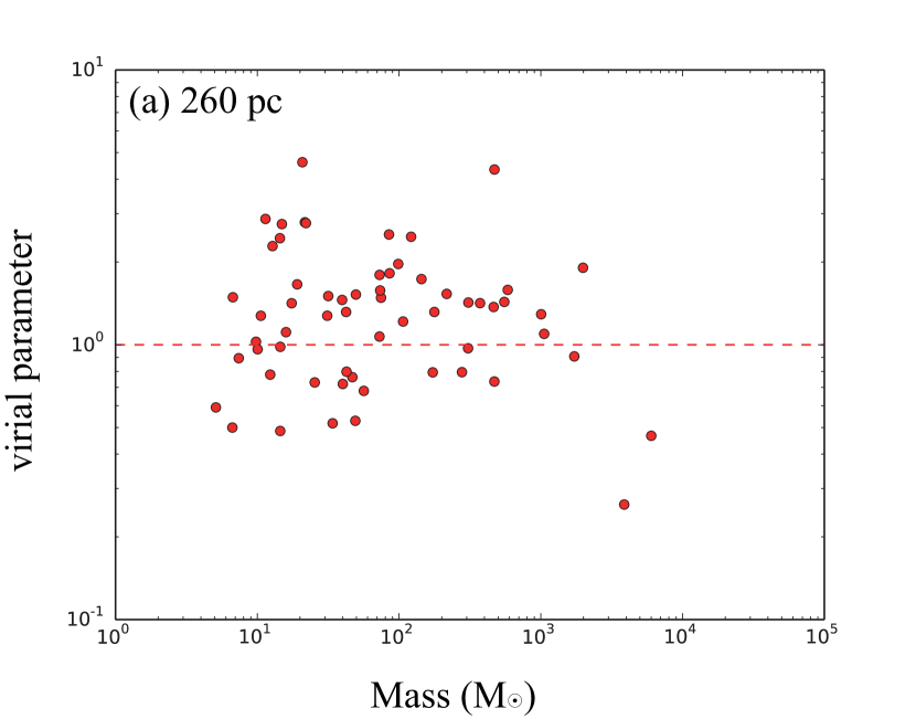
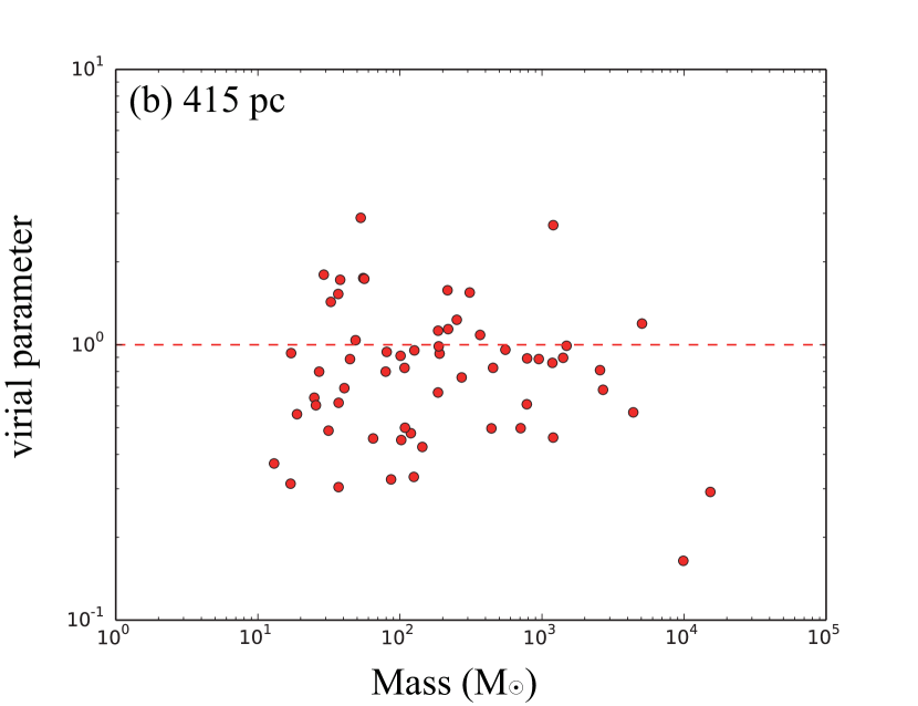
Figure 17.— Line-width-Radius Relations assuming a distance of (a) 216 pc and (b) 415 pc. The dashed lines indicate virial equilibrium.

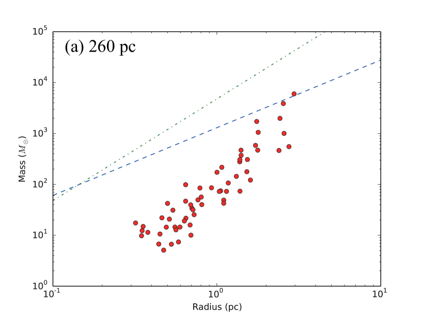
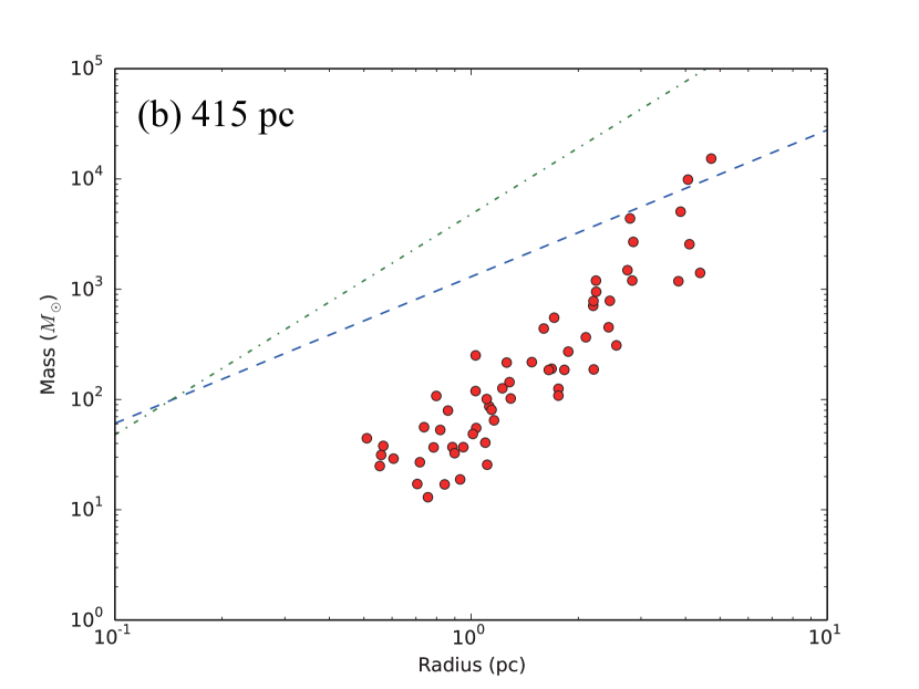
Figure 18.— Mass-Radius Relations assuming a distance of (a) 216 pc and (b) 415 pc. The dashed and dashed-dotted lines indicate Kauffmann et al. (2010)’s relation and Krumholz & McKee (2008)’s criteria for massive star formation, respectively.

Appendix A The noise levels of the data

The rms noise levels of the final ¹²CO, ¹³CO, and C¹⁸O maps varies from box to box, and were summarized in Tables A1, A2, and A3, respectively. The average noise levels are summarized in the last column of Table 1.

Table 4Rms noise levels of the ¹²CO map

	$l=33^{\circ}-32^{\circ}$	$l=32^{\circ}-31^{\circ}$	$l=31^{\circ}-30^{\circ}$	$l=30^{\circ}-29^{\circ}$	$l=29^{\circ}-28^{\circ}$	$l=28^{\circ}-27^{\circ}$	$l=27^{\circ}-26^{\circ}$	$l=26^{\circ}-25^{\circ}$
$b=6^{\circ}-5^{\circ}$	0.75	0.66	0.76	0.53	0.58	0.57	0.50	0.69
$b=5^{\circ}-4^{\circ}$	0.65	0.65	0.80	0.43	0.45	0.44	0.49	0.71
$b=4^{\circ}-3^{\circ}$	0.87	0.69	0.57	0.35	0.28	0.44	0.63	0.80
$b=3^{\circ}-2^{\circ}$	0.83	0.53	0.51	0.41	0.45	0.44	0.52	0.57
$b=2^{\circ}-1^{\circ}$	0.54	0.56	0.55	0.70	0.68	0.61	0.53	0.63

Note. — The rms noise levels are given in the brightness temperature scale (K). The velocity resolution is 0.079 km s^-1.

Table 5Rms noise levels of the ¹³CO map

	$l=33^{\circ}-32^{\circ}$	$l=32^{\circ}-31^{\circ}$	$l=31^{\circ}-30^{\circ}$	$l=30^{\circ}-29^{\circ}$	$l=29^{\circ}-28^{\circ}$	$l=28^{\circ}-27^{\circ}$	$l=27^{\circ}-26^{\circ}$	$l=26^{\circ}-25^{\circ}$
$b=6^{\circ}-5^{\circ}$	0.72	0.64	0.73	0.52	0.56	0.55	0.49	0.67
$b=5^{\circ}-4^{\circ}$	0.63	0.64	0.77	0.41	0.43	0.42	0.48	0.68
$b=4^{\circ}-3^{\circ}$	0.85	0.68	0.56	0.35	0.28	0.43	0.61	0.77
$b=3^{\circ}-2^{\circ}$	0.81	0.52	0.50	0.39	0.42	0.41	0.56	0.56
$b=2^{\circ}-1^{\circ}$	0.53	0.54	0.53	0.68	0.66	0.59	0.51	0.61

Note. — The rms noise levels are given in the brightness temperature scale (K). The velocity resolution is 0.083 km s^-1.

Table 6Rms noise levels of the C¹⁸O map

	$l=33^{\circ}-32^{\circ}$	$l=32^{\circ}-31^{\circ}$	$l=31^{\circ}-30^{\circ}$	$l=30^{\circ}-29^{\circ}$	$l=29^{\circ}-28^{\circ}$	$l=28^{\circ}-27^{\circ}$	$l=27^{\circ}-26^{\circ}$	$l=26^{\circ}-25^{\circ}$
$b=6^{\circ}-5^{\circ}$	0.73	0.64	0.73	0.52	0.56	0.55	0.49	0.67
$b=5^{\circ}-4^{\circ}$	0.64	0.64	0.77	0.41	0.43	0.41	0.48	0.68
$b=4^{\circ}-3^{\circ}$	0.84	0.68	0.56	0.34	0.28	0.43	0.60	0.78
$b=3^{\circ}-2^{\circ}$	0.81	0.52	0.50	0.39	0.42	0.41	0.55	0.55
$b=2^{\circ}-1^{\circ}$	0.53	0.54	0.53	0.68	0.65	0.58	0.50	0.61

Note. — The rms noise levels are given in the brightness temperature scale (K). The velocity resolution is 0.083 km s^-1.

References

- André et al. (2010) André, P., Menshchikov, A., Bontemps, S., et al. 2010, A&A, 518, L102
- Astropy Collaboration (2013) Astropy Collaboration, Robitaille, T. P., Tollerud, E. J., et al. 2013, A&A, 558, A33
- Bohlin et al. (1978) Bohlin, R. C., Savage, B. D., & Drake, J. F. 1978, ApJ, 224, 132
- Bolatto et al. (2013) Bolatto, A. D., Wolfire, M., & Leroy, A. K. 2013, ARA&A, 51, 207
- Colombo et al. (2015) Colombo, D., Rosolowsky, E., Ginsburg, A., Duarte-Cabral, A., & Hughes, A. 2015, MNRAS, 454, 2067
- Dame & Thaddeus (1985) Dame, T. M. & Thaddeus, P., 1985, ApJ, 297, 751
- Dame et al. (1987) Dame, T. M., Ungerechts, H., Cohen, R. S. et al., 1987, ApJ, 322, 706
- Dzib et al. (2010) Dzib, S., Loinard, L., Mioduszewski, A. J., et al. 2010, ApJ, 718, 610
- Dobashi et al. (2005) Dobashi, K., Uehara, H., Kandori, R., Sakurai, T., Kaiden, M., Umemoto, T., & Sato, F. 2005, PASJ, 57, S1
- Dobashi (2011) Dobashi, K. 2011, PASJ, 63, S1
- Dobashi et al. (2013) Dobashi, K., Marshall D. J., Shimoikura, T., & Bernard, J.-Ph. 2013, PASJ, 65, 31
- Drew et al. (1997) Drew, J. E., Busfield, G., Hoare, M. G., Murdoch, K. A., Nixon, C. A., Oudmaijer, R. D. 1997, MNRAS, 286, 538
- Duarte-Cabral et al. (2011) Duarte-Cabral, A., Dobbs, C. L., Peretto, N., & Fuller, G. A. 2011, A&A, 528, 50
- Eiroa et al. (2008) Eiroa, C., Djupvik, A. A., & Casali, M. M. 2008, in Handbook of Star Forming Regions Vol. II. p.693
- Frisch (1998) Frisch, P.C., 1998, in IAU Colloq. 166, The Local Bubble and Beyond, ed. D. Breitschwerdt, M. Freyberg & Trumper (Berlin: Springer), p. 269
- Heyer & Brunt (2004) Heyer, M. H., & Brunt, C. M. 2004, ApJ, 615, L45
- Hillenbrand et al. (1992) Hillenbrand, L. A., Strom, S. E., Vrba, F. J., Keene, J. 1992, ApJ, 397, 613
- Kawamura et al. (1999) Kawamura, A., Onishi, T., Mizuno, A. et al. 1999, PASJ, 51, 851
- Kauffmann et al. (2010) Kauffmann, J., Pillai, T., Shetty, R., Myers, P. C., & Goodman, A. A. 2010, ApJ, 716, 433
- Kirk et al. (2013) Kirk, H., Myers, P. C., Bourke, T. L., et al. 2013, ApJ, 766, 115
- Konyves et al. (2015) Konyves, V., André, P., Men’shchikov, A., et al. 2015, A&A, 584, 91
- Krumholz & McKee (2008) Krumholz, M. R., & McKee, C. F. 2008, Nature, 451, 28
- Larson (1981) Larson, R. B. 1981, MNRAS, 194, 809
- Lin et al. (2016) Lin, S.-J., Shimajiri, Y., Hara, C., et al. 2016, ApJ, 826, 193
- McMullin et al. (2000) Mcmullin, J.P., Mundy, L. G., Black, G. A., et al., 2000, ApJ, 536, 845
- Gutermuth et al. (2008) Gutermuth, R. A., Bourke, T. L., Allen, L. E., et al. ApJ, 2008, 673, L151
- Maruta et al. (2010) Maruta, H., Nakamura, F., Nishi, R., et al., 2010, ApJ, 714, 680
- Maury et al. (2011) Maury, A., P. André, Men’shchikov, A., Konyves, V., & Bontemps, S. 2011, A&A, 535, 77
- Nakamura et al. (2011) Nakamura, F., Sugitani, K., Shimajiri, Y. et al. 2011, ApJ, 737, 56
- Nakamura et al. (2014) Nakamura, F., Sugitani, K., Tanaka, T., et al. 2014, ApJ, 791, 23
- Onishi et al. (2013) Onishi, T., Nishimura, A., Ota, Y., et al. 2013, PASJ, 65,78
- Pineda et al. (2010) Pineda, J. L., Goldsmith, P. F., Chapman, N., et al. 2010, ApJ, 721, 686
- Plunkett et al. (2015) Plunkett, A. L., Arce, H., Corder, S. A., et al. 2015, ApJ, 803, 22
- Prato et al. (2008) Prato, L., Rice, E. L., & Dame, T. M. 2008, in Handbook of Star Forming Regions Vol. I.
- Reike & Lebofsky (1985) Reike, G. H., & Lebofsky, M. J. 1985, ApJ, 288, 618
- Rosolowsky et al. (2008) Rosolowsky, E., Pineda, J. E., Kauffmann, J., & Goodman, A. A. 2008, ApJ, 679, 1338
- Rodney & Reipurth (2008) Rodney, S. A. & Reipurth, B. 2008, Handbook of Star Forming Regions, Volume II, 693
- Shetty et al. (2012) Shetty, R., Beaumont, C. N., Burton, M. G., et al. 2012, MNRAS, 425, 720
- Shimoikura et al. (2015) Shimoikura, T., Dobashi, K., Nakamura, F., et al. 2015, ApJ, 806, 201
- Sugitani et al. (2011) Sugitani, K., Nakamura, F., Watanabe, M., et al. 2011, ApJ, 734, 63
- Tanaka et al. (2013) Tanaka, T., Nakamura, F., Awazu, Y., et al. 2013, ApJ, 778, 34
- Van der Tak et al. (2007) Van der Tak, F. F. S., Black, J. H., Scholer, F. L., Jansen, D. J., van Dischoeck, E. F. 2007, A&A, 468, 627