Design and Analysis of Sparsifying Dictionaries for FIR MIMO Equalizers

Abstract

In this paper, we propose a general framework that transforms the problems of designing sparse finite-impulse-response linear equalizers and non-linear decision-feedback equalizers, for multiple antenna systems, into the problem of sparsest-approximation of a vector in different dictionaries. In addition, we investigate several choices of the sparsifying dictionaries under this framework. Furthermore, the worst-case coherences of these dictionaries, which determine their sparsifying effectiveness, are analytically and/or numerically evaluated. Moreover, we show how to reduce the computational complexity of the designed sparse equalizer filters by exploiting the asymptotic equivalence of Toeplitz and circulant matrices. Finally, the superiority of our proposed framework over conventional methods is demonstrated through numerical experiments.

I Introduction

In single-carrier transmission over broadband channels, long finite impulse response (FIR) equalizers are typically implemented at high sampling rates to combat the channel’s frequency selectivity. However, implementation of such equalizers can be prohibitively expensive as the design complexity of FIR equalizers grows proportional to the square of the number of nonzero taps in the filter. Sparse equalization, where only few nonzero coefficients are employed, is a widely-used technique to reduce complexity at the cost of a tolerable performance loss. Nevertheless, reliably determining the locations of these nonzero coefficients is often very challenging.

Recently, sparse equalizers have been investigated both from practical [1, 2] and theoretical [3, 4] perspectives to reduce the implementation cost of long FIR filters. In [1], a direct-adaptive scheme is used for designing sparse FIR filters for multi-channel turbo equalization in underwater acoustic communications. However, the proposed approach is limited to the case of a single-input linear equalizer. In [2], the authors exploit sparsity in ionospheric High Frequency (HF) communications systems by formulating equalization at the HF receiver as a sparse signal recovery problem. However, the resulting solution is not exactly sparse and an additional heuristic optimization step is applied to further eliminate the small nonzero entries. In [3], a general optimization problem for designing a sparse filter is formulated that involves a quadratic constraint on filter performance. Nonetheless, the number of iterations of the proposed algorithm becomes large as the desired sparsity level of the filter increases. In addition, the approach in [3] also involves inversion of a large matrix in the case of a long channel impulse response (CIR). Sparse filters can also be designed using integer programming methods [4]. However, the design process can be computationally complex.

In [5], the number of nonzero coefficients is reduced by selecting only the significant taps of the equalizer. Nonetheless, knowledge of the complete equalizer tap vector is still required, which increases the computational complexity. In [6], an $\ell_{1}$-norm minimization problem is formulated to design a sparse filter. However, since the resulting filter taps are not exactly sparse, a thresholding step is required to force some of the nonzero taps to $0$. An algorithm, called sparse chip equalizer, for finding the locations of sparse equalizer taps is presented in [7], but this approach assumes that the CIR itself is sparse.

In [8], an algorithm for designing a decision feedback equalizer (DFE) is proposed, but the feedforward filter (FFF) taps are designed to only equalize the channel taps having the highest signal-to-noise ratios (SNRs). The number of the FFF and feedback filter (FBF) taps are optimized in [9]. However, since no sparsity constraints are imposed on the design, the final solution is not guaranteed to have low implementation complexity. In [10], multiple-input multiple-output (MIMO) equalizers are optimally designed; however, the design complexity of the equalizers is proportional to the product of the number of input and output streams. The sparsity of some channel models, e.g., [11] and [12], is exploited in [13] to further reduce the number of equalizer taps. In [14], a new matching-pursuit-type algorithm for DFE adaptation is proposed and the direct-adaptive sparse equalization problem is investigated from a compressive sensing perspective. However, the algorithm in [14] exploits inherent channel characteristics such as sparsity, i.e., the CIR is assumed to have a large delay spread with only few dominant taps. In [15], a framework for designing sparse FIR equalizers is proposed. Using greedy algorithms, the proposed framework achieved better performance than just choosing the largest taps of the minimum mean square error (MMSE) equalizer, as in [5]. However, this approach involves inversion of large matrices and Cholesky factorization, whose computational cost could be large for channels with large delay spreads. In addition, no theoretical sparse approximation guarantees are provided.

In this paper, we develop a general framework for the design of sparse FIR MIMO linear equalizers (LEs) and DFEs that transforms the original problem into one of sparse approximation of a vector using different dictionaries. The developed framework trivially specializes to the case of single-input single-input (SISO) systems. In both cases, the framework can then be used to find the sparsifying dictionary that leads to the sparsest FIR filter subject to an approximation constraint. Moreover, we investigate the coherence of the sparsifying dictionaries that we propose as part of our analysis and identify one dictionary that has small coherence. Then, we use simulations to validate that the dictionary with the smallest coherence results in the sparsest FIR design. For all design problems, we propose reduced-complexity sparse FIR filter designs by exploiting the asymptotic equivalence of Toeplitz and circulant matrices, where the matrix factorizations involved in our design analysis can be carried out efficiently using the fast Fourier transform (FFT) and inverse FFT with negligible performance loss as the number of filter taps increases. Finally, numerical results demonstrate the significance of our approach compared to conventional sparse filter designs, e.g., in [16] and [5], in terms of both performance and computational complexity.

The remainder of this paper is organized as follows. After introducing the system model in Section II, we formulate the sparse equalization problem for MIMO LEs and DFEs systems in Section III. Our proposed unified framework is described in Section IV. Then, numerical results are presented in Section V. Finally, the paper is concluded in Section VI.

Notations: We use the following standard notation in this paper: $\mbox{$\boldsymbol{I}$}_{N}$ denotes the identity matrix of size $N$. Upper- and lower-case bold letters denote matrices and vectors, respectively. Underlined upper-case bold letters, e.g., $\boldsymbol{\underline{X}}$, denote frequency-domain vectors. The notations $(.)^{-1},\,(.)^{*},\,(.)^{T}\mbox{ and }\,(.)^{H}$ denote the matrix inverse, the matrix (or element) complex conjugate, the matrix transpose and the complex-conjugate transpose operations, respectively. E$\left[.\right]$ denotes the expected value operator. $\left\|.\right\|_{\ell}$ and $\left\|.\right\|_{F}$ denote the $\ell$-norm and Frobenius norm, respectively. $\otimes$ denotes the Kronecker product of matrices. The components of a vector starting from $k_{1}$ and ending at $k_{2}$ are given as subscripts to the vector separated by a colon, i.e., $\boldsymbol{x}_{k_{1}:k_{2}}.$

Table I: Channel equalization notation and key matrices used in this paper.

Notation	Meaning	Size
$\boldsymbol{H}$	Channel matrix	$n_{o}N_{f}\times n_{i}\left(N_{f}+v\right)$
$\boldsymbol{R}_{xx}$	Input auto-correlation matrix	$n_{i}\left(N_{f}+v\right)\times\,\!\,n_{i}\left(N_{f}+v\right)$
$\boldsymbol{R}_{xy}$	Input-output cross-correlation matrix	$n_{i}\left(N_{f}+v\right)\times n_{o}\left(N_{f}\right)$
$\boldsymbol{R}_{yy}$	Output auto-correlation matrix	$n_{o}N_{f}\times n_{o}N_{f}$
$\boldsymbol{R}_{nn}$	Noise auto-correlation matrix	$n_{o}N_{f}\times n_{o}N_{f}$
$\boldsymbol{R}^{\perp}$	$\triangleq\boldsymbol{R}_{xx}-\boldsymbol{R}_{xy}\boldsymbol{R}_{yy}^{-1}\boldsymbol{R}_{yx}$	$n_{i}\left(N_{f}+v\right)\times\,\,\!n_{i}\left(N_{f}+v\right)$
$\boldsymbol{W}$	FFF matrix cofficients	$n_{o}N_{f}\times n_{i}$
$\boldsymbol{B}$	FBF matrix cofficients	$n_{i}\left(N_{f}+v\right)\times n_{i}$

II System Model

We consider a linear time-invariant MIMO inter-symbol interference (ISI) channel with $n_{i}$ inputs and $n_{o}$ outputs (the key matrices used in this paper are summarized in Table I). The received sample at the $r^{th}$ output antenna $\left(1\leq r\leq n_{o}\right)$ at time $k$ can be expressed as

$$y_{k}^{\left(r\right)}=\sum_{i=1}^{n_{i}}\sum_{l=0}^{v^{\left(i,r\right)}}\boldsymbol{h}_{l}^{\left(i,r\right)}\boldsymbol{x}_{k-l}^{\left(i\right)}+n_{k}^{\left(r\right)}\,,$$ (1)

where $y_{k}^{\left(r\right)}$ is the $r^{th}$ channel output, $\boldsymbol{h}_{l}^{\left(i,r\right)}$ is the CIR between the $i^{th}$ input and the $r^{th}$ output whose memory length is $v^{\left(i,r\right)}$, and $n_{k}^{\left(r\right)}$ is the noise at the $r^{th}$ output antenna. The received samples from all $n_{o}$ channel outputs at sample time $k$ are grouped into a $n_{o}\times 1$ column vector $\boldsymbol{y}_{k}$ as follows:

$$\boldsymbol{y}_{k}=\sum_{l=0}^{v}\boldsymbol{H}_{l}\boldsymbol{x}_{k-l}+\boldsymbol{n}_{k}\,,$$ (2)

where $\boldsymbol{H}_{l}$ is the $l^{th}$ channel matrix coefficient of dimension $\left(n_{o}\times n_{i}\right)$, and $\boldsymbol{x}_{k-l}$ is size $n_{i}\times 1$ input vector at time $k-l$. The parameter $v$ is the maximum order of all of the $n_{o}n_{i}$ CIRs, i.e., $v=\max_{(i,r)}v^{(i,r)}$. Over a block of $N_{f}$ output samples, the input-output relation in (2) can be written compactly as

$$\boldsymbol{y}_{k:k-N_{f}+1}=\boldsymbol{H}\,\boldsymbol{x}_{k:k-N_{f}-v+1}+\boldsymbol{n}_{k:k-N_{f}+1}\,,$$ (3)

where $\boldsymbol{y}_{k:k-N_{f}+1},\,\boldsymbol{x}_{k:k-N_{f}-v+1}$ and $\boldsymbol{n}_{k:k-N_{f}+1}$ are column vectors grouping the received, transmitted and noise samples, respectively. Recall that $\boldsymbol{y}_{k:k-N_{f}+1}$ is a vector of length $n_{o}N_{f}$, i.e., $\boldsymbol{y}=\left[\begin{array}[]{cccc}\boldsymbol{y}_{k}&\boldsymbol{y}_{k-1}&\ldots&\boldsymbol{y}_{k-N_{f}+1}\end{array}\right]^{T}$. Additionally, $\boldsymbol{H}$ is a block Toeplitz matrix whose first block row is formed by $\{\boldsymbol{H}_{l}\}_{l=0}^{l=v}$ followed by zero matrices. It is useful, as will be shown in the sequel, to define the output auto-correlation and the input-output cross-correlation matrices based on the block of length $N_{f}$. Using (3), the $n_{i}(N_{f}+v)\times n_{i}(N_{f}+v)$ input correlation and the $n_{o}N_{f}\times n_{o}N_{f}$ noise correlation matrices are, respectively, defined by $\boldsymbol{R}_{xx}\triangleq E\left[\boldsymbol{x}_{k:k-N_{f}-v+1}\boldsymbol{x}_{k:k-N_{f}-v+1}^{H}\right]\mbox{ and }\boldsymbol{R}_{nn}\triangleq E\left[\boldsymbol{n}_{k:k-N_{f}+1}\boldsymbol{n}_{k:k-N_{f}+1}^{H}\right]$. Both the input and noise processes are assumed to be white; hence, their auto-correlation matrices are assumed to be (multiples of) the identity matrix, i.e., $\boldsymbol{R}_{xx}=\boldsymbol{I}_{n_{i}(N_{f}+v)}$ and $\boldsymbol{R}_{nn}=\frac{1}{SNR}\boldsymbol{I}_{n_{o}N_{f}}$. Moreover, the output-input cross-correlation and the output auto-correlation matrices are, respectively, defined as

$$\!\!\boldsymbol{R}_{yx} \!\!\triangleq \!\!E\left[\!\boldsymbol{y}_{k:k-N_{f}+1}\boldsymbol{x}_{k:k-N_{f}-v+1}^{H}\!\right]\!\!=\boldsymbol{H}\boldsymbol{R}_{xx}\,,\,\mbox{and}$$ (4)

$$\!\!\boldsymbol{R}_{yy} \!\!\triangleq \!\!E\left[\!\boldsymbol{y}_{k:k-N_{f}+1}\boldsymbol{y}_{k:k-N_{f}+1}^{H}\!\right]\!\!=\!\boldsymbol{H}\boldsymbol{R}_{xx}\boldsymbol{H}^{H}\!\!+\!\boldsymbol{R}_{nn}.$$ (5)

III Sparse FIR Equalization

In this section, we formulate the sparse FIR equalizer design problems for MIMO LEs and DFEs.

III-A Sparse FIR MIMO LE

The received samples are passed through a MIMO FIR filter of length $n_{o}N_{f}$ for equalization. Define the $k^{th}$ equalization error sample vector in the MIMO setting as [10]

$$\boldsymbol{e}_{k}=\left[\begin{array}[]{ccccc}e_{k,1}&e_{k,2}&\ldots&\ldots&e_{k,n_{i}}\end{array}\right]^{T}\,,$$ (6)

where $e_{k,i}$ is the equalization error of the $i^{th}$ input stream. The resulting $k^{th}$ error sample for the $i^{th}$ input stream can be expressed as [10]

$$e_{k,i}=x_{k-\Delta,i}-\hat{x}_{k}=x_{k-\Delta,i}-\boldsymbol{w}_{i}^{H}\boldsymbol{y}_{k:k-N_{f}+1}\,,$$ (7)

where $\Delta$ is the decision delay, typically $0\leq\Delta\leq N_{f}+v-1$, and $\boldsymbol{w}_{i}$ denotes the equalizer taps vector for the $i^{th}$ input stream whose dimension is $n_{o}N_{f}\times 1$. The MSE of $e_{k,i}$, i.e., $\xi_{i}\left(\boldsymbol{w}_{i}\right)$, for the $i^{th}$ input stream can be written as

$$\xi_{i}\left(\boldsymbol{w}_{i}\right)=\xi_{m,i}+\underbrace{(\boldsymbol{w}_{i}-\boldsymbol{R}_{yy}^{-1}\boldsymbol{r}_{\Delta,i})^{H}\boldsymbol{R}_{yy}(\boldsymbol{w}_{i}-\boldsymbol{R}_{yy}^{-1}\boldsymbol{r}_{\Delta,i})}_{\triangleq\xi_{ex,i}(\boldsymbol{w}_{i})}\,,$$ (8)

where $\xi_{m,i}\triangleq\varepsilon_{x,i}-\boldsymbol{r}_{\Delta,i}^{H}\boldsymbol{R}_{yy}^{-1}\boldsymbol{r}_{\Delta,i}$, $\varepsilon_{x,i}\triangleq E\left[x_{k-\Delta,i}^{2}\right]$, $\boldsymbol{r}_{\Delta,i}^{H}=\boldsymbol{R}_{yx}\boldsymbol{1}_{\Delta,i}$, and $\boldsymbol{1}_{\Delta,i}$ is the $(n_{i}\Delta+i)$-th column of $\boldsymbol{I}_{n_{i}(N_{f}+v)}$. Clearly, the optimum choice for $\boldsymbol{w}_{i}$, in the MMSE sense, is the complex non-sparse solution: $\boldsymbol{w}_{opt,i}=\boldsymbol{R}_{yy}^{-1}\boldsymbol{r}_{\Delta,i}.$ However, in general, $\boldsymbol{w}_{opt.i}$ is not sparse and its implementation complexity increases proportional to $(n_{o}N_{f})^{2}$, which can be computationally expensive [17]. However, any choice for $\boldsymbol{w}_{i}$ other than $\boldsymbol{w}_{opt,i}$ increases $\xi_{i}(\boldsymbol{w}_{i})$, which results in performance loss. This suggests that we can use the excess error $\xi_{ex,i}(\boldsymbol{w}_{i})$ as a design constraint to achieve a desirable performance-complexity tradeoff. Specifically, we formulate the following problem for the design of a sparse FIR MIMO LE

$$\widehat{\boldsymbol{w}}_{s,i} \triangleq \underset{\boldsymbol{w}_{i}\in\mathbb{C}^{n_{o}N_{f}}}{\mbox{arg}\mbox{min}}\,\,\left\|\boldsymbol{w}_{i}\right\|_{0}\,\,\,\,\mbox{subject to}\,\,\,\,\,\xi_{ex,i}(\boldsymbol{w}_{i})\leq\delta_{eq,i}\,,$$

where $\left\|\boldsymbol{w}_{i}\right\|_{0}$ is the number of nonzero elements in its argument and $\delta_{eq,i}$ can be chosen as a function of the noise variance. To solve (LABEL:eq:opt_prob1), we propose a general framework presented in the sequel to sparsely design FIR MIMO LEs such that the performance loss does not exceed a pre-specified limit. We conclude this section by pointing out that the setup in (LABEL:eq:opt_prob1) can be easily specialized to the case of sparse FIR SISO LEs.

III-B Sparse FIR MIMO DFE

The FIR MIMO-DFE consists of two filters: a FFF matrix [10]

$$\boldsymbol{W}^{H}\triangleq\left[\begin{array}[]{cccc}\boldsymbol{W}_{0}^{H}&\boldsymbol{W}_{1}^{H}&\ldots&\boldsymbol{W}_{N_{f}-1}^{H}\end{array}\right]\,,$$ (10)

with $N_{f}$ matrix taps $\boldsymbol{W}_{i}^{H}$, each of size $n_{o}\times n_{i}$, and a FBF matrix equal to

$$\widetilde{\boldsymbol{B}}^{H}=\left[\begin{array}[]{cccc}\widetilde{\boldsymbol{B}}_{0}^{H}&\widetilde{\boldsymbol{B}}_{1}^{H}&\ldots&\widetilde{\boldsymbol{B}}_{N_{b}}^{H}\end{array}\right]\,,$$ (11)

where each $\widetilde{\boldsymbol{B}}_{i}^{H}$ has $\left(N_{b}+1\right)$ taps with size of $n_{i}\times n_{i}$. Therefore, $\boldsymbol{W}_{i}$ and $\widetilde{\boldsymbol{B}}_{i}$ have the forms

$$\boldsymbol{W}_{i}=\left[\begin{array}[]{ccc}w_{i}^{\left(1,1\right)}&\ldots&w_{i}^{\left(1,n_{i}\right)}\\ \vdots&\ldots&\vdots\\ w_{i}^{\left(n_{o},1\right)}&&w_{i}^{\left(n_{o},n_{i}\right)}\end{array}\right]$$ (12)

$$\widetilde{\boldsymbol{B}}_{i}=\left[\begin{array}[]{ccc}b_{i}^{\left(1,1\right)}&\ldots&b_{i}^{\left(1,n_{i}\right)}\\ \vdots&\ldots&\vdots\\ b_{i}^{\left(n_{o},1\right)}&&b_{i}^{\left(n_{o},n_{i}\right)}\end{array}\right]$$ (13)

By defining the size $n_{i}\times n_{i}(N_{f}+v)$ matrix $\boldsymbol{B}^{H}=\left[\begin{array}[]{cc}\boldsymbol{0}_{n_{i}\times n_{i}\Delta}&\widetilde{\boldsymbol{B}}^{H}\end{array}\right]$, where $0\leq\Delta\leq N_{f}+v-1$ is the decision delay that satisfies the condition $\left(\Delta+N_{b}+1\right)=\left(N_{f}+v\right)$, it was shown in [10] that the MSE of the error vector at time $k$, i.e., $\boldsymbol{E}_{k}=\boldsymbol{B}^{H}\boldsymbol{x}_{k:k-N_{f}-v+1}-\boldsymbol{W}^{H}\boldsymbol{y}_{k:k-N_{f}+1}$, is given by [18, 19]

$$\!\!\!\xi\left(\boldsymbol{B},\boldsymbol{W}\right) \!\!\!=\!\!\! \underbrace{\mbox{ Trace}\left\{\boldsymbol{B}^{H}\boldsymbol{R}^{\perp}\boldsymbol{B}\vphantom{\boldsymbol{S}^{H}\boldsymbol{R}_{yy}}\right\}}_{\triangleq\,\xi_{m}\left(\boldsymbol{B}\right)}+\underbrace{\mbox{$\mbox{Trace}\left\{\boldsymbol{S}^{H}\boldsymbol{R}_{yy}\boldsymbol{S}\right\}$}}_{\triangleq\,\xi_{ex}(\boldsymbol{W},\boldsymbol{B})}\,,$$ (14)

where $\boldsymbol{R}^{\perp}\triangleq\boldsymbol{R}_{xx}-\boldsymbol{R}_{xy}\boldsymbol{R}_{yy}^{-1}\boldsymbol{R}_{yx}$ and $\boldsymbol{S}^{H}\triangleq\!\boldsymbol{W}^{H}\!\!-\!\!\boldsymbol{B}^{H}\boldsymbol{R}_{xy}\boldsymbol{R}_{yy}^{-1}.$ The second term of the MSE in (14) is equal to zero for the case of the optimum FFF matrix filter coefficients, i.e., $\boldsymbol{W}^{H}\!\!=\!\!\boldsymbol{B}^{H}\boldsymbol{R}_{xy}\boldsymbol{R}_{yy}^{-1}$, and the resulting MSE can then be expressed as follows $\left(\mbox{defining}\boldsymbol{\,R}^{\perp}\triangleq\boldsymbol{A}_{\perp}^{H}\boldsymbol{A}_{\perp}\right)$

$$\xi_{m}\left(\boldsymbol{B}\right) \!\!\!\!=\!\!\!\! \mbox{Trace}\left\{\boldsymbol{B}^{H}\boldsymbol{A}_{\perp}^{H}\boldsymbol{A}_{\perp}\boldsymbol{B}\right\}=\left\|\boldsymbol{A}_{\perp}\boldsymbol{B}\vphantom{A^{H}}\right\|_{F}^{2}$$ (16)

$$\!\!\!\!=\!\!\!\! \left\|\boldsymbol{A}_{\perp}\begin{array}[]{cccc}\boldsymbol{b}^{\left(1\right)}&\boldsymbol{A}_{\perp}\boldsymbol{b}^{\left(2\right)}&\ldots\ldots&\boldsymbol{A}_{\perp}\boldsymbol{b}^{\left(n_{i}\right)}\end{array}\right\|_{F}^{2}$$

$$= \!\!\!\left\|\boldsymbol{A}_{\perp}\!\!\begin{array}[]{c}\boldsymbol{b}^{\left(1\right)}\!\!\end{array}\right\|_{2}^{2}+\!\!\left\|\boldsymbol{A}_{\perp}\!\!\begin{array}[]{c}\boldsymbol{b}^{\left(2\right)}\!\!\end{array}\right\|_{2}^{2}\!+\cdots\cdots+\!\!\left\|\boldsymbol{A}_{\perp}\!\!\begin{array}[]{c}\boldsymbol{b}^{\left(n_{i}\right)}\!\!\end{array}\right\|_{2}^{2}$$ (20)

where $\boldsymbol{b}^{(i)}$ is the $i^{th}$ column of $\boldsymbol{B}$. Hence, to compute the FBF matrix filter taps $\boldsymbol{B}$ that minimize $\xi_{m}\left(\boldsymbol{B}\right)$, we minimize $\xi_{m}\left(\boldsymbol{B}\right)$ under the identity tap constraint (ITC), i.e., we restrict $\boldsymbol{B}_{0}$ to be equal to the identity matrix, i.e., $\boldsymbol{B}_{0}=\boldsymbol{I}_{n_{i}}$. Towards this goal, we rewrite $\xi_{m}\left(\boldsymbol{B}\right)$ as follows

$$\xi_{m}\left(\boldsymbol{B}\right)=\sum_{i=1}^{n_{i}}\left\|\boldsymbol{A}_{\perp}^{(:\setminus n_{i}\Delta+i)}\begin{array}[]{c}\boldsymbol{b}^{\left(i\setminus n_{i}\Delta+i\right)}+\boldsymbol{a}_{n_{i}\Delta+i}\end{array}\right\|_{2}^{2}\,,$$ (22)

where $\boldsymbol{A}_{\perp}^{(:\setminus n_{i}\Delta+i)}$ is formed by all columns of $\boldsymbol{A}_{\perp}$ except the $\left(n_{i}\Delta+i\right)^{th}$ column, i.e., $\boldsymbol{a}_{n_{i}\Delta+i}$, and $\boldsymbol{b}^{\left(i\setminus n_{i}\Delta+i\right)}$ is formed by all elements of $\begin{array}[]{c}\boldsymbol{b}^{\left(i\right)}\end{array}$ except the $\left(n_{i}\Delta+i\right)^{th}$ entry that is forced to have unit value. Then, we formulate the following problem for the design of sparse FBF matrix filter taps $\boldsymbol{B}$

$$\begin{array}[]{c}\,\,\,\widehat{\boldsymbol{b}}^{\left(i\setminus n_{i}\Delta+i\right)}\triangleq\underset{}{\mbox{\mbox{arg}\mbox{min}}}\,\left\|\boldsymbol{b}^{\left(i\setminus n_{i}\Delta+i\right)}\right\|_{0}\,\,\,\,\,\,\mbox{subject to}\\ \left\|\boldsymbol{A}_{\perp}^{(:\setminus n_{i}\Delta+n_{i})}\begin{array}[]{c}\boldsymbol{b}^{\left(i\setminus n_{i}\Delta+i\right)}+\boldsymbol{a}_{n_{i}\Delta+i}\mbox{\!\!\!}\end{array}\right\|_{2}^{2}\leq\gamma_{eq,i}\,,\end{array}$$ (23)

where $\widehat{\boldsymbol{b}}^{\left(.\right)}$ is the estimate of $\boldsymbol{b}^{\left(.\right)}$. Once $\widehat{\boldsymbol{b}}^{\left(i\setminus n_{i}\Delta+i\right)}\,,\forall i\in n_{i}$, is calculated, we insert the identity matrix $\boldsymbol{B}_{0}$ in the first location of $\boldsymbol{B}$ to form the sparse FBF matrix coefficients, i.e., $\boldsymbol{B}_{s}$. Note that $\gamma_{eq,i}$ can be used to provide different quality of service (QoS) levels, with small values assigned to users/streams that demand high QoS levels. Then, the optimum FFF matrix taps (in the MMSE sense) are determined from (14) to be

$$\boldsymbol{W}_{opt}=\boldsymbol{R}_{yy}^{-1}\boldsymbol{R}_{yx}\boldsymbol{B}_{s}=\boldsymbol{R}_{yy}^{-1}\boldsymbol{\overline{\beta}}\,.$$ (24)

Since $\boldsymbol{W}_{opt}$ is not sparse in general, we further propose a sparse implementation for the FFF matrix as follows. After computing $\boldsymbol{B}_{s}$, the MSE will be a function only of $\boldsymbol{W}$ and can be expressed as $\left(\mbox{defining}\boldsymbol{\,R}_{yy}\triangleq\boldsymbol{A}_{y}^{H}\boldsymbol{A}_{y}\right)$

$$\xi\left(\boldsymbol{B}_{s},\boldsymbol{W}\right) = \xi_{m}\left(\boldsymbol{B}_{s}\right)+$$ (25)

$$\mbox{Trace}\left\{\!\left(\!\boldsymbol{W}^{H}\!\!-\!\!\boldsymbol{\overline{\beta}}^{H}\boldsymbol{R}_{yy}^{-1}\right)\boldsymbol{A}_{y}^{H}\boldsymbol{A}_{y}\left(\!\boldsymbol{W}\!\!-\!\!\boldsymbol{R}_{yy}^{-1}\boldsymbol{\overline{\beta}}\right)\!\right\}$$

$$= \xi_{m}\left(\boldsymbol{B}_{s}\right)+\underbrace{\left\|\boldsymbol{A}_{y}\boldsymbol{W}-\boldsymbol{A}_{y}^{-H}\boldsymbol{\overline{\beta}}\right\|_{F}^{2}}_{\,\triangleq\,\xi_{ex}(\boldsymbol{W})}.$$

By minimizing $\xi_{ex}(\boldsymbol{W})$, we further minimize the MSE. This is achieved by a reformulation for $\xi_{ex}(\boldsymbol{W})$ to get a vector form of $\boldsymbol{W}$, as follows

$$\xi_{ex}(\overline{\boldsymbol{w}}_{f})=\left\|\underbrace{\left(\boldsymbol{I}_{n_{i}}\otimes\boldsymbol{A}_{y}^{H}\right)}_{\overline{\boldsymbol{\varPsi}}}\mbox{$\underbrace{\textbf{vec}\left(\boldsymbol{W}\right)\vphantom{\left(\boldsymbol{I}_{n_{i}}\otimes\boldsymbol{A}_{y}^{H}\right)}}_{\overline{\boldsymbol{w}}_{f}}-$$\underbrace{\textbf{vec}(\boldsymbol{A}_{y}^{-H}\boldsymbol{\overline{\beta}})\vphantom{\left(\boldsymbol{I}_{n_{i}}\otimes\boldsymbol{A}_{y}^{H}\right)}}_{\overline{\boldsymbol{a}}_{y}}$}\right\|_{2}^{2}\,,$$ (26)

where vec is an operator that maps a $n\times n$ matrix to a vector by stacking the columns of the matrix. Afterward, we solve the following problem to compute the FFF matrix filter taps

$$\widehat{\overline{\boldsymbol{w}}}_{s,f}\triangleq\underset{}{\mbox{\mbox{arg}\mbox{min}}}\,\left\|\overline{\boldsymbol{w}}_{f}\right\|_{0}\,\,\,\mbox{subject to}\,\,\,\,\,\,\xi_{ex}(\overline{\boldsymbol{w}}_{f})\leq\overline{\gamma}_{eq}\,,$$ (27)

where $\overline{\gamma}_{eq}>0$ is used to control the performance-complexity tradeoff. We conclude this section by noting that the FIR LEs follow as a special case of the FIR DFEs by setting $\boldsymbol{B}_{0}=\boldsymbol{I}_{n_{i}}$ and $\boldsymbol{B}_{\ell}=\boldsymbol{0}_{n_{i}\times n_{i}}$, $0\leq\ell\leq N_{b}$. In addition, the MSE matrix of DFE is a weighted version of that of the LE [21]. Moreover, the setup in (23) and (27) can be easily specialized to the case of sparse FIR SISO DFEs by setting the numbers of inputs and outputs to one.

IV Proposed Sparse Approximation Framework

Unlike earlier works, including the one by one of the co-authors [15], we provide a general framework for designing sparse FIR filters, for multiple antenna systems, that can be considered as the problem of sparse approximation using different dictionaries. Mathematically, this framework poses the FIR filter design problem as follows

$$\widehat{\boldsymbol{z}}_{s}\triangleq\underset{\boldsymbol{z}}{\mbox{\mbox{arg}\mbox{min}}}\,\left\|\boldsymbol{z}\right\|_{0}\,\,\,\mbox{subject to}\,\,\,\left\|\boldsymbol{K}\left(\boldsymbol{\varPhi}\boldsymbol{z}-\boldsymbol{d}\right)\right\|_{2}^{2}\leq\epsilon\,,$$ (28)

where $\boldsymbol{\varPhi}$ is the dictionary that will be used to sparsely approximate $\boldsymbol{d}$, while $\boldsymbol{K}$ is a known matrix and $\boldsymbol{d}$ is a known data vector, both of which change depending upon the sparsifying dictionary $\boldsymbol{\varPhi}$. Notice that $\widehat{\boldsymbol{z}}_{s}$ corresponds to one of the elements in $\{\widehat{\boldsymbol{w}}_{s,i},\,\widehat{\boldsymbol{b}}^{\left(.\right)},\,\widehat{\boldsymbol{\overline{w}}}_{s,f}\}$ and $\epsilon$ is the corresponding element in $\left\{\delta_{eq,i},\,\gamma_{eq,i},\,\overline{\gamma}_{eq}\right\}$. For all design problems, we perform the suitable transformation to reduce the problem to the one shown in (28). For instance, we complete the square in (LABEL:eq:opt_prob1) to reduce it to the formulation given in (28). Hence, one can use any factorization for $\boldsymbol{R}_{yy}$, e.g., in (8) or (14), and $\boldsymbol{R}^{\perp}$, e.g., in (14), to formulate a sparse approximation problem. Using the Cholesky or eigen decomposition for $\boldsymbol{R}_{yy},$ and $\boldsymbol{R}^{\perp}$, we will have different choices for $\boldsymbol{K}$, $\boldsymbol{\varPhi}$ and $\boldsymbol{d}$. For instance, by defining the Cholesky factorization [20] of $\boldsymbol{R}^{\perp}$, in (LABEL:eq:FBF_design_B), as $\boldsymbol{R}^{\perp}\triangleq\boldsymbol{L}_{\perp}\boldsymbol{L}_{\perp}^{H}$, or in the equivalent form $\boldsymbol{R}^{\perp}\triangleq\boldsymbol{P}_{\perp}\boldsymbol{\Sigma}_{\perp}\boldsymbol{P}_{\perp}^{H}=\boldsymbol{\varOmega}_{\perp}\boldsymbol{\varOmega}_{\perp}^{H}$ (where $\boldsymbol{L}_{\perp}$ is a lower-triangular matrix, $\boldsymbol{P}_{\perp}$ is a lower-unit-triangular (unitriangular) matrix and $\boldsymbol{\Sigma}_{\perp}$ is a diagonal matrix) and assuming $n_{i}=1$ (in which matrix $\boldsymbol{B}$ reduces to a vector $\boldsymbol{b}$), the problem in (28) can, respectively, take one of the forms shown below [22]

$$\underset{\boldsymbol{b}\in\mathbb{C}^{N_{f}+v-1}}{\mbox{min}}\,\,\left\|\boldsymbol{b}\right\|_{0}\mbox{\,\,\,\,\mbox{s.t. }\,\,\,\,$\left\|\left(\widetilde{\boldsymbol{L}}_{\perp}^{H}\,\widetilde{\boldsymbol{b}}+\boldsymbol{l}_{\Delta+1}\right)\right\|_{2}^{2}\leq\gamma_{eq,1}\,$,}$$ (29)

$$\underset{\boldsymbol{b}\in\mathbb{C}^{N_{f}+v-1}}{\mbox{min}}\,\,\left\|\boldsymbol{b}\right\|_{0}\mbox{\,\,\,\,\mbox{s.t. }\,\,\,\,$\left\|\left(\widetilde{\boldsymbol{\varOmega}}_{\perp}^{H}\,\widetilde{\boldsymbol{b}}+\boldsymbol{p}_{\Delta+1}\right)\right\|_{2}^{2}\leq\gamma_{eq,1}\,$.}$$ (30)

Note that $\widetilde{\boldsymbol{L}}_{\perp}^{H}$$\left(\widetilde{\boldsymbol{\varOmega}}_{\perp}^{H}\right)$ is formed by all columns of $\boldsymbol{L}_{\perp}^{H}$$\left(\boldsymbol{\varOmega}_{\perp}^{H}\right)$ except the $\left(\Delta+1\right)^{th}$ column, $\boldsymbol{l}_{\Delta+1}$$\left(\boldsymbol{p}_{\Delta+1}\right)$ is the $\left(\Delta+1\right)^{th}$ column of $\boldsymbol{L}_{\perp}^{H}$$\left(\boldsymbol{\varOmega}_{\perp}^{H}\right)$, and $\widetilde{\boldsymbol{b}}$ is formed by all entries of $\boldsymbol{b}$ except the $\left(\Delta+1\right)^{th}$ unity entry. Similarly, by writing the Cholesky factorization of $\boldsymbol{R}_{yy}$ in (8) as $\boldsymbol{R}_{yy}\triangleq\boldsymbol{L}_{y}\boldsymbol{L}_{y}^{H}$ or the eigen decomposition of $\boldsymbol{R}_{yy}$ as $\boldsymbol{R}_{yy}\triangleq\boldsymbol{U}_{y}\boldsymbol{D}_{y}\boldsymbol{U}_{y}^{H}$, we can formulate the problem in (28) as follows

$$\!\!\!\!\underset{\boldsymbol{w}_{i}\in\mathbb{C}^{n_{o}N_{f}}}{\mbox{min}}\left\|\boldsymbol{w}_{i}\right\|_{0}\mbox{\,\,\,\,\mbox{s.t. }\,\,\,\,$\left\|(\boldsymbol{L}_{y}^{H}\boldsymbol{w}_{i}-\boldsymbol{L}_{y}^{-1}\boldsymbol{r}_{\Delta,i})\right\|_{2}^{2}\leq\delta_{eq,i}\,$,}$$ (31)

$$\!\!\!\!\!\underset{\boldsymbol{w}_{i}\in\mathbb{C}^{n_{o}N_{f}}}{\mbox{min}}\!\!\left\|\boldsymbol{w}_{i}\right\|_{0}\mbox{\,\mbox{s.t. }\,$\left\|\boldsymbol{D}_{y}^{\frac{1}{2}}\boldsymbol{U}_{y}^{H}\boldsymbol{w}_{i}\!-\!\boldsymbol{D}_{y}^{-\frac{1}{2}}\boldsymbol{U}_{y}^{H}\boldsymbol{r}_{\Delta,i}\right\|_{2}^{2}\!\!\!\leq\!\delta_{eq,i},\,\mbox{and}\!\!$}$$ (32)

$$\!\!\!\!\!\!\underset{\boldsymbol{w}_{i}\in\mathbb{C}^{n_{o}N_{f}}}{\mbox{min}}\left\|\boldsymbol{w}_{i}\right\|_{0}\mbox{\,\,\,\,\mbox{s.t. }\,\,\,\,$\left\|\boldsymbol{L}_{y}^{-1}(\boldsymbol{R}_{yy}\boldsymbol{w}_{i}-\boldsymbol{r}_{\Delta,i})\right\|_{2}^{2}$$\leq$}\delta_{eq,i}.$$ (33)

Note that the sparsifying dictionaries in (31), (32) and (33) are $\boldsymbol{L}_{y}^{H}$, $\boldsymbol{D}_{y}^{\frac{1}{2}}\boldsymbol{U}_{y}^{H}$ and $\boldsymbol{R}_{yy}$, respectively. Furthermore, the matrix $\boldsymbol{K}$ is an identity matrix in all cases except in (33), where it is equal to $\boldsymbol{L}_{y}^{-1}$. Additionally, some possible sparsifying dictionaries that can be used to design a sparse FFF matrix filter, given in (27), are shown in Table II. It is worth pointing out that several other sparsifying dictionaries can be used to sparsely design FIR LEs, FBF and FFF matrix taps. In the interest of space, we have presented above few design problems with some possible choices for the sparsifying dictionaries and the other choices can be derived by applying suitable transformations to the given design problem.

Table II: Examples of different sparsifying dictionaries that can be used to design $\overline{\boldsymbol{w}}_{f}$ given in (27) .

Factorization Type	$\boldsymbol{K}$	$\boldsymbol{\varPhi}$	$\boldsymbol{d}$
$\boldsymbol{R}_{yy}=\boldsymbol{L}_{y}\boldsymbol{L}_{y}^{H}$	$\boldsymbol{I}$	$\boldsymbol{I}_{n_{i}}\otimes\boldsymbol{L}_{y}^{H}$	$\textbf{vec}(\boldsymbol{L}_{y}^{-1}\boldsymbol{\overline{\beta}})$
	$\boldsymbol{L}_{y}^{-1}$	$\boldsymbol{I}_{n_{i}}\otimes\boldsymbol{R}_{yy}$	$\textbf{vec}(\boldsymbol{\overline{\beta}})\vphantom{\boldsymbol{L}_{y}^{-H}}$
$\boldsymbol{R}_{yy}=\boldsymbol{P}_{y}\boldsymbol{\Lambda}_{y}\boldsymbol{P}_{y}^{H}$	$\boldsymbol{I}$	$\boldsymbol{I}_{n_{i}}\otimes\boldsymbol{\Lambda}_{y}^{\frac{1}{2}}\boldsymbol{P}_{y}^{H}$	$\textbf{vec}(\boldsymbol{\Lambda}_{y}^{-\frac{1}{2}}\boldsymbol{P}_{y}^{-1}\boldsymbol{\overline{\beta}})$
$\boldsymbol{R}_{yy}=\boldsymbol{U}_{y}\boldsymbol{D}_{y}\boldsymbol{U}_{y}^{H}$	$\boldsymbol{D}_{y}^{-\frac{1}{2}}\boldsymbol{U}_{y}^{H}$	$\boldsymbol{I}_{n_{i}}\otimes\boldsymbol{R}_{yy}$	$\textbf{vec}(\boldsymbol{\overline{\beta}})$
	$\boldsymbol{I}$	$\boldsymbol{I}_{n_{i}}\otimes\boldsymbol{D}_{y}^{\frac{1}{2}}\boldsymbol{U}_{y}^{H}$	$\textbf{vec}(\boldsymbol{D}_{y}^{-\frac{1}{2}}\boldsymbol{U}_{y}^{H}\boldsymbol{\overline{\beta}})$

So far, we have shown that the problem of designing sparse FIR filters can be cast into one of sparse approximation of a vector by a fixed dictionary. The general form of this problem is given by (28). To solve this problem, we use the well-known Orthogonal Matching Pursuit (OMP) greedy algorithm [23] that estimates $\widehat{\boldsymbol{z}}_{s}$ by iteratively selecting a set $S$ of the sparsifying dictionary columns (i.e., atoms $\boldsymbol{\phi}_{i}$’s) of $\boldsymbol{\varPhi}$ that are most correlated with the data vector $\boldsymbol{d}$ and then solving a restricted least-squares problem using the selected atoms. The OMP stopping criterion can be either a predefined sparsity level (number of nonzero entries) of $\boldsymbol{z_{s}}$ or an upper-bound on the norm of the residual error. We work with the latter case in our problem but change the stopping criterion from an upper-bound on the norm of the residual error to an upper-bound on the norm of “the Projected Residual Error (PRE)”, i.e., “$\boldsymbol{K}\times\left(\boldsymbol{\varPhi}\boldsymbol{z}-\boldsymbol{d}\right)$”. Note that the stopping criterion becomes a function of $\boldsymbol{K}$, and hence this value has to be passed to the OMP algorithm to determine $\epsilon$, i.e., $\widehat{\boldsymbol{z}}_{s}\triangleq\text{OMP}\left(\boldsymbol{\Phi},\boldsymbol{d},\boldsymbol{K},\epsilon\right)$. The computations involved in the OMP algorithm are well documented in the sparse approximation literature (e.g., [23]) and are omitted here for the sake of brevity.

Note that unlike conventional compressive sensing techniques [24], where the measurement matrix is a fat matrix, the sparsifying dictionary in our framework is either a tall matrix (fewer columns than rows) with full column rank as in (29) and (30) or a square one with full rank as in (31)–(33). However, OMP and similar methods can still be used for obtaining $\widehat{\boldsymbol{z}}_{s}$ if $\boldsymbol{R}_{yy}$ and $\boldsymbol{R}^{\perp}$ can be decomposed into $\boldsymbol{\Psi\varPsi^{H}}$ and the data vector $\boldsymbol{d}$ is compressible [25, 3].

Our next challenge is to determine the best sparsifying dictionary for use in our framework. We know from the sparse approximation literature that the sparsity of the OMP solution tends to be inversely proportional to the worst-case coherence $\mu\left(\boldsymbol{\varPhi}\right)$, where $\mu\left(\boldsymbol{\varPhi}\right)\triangleq\underset{i\neq j}{\mbox{max}}\frac{\left|\left\langle\phi_{i},\,\phi_{j}\right\rangle\right|\,}{\left\|\phi_{i}\right\|_{2}\left\|\phi_{j}\right\|_{2}}$ [26, 27]. Notice that $\mu\left(\boldsymbol{\varPhi}\right)\in\left[0,1\right]$. Next, we investigate the coherence of the dictionaries involved in our setup.

IV-A Worst-Case Coherence Analysis

We carry out a coherence metric analysis to gain some insights into the performance of different sparsifying dictionaries and the behavior of the resulting sparse FIR filters. First and foremost, we are concerned with analyzing $\mu\left(\boldsymbol{\varPhi}\right)$ to ensure that it does not approach $1$ for any of the proposed sparsifying dictionaries. In addition, we are interested in identifying which $\boldsymbol{\varPhi}$ has the smallest coherence and, hence, gives the sparsest FIR design. While we have many sparsifying dictionaries ($\boldsymbol{R}_{yy}$, $\boldsymbol{R}^{\perp}$ and their factors) involved in our analysis, we can classify them into two groups. The first group is the dictionaries resulting from factorization of the posterior error covariance matrix $\boldsymbol{R}^{\perp}$, while the second group is either the output auto-correlation matrix $\boldsymbol{R}_{yy}$ itself or any of its factors. The matrices in the first group can be considered asymptotically stationary Toeplitz matrices as will be shown in Section IV-B. In the second group, $\boldsymbol{R}_{yy}$ is a Hermitian positive-definite square Toeplitz (or block Toeplitz) matrix.

We proceed as follows to characterize the upper-bounds on $\mu\left(\boldsymbol{\Phi}\right)$ for each kind of dictionary. We obtain upper bounds on the worst-case coherence of both $\boldsymbol{R}^{\perp}$ and $\boldsymbol{R}_{yy}$ separately and evaluate their closeness to $1$. Then, we demonstrate heuristically, and then through simulation, that the coherence of the factors of $\boldsymbol{R}^{\perp}$ and $\boldsymbol{R}_{yy}$ will be less than $1$ and smaller than that of $\mu(\boldsymbol{R}^{\perp})$ and $\mu(\boldsymbol{R}_{yy})$, respectively. Notice that the other dictionaries, which result from decomposing $\boldsymbol{R}^{\perp}$ and $\boldsymbol{R}_{yy}$, can be considered as square roots of them in the spectral-norm sense. For example, $\left\|\boldsymbol{R}_{yy}\vphantom{\boldsymbol{L}^{H}}\right\|_{2}=\left\|\boldsymbol{L}_{y}\boldsymbol{L}_{y}^{H}\right\|_{2}\leq\left\|\boldsymbol{L}_{y}^{H}\boldsymbol{\vphantom{\boldsymbol{L}^{H}}}\right\|_{2}^{2}$ and $\left\|\boldsymbol{R}^{\perp}\vphantom{\boldsymbol{\boldsymbol{U}}_{\delta}^{H}}\right\|_{2}=\left\|\boldsymbol{\boldsymbol{U}}_{\perp}\boldsymbol{D}_{\perp}\boldsymbol{\boldsymbol{U}}_{\perp}^{H}\right\|_{2}^{2}\leq\left\|\boldsymbol{D}_{\perp}^{1/2}\boldsymbol{\boldsymbol{U}}_{\perp}^{H}\right\|_{2}^{2}$.

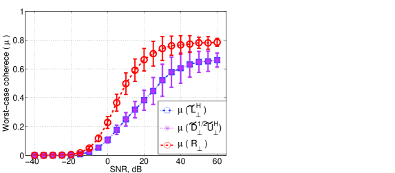
The covariance matrix $\boldsymbol{R}^{\perp}$ in (14) can be expressed compactly in terms of the SNR and CIR coefficients as $\boldsymbol{R}^{\perp}=\left[\boldsymbol{R}_{xx}^{-1}+\boldsymbol{H}^{H}\boldsymbol{R}_{nn}^{-1}\boldsymbol{H}\right]^{-1}=\left[\boldsymbol{I}+\mbox{SNR}\left(\boldsymbol{H}^{H}\boldsymbol{H}\right)\right]^{-1}$. This shows that, at low SNR, the noise dominates, i.e., $\boldsymbol{R}^{\perp}\approx\boldsymbol{I}$, and, consequently, $\mu\left(\boldsymbol{R}^{\perp}\right)\rightarrow 0$. As the SNR increases, the noise effect decreases and the CIR effect starts to appear, which makes $\mu\left(\boldsymbol{R}^{\perp}\right)$ converge to a constant. Typically, this constant, as shown through simulations, does not approach $1$.

On the other hand, $\boldsymbol{R}_{yy}$ has a well-structured (Hermitian Toeplitz) closed-form in terms of the CIR coefficients, filter time span $N_{f}$ and SNR, i.e., $\boldsymbol{R}_{yy}=\boldsymbol{H}\boldsymbol{H}^{H}+\mbox{$\frac{\mbox{1}}{SNR}$}\boldsymbol{I}$. Also, it is a square matrix with full rank, due to the presence of noise, and can be expressed in matrix form as

$$\boldsymbol{R}_{yy}=\mbox{Toeplitz}\overbrace{\left(\left[\begin{array}[]{ccccccc}r_{0}&r_{1}&\ldots&r_{v}&0&\ldots&0\end{array}\right]\right)}^{\boldsymbol{\phi}_{1}^{H}}\,,$$ (34)

where $r_{0}={\displaystyle\sum_{i=0}^{v}\left|h_{i}\right|^{2}+\left(\mbox{SNR}\right)^{-1}}$ and $r_{j}=\sum_{i=j}^{v}h_{i}h_{i-j}^{*},\,\forall j\neq 0$. In [28], we showed that the worst CIR vector $\boldsymbol{h}$, which is then used to estimate an upper-bound on $\mu(\boldsymbol{R}_{yy})$ for any given channel length $v$, can be derived by solving the following optimization problem

$$\widehat{\boldsymbol{h}}\triangleq\underset{\boldsymbol{h}}{\mbox{\mbox{arg}\mbox{max}}}\,\left|\boldsymbol{h}^{H}\boldsymbol{R}\boldsymbol{h}\right|\,\,\,\mbox{subject to}\,\,\,\boldsymbol{h}^{H}\boldsymbol{h}=1\,,$$ (35)

where $\boldsymbol{h}=\left[\begin{array}[]{cccc}h_{0}&h_{1}&\ldots&h_{v}\end{array}\right]^{H}$ is the length-$(v+1)$ CIR vector and $\boldsymbol{R}$ is a matrix that has ones along the super and sub-diagonals. It is known that the solution of (35) is the eigenvector corresponding to the maximum eigenvalue of $\boldsymbol{R}$. The eigenvalues $\lambda_{s}$ and eigenvectors $h_{j}^{(s)}$ of the matrix $\boldsymbol{R}$ have the following simple closed-forms [29]

$$\lambda_{s} = 2\,\mbox{cos}\left(\frac{\pi s}{v+2}\right)\,,\,h_{j}^{(s)}=\sqrt{\frac{2}{v+2}}\mbox{sin$\left(\frac{j\pi s}{v+2}\right),$}$$ (36)

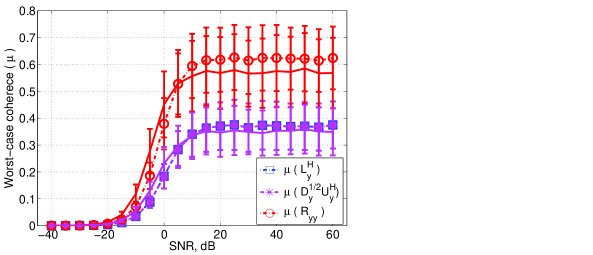
where $s,j=1,\ldots,v+1.$ By numerically evaluating $h_{j}^{(s)}$ for the maximum $\left|\lambda_{s}\right|$, we find that the worst-case coherence of $\boldsymbol{R}_{yy}$ (for any $v$) is sufficiently less than $1$. This observation points to the likely success of OMP in providing the sparsest solution $\widehat{\boldsymbol{z}}_{s}$ which corresponds to the dictionary that has the smallest $\mu(\boldsymbol{R}_{yy})$. Next, we propose a novel approach to perform the involved matrix factorizations in a reduced-complexity fashion.

IV-B Reduced-Complexity Design

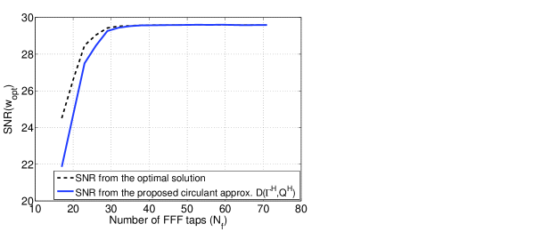
In this section, we propose reduced-complexity designs for the FIR filters discussed above, including LEs and DFEs, for MIMO systems. The proposed designs in Section III involve Cholesky factorization and/or eigen decomposition, whose computational costs could be large for channels with large delay spreads. For a Toeplitz matrix, the most efficient algorithms for Cholesky factorization are Levinson or Schur algorithms [30], which involve $\mathcal{O}(M^{2})$ computations, where $M$ is the matrix dimension. In contrast, since a circulant matrix is asymptotically equivalent to a Toeplitz matrix for reasonably large dimension [31], the eigen decomposition of a circulant matrix can be computed efficiently using the fast Fourier transform (FFT) and its inverse with only $\mathcal{O}\left(M\mbox{log}_{2}(M)\right)$ operations. We can use this asymptotic equivalence between Toeplitz and circulant matrices to carry out the computations needed for $\boldsymbol{R}_{yy},$ and $\boldsymbol{R}^{\perp}$ factorizations efficiently using the FFT and inverse FFT. In addition, direct matrix inversion can be avoided when computing the coefficients of the filters. This approximation turns out to be quite accurate from simulations as will be shown later.

It is well known that a circulant matrix, $\boldsymbol{C}$, has the discrete Fourier transform (DFT) basis vectors as its eigenvectors and the DFT of its first column as its eigenvalues. Thus, an $M\times M$ circulant matrix $\boldsymbol{C}$ can be decomposed as $\boldsymbol{C}$ =$\frac{1}{M}\boldsymbol{F}_{M}^{H}\boldsymbol{\varLambda}_{\boldsymbol{c}}\boldsymbol{F}_{M}$, where $\boldsymbol{F}_{M}$ is the DFT matrix with $f_{k,l}=e^{-j2\pi kl/M}$, $0\leq k,\,l\leq M-1$, and $\boldsymbol{\varLambda}_{\boldsymbol{c}}$ is an $M\times M$ diagonal matrix whose diagonal elements are the $M$-point DFT of $\boldsymbol{c}=\left\{c\right\}_{i=0}^{i=M-1}$, the first column of the circulant matrix. Further, from the orthogonality of DFT basis functions, $\boldsymbol{F}_{M}^{H}\boldsymbol{F}_{M}=\boldsymbol{F}_{M}\boldsymbol{F}_{M}^{H}=M\,\boldsymbol{I}_{M}$ and $\boldsymbol{F}_{N}^{H}\boldsymbol{F}_{N}=M\,\boldsymbol{I}_{N+1}$ where $\boldsymbol{F}_{N}$ is an $M\times N$ matrix, but $\boldsymbol{F}_{N}\boldsymbol{F}_{N}^{H}\neq M\,\boldsymbol{I}_{N+1}$ and instead $\boldsymbol{F}_{N}\boldsymbol{F}_{N}^{H}=N\left[\begin{array}[]{ccc}\boldsymbol{I}_{N}&\ldots&\boldsymbol{I}_{N}\end{array}\right]^{T}\left[\begin{array}[]{ccc}\boldsymbol{I}_{N}&\ldots&\boldsymbol{I}_{N}\end{array}\right]$.

We denote by $\overline{\boldsymbol{R}}_{yy},\,\overline{\boldsymbol{R}}_{yx}$, and $\overline{\boldsymbol{R}}^{\perp}$ the circulant approximations to the matrices $\boldsymbol{R}_{yy},\,\boldsymbol{R}_{yx}\mbox{,}$ $\mbox{ and }\boldsymbol{R}^{\perp}$ respectively. In addition, we denote the noiseless channel output vector as $\widetilde{\boldsymbol{y}},$ i.e., $\widetilde{\boldsymbol{y}}=\boldsymbol{Hx}$. We first derive the circulant approximation for the block Toeplitz matrix $\boldsymbol{R}_{yy}$ when $n_{o}\geq 2$, and the case of SISO systems follows as a special case of the block Toeplitz case by setting $n_{o}=n_{i}=1$.

The autocorrelation matrix $\boldsymbol{\overline{R}}_{yy}$ is computed as

$$\boldsymbol{\overline{R}}_{yy}=\underbrace{E\left[\widetilde{\boldsymbol{y}}_{k}\widetilde{\boldsymbol{y}}_{k}\right]}_{\overline{\boldsymbol{R}}_{\widetilde{y}\widetilde{y}}}+\underbrace{\frac{1}{SNR}}_{\sigma_{n}^{2}}\boldsymbol{I}_{N_{f}}.$$ (37)

To approximate the block Toeplitz $\boldsymbol{R}_{yy}$ as a circulant matrix, we assume that $\left\{\widetilde{\boldsymbol{y}}_{k}\right\}$ is cyclic. Hence, $E\left[\widetilde{\boldsymbol{y}}_{k}\widetilde{\boldsymbol{y}}_{k}\right]$ can be approximated as a time-averaged autocorrelation function as follows (defining $L=n_{o}N_{f}$)

$$\!\!\!\!\!\overline{\boldsymbol{R}}_{\widetilde{y}\widetilde{y}} \!\!\!\!= \!\!\!\frac{1}{N_{f}}\sum_{k=0}^{N_{f}-1}\widetilde{\boldsymbol{y}}_{k}\widetilde{\boldsymbol{y}}_{k}^{H}=\frac{1}{N_{f}}\boldsymbol{C}_{\underline{Y}}\boldsymbol{C}_{\underline{Y}}^{H}$$ (42)

$$\!\!\!\!= \!\!\!\frac{1}{N_{f}}\left(\frac{1}{L}\boldsymbol{F}_{L}^{H}\boldsymbol{\varLambda}_{\underline{\widetilde{Y}}}\boldsymbol{F}_{N_{f}}\right)\left(\frac{1}{L}\boldsymbol{F}_{N_{f}}^{H}\boldsymbol{\varLambda}_{\underline{\widetilde{Y}}}^{H}\boldsymbol{F}_{L}\right)$$

$$= \!\!\!\frac{1}{L^{2}}\boldsymbol{F}_{L}^{H}\boldsymbol{\varLambda}_{\widetilde{\underline{Y}}}\left[\begin{array}[]{c}\boldsymbol{I}_{N_{f}}\\ \vdots\\ \boldsymbol{I}_{N_{f}}\end{array}\right]\underbrace{\left[\begin{array}[]{ccc}\boldsymbol{I}_{N_{f}}&\ldots&\boldsymbol{I}_{N_{f}}\end{array}\right]}_{n_{o}\,\mbox{blocks}}\boldsymbol{\varLambda}_{\underline{\widetilde{Y}}^{H}}\boldsymbol{F}_{L}$$

$$= \!\!\!\frac{1}{L^{2}}\boldsymbol{F}_{L}^{H}\!\left[\!\!\begin{array}[]{c}\boldsymbol{\varLambda}_{\underline{\widetilde{Y}}^{1}}\\ \vdots\\ \boldsymbol{\varLambda}_{\widetilde{\underline{Y}}^{n_{o}}}\end{array}\!\!\right]\!\left[\!\!\begin{array}[]{ccc}\boldsymbol{\varLambda}_{\widetilde{\underline{Y}}^{1}}^{H}&\ldots&\boldsymbol{\varLambda}_{\widetilde{\underline{Y}}^{n_{o}}}^{H}\end{array}\!\!\right]\boldsymbol{F}_{L}\,,$$ (47)

where $\boldsymbol{F}_{L}$ is a DFT matrix of size $L\times L$, $\boldsymbol{F}_{N_{f}}$ is a DFT matrix of size $L\times N_{f}$, the column vector $\widetilde{\boldsymbol{\underline{Y}}}$ is the $L$-point DFT of $\widetilde{\boldsymbol{y}}_{1}=\left[\begin{array}[]{ccc}\widetilde{\boldsymbol{y}}_{N_{f}-1}^{T}&\widetilde{\boldsymbol{y}}_{N_{f}-2}^{T}\ldots&\widetilde{\boldsymbol{y}}_{0}^{T}\end{array}\right]$, $\widetilde{\boldsymbol{\underline{Y}}}^{i}$ is the $i^{th}$ subvector of $\widetilde{\boldsymbol{\underline{Y}}}$, i.e., $\widetilde{\underline{\boldsymbol{Y}}}$=$\left[\begin{array}[]{cccc}\widetilde{\boldsymbol{\underline{Y}}}^{1}&\widetilde{\boldsymbol{\underline{Y}}}^{2}&\ldots&\widetilde{\boldsymbol{\underline{Y}}}^{n_{o}}\end{array}\right]^{T}$, $\widetilde{\boldsymbol{y}}_{i}$ is the $n_{o}\times 1$ output vector and $\boldsymbol{C}_{y}=\mbox{{circ}($\widetilde{\boldsymbol{y}}_{1}$)}$ where circ denotes a circulant matrix whose first column is $\widetilde{\boldsymbol{y}}_{1}.$ Then,

$$\!\!\boldsymbol{\overline{R}}_{yy} \!\!\!\!=\!\!\!\! \overline{\boldsymbol{R}}_{\widetilde{y}\widetilde{y}}+n_{o}\sigma_{n}^{2}\boldsymbol{I}_{n_{o}N_{f}}$$ (52)

$$\!\!\!\!=\!\!\!\! \frac{1}{L^{2}}\boldsymbol{F}_{L}^{H}\!\left[\!\!\begin{array}[]{c}\boldsymbol{\varLambda}_{\widetilde{\underline{Y}}^{1}}\\ \vdots\\ \boldsymbol{\varLambda}_{\widetilde{\underline{Y}}^{n_{o}}}\end{array}\!\!\right]\underbrace{\!\!\left[\!\!\begin{array}[]{ccc}\boldsymbol{\varLambda}_{\widetilde{\underline{Y}}^{1}}^{H}&\ldots&\boldsymbol{\varLambda}_{\widetilde{\underline{Y}}^{n_{o}}}^{H}\end{array}\!\!\right]\!\!}_{\boldsymbol{\Psi}_{\underline{Y}}^{H}}\boldsymbol{F}_{L}+n_{o}\sigma_{n}^{2}\boldsymbol{I}_{L}$$

$$\!\!\!\!=\!\!\!\! \frac{1}{L^{2}}\boldsymbol{F}_{L}^{H}\left(\boldsymbol{\Psi}_{\underline{Y}}\boldsymbol{\Psi}_{\underline{Y}}^{H}+n_{o}L\sigma_{n}^{2}\boldsymbol{I}_{L}\right)\boldsymbol{F}_{L}=\boldsymbol{\varSigma\varSigma}^{H}.$$ (53)

Using the matrix inversion lemma [20], the inverse of $\boldsymbol{\overline{R}}_{yy}$ is

$$\!\!\boldsymbol{\overline{R}}_{yy}^{-1} \!\!\!=\!\!\! \left\{\frac{1}{L^{2}}\boldsymbol{F}_{L}^{H}\left(\boldsymbol{\Psi}_{\underline{Y}}\boldsymbol{\Psi}_{\underline{Y}}^{H}+n_{o}L\sigma_{n}^{2}\boldsymbol{I}_{L}\right)\boldsymbol{F}_{L}\right\}^{-1}$$ (54)

$$\!\!\!=\!\!\! \boldsymbol{F}_{L}^{H}\left(\boldsymbol{\Psi}_{\underline{Y}}\boldsymbol{\Psi}_{\underline{Y}}^{H}+n_{o}L\sigma_{n}^{2}\boldsymbol{I}_{L}\right)^{-1}\boldsymbol{F}_{L}$$

$$\!\!\!=\!\!\! \frac{1}{n_{o}L\sigma_{n}^{2}}\boldsymbol{F}_{L}^{H}\left(\boldsymbol{I}_{L}-\boldsymbol{\Psi}_{\underline{Y}}\boldsymbol{\varLambda}_{\varrho}^{-1}\boldsymbol{\Psi}_{\underline{Y}}^{H}\right)\boldsymbol{F}_{L}.$$

where $\varrho=\underbrace{\sum_{i=1}^{n_{o}}\left|\left\|\widetilde{\boldsymbol{\underline{Y}}}^{i}\right\|\right|^{2}}_{\overline{\varrho}}+n_{o}L\sigma_{n}^{2}\boldsymbol{1}_{L}$. Here, $\left|\left\|.\vphantom{\widetilde{\boldsymbol{\underline{Y}}}}\right\|\right|^{2}$ is defined as the element-wise norm square

$$\left|\left\|\left[\begin{array}[]{ccc}a_{0}&\!\!\ldots&\!a_{N_{f}-1}\end{array}\right]^{H}\right\|\right|^{2}\!\!=\!\!\left[\!\!\begin{array}[]{ccc}\left|a_{0}\right|^{2}\!\!&\!\ldots&\!\!\left|a_{N_{f}-1}\right|^{2}\end{array}\!\!\right]^{H}.$$ (55)

Notice that $\boldsymbol{\Psi}_{\underline{Y}}\boldsymbol{\Psi}_{\underline{Y}}^{H}=\sum_{i=1}^{n_{o}}\left|\left\|\boldsymbol{\widetilde{\underline{Y}}}^{i}\right\|\right|^{2}=N_{f}\sum_{i=1}^{n_{o}}\left|\left\|\boldsymbol{\underline{H}}^{i}\right\|\right|^{2}.$ Without loss of generality, we can write the noiseless channel output sequence $\widetilde{\boldsymbol{y}}_{k}$ in the discrete frequency domain as a column vector as follows

$$\widetilde{\boldsymbol{\underline{Y}}} = \boldsymbol{\underline{H}}^{H}\odot\underline{\boldsymbol{P}}_{\Delta}\odot\widetilde{\boldsymbol{\underline{X}}}$$ (56)

where $\odot$ denotes element-wise multiplication, $\widetilde{\boldsymbol{\underline{X}}}=\left[\begin{array}[]{ccc}\boldsymbol{\underline{X}}^{T}&\ldots&\boldsymbol{\underline{X}}^{T}\end{array}\right]^{T}$ where $\boldsymbol{\underline{X}}$ is the DFT of the data vector, $\boldsymbol{\underline{P}}_{\Delta}=\left[\begin{array}[]{ccc}\widetilde{\boldsymbol{\underline{P}}}_{\Delta}^{T}&\ldots&\widetilde{\boldsymbol{\underline{P}}}_{\Delta}^{T}\end{array}\right]^{T}$, $\widetilde{\boldsymbol{\underline{P}}}_{\Delta}=\left[\begin{array}[]{cccc}1&e^{-j2\pi\Delta/N_{f}}&\ldots&e^{-j2\pi\left(N_{f}-1\right)\Delta/N_{f}}\end{array}\right]^{T}$, and $\boldsymbol{\underline{H}}$ is the DFT of the CIRs, $\boldsymbol{\underline{H}}=\left[\begin{array}[]{ccc}\boldsymbol{\underline{H}}^{1T}&\ldots&\boldsymbol{\underline{H}}^{n_{o}T}\end{array}\right]^{T}$. To illustrate, for $n_{o}=1$, $\boldsymbol{\overline{R}}_{yy}$ in (53) reduces to

$$\boldsymbol{\overline{R}}_{yy} = \overline{\boldsymbol{R}}_{\widetilde{y}\widetilde{y}}+\sigma_{n}^{2}\boldsymbol{I}_{N_{f}}=\boldsymbol{F}_{N_{f}}^{H}(\boldsymbol{\varLambda}_{\varrho_{1}})\boldsymbol{F}_{N_{f}}=\boldsymbol{Q}\boldsymbol{Q}^{H}\,,$$ (57)

where $\varrho_{1}=N_{f}\left|\left\|\boldsymbol{\underline{H}}\right\|\right|^{2}+\sigma_{n}^{2}N_{f}\boldsymbol{1}_{N_{f}}$, $\boldsymbol{\underline{H}}$ is the $N_{f}$-point DFT of the CIR $\boldsymbol{h}$ and $\boldsymbol{\underline{P}}_{\Delta}=\widetilde{\boldsymbol{\underline{P}}}_{\Delta}$. Similarly, after some algebraic manipulations, $\overline{\boldsymbol{R}}^{\perp}$ can be expressed as

$$\overline{\boldsymbol{R}}^{\perp} = \frac{1}{L}\boldsymbol{F}_{N}^{H}\!\!\left(\!\!\boldsymbol{I}_{N}-\!\!\left[\!\!\begin{array}[]{c}\boldsymbol{I}_{M}\\ \vdots\\ \boldsymbol{I}_{M}\end{array}\right]\!\boldsymbol{\varLambda}_{\overline{\varrho}\varoslash\varrho}\!\left[\begin{array}[]{ccc}\boldsymbol{I}_{M}&\ldots&\boldsymbol{I}_{M}\end{array}\!\right]\!\!\right)\boldsymbol{F}_{N}$$ (62)

$$= \boldsymbol{\varTheta}\boldsymbol{\varTheta}^{H}\,,$$ (63)

where $\varoslash$ denotes element-wise division and $N=n_{i}(N_{f}+v)$. Notice that in the special case of SISO systems, i.e., $n_{i}=n_{o}=1$, $\overline{\boldsymbol{R}}^{\perp}$ can be expressed as follows

$$\overline{\boldsymbol{R}}^{\perp} = \boldsymbol{R}_{xx}-\boldsymbol{\overline{R}}_{yx}^{H}\boldsymbol{\overline{R}}_{yy}^{-1}\boldsymbol{\overline{R}}_{yx}$$ (64)

$$= \boldsymbol{I}_{N}-\boldsymbol{\overline{R}}_{xy}\left\{\frac{1}{N\sigma_{n}^{2}}\boldsymbol{F}_{N}^{H}\left(\boldsymbol{\varLambda}_{\widetilde{\underline{Y}}}\boldsymbol{\varLambda}_{\theta}^{-1}\boldsymbol{\varLambda}_{\widetilde{\underline{X}}}^{H}\right)\boldsymbol{F}_{N}\right\}$$

$$= \boldsymbol{I}_{N}-\left\{\frac{1}{N^{2}}\boldsymbol{F}_{N}^{H}\left(\boldsymbol{\varLambda}_{\underline{X}}\boldsymbol{\varLambda}_{\widetilde{\underline{Y}}}^{H}\boldsymbol{\varLambda}_{\widetilde{\underline{Y}}}\boldsymbol{\varLambda}_{\theta}^{-1}\boldsymbol{\varLambda}_{\underline{X}}^{H}\right)\boldsymbol{F}_{N}\right\}$$

$$= \frac{1}{N^{2}}\boldsymbol{F}_{N}^{H}\left(N\,\boldsymbol{I}_{N}-\boldsymbol{\varLambda}_{\underline{X}}\boldsymbol{\varLambda}_{\left(\overline{\theta}\varoslash\theta\right)}\boldsymbol{\varLambda}_{\underline{X}}^{H}\right)\boldsymbol{F}_{N}$$

$$= \frac{1}{N}\boldsymbol{F}_{N}^{H}\left(\boldsymbol{I}_{N}-\boldsymbol{\varLambda}_{\left(\overline{\theta}\varoslash\theta\right)}\right)\boldsymbol{F}_{N}=\boldsymbol{\varGamma}\boldsymbol{\varGamma}^{H},$$

where $N=N_{f}+v$, $\boldsymbol{F}_{N}$ is an $N\times N$ DFT matrix, $\boldsymbol{F}_{N_{f}}$ is an $N\times N_{f}$ DFT matrix, $\theta=\overline{\theta}+N\sigma_{n}^{2}\boldsymbol{1}_{N}$ and $\overline{\theta}=\left|\left\|\widetilde{\underline{\boldsymbol{Y}}}\right\|\right|^{2}$. Note that $\widetilde{\underline{\boldsymbol{Y}}}$ is the $N$-point DFT of $\left[\begin{array}[]{cccc}\widetilde{y}_{N_{f}}^{T}&\widetilde{y}_{N_{f}-1}^{T}&\ldots&\widetilde{y}_{1}^{T}\end{array}\right]$.

In summary, the proposed design method for the sparse FIR filters involves the following steps:

1. An estimate for the channel between the input(s) and the output(s) of the actual transmission channel is obtained. Then, the matrices defined in Table I are computed.

2. The required matrices involved in our design, i.e., $\boldsymbol{R}^{\perp}$or $\boldsymbol{R}_{yy}$, are factorized using reduced-complexity design discussed above in this section.

3. Based on a desired performance-complexity tradeoff, $\epsilon$ is computed. Afterward, the dictionary with the smallest coherence is selected for use in designing the sparse FIR filter.

4. The parameters $\boldsymbol{\varPhi}$, $\boldsymbol{d}$, and $\boldsymbol{K}$ are jointly used to estimate the locations and weights of the filter taps using the OMP algorithm.

We conclude this section by noting that using this low-complexity fast computation matrix factorization approach, we are able to design the FIR filters in a reduced-complexity manner where neither a Cholesky nor an eigen factorization is needed. Furthermore, direct inversion of the matrices involved in the design of filters is avoided.

IV-C Complexity Analysis

In this section, we evaluate the computation complexity of various filter designs in terms of complex multiplications/additions (CM/A). For the proposed sparse MIMO LEs and DFEs, the main computational tasks are factorizations of the matrices $\boldsymbol{R}_{yy}$, $\boldsymbol{R}^{\perp}$ and the OMP computations. It is noted in [23] that the computation cost, CM/A, of OMP is $\mathcal{O}\left(MNS\right)$, where $MN$ is the size of the equalizer vector/matrix and $S$ is the number of nonzero entries of $\boldsymbol{z}_{s}$. Note that an additional $\mathcal{O}\left(S^{3}\right)$ CM/A computations are required to obtain the restricted least squares estimate of $\boldsymbol{z}_{s}$ [26]. Hence, the total cost to estimate $\boldsymbol{z}_{s}$ using our proposed design method is the sum of the factiorization cost of the involved matrices in the FIR filter design, the OMP cost, and the restricted least squares cost, i.e., $\mathcal{O}\left(M\,\mbox{log}\left(M\right)+MNS+S^{3}\right)$, which is typically much lower than the computational complexity of $\mathcal{O}\left(M^{3}+NM^{2}\right)$ for convex-optimization-based approaches [26]. Furthermore, the cost of our proposed method is much smaller than the cost required to estimate the optimum FIR equalizers given in [10]. The complexity of our proposed design method as compared to the optimum equalizers and some other sparse designs from the literature is summarized in Table III. Next, we will report the results of our numerical experiments to evaluate the performance of our proposed framework considering different FIR filter designs and using different sparsifying dictionaries for each design.

Table III: Computational complexity of various equalizer designs.

Equalizer Type	Design Complexity
Optimum FIR LEs [10]	$\mathcal{O}\left(n_{i}\left(N_{f}+v\right)\left(n_{o}N_{f}\right)^{2}+n_{o}^{3}N_{f}^{2}\right)$
Optimum FIR DFEs [10]	FBF: $\mathcal{O}\left(n_{i}^{3}\left(N_{b}+1\right)^{3}+n_{i}^{3}+n_{i}^{3}\left(N_{b}+1\right)\right)$
	FFF: $\mathcal{O}\left(n_{i}\left(N_{f}+v\right)\left(n_{o}N_{f}\right)^{2}+n_{i}^{2}\left(N_{b}+1\right)^{2}\right)$
Sparse FIR LEs [15]	$\mathcal{O}\left(\left(n_{o}N_{f}\right)^{2}+n_{o}n_{i}N_{f}S+S^{3}\right)$
Sparse FIR DFEs [15]	FBF: $\mathcal{O}\left(\left(N_{f}+v\right)^{2}+n_{i}^{2}\left(N_{f}+v\right)^{2}S+S^{3}\right)$
	FFF: $\mathcal{O}\left(\left(n_{o}N_{f}\right)^{2}+\left(n_{o}N_{f}\right)^{2}S+S^{3}\right)$
Proposed Sparse FIR LEs	$\mathcal{O}\left(\left(n_{o}N_{f}\right)\mbox{log}\left(n_{o}N_{f}\right)+n_{o}n_{i}N_{f}S+S^{3}\right)$
Proposed Sparse FIR DFEs	FBF:$\mathcal{O}\left(\left(N_{f}+v\right)\mbox{log}\left(N_{f}+v\right)+n_{i}^{2}\left(N_{f}+v\right)^{2}S+S{}^{3}\right)$
	FFF: $\mathcal{O}\left(\left(n_{o}N_{f}\right)\mbox{log}\left(n_{o}N_{f}\right)+\left(n_{o}N_{f}\right)^{2}S+S^{3}\right)$

V Numerical Results

We now investigate the performance of our proposed framework. The CIRs used in our numerical results are unit-energy symbol-spaced FIR filters with $v$ taps generated as zero-mean unit-variance uncorrelated complex Gaussian random variables. The CIR taps are assumed to have a uniform power-delay-profile (UPDP). Note that this type of channel is rather difficult to equalize because its PDP is uniform and non-sparse. The performance results are calculated by averaging over 5000 channel realizations. Error bars, when used, show the confidence intervals of the data, i.e., the standard deviation along a curve. We use the notation $\boldsymbol{D}(\boldsymbol{\chi}_{f})$ to refer to a LE designed using the sparsifying dictionary $\boldsymbol{\chi}_{f}$, while $\boldsymbol{D}(\boldsymbol{\chi}_{b},\,\boldsymbol{\chi}_{f})$ is used to refer to a FBF designed using the sparsifying dictionary $\boldsymbol{\chi}_{b}$ and a FFF designed using the sparsifying dictionary $\boldsymbol{\chi}_{f}$. Note that [15] follows as a special case of our proposed design method by choosing the classical Cholesky (of the form $\boldsymbol{L}\boldsymbol{L}^{H}$) as the factorization method and keeping the parameter $\boldsymbol{K}$ in (28) always equal to the identity matrix, e.g., $\boldsymbol{K}=\boldsymbol{I}$, $\boldsymbol{\Phi}=\boldsymbol{L}^{H}$ and $\boldsymbol{d}$ = $\boldsymbol{L}_{y}^{-1}\boldsymbol{r}_{\Delta}$. Hence, in the results below, we have implicitly compared with the approach proposed in [15] when such setting is used.

To quantify the accuracy of approximating Toeplitz matrices, e.g., $\boldsymbol{R}_{yy}$ and $\boldsymbol{R}^{\perp}$, by their equivalent circulant matrices, e.g, $\boldsymbol{\overline{R}}_{yy}$ and $\overline{\boldsymbol{R}}^{\perp}$, respectively, we plot the optimal output SNR and the output SNR obtained from the circulant approximation versus the number of FFF taps ($N_{f}$) in Figure 1. The gap between the optimal output SNR and the output SNR from the circulant approximation approaches zero as the number of the FFF taps increases, as expected. A good rule of the thumb for $N_{f}$, to obtain an accurate approximation, would be $N_{f}\geq 4v$.

Figure 1: Performance of circulant approximation based approach for UPDP channel with $v=8$ and input $\mbox{SNR}=30\,\mbox{dB}$.

Figure 2: Worst-case coherence for sparsifying dictionaries $\widetilde{\boldsymbol{L}}_{\perp}$ and $\widetilde{\boldsymbol{D}}_{\perp}^{\frac{1}{2}}\widetilde{\boldsymbol{U}}_{\perp}^{H}$ versus input SNR for UPDP with $v=8$ and $N_{f}=80$. Note that we estimate $\mu\left(\widetilde{\boldsymbol{D}}_{\perp}^{\frac{1}{2}}\widetilde{\boldsymbol{U}}_{\perp}^{H}\right)$ and $\mu\left(\widetilde{\boldsymbol{L}}_{\perp}^{H}\right)$ after removing the $\left(\Delta+1\right)^{th}$ column as discussed in (23). Moreover, changing the $\left(\Delta+1\right)^{th}$ location has insignificant effect on $\mu(\boldsymbol{\varPhi})$ to show.

Figure 3: Worst-case coherence for the sparsifying dictionaries $\boldsymbol{L}_{y}^{H}$, $\boldsymbol{D}_{y}^{\frac{1}{2}}\boldsymbol{U}_{y}^{H}$ and $\boldsymbol{R}_{yy}$ versus input SNR for UPDP with $n_{i}=2,\,n_{o}=2$, $v=8$ and $N_{f}=80$. Solid lines represent the coherence of the corresponding circulant approximation for $\boldsymbol{D}_{y}^{\frac{1}{2}}\boldsymbol{U}_{y}^{H}$ (i.e., $\boldsymbol{\Sigma^{H}}$) and $\boldsymbol{R}_{yy}$ (i.e., $\boldsymbol{\overline{R}}_{yy}=$$\boldsymbol{\Sigma}\boldsymbol{\Sigma^{H}}$).

Figure 4: Percentage of active taps versus the performance loss ($\eta_{max}$) for the sparse MIMO-LEs with SNR (dB) $=10,\,30$,$\,n_{o}=2,\,n_{i}=2$, $v=8$ and $N_{f}=80$.

Figure 5: SER comparison between the non-sparse MMSE MIMO-LEs, the proposed sparse MIMO-LEs $\boldsymbol{D}(\boldsymbol{D}_{y}^{\frac{1}{2}}\boldsymbol{U}_{y}^{H})$, $\boldsymbol{D}(\boldsymbol{L}_{y}^{H})$, $\boldsymbol{D}(\boldsymbol{R}_{yy})$ and the “significant taps” based LE (proposed in [16]) with sparsity level = 35%, $n_{i}=2$, $n_{o}=2$, $v=5$ , $N_{f}=40$ and 16-QAM modulation.

Figure 6: Percentage of active FFF taps versus the performance loss ($\eta_{max}$) for sparse DFE designs with SNR = 20 dB, $v=8$ and $N_{f}=80$.

Figure 7: Maximum output SNR versus FFF taps for UPDP CIR with $v=8$, $N_{f}=80$ and SNR = $30$ dB. Solid lines represent the $\boldsymbol{D}(\boldsymbol{\varGamma}^{H},\boldsymbol{Q}^{H})$ approach, while the dashed lines represent the “significant taps” approach proposed in [16].

Figure 8: SER comparison between the MMSE non-sparse DFEs, i.e., $\boldsymbol{D}(\boldsymbol{\varTheta}^{H},\boldsymbol{\Sigma}^{H})$ with $\eta_{max}=0$, the proposed sparse DFEs $\boldsymbol{D}(\boldsymbol{L}_{y}^{H},\boldsymbol{L}_{y}^{H})$, $\boldsymbol{D}(\boldsymbol{\varTheta}^{H},\boldsymbol{\Sigma}^{H})$ and the $\boldsymbol{D}(\boldsymbol{\varTheta}^{H},\boldsymbol{R}_{yy})$ for SISO and MIMO systems with $n_{i}=2,\,n_{o}=2$, $v=8$, $N_{b}=8$, $N_{f}=80$, $\eta_{max}=0.25$ dB and 16-QAM modulation.

To investigate the coherence of the sparsifying dictionaries used in our analysis, we plot the worst-case coherence versus the input SNR in Figure 2 for sparsifying dictionaries $\widetilde{\boldsymbol{L}}_{\perp}$ and $\boldsymbol{D}_{\perp}^{{}^{\frac{1}{2}}}\widetilde{\boldsymbol{U}}_{\perp}^{H}$ (which is formed by all columns of $\boldsymbol{D}_{\perp}^{\frac{1}{2}}\boldsymbol{U}_{\perp}^{H}$ except the $\left(\Delta+1\right)^{th}$ column) generated from $\boldsymbol{R}_{\perp}$. Note that a smaller value of $\mu(\boldsymbol{\Phi})$ indicates that a sparser approximation is more likely. Both sparsifying dictionaries have the same $\mu\left(\boldsymbol{\varPhi}\right)$, which is strictly less than $1$. Similarly, in Figure 3, we plot the worst-case coherence of the proposed sparsifying dictionaries used to design sparse MIMO-LEs and MIMO-DFEs. At high SNR levels, the noise effects are negligible and, hence, the sparsifying dictionaries (e.g., $\boldsymbol{R}_{yy}\approx\boldsymbol{H}\boldsymbol{H}^{H}$) do not depend on the SNR. As a result, the coherence converges to a constant. On the other hand, at low SNR, the noise effects dominate the channel effects. Hence, the channel can be approximated as a memoryless (i.e., 1 tap) channel. Then, the dictionaries (e.g., $\boldsymbol{R}_{yy}\approx\frac{1}{SNR}\boldsymbol{I}$) can be approximated as a multiple of the identity matrix, i.e., $\mu\left(\boldsymbol{\varPhi}\right)\rightarrow 0$.

Next, we compare different sparse FIR LE and DFE designs based on different sparsifying dictionaries to study the effect of $\mu\left(\boldsymbol{\varPhi}\right)$ on their performance. The OMP algorithm is used to compute the sparse approximations. The OMP stopping criterion is set to be a predefined sparsity level (number of nonzero entries) or a function of the PRE such that: Performance Loss ($\eta$)$=10\,\mbox{Log}_{10}\left(\frac{SNR(\widehat{\boldsymbol{z}}_{s})}{SNR(\boldsymbol{z}_{opt})}\right)\leq 10\,\mbox{Log}_{10}\left(1+\frac{\epsilon}{\xi_{m}}\right)\triangleq\eta_{max}$. Here, $\epsilon$ is computed based on an acceptable $\eta_{max}$ and, then, the coefficients of $\widehat{\boldsymbol{z}}_{s}$ are computed through (28). The percentage of the active taps is calculated as the ratio between the number of nonzero taps to the total number of filter taps. For the MMSE equalizer, where none of the coefficients is typically zero, the number of active filter taps is equal to the filter span. The decision delay for LEs is set to be $\Delta\approx\frac{N_{f}+v}{2}$ [33], while for DFEs we set $\Delta\approx N_{f}-1$, which is optimum when $N_{b}=v$ [34].

Figure 4 plots the percentage of the active taps versus the performance loss $\eta_{max}$ for the proposed sparse FIR MIMO-LEs and the proposed approach in [16], which we refer to it as the “significant taps” approach. In that approach, all of the FIR filter taps are computed and only the $\nu$-significant ones are retained. We observe that a lower active taps percentage is obtained when the coherence of the sparsifying dictionary is small. For instance, allowing for $0.25$ dB SNR loss results in a significant reduction in the number of active LE taps. Approximately two-thirds (respectively, two-fifths) of the taps are eliminated when using $\boldsymbol{D}_{y}^{\frac{1}{2}}\boldsymbol{U}_{y}^{H}$ and $\boldsymbol{L}_{y}^{H}$ at SNR equal to 10 (respectively, 30). The sparse MIMO-LE designed based on $\boldsymbol{R}_{yy}$ needs more active taps to maintain the same SNR loss as that of the other sparse MIMO-LEs due to its higher coherence. This suggests that the smaller the worst-case coherence of the dictionary in our setup, the sparser is the equalizer. Moreover, a lower sparsity level (active taps percentage) is achieved at higher SNR levels, which is consistent with the previous findings (e.g., in [35]). Furthermore, reducing the number of active taps decreases the filter equalization design complexity and, consequently, power consumption since a smaller number of complex multiply-and-add operations are required.

In Figure 5, we compare the symbol error rate (SER) performance of our proposed sparse FIR MIMO-LEs with the “significant taps” approached proposed in [5]. Assuming a $25\%$ sparsity level, both the $\boldsymbol{D}(\boldsymbol{D}_{y}^{\frac{1}{2}}\boldsymbol{U}_{y}^{H})$ and $\boldsymbol{D}(\boldsymbol{L}_{y}^{H})$ sparse LEs achieve the lowest SER followed by $\boldsymbol{D}(\boldsymbol{R}_{yy})$, while the “significant taps” performs the worst. In addition to this performance gain, the complexity of the proposed sparse LEs is less than that of the “significant-taps” LE since only an inversion of an $N_{s}\times N_{s}$ matrix is required (not $N_{f}\times N_{f}$ as in the “significant-taps” approach) where $N_{s}$ is the number of nonzero taps. Although the $\boldsymbol{D}(\boldsymbol{D}_{y}^{\frac{1}{2}}\boldsymbol{U}_{y}^{H})$ and $\boldsymbol{D}(\boldsymbol{L}_{y}^{H})$ LEs achieve almost the same SER, the former has a lower decomposition complexity since its computation can be done efficiently using only the FFT and its inverse.

The effect of our sparse FFF and FBF FIR filter designs for SISO DFEs on the performance is shown in Figure 6. We plot the active (non-zero) FFF taps percentage of the total FFF span $N_{f}$ versus the maximum loss in the output SNR. Allowing a higher loss in the output SNR yields a bigger reduction in the number of active FFF taps. Moreover, the active FFF taps percentage increases as $N_{b}$ decreases because the equalizer needs more taps to equalize the CIR. We also observe that allowing a maximum of only $0.25$ dB in SNR loss with $N_{b}=4$ results in a substantial $60\%$ reduction in the number of FFF active taps (the equalizer can equalize the channel using only 32 out of 80 taps).

In Figure 7, we compare our proposed sparse FBF design with that in [16], i.e., the “significant taps” approach, in terms of output SNR where we plot the output SNR versus FFF taps $N_{f}$ for the UPDP channel. We vary $N_{b}$, the number of FBF taps, from $1$ (lower curve) to $10$ (upper curve). The output SNR increases as $N_{b}$ increases for all FBF designs, as expected, and our sparse FBF outperforms, for all scenarios, the proposed approach in [16]. Notice that as $N_{b}$ increases, the sparse FBF becomes more efficient in removing ISI from previously-detected symbols resulting in a higher SNR.

In Figure 8, we study the SER performance of our proposed sparse SISO-DFEs and MIMO-DFEs versus the input SNR based on different design criteria and using different sparsifying dictionaries. Assuming a maximum SNR loss of $0.25$ dB, both $\boldsymbol{D}(\boldsymbol{L}_{y}^{H},\boldsymbol{L}_{y}^{H})$ and $\boldsymbol{D}(\boldsymbol{\varTheta}^{H},\boldsymbol{\Sigma}^{H})$ sparse SISO/MIMO DFEs designs achieve the lowest SER, followed by $\boldsymbol{D}(\boldsymbol{\varTheta}^{H},\boldsymbol{R}_{yy})$. Note that $\eta_{max}=0$ corresponds to the optimum non-sparse MMSE design where all the equalizer taps are active. Additionally, at high SNR, diversity gains of the MIMO-DFEs over the SISO-DFEs are noticed resulting in a better performance.

VI Conclusions

In this paper, we proposed a general framework for designing sparse FIR MIMO LEs and DFEs based on a sparse approximation formulation using different dictionaries. Based on the asymptotic equivalence of Toeplitz and circulant matrices, we also proposed reduced-complexity designs, for all proposed FIR filters, where matrix factorizations can be carried out efficiently using the FFT and inverse FFT with negligible performance loss as the number of filter taps increases. In addition, we analyzed the coherence of the proposed dictionaries involved in our design and showed that the dictionary with the smallest coherence gives the sparsest filter design. Finally, the significance of our approach was shown analytically and quantified through simulations.

References

• [1] Y. Wu, M. Zhu, and X. Li, “Sparse linear equalizers for turbo equalizations in underwater acoustic communication,” in OCEANS 2015 - MTS/IEEE Washington, Oct 2015, pp. 1–6.
• [2] F. C. Ribeiro, E. C. Marques, N. M. Paiva, and J. F. Galdino, “Sparsity-Aware direct decision-feedback equalization of ionospheric HF channels,” in IEEE Military Communications Conference, MILCOM, 2015, pp. 1467–1472.
• [3] D. Wei, C. Sestok, and A. Oppenheim, “Sparse filter design under a quadratic constraint: Low-complexity algorithms,” IEEE Trans. on Sig. Processing, vol. 61, no. 4, pp. 857–870, 2013.
• [4] D. Wei and A. Oppenheim, “A branch-and-bound algorithm for quadratically-constrained sparse filter design,” IEEE Trans. on Sig. Processing, vol. 61, no. 4, pp. 1006–1018, 2013.
• [5] M. Melvasalo, P. Janis, and V. Koivunen, “Sparse equalization in high data rate WCDMA systems,” in IEEE 8th SPAWC, 2007, pp. 1–5.
• [6] T. Baran, D. Wei, and A. Oppenheim, “Linear programming algorithms for sparse filter design,” IEEE Trans. on Sig. Processing, vol. 58, no. 3, pp. 1605–1617, 2010.
• [7] G. Kutz and A. Chass, “Sparse chip equalizer for DS-CDMA downlink receivers,” IEEE Commun. Letters, vol. 9, no. 1, pp. 10–12, 2005.
• [8] S. Ariyavisitakul, N. R. Sollenberger, and L. J. Greenstein, “Tap-selectable decision feedback equalization,” in Communications, 1997. ICC’97 Montreal, Towards the Knowledge Millennium. 1997 IEEE International Conference on, vol. 3.   IEEE, 1997, pp. 1521–1526.
• [9] N. Al-Dhahir and C. Fragouli, “How to choose the number of taps in a DFE?” in IEEE Annual Conference on Information Sciences and Systems (CISS 2002), no. ARNI-CONF-2007-011, 2002.
• [10] N. Al-Dhahir and A. Sayed, “The finite-length multi-input multi-output MMSE-DFE,” IEEE Trans. on Sig. Processing, vol. 48, no. 10, pp. 2921–2936, Oct 2000.
• [11] “Guidelines for The Evaluation of Radio Transmission Technologies for IMT-2000 [Available online]: .” Recommendation ITU-R M.1225, 1997.
• [12] IEEE-P802.15, “TG3C Channel Modeling Sub-committee Final Report,” 2009.
• [13] F. K. Lee and P. J. McLane, “Design of nonuniformly spaced tapped-delay-line equalizers for sparse multipath channels,” IEEE Trans. on Commun., vol. 52, no. 4, pp. 530–535, 2004.
• [14] E. Vlachos, A. S. Lalos, and K. Berberidis, “Stochastic gradient pursuit for adaptive equalization of sparse multipath channels,” IEEE Journal on Emerging and Selected Topics in Circuits and Systems, vol. 2, no. 3, pp. 413–423, 2012.
• [15] A. Gomaa and N. Al-Dhahir, “A new design framework for sparse FIR MIMO equalizers,” IEEE Trans. on Commun., vol. 59, no. 8, pp. 2132–2140, 2011.
• [16] S. Roy, T. M. Duman, and V. K. McDonald, “Error rate improvement in underwater MIMO communications using sparse partial response equalization,” IEEE Journal of Oceanic Engineering, vol. 34, no. 2, pp. 181–201, 2009.
• [17] J. Proakis and M. Salehi, Digital Communications, 5th Edition.   New York, NY, USA: McGraw-Hill, 2007.
• [18] N. Al-Dhahir, “FIR channel-shortening equalizers for MIMO ISI channels,” IEEE Trans. on Commun., vol. 49, no. 2, pp. 213–218, 2001.
• [19] A. O. Al-Abbasi, R. Hamila, W. U. Bajwa, and N. Al-Dhahir, “Sparsifying dictionary analysis for fir mimo channel-shortening equalizers,” in 2016 IEEE 17th International Workshop on Signal Processing Advances in Wireless Communications (SPAWC), 2016, pp. 1–6.
• [20] R. A. Horn and C. R. Johnson, Eds., Matrix Analysis.   New York, NY, USA: Cambridge University Press, 1986.
• [21] C. Xing, F. Gao, and Y. Zhou, “A framework for transceiver designs for multi-hop communications with covariance shaping constraints,” IEEE Transactions on Signal Processing, vol. 63, no. 15, Aug 2015.
• [22] A. O. Al-Abbasi, R. Hamila, W. U. Bajwa, and N. Al-Dhahir, “Design and Analysis Framework for Sparse FIR Channel Shortening.”   IEEE ICC’16 Conference, 2016, pp. 1–7.
• [23] J. Tropp and A. Gilbert, “Signal recovery from random measurements via orthogonal matching pursuit,” IEEE Trans. on Info. Theory, vol. 53, no. 12, pp. 4655–4666, 2007.
• [24] D. L. Donoho, “Compressed sensing,” IEEE Trans. on Info. Theory, vol. 52, no. 4, pp. 1289–1306, 2006.
• [25] X. Feng et al., “Sparse equalizer filter design for multi-path channels,” Master’s thesis, Massachusetts Institute of Technology, 2012.
• [26] W. U. Bajwa and A. Pezeshki, “Finite frames for sparse signal processing,” in Finite Frames.   Springer, 2013.
• [27] J. Tropp, “Greed is good: algorithmic results for sparse approximation,” IEEE Trans. on Info. Theory,, vol. 50, no. 10, pp. 2231–2242, 2004.
• [28] A. O. Al-Abbasi, R. Hamila, W. U. Bajwa, and N. Al-Dhahir, “A General Framework for the Design and Analysis of Sparse FIR Linear Equalizers.”   IEEE GlobalSIP Conference, 2015, pp. 1–5.
• [29] G. H. Golub, “CME 302: Eigenvalues of Tridiagonal Toeplitz Matrices,” Stanford University, USA.
• [30] M. H. Hayes, Statistical Digital Signal Processing and Modeling, 1st ed.   New York, NY, USA: John Wiley & Sons, Inc., 1996.
• [31] J. Pearl, “On coding and filtering stationary signals by discrete Fourier transforms (Corresp.),” IEEE Trans. on Info. Theory, vol. 19, no. 2, pp. 229–232, 1973.
• [32] R. M. Gray, “On the asymptotic eigenvalue distribution of Toeplitz matrices,” IEEE Trans. on Info. Theory, vol. 18, no. 6, pp. 725–730, 1972.
• [33] J. Cioffi, “EE379A notes Chapter 3,” Stanford University, USA.
• [34] N. Al-Dhahir and J. Cioffi, “MMSE decision-feedback equalizers: finite-length results,” IEEE Trans. on Info Theory, vol. 41, no. 4, pp. 961–975, Jul 1995.
• [35] G. Kutz and D. Raphaeli, “Determination of tap positions for sparse equalizers,” IEEE Trans. on Commun., vol. 55, no. 9, pp. 1712–1724, 2007.