Choosing the number of groups in a latent stochastic block model for dynamic networks

Abstract

Latent stochastic block models are flexible statistical models that are widely used in social network analysis. In recent years, efforts have been made to extend these models to temporal dynamic networks, whereby the connections between nodes are observed at a number of different times. In this paper we extend the original stochastic block model by using a Markovian property to describe the evolution of nodes’ cluster memberships over time. We recast the problem of clustering the nodes of the network into a model-based context, and show that the integrated completed likelihood can be evaluated analytically for a number of likelihood models. Then, we propose a scalable greedy algorithm to maximise this quantity, thereby estimating both the optimal partition and the ideal number of groups in a single inferential framework. Finally we propose applications of our methodology to both real and artificial datasets.

Keywords: Stochastic Block Models, Dynamic Networks, Greedy Optimisation, Bayesian Inference, Integrated Completed Likelihood.

1 Introduction

In the last few years, there has been an increasing amount of data stored characterising interactions between individuals or, more generally, units of interest. An interaction, represented by a triple $(i,j,\eta)$, indicates that units $i$ and $j$ have a connection at a specific time point $\eta$. Interactions can for instance describe email exchanges between individuals or posts on social media. In Biology, units can correspond to genes and interactions to regulation events between the genes. A natural approach to model the set of all observed interactions is to rely on a dynamic graph where each unit is associated with a node and an edge $(i,j)$ is present between two units $i$ and $j$, at time $\eta$, if the interaction $(i,j,\eta)$ is recorded.

A long series of methods have been proposed recently to cluster the nodes of dynamic networks in order to summarise the information hidden in such data. A large number of these consider the Stochastic Block Model (SBM) [22, 17] as a starting point and propose extensions to the dynamic framework. Moreover, they are usually discrete in time, that is, predefined time intervals are introduced and interactions during those time intervals are aggregated to obtain snapshots indexed by a discrete time variable $t$. In the case of a binary dynamic network, two nodes are connected in a snapshot if they have at least one interaction in the corresponding time interval. We recall that the SBM was originally introduced to cluster nodes in static networks where nodes and edges do not evolve through time. The model assumes that nodes are spread in latent clusters, which, in practice, have to be inferred from the data. The probability for two nodes to connect is then only dependent on their respective clusters. Because no constraints are imposed on the connection probabilities, various types of clusters can be extracted from the data, which makes methodologies based on SBM applicable to networks with different connectivity structures [7]. The dynamic SBM-like model of [26] allows, for example, each node to switch its cluster at time $t$ depending on its state at time $t-1$. A transition matrix is employed to characterise the switching probabilities. While clusters can change over time, fixed connection probabilities are used. Conversely, the model of [25] relies on evolving connection probabilities and temporal changes are described through a state space model. Therefore, the inference requires the use of optimisation tools such as the Kalman filter and the Rauch-Tung-Striebel smoother. The work of [26] was then extended by [13] for the clustering of nodes in dynamic networks where edges are not necessarily binary. We emphasise that theoretical results are also provided in their paper to show that dynamic SBM-like models should not let both the clusters and connection parameters evolve through time without incurring into identifiability issues.

In the static framework, many extensions have been considered for the SBM model. Many of them have then been adapted to deal with dynamic networks. For example, the well-known mixed-membership SBM of [1] has been extended to a dynamic framework by several works including [24], [10] and [12]. Note that the latent position model of [11], which is also popular in the network community, was also adapted by [19] and [8] to deal with dynamic interactions.

In this paper, our objective is to model the evolution of the cluster memberships over time by relying on a Markovian property. We take advantage of prior conjugacy to integrate out analytically most of the model parameters, with an approach similar to that of [15] and [5]. This so-called collapsing allows one to obtain an analytical expression for the integrated completed data likelihood for a number of likelihood models. A greedy optimisation algorithm is then employed for inferential purposes. It allows estimation of both the number of clusters and the cluster memberships of the nodes to the clusters.

Section 2 introduces the model and the notation. A Bayesian hierarchical structure is then proposed in Section 3. Finally, the optimisation procedure is given in Section 5 and experiments are carried out in Sections 6, 7, and 8 to assess the proposed methodology.

2 Markovian Stochastic Block Model

The observed data consist of a sequence of network objects $\mathcal{X}=\left\{\textbf{X}^{(t)}\right\}_{t\in\mathcal{T}}$ defined on the same set of nodes $\mathcal{V}=\left\{1,\dots,N\right\}$. We focus our attention on dynamic networks, where $\mathcal{T}=\left\{1,\dots,T\right\}$ denotes the temporal span.

The random variable $X_{ij}^{(t)}$ models the value exhibited by the edge from $i$ to $j$ at time $t$, $\forall t\in\mathcal{T}$ and $\forall i,\ j\in\mathcal{V}$. We outline our methodology on directed networks, however it applies also to undirected network as we illustrate in the applications we consider. A typical scenario is that of a binary dynamic network, where:

$$x_{ij}^{(t)}=\begin{cases}1,&\mbox{ if an edge from $i$ to $j$ appears at time $t$; }\\ 0,&\mbox{ otherwise. }\end{cases}$$ (1)

Also, self-edges are not allowed, i.e. $x_{ii}^{(t)}=0,\ \forall t\in\mathcal{T}$ and $\forall i\in\mathcal{V}$.

The random variable $Z_{i}^{(t)}$ characterises the allocation of a node, whereby $Z_{i}^{(t)}=g$ indicates that node $i$ is allocated to group $g$ at time $t$, for a certain $g\in\mathcal{K}=\left\{1,\dots,K\right\}$. The set $\textbf{Z}^{(t)}=\left\{Z_{i}^{(t)}\right\}_{i\in\mathcal{V}}$ therefore corresponds to a random hard clustering (i.e. a partitioning) of $\mathcal{V}$, $\forall t\in\mathcal{T}$. We also denote the full set of allocations with $\mathcal{Z}=\left\{\textbf{Z}^{(t)}\right\}_{t\in\mathcal{T}}$. The total number of groups in this underlying structure is denoted by $K$, hence $Z_{i}^{(t)}\in\mathcal{K},\ \forall t\in\mathcal{T}$ and $\forall i\in\mathcal{V}$. Note that $K$ represents the total number of groups in $\mathcal{Z}$, implying that, at each time frame $t$, the current number of non-empty groups $K^{(t)}$ may be any number in $\mathcal{K}$.

The allocations characterise the connection profiles of the nodes of the network, in that nodes allocated to the same group have their edges drawn from the same probability distribution. The edges of the dynamic network are marginally dependent, however they are conditionally independent given the allocations:

$$p\left(\mathcal{X}\middle|\mathcal{Z}\right)=\prod_{t\in\mathcal{T}}p\left(\textbf{X}^{(t)}\middle|\textbf{Z}^{(t)}\right),$$ (2)

and $\forall t\in\mathcal{T}$:

$$p\left(\textbf{X}^{(t)}\middle|\textbf{Z}^{(t)}\right)=\prod_{i\in\mathcal{V}}\prod_{j\in\mathcal{V}:j\neq i}p\left(X_{ij}^{(t)}\middle|Z_{i}^{(t)},Z_{j}^{(t)}\right).$$ (3)

The distribution for the value of a single edge is determined by the allocations of the nodes, as follows:

$$p\left(X_{ij}^{(t)}=x\middle|z_{i}^{(t)}=g,z_{j}^{(t)}=h,\boldsymbol{\Theta}\right)=f\left(x;\ \boldsymbol{\theta}_{gh}\right),$$ (4)

where $\boldsymbol{\Theta}$ and $\boldsymbol{\theta}_{gh}$ are collections of model parameters. In the binary network case, $f$ corresponds to the mass probability function of a Bernoulli variable with success probability $\theta_{gh}\in[0,1]$. In such case the likelihood of the model may be written as:

$$\mathcal{L}_{\mathcal{X}}=\prod_{g\in\mathcal{K}}\prod_{h\in\mathcal{K}}\prod_{t\in\mathcal{T}}\prod_{\left\{i\in\mathcal{V}:\ z_{i}^{(t)}=g\right\}}\prod_{\left\{j\in\mathcal{V}:\ j\neq i;\ z_{j}^{(t)}=h\right\}}\theta_{gh}^{x_{ij}^{(t)}}\left(1-\theta_{gh}\right)^{1-x_{ij}^{(t)}}.$$ (5)

Concerning the modelling of the temporal evolution of the network, a Markovian property on the nodes’ allocations is adopted. The sequences $\textbf{Z}_{i}=\left\{Z_{i}^{(t)}\right\}_{t\in\mathcal{T}}$ are assumed to be independent Markov chains realised using the same $K\times K$ kernel matrix $\Pi$. Therefore the prior structure on the allocations factorises as follows:

$$p\left(\mathcal{Z}\middle|\Pi\right)=p\left(\textbf{Z}^{(1)}\right)\prod_{t\in\mathcal{T}\setminus\{1\}}p\left(\textbf{Z}^{(t)}\middle|\textbf{Z}^{(t-1)},\Pi\right),$$ (6)

where, $\forall t\in\mathcal{T}\setminus\{1\}$ and $\forall i\in\mathcal{V}$:

$$p\left(Z_{i}^{(t)}=h\middle|Z_{i}^{(t-1)}=g,\Pi\right)=\pi_{gh}\in[0,1].$$ (7)

Note that the rows of $\Pi$ must sum to $1$, whereas no constraint is imposed on the columns of the same matrix. Combining (6) and (7), the prior on the allocations may be alternatively written as:

$$p\left(\mathcal{Z}\middle|\Pi\right)=p\left(\textbf{Z}^{(1)}\right)\prod_{g\in\mathcal{K}}\prod_{h\in\mathcal{K}}\pi_{gh}^{R_{gh}},$$ (8)

where $R_{gh}$ denotes the total number of switches from group $g$ to $h$.

3 Bayesian hierarchical structure

We propose a hierarchical structure to further model the parameters $\boldsymbol{\theta}$ and $\Pi$. In particular, we focus on the use of conjugate priors, since these allow one to integrate out (collapse) most of the model parameters.

Concerning the transition probabilities, we specify a Dirichlet distribution over the rows of $\Pi$:

$$\left(\pi_{g1},\dots,\pi_{gK}\right)\sim Dir\left(\delta_{g1},\dots,\delta_{gK}\right),\hskip 28.45274pt\forall g\in\mathcal{K}.$$ (9)

By analytically integrating out the parameters $\left\{\pi_{gh}\right\}_{g,h}$, the following compound distribution (“marginal prior”) for the allocations arises:

$$p\left(\mathcal{Z}\middle|\boldsymbol{\delta}\right)=p\left(\textbf{Z}^{(1)}\right)\prod_{g\in\mathcal{K}}\left\{\frac{\prod_{h\in\mathcal{K}}\Gamma\left(\delta_{gh}+R_{gh}\right)}{\Gamma\left(\sum_{h\in\mathcal{K}}\delta_{gh}+\sum_{h\in\mathcal{K}}R_{gh}\right)}\frac{\Gamma\left(\sum_{h\in\mathcal{K}}\delta_{gh}\right)}{\prod_{h\in\mathcal{K}}\Gamma\left(\delta_{gh}\right)}\right\}.$$ (10)

We assume a uninformative flat prior distribution for the hyperparameters $\left\{\delta_{gh}\right\}_{g,h}$ and thus fix all of them to $1$.

A separate and independent Multinomial-Dirichlet model may be specified for $\textbf{Z}^{(1)}$. However, for these starting allocations, we opt for a more pragmatic and parsimonius approach: we use a Multinomial distribution with parameters $\left\{\alpha_{g}\right\}_{g\in\mathcal{K}}$, where:

$$\alpha_{g}\propto\sum_{t\in\mathcal{T}\setminus\left\{1\right\}}\sum_{i\in\mathcal{V}}\mathbbm{1}_{\left\{Z_{i}^{(t)}=g\right\}},\hskip 28.45274pt\forall g\in\mathcal{K}.$$ (11)

The distribution on the initial states so defined approximates the stationary distribution associated to $\Pi$.

Regarding the likelihood structure, a number of conjugate models can be considered, encompassing most edges’ types. Table 1 provides a list of possible scenarios that may be of interest.

Table 1: A list of edge types that can be accounted for using the methodology proposed. For each case the corresponding Bayesian hierarchical structure is shown.

Edge type	Likelihood	Conjugate prior
Binary	Bernoulli	Beta
Categorical	Multinomial	Dirichlet
Counts (positive integers)	Poisson	Gamma
Positive weights	Gamma	Gamma
Truncated counts or proportions	Binomial	Beta
Heavy tailed positive weights	Pareto	Gamma
Real numbers	Normal	Normal-Gamma
Real numbers with covariates	Multivariate Normal	Normal-Gamma

In this paper, we focus on binary edges, and hence specify an independent Beta prior on the likelihood parameters $\Theta=\left\{\theta_{gh}:\ g\in\mathcal{K},\ h\in\mathcal{K}\right\}$. In such a case the compound distribution for $\mathcal{X}$ (“marginal likelihood”) is:

$$p\left(\mathcal{X}\middle|\mathcal{Z},a,b\right)=\prod_{g\in\mathcal{K}}\prod_{h\in\mathcal{K}}\left\{\frac{\Gamma\left(a+b\right)}{\Gamma\left(a\right)\Gamma\left(b\right)}\frac{\Gamma\left(a+\eta_{gh}\right)\Gamma\left(b+N_{gh}-\eta_{gh}\right)}{\Gamma\left(a+b+N_{gh}\right)}\right\},$$ (12)

where $a$ and $b$ are the Beta hyperparameters, $\eta_{gh}$ counts the number of edges from group $g$ to $h$:

$$\eta_{gh}=\sum_{t\in\mathcal{T}}\sum_{\left\{i\in\mathcal{V}:\ z_{i}^{(t)}=g\right\}}\sum_{\left\{j\in\mathcal{V}:\ j\neq i;\ z_{j}^{(t)}=h\right\}}X_{ij}^{(t)}$$ (13)

and $N_{gh}$ counts the total number of possible edges from group $g$ to $h$:

$$N_{gh}=\sum_{t\in\mathcal{T}}\sum_{\left\{i\in\mathcal{V}:\ z_{i}^{(t)}=g\right\}}\sum_{\left\{j\in\mathcal{V}:\ j\neq i;\ z_{j}^{(t)}=h\right\}}1.$$ (14)

Note that, similarly to the hyperparameter $\delta$, we make a “symmetric” assumption on the hyperparameters $a$ and $b$, making them identical over all of the groups. In the applications, these are both fixed to $1$ yielding a uninformative flat prior distribution.

Figure 1 shows a graphical model summarising the hierarchical structure and the dependencies between the variables introduced.

Figure 1: Graphical model for the Markovian stochastic block model described.

A similar modelling framework has been recently proposed by [13]. In this paper, we take advantage of some of their results on model-identifiability and we propose a radically different estimation technique.

3.1 Incomplete weighted networks

When dealing with weighted networks, graphs are often incomplete, in that not all the edges exhibit a value. The presence-absence of edge values can be modelled using a Bernoulli random variable $\rho_{ij}$, which is equal to one if the edge from $i$ to $j$ is present and is $0$ otherwise. This adds an extra layer in the modelling, which is unrelated to the likelihood model specified on the present edge values. In fact, any likelihood structure can be used to model the edges that appear ($\rho_{ij}=1$) in the network.

Assuming a Beta prior on the presence-absence indicator, the marginal likelihood of the network is simply the product of the two compound distributions:

$$p\left(\mathcal{X}\middle|\mathcal{Z},a_{\rho},b_{\rho},\boldsymbol{\phi}\right)=p\left(\boldsymbol{\rho}\middle|\mathcal{Z},a_{\rho},b_{\rho}\right)p\left(\mathcal{X}\middle|\mathcal{Z},\boldsymbol{\rho},\boldsymbol{\phi}\right);$$ (15)

where $\left(a_{\rho},b_{\rho}\right)$ and $\boldsymbol{\phi}$ denote the hyperparameters for $\boldsymbol{\rho}$ and $\boldsymbol{\theta}$, respectively. Note that the modelling on $\boldsymbol{\rho}$ can capture the heterogeneity induced by the block structure, in that the probability of an edge exhibiting a value may depend on its allocation.

4 Exact Integrated Completed Likelihood

In the previous section, we have shown that in a binary Markovian dynamic network the marginal likelihood $p\left(\mathcal{X}\middle|\mathcal{Z},a,b\right)$ and the marginal prior $p\left(\mathcal{Z}\middle|\delta\right)$ have an exact analytical form. These terms can be recombined to obtain a particularly meaningful quantity, the so-called exact Integrated Completed Likelihood (ICL), defined as:

$$\mathcal{ICL}_{ex}=\log\left[p\left(\mathcal{X}\middle|\mathcal{Z},a,b\right)\right]+\log\left[p\left(\mathcal{Z}\middle|\delta\right)\right].$$ (16)

Such a quantity corresponds to the exact value that the ICL criterion of [4] propose to maximise when choosing the number of groups in a finite mixture context. We stress that, although the definition in (16) relates to the specific case of binary dynamic networks, the same quantity can be evaluated analytically for all of the likelihood models listed in Table 1.

We propose to use $\mathcal{ICL}_{ex}$ as a model-based optimality criterion for the clustering problem on the nodes of our dynamic network: in the space of all possible allocations, we seek a $\hat{\mathcal{Z}}$ maximising $\mathcal{ICL}_{ex}$. Note that, thanks to the discrete nature of the allocation variables, the optimal total number of groups $\hat{K}$ can be deduced automatically from $\hat{\mathcal{Z}}$, along with the values $\left\{K^{(t)}\right\}_{t\in\mathcal{T}}$.

We also emphasise that, from a Bayesian perspective, $\hat{\mathcal{Z}}$ corresponds to a Maximum A Posteriori (MAP) solution:

$$p\left(\mathcal{X}\middle|\mathcal{Z},a,b\right)p\left(\mathcal{Z}\middle|\delta\right)=p\left(\mathcal{X},\mathcal{Z}\middle|a,b,\delta\right)\propto p\left(\mathcal{Z}\middle|\mathcal{X},a,b,\delta\right),$$ (17)

where the proportionality is intended with respect to $\mathcal{Z}$.

5 Greedy optimisation

In the Markovian dynamic stochastic block model described, we seek a clustering solution $\mathcal{\hat{Z}}$ maximising the $\mathcal{ICL}_{ex}$ value defined in (16). A complete exploration of all possible allocations is not feasible, even for small datasets. However, similar combinatorial problems have been recently tackled successfully using heuristic greedy routines, resembling the well known Iterated Conditional Modes of [3]. Greedy algorithms have been applied in a hierarchical clustering framework for networks by [16]. More recently, they have been adapted to maximise the $\mathcal{ICL}_{ex}$ in a model-based clustering context for networks in [5, 23] and [6] and for Gaussian finite mixtures in [2]. Here, we propose an extension of the same ideas to our dynamic network context.

The algorithm repeatedly sweeps over the network’s nodes and attempts to reallocate them using a greedy behaviour. In each step, a random time frame $t$ and a random node $i$ are chosen, and the variation of $\mathcal{ICL}_{ex}$ is evaluated for all the possible reallocations of the corresponding node. For every group $g$, the value $\ell_{\left(t,i\right)\rightarrow g}$ is evaluated, corresponding to the $\mathcal{ICL}_{ex}$ value after moving the node identified by $\left(t,i\right)$ to $g$. Eventually the node is reallocated to the group that yields the best increase in the objective function. This procedure continues until no reallocation can provide a further increase. The corresponding pseudocode is shown in Algorithm 1.

Algorithm 1 GreedyIcl

Initialise $Z_{i}^{(t)}$, $\forall t\in\mathcal{T}$, $\forall i\in\mathcal{V}$.

Evaluate $\mathcal{ICL}_{ex}$ and set $\ell=\mathcal{ICL}_{ex}$ and $\ell_{stop}=\mathcal{ICL}_{ex}$.

Set $stop=false$.

while $!stop$ do

     Set $\mathcal{U}=\left\{\left(t,i\right):\ t\in\mathcal{T},\ i\in\mathcal{V}\right\}$.

     Shuffle the elements of $\mathcal{U}$.

     while $\mathcal{U}$ is not empty do

         $\left(t,i\right)=pop\left(\mathcal{U}\right)$.

         $\hat{g}=\arg\max_{\begin{subarray}{c}g=1,2,\dots,K_{up}\end{subarray}}\ell_{\left(t,i\right)\rightarrow g}$.

         $\ell=\ell_{\left(t,i\right)\rightarrow\hat{g}}$.

         $Z_{i}^{(t)}=\hat{g}$.

     end while

     if $\ell\leq\ell_{stop}$ then $stop=true$ else $\ell_{stop}=\ell$.

     end if

end while

Return $\mathcal{Z}$ and $\ell$.

As input, the algorithm requires a starting partition, the hyperparameters’ values, and a parameter $K_{up}$ denoting the largest admissible number of groups. During the optimisation, groups may be deleted (if they remain empty at all time frames) and created (if a node is reallocated to an empty group). In practice, the former case is very frequent whereas the latter is rather rare. Hence the best performance is achieved when the starting partition is composed of $K_{up}$ groups, with $K_{up}$ set to a fairly large value.

The algorithm is bound to find only a local optimum for the objective function, and its initialisation plays a crucial role. Due to the random update order, it is possible that different starting partitions return different solutions, however we find that good initialisations often lead to a unique maximum.

As concerns the complexity of the algorithm, in the binary case one iteration can be performed in $\mathcal{O}\left(M+TNK_{up}^{2}\right)$, where $M$ is the total number of edges appearing in the network. Once a node $\left(t,i\right)$ is selected, the number of edges to and from group $g$ are counted, for every $g\in\left\{1,\dots,K_{up}\right\}$. Evidently this implies a cost of $\mathcal{O}\left(m\right)$, where $m$ is the average value for the sum of in-degree and out-degree of a random node. Then, the quantities $\ell_{\left(t,i\right)\rightarrow g}$ are evaluated for every $g$. For each of these, the computational bottleneck is given by the calculation of the variation of the marginal likelihood value, which can be performed in $\mathcal{O}\left(K_{up}\right)$. This makes the average cost of updating an allocation $\mathcal{O}\left(m+K_{up}^{2}\right)$. Since all of the allocations are repeatedly updated, the overall complexity of one iteration is $\mathcal{O}\left(TNm+TNK_{up}^{2}\right)$ as previously claimed.

5.1 Final merge step

Once the GreedyIcl has converged, we additionally propose a hierarchical clustering on the optimal solution, following the approach of [5]. We consider all possible pairs of groups and attempt to merge each pair into a single cluster. Such a move is accepted only if the $\mathcal{ICL}_{ex}$ value increases, and everytime a merge move is performed the procedure is restarted. For each try, the computational bottleneck is given by the evaluation of the variation for the marginal prior, which can be performed in $\mathcal{O}\left(\hat{K}^{2}\right)$. Since the number of pairs is $\mathcal{O}\left(\hat{K}^{2}\right)$, and the number of accepted merge moves is capped at $\hat{K}$, the overall complexity of this final step is $\mathcal{O}\left(\hat{K}^{5}\right)$. Here $\hat{K}$ denotes the number of groups for the optimal solution obtained through the GreedyIcl, which is normally much smaller than $K_{up}$. We find that in practice this final merge step does not impact the overall computational time by much, and the additional computational burden may be neglected.

6 Simulation study

We propose an experiment to validate our methodology and compare it to the existing algorithm of [13], using artificial data. The number of time frames, the number of nodes, and the true underlying number of groups are fixed throughout as follows: $T=4$, $N=50$ and $K=4$, respectively. As concerns the transition probabilities matrices, the following general structure is assumed:

$$\Pi=\left(\begin{matrix}\pi&\nu&\nu&\nu\\ \nu&\pi&\nu&\nu\\ \nu&\nu&\pi&\nu\\ \nu&\nu&\nu&\pi\\ \end{matrix}\right)$$ (18)

where $\nu=(1-\pi)/(K-1)$, so that rows sum to one. Choosing a high $\pi$ value, the clusters tend to be very stable and allocations do not change often over time. By contrast, a small $\pi$ value represents the opposite scenario, corresponding to a highly instable system. In either case, the stationary distribution, which is used to generate the starting partition, is $\boldsymbol{\alpha}=\left\{\frac{1}{K},\frac{1}{K},\frac{1}{K},\frac{1}{K}\right\}$. In our simulations we consider two different scenarios: $\pi=0.7$ and $\pi=0.9$, which are denoted low-stability and high-stability, respectively. Although these two cases may offer only a limited view of all the situations encompassed by the model, we believe these to be the most interesting examples and that most realised networks are in fact well captured by this representation.

As concerns the connection probability matrices, an affiliation structure is assumed:

$$\left(\begin{matrix}\theta_{0}&\epsilon_{0}&\epsilon_{0}&\epsilon_{0}\\ \epsilon_{0}&\theta_{0}&\epsilon_{0}&\epsilon_{0}\\ \epsilon_{0}&\epsilon_{0}&\theta_{0}&\epsilon_{0}\\ \epsilon_{0}&\epsilon_{0}&\epsilon_{0}&\theta_{0}\\ \end{matrix}\right).$$ (19)

A small perturbation is added independently to each of the entries of such matrix:

$$\theta=\theta_{0}+0.1u\hskip 56.9055pt\epsilon=\epsilon_{0}+0.1u,$$ (20)

where $u$ is drawn from a Uniform distribution in the interval $[-1,1]$ for each entry. While $\epsilon_{0}$ is always fixed to $0.1$, $\theta_{0}$ is different for each matrix and determines the difficulty level in recovering the underlying latent clustering. We consider $9$ different scenarios, each corresponding to a different choice of $\theta_{0}$, ranging from $0.1$ to $0.9$. The perturbation created by the random variable $u$ is necessary to ensure identifiability of the model, as explained in [13].

The experiment is executed as follows: for every choice of $\pi$ and $\theta_{0}$, $100$ random dynamic undirected networks are generated, each corresponding to a different random realisation of the connection probability matrix. In each network, the variational algorithm of [13], implemented in the R package dynsbm (version 0.3), and our implementation of the greedy algorithm are executed. As concerns the variational approach, dynsbm is run $4$ times for every value of $K$ in the set $\left\{1,2,\dots,6\right\}$, and the best run is retained as optimal solution according to the approximate ICL criterion advocated in [13]. Higher values of $K$ make dynsbm particularly time consuming and hence are not considered, however, we note that in all of the runs the approximate ICL criterion never favours the model with $6$ groups. As concerns our greedy algorithm (denoted GreedyIcl), we consider several types of initialisations, as follows:

• aggregated: an adjacency matrix of size $N\times N$ is obtained, by aggregating (summing) the $T$ adjacency matrices of the generated network. Then, the kmeans algorithm is run on such a matrix using as number of centres a random draw from the discrete interval $\lfloor 0.5*N\rfloor,\dots,\lfloor 0.75*N\rfloor$. This associates a cluster membership to each of the $N$ nodes. These allocations are assumed not to change over time, so that the initial partition is given by the output of the kmeans repeated over all the time frames.

• colbind: the only difference with the aggregated initialisation lies in the fact that kmeans is run on a matrix obtained by gathering the adjacency matrices one next to the other, obtaining a $N\times TN$ matrix. Note that this is the same initialisation used for the dynsbm algorithm.

• rowbind: in this case kmeans is instead run on a matrix obtained by stacking up the observed adjacency matrices. Since the size of this matrix is $TN\times N$, the number of groups considered by kmeans is not capped at $N$ as in the other cases: hence we use a draw from the discrete interval $\lfloor 0.5*T*N\rfloor,\dots,\lfloor 0.75*T*N\rfloor$ as number of centres. Also, in contrast with the previous cases, kmeans returns the allocations for every node at every time frame, hence allocations are not assumed to be unchanged over time.

• random: the GreedyIcl is initialised unsing a random partition, with $K_{up}$ chosen as in GreedyIcl rowbind.

Once initialised, the GreedyIcl algorithm is run once for each type of initialisation. The additional label

• all: is used to indicate the best solution obtained through GreedyIcl over all possible types of initialisations.

The optimal clusterings obtained using each method are compared to the true allocations using the Normalised Mutual Information (NMI) index [20]. This index takes values in the interval $[0,1]$ and describes how similar two partitions are. These partitions must be vectors, hence the optimal clusterings obtained are vectorised by concatenating the partitions time-wise.

Figure 2 shows the results obtained regarding the clustering performance.

Figure 2: Simulation study. Average Normalised Mutual Information index between the true clustering and the optimal clustering solutions obtained through dynsbm (version 0.3) and several versions of GreedyIcl. Shaded regions represent the $90\%$ quantile region associated to each scenario. These regions are plotted only for GreedyIcl all (black colour) and dynsbm (blue colour). It appears that the greedy algorithm with a good initialisation performs as well as the existing algorithm dynsbm.

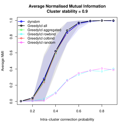
It appears that the greedy optimisation coupled with kmeans initialisations and dynsbm achieve the best results, whereas the greedy optimisation with random intialisations perform poorly. The average computing times are provided in Table 2.

Table 2: Simulation study. Average computing time required by each of the algorithms to be run on a generated dynamic network. Note that the variational expectation-maximisation of dynsbm and the greedy updates of our algorithm are both run exactly $4$ times for each dataset. The initialisation may be different, but we find that this does not impact the computing time by much.

Algorithm	Average computing time (seconds)
dynsbm	35.46
GreedyIcl all	4.58
GreedyIcl aggregated	1.18
GreedyIcl colbind	1.19
GreedyIcl rowbind	1.14
GreedyIcl random	1.07

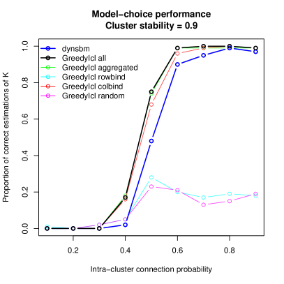
As concerns model selection, our methodology outperforms the existing algorithm of [13], as shown in Figure 3.

Figure 3: Simulation study. For each combination of $\pi$ and $\theta_{0}$, the proportion of networks where $K$ is properly estimated is shown, for all of the algorithms considered.

7 Enron dataset

The data.

The Enron Corporation filed for bankruptcy in late 2001, leading to an unprecedented scandal and to dire consequences for the US stock market. The data we use in this paper consists of all the emails exchanged from January 2000 to March 2002 between the Enron members. This data was originally made public, and posted to the web, by the Federal Energy Regulatory Commission during its investigation.

We construct a binary directed dynamic network of emails transforming the data into an adjacency cube $\mathcal{X}$, such that:

$$x_{ij}^{(t)}=\begin{cases}1,&\mbox{ at least an email is sent from member $i$ to member $j$ at time frame $t$;}\\ 0,&\mbox{ otherwise.}\\ \end{cases}$$ (21)

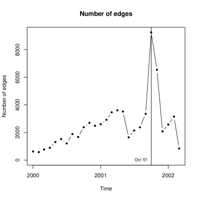
with each time frame $t$ corresponding to a one month period. The number of nodes is $N=148$ and the number of time frames is $T=27$. The number of edges observed at each time is shown in Figure 4.

Figure 4: Number of edges at each time frame for the Enron email dataset. The peak in October 2001 corresponds to the disclosure of bankruptcy.

Along with the email data, the status of each member within the company is known, and is one of the following: CEO, Director, Employee, In House Lawyer, Manager, Managing Director, N/A, President, Trader, Vice President. To simplify the exposition of the results, we gather every status other than Employee and N/A into a single class named Manager, so that only three status classes are considered.

We run our GreedyIcl all algorithm as in the simulation study, with each single run of the algorithm taking on average about $400$ seconds. The overall best solution has $17$ groups. An analysis of this clustering solution follows.

Activity levels and connectivity.

As shown in the left panel of Figure 5, the clustering solution has very high stability over time, in that nodes do not change allocations frequently.

Figure 5: Enron dataset. On the left panel, the estimated transition probabilities are shown. It appears that the network is very stable over time, and nodes tend not to change their allocations often. On the right panel, the estimated connection probabilities are shown. Most groups have high within cluster connectivity, although a number of off-diagonal entries are also relevant. The groups are ordered according to their aggregated size (i.e. the sum of their sizes over all times), in descending order. Some entries cannot be properly estimated due to a small cluster size, hence are left blank.

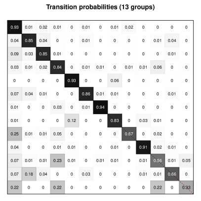
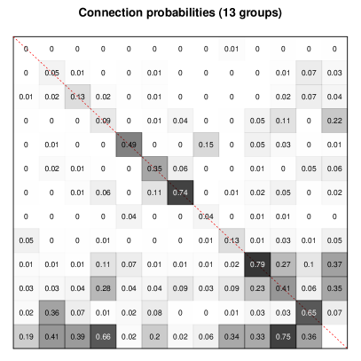
The connection probability matrix, shown on the right panel, exhibits instead a much more complex situation. Evidently, a strong community structure is present, since most of the diagonal elements of this matrix are fairly large.

We propose a brief characterisation of the role played by each group, using the information provided by this connection probability matrix, in conjunction with Tables 3, 4 and 5.

• Group 1: this group contains inactive nodes only. These members do not send emails, but they may receive a few newsletters.

• Groups 2 to 8: these contain a massive portion of the nodes, and hence describe the most common connectivity profiles that may arise. The nodes in these groups are not particularly active (the connection probabilities are typically not large) and tend to receive more emails than they send. The sizes of these groups swell increasingly by acquiring nodes from group 1 until the bankruptcy, signalling increased activity in the months before the default.

• Groups 9, 11, 12, 13: these groups are mainly composed of managers, and correspond to active nodes, who send more than they receive. These groups represent the different profiles of the executives of the company. Also note that these groups have a high within cluster connectivity, hence it is reasonable to find the corresponding conversations particularly meaningful in terms of intelligence and company directives.

• Groups 10, 14, 15: three groups of very active nodes, although these are mainly composed of employees. Note that groups 10 and 15 only become relevant during the year 2001.

• Group 16: this group actually only ever contains one person (with a non-specified role). This person apparently has some special position and hence may be considered as an outlier.

• Group 17: the smallest of groups, containing 4 unique members, each for $1$ time-frame only. Since this group has high connection probabilities towards many groups, it is reasonable to believe that nodes join this group whenever they send out newletters to all members.

Table 3: Rounded average degrees for the Enron dataset, for each of the $17$ clusters found.

	1	2	3	4	5	6	7	8	9	10	11	12	13	14	15	16	17
Avg. out-degree	0	3	3	1	3	4	3	5	5	3	7	10	13	12	11	11	57
Avg. in-degree	1	3	3	3	4	5	4	5	4	2	6	5	7	7	5	7	2

Table 4: Cluster counts separated by status for the Enron dataset. For this table, the same node at two different time frames is considered as two separate entities, hence the sum of all entries is $TN$.

	1	2	3	4	5	6	7	8	9	10	11	12	13	14	15	16	17
Employee	576	90	36	45	92	50	61	22	7	46	1	18	0	17	18	0	1
Manager	1027	231	191	102	34	83	53	16	89	40	87	45	41	6	5	0	2
N/A	475	57	27	50	59	40	12	84	2	9	4	5	2	16	5	16	1

Table 5: Group sizes at each time step for the Enron dataset.

Date	1	2	3	4	5	6	7	8	9	10	11	12	13	14	15	16	17
2000-01-01	115	8	3	2	1	2	5	4	2	0	2	0	1	2	0	1	0
2000-02-01	114	5	6	2	1	2	5	4	2	0	3	1	0	2	0	1	0
2000-03-01	112	5	7	3	2	2	4	4	2	0	3	1	0	2	0	1	0
2000-04-01	107	5	8	4	4	3	4	3	2	0	3	1	0	3	0	1	0
2000-05-01	103	7	6	6	5	3	4	2	2	0	3	2	1	3	0	1	0
2000-06-01	96	10	7	6	6	3	5	3	2	1	3	2	1	2	0	1	0
2000-07-01	93	10	6	5	5	4	5	3	3	1	5	3	1	2	1	1	0
2000-08-01	87	14	4	5	6	5	4	4	3	2	6	3	2	2	0	1	0
2000-09-01	86	13	5	6	7	4	4	5	2	2	5	3	2	2	1	1	0
2000-10-01	79	16	7	5	8	5	5	5	3	0	5	4	2	2	1	1	0
2000-11-01	71	15	7	5	8	5	5	5	6	6	4	4	2	2	2	1	0
2000-12-01	71	14	6	7	9	5	6	5	6	5	5	3	1	2	2	1	0
2001-01-01	72	14	8	7	9	4	7	5	3	4	3	4	2	2	3	1	0
2001-02-01	68	17	7	8	10	5	7	5	3	4	3	3	2	2	3	1	0
2001-03-01	69	15	7	9	11	5	5	6	3	4	3	3	3	1	3	1	0
2001-04-01	61	18	10	8	10	6	4	6	4	6	3	4	4	1	2	1	0
2001-05-01	52	21	15	8	11	7	4	7	3	6	3	4	4	0	2	0	1
2001-06-01	58	17	19	10	9	7	4	7	3	6	4	1	1	1	1	0	0
2001-07-01	67	13	13	9	6	8	4	5	5	7	4	3	2	1	1	0	0
2001-08-01	58	15	13	10	9	9	4	5	5	7	4	3	3	1	1	0	1
2001-09-01	50	19	16	10	10	11	5	5	5	7	4	4	1	0	1	0	0
2001-10-01	42	25	16	11	10	11	5	5	5	7	4	4	1	0	1	0	1
2001-11-01	41	26	17	11	10	11	5	5	6	6	3	4	1	1	1	0	0
2001-12-01	56	20	17	12	6	11	4	4	6	4	3	2	1	1	1	0	0
2002-01-01	64	20	14	10	3	11	3	5	5	5	2	1	3	1	1	0	0
2002-02-01	78	13	9	9	5	11	5	2	5	5	1	1	2	1	0	0	1
2002-03-01	108	3	1	9	4	13	4	3	2	0	1	0	0	0	0	0	0

Temporal dynamics.

Our model allows for groups to become inactive, whenever their sizes decrease to zero. This means that the connection profile associated to a particular group is not exhibited by any of the nodes in the time frame considered. Hence, the number of non-empty groups can be used as a measure of heterogeneity in the network, and the temporal dynamics of this quantity can be used to assess how heterogeneity evolves over time. In the left panel of Figure 6, the evolution of the number of non-empty groups is shown.

Figure 6: Enron dataset. On the left panel, the evolution of the number of non-empty groups is shown. This quantity appears to increase until the collapse, signalling an increase in heterogeneity in the network. On the right panel, the proportions of managers and employees allocated to the first group are shown. These proportions correspond to the nodes that are not particularly active.

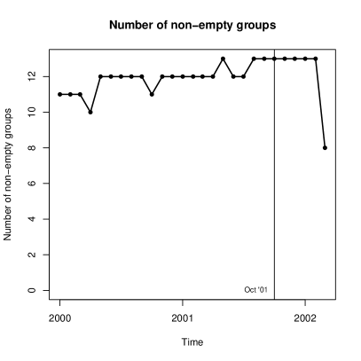
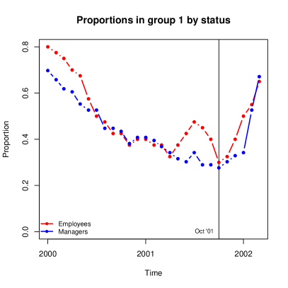
It appears that the network is particularly heterogeneous in the year before the collapse ($K^{(t)}=15$ or $16$), whereas it eventually becomes rather homogeneous ($K^{(t)}=10$) after the default. A similar message is conveyed by the plot on the right panel of Figure 6. Here the number of inactive nodes (i.e. nodes allocated to group 1) is shown to decrease convincingly for both employees and managers. Eventually, after the collapse, the first group is repopulated as members quit their jobs and activities.

8 London bike sharing

Data obtained from bike sharing systems is particularly suited to perform network analysis. Statistical analysis of the flows of bikes may provide important information regarding the management of the system and could help increase the efficiency of the service. Cycle hires data can be easily rearranged and visualised as a dynamic network structure, where edges correspond to hires and nodes to stations. Similar approaches have been recently proposed in a number of works, such as: [9], [18] and [14]. In a similar fashion, here we propose an application of our methodology to a dataset of cycle hires in London.

The data.

The cycle hire data for the London bike sharing system is publicly available from [21]. We use here the data from Wednesday, 5 June 2013 to Wednesday, 12 June 2013 (included). The discrete time frames correspond to blocks of three hours. For each time frame, we create a network adjacency matrix by transmuting bike trips into directed edges: an edge from station $i$ to station $j$ appears at time frame $t$ if at least one bike is hired at station $i$ during the corresponding three hours, and the same bike is then returned to station $j$. Bikes may be returned to the same station where they were hired: we consider this information not important for our analysis and hence discard all of the self-edges. The dynamic network so obtained is made of $N=566$ nodes and $T=64$ time frames. The data exhibits a very strong temporal heterogeneity, mainly due to the day-night cycle and the presence of the weekend days. In Figure 7 the observed number of edges is shown at every time frame.

Figure 7: The number of edges in each time frame for the London bikes dataset are shown on the left panel. The right panel shows instead the total number of edges in each day.

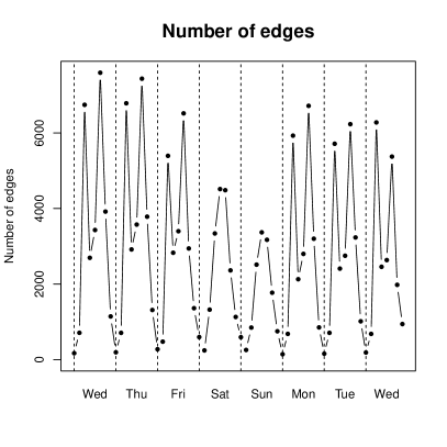
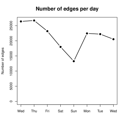
Weekdays typically exhibit two peaks in the activity level, corresponding to the start and the end of office hours. This suggests that commuters are the main users during working days. By contrast, low activity is observed throughout the weekend, with a single activity peak appearing in the late mornings.

Results.

We run our algorithm GreedyIcl once for each of the initialisation methods, with each run taking about six hours long. The optimal clustering found has a total of $K=43$ groups.

Heterogeneity.

The temporal dynamic of the activity level is also exhibited in Figure 8 by the number of active groups at each time frame: as in the Enron dataset, we use this as a measure for the level of heterogeneity in the network.

Figure 8: This plot shows the number of non-empty groups at each time frame for the London bikes dataset. The total number of unique groups found is $43$. The level of heterogeneity in the network has a noticeable temporal dynamic, which mimics the evolution of the number of links shown in Figure 7.

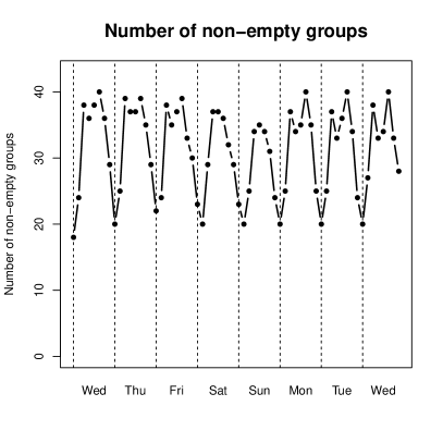
It appears that, as activity peaks in weekdays, the number of active groups doubles, signaling a heavy increase in heterogeneity within the network. Surprisingly, weekend days do not exhibit a markedly different heterogeneity level with respect to weekdays, even though the overall activity level is lower. This suggests that fewer nodes become active in the weekend, but their connection patterns are not particularly different than those seen in weekdays.

Characterisation of the groups.

The groups can be roughly divided in two categories: the first $20$ groups have a large aggregated size, mostly high stability, low connection probabilities and a good balance between expected out-degree and in-degree. The rest of the groups have smaller sizes, high instability, higher connection probabilities and in some cases very unbalanced out-degrees and in-degrees.

Figure 9 shows the temporal evolution of the size of a selection of groups.

Figure 9: London bikes data. Temporal dynamics for the sizes of some of the groups found. The three groups on the upper row belong to the first category (groups containing mostly inactive nodes): group 2 swells consistently every night; group 6 is stably present throughout; whereas group 12 is almost emptied in every weekday at the start of the office hours. The groups on the lower row contain instead very active stations: group 18 is emptied every night; group 21 is also emptied throughout the weekends; whereas group 33 activates every weekday at the start of office hours.

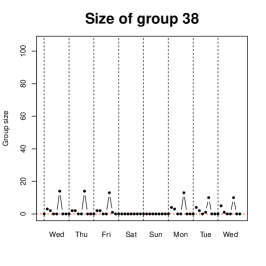
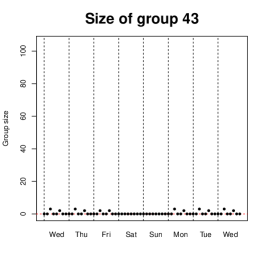
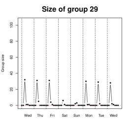
It appears that the trends in the activity level have a huge effect on the migrations of stations between groups. As nodes become more active, they leave the large groups (first category) and move to smaller groups, which are better suited to capture the details of their new connection profile in the network. During the high-activity regime these nodes may end up visiting several groups based on the evolution of their connectivity patterns. Nonetheless a good portion of nodes is not affected by the variation of activity level and simply remains stably in the larger and inactive groups.

These arguments are very well supported by the plots in Figure 10.

Figure 10: Stability level in the London bikes dataset. The left panel shows that although a good portion of nodes are very stable, there are some stations changing their allocations in more than 45 out of 64 time frames. The plot on the right hand side studies instead the stability of groups. It appears that larger groups are very stable, and viceversa smaller groups are not. The size of the circles is proportional to the size of the group aggregated over time.

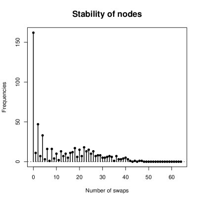
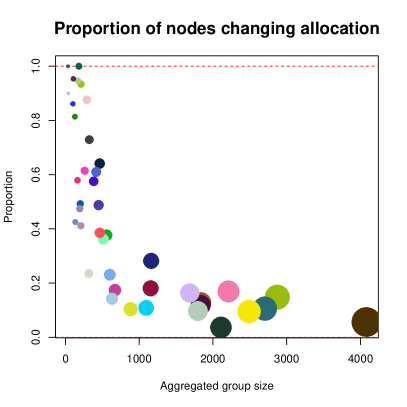
It appears that the stability of nodes is very heterogeneous in that there are many very stable nodes but also some very unstable ones (left panel). At the same time, the plot on the right hand side reinforces the idea that larger groups are also very stable whereas smaller groups exhibits high instability.

As shown in Figure 11 the stability does not seem to be particularly related to the geographical position of stations.

Figure 11: On the left panel, the spatial distribution of the stations not changing allocations is shown for the London bikes dataset. The colour of the circles correspond to the group they are allocated to at every time frame. On the right panel, instead, the stations performing more than 35 swaps are shown. In both plots the size corresponds to a combination of the out-degree and in-degree of the nodes.

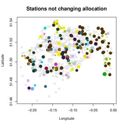
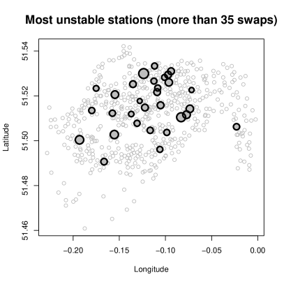
Furthermore, the number of groups containing stable stations (nodes that never change allocation) is relatively high.

One additional feature that distinguishes the two categories of groups found can be observed in Figure 12.

Figure 12: Expected out-degree versus expected in-degree for the groups found in the London bikes dataset. The size of circles is proportional to the size of groups aggregated over time. All of the large groups of inactive nodes have balanced degrees, in that they tend to send and receive the same number of edges. Smaller groups, instead, can exhibit very unbalanced degrees, either in favour of the out-degree or in-degree.

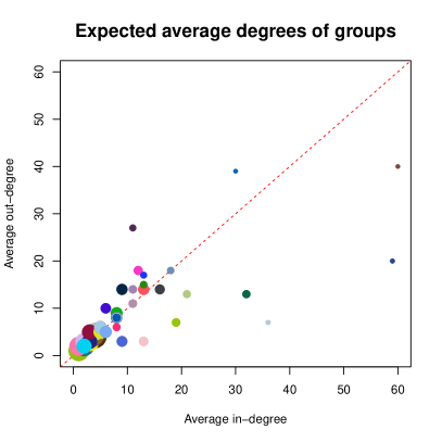
Here, for every group, the expected out-degrees versus the expected in-degrees are plotted. While stable groups (first category) tend to exhibit a good balance between the two degrees, smaller and unstable groups can also have very unbalanced degrees. This means, evidently, that whenever a node joins one of this unbalanced groups, it may send many more edges than what it receives (or viceversa). In this bike sharing context, the corresponding stations may require special attention due to temporary excess of hiring demands (or excess of arrivals).

9 Conclusions

The statistical analysis of dynamic networks is particularly challenging, both from a modelling point of view (due to the temporal dynamics) and from an estimation point of view, due to the inherent computational difficulties. In this paper we have focused on an extension of the stochastic block model to dynamic networks, where the temporal evolution of the nodal information is captured by a Markovian process. Our formulation allows one to integrate out all of the model parameters from both the likelihood and the prior, thereby obtaining an analytical formula for the marginal posterior of the allocation variables. In a model-based clustering context, such a marginal posterior is equivalent to the exact integrated completed likelihood, which is widely used as an optimality criterion for partitions.

Taking advantage of these results, we have proposed a greedy algorithm to estimate the optimal clustering of the nodes. Our algorithm resembles other tools proposed in the recent literature, and scales particularly well with the size of the data. However, only convergence to a local optimum is guaranteed, hence several restarts and a careful initialisation are particularly useful in order to find the global optimum.

One appealing feature of our approach is that model-choice is carried out automatically, since the number of groups can be deduced at each time frame from the optimal clustering solution.

Through a simulation study, we have validated both our optimality criterion and the greedy algorithm used to estimate the optimal partition. Also, we have compared our method to one based on a variational Expectation-Maximisation algorithm, showing that with careful initialisation our approach achieves better results when the underlying number of groups is unknown.

We have applied our methodology to the Enron email dataset, and found $17$ underlying groups. Each of the groups found appears to have a specific role within the network and the original status of the members seem to be particularly related with the nodes’ allocations. Also, we have analysed some relevant summaries from our optimal clustering underlining the dynamic evolution of the heterogeneity within the network and of the overall activity level.

We have also applied our methodology to a London Bikes dataset, to study the flows and connections between bike stations. Our method has returned an optimal clustering made of $43$ groups. The analysis of such a complex structure has been particularly challenging but we have managed to extract some interesting information regarding the dynamics captured by the model.

We note that, while the practice of integrating out the likelihood parameters has been exploited in a number of recent papers, the collapsing of the transition probabilities in the Markov process is a rather new original technique. Not only this creates an ideal setup for our method, but it may also be generalised and exploited in arbitrary discrete hidden Markov models and their extensions.

Additionally, our work may be extended in a number of ways. We have used our algorithm only on binary networks, but this approach generalises to networks with other edge types. Incomplete weighted graphs can be easily handled using a Bernoulli presence-absence indicator, and hence using the same framework based on the collapsing of the parameters.

The initialisation plays an important role in our method, yet finding a good starting partition is a great challenge. In fact, there is a lack of scalable methods that can handle complex dynamic objects such as networks. Furthermore, clustering cannot be attempted for each time frame independently since this result in label-switching problems. Here, we have proposed two new intialisation methods which may in some cases improve the results.

Extensions to the supervised classification case are also straightforward: if some of the allocations are known, these need not be updated during the greedy optimisation. From a Bayesian perspective, the optimal clustering solution obtained will then maximise the posterior predictive distribution, rather than the posterior. This strategy would be useful when dealing with nodes that join or leave the study dynamically, since, as suggested by [13], a fixed group of inactive nodes may be created.

More generally, the optimisation of the exact Integrated Completed Likelihood is a particularly challenging task, due to the discrete search space and the pronounced multimodality of such objective function. The GreedyIcl algorithm introduced in this paper was shown to perform well, although future extensions may improve upon our work in terms of efficiency using alternative optimisation routines.

References

- [1] E. M. Airoldi, D. M. Blei, S. E. Fienberg and E. P. Xing “Mixed membership stochastic blockmodels” In Journal of Machine Learning Research 9, 2008, pp. 1981–2014
- [2] M. Bertoletti, N. Friel and R. Rastelli “Choosing the number of clusters in a finite mixture model using an exact integrated completed likelihood criterion” In Metron 73.2 Springer, 2015, pp. 177–199
- [3] J. Besag “On the statistical analysis of dirty pictures” In Journal of the Royal Statistical Society. Series B (Methodological) 48.3 JSTOR, 1986, pp. 259–302
- [4] C. Biernacki, G. Celeux and G. Govaert “Assessing a mixture model for clustering with the integrated completed likelihood” In Pattern Analysis and Machine Intelligence, IEEE Transactions on 22.7 IEEE, 2000, pp. 719–725
- [5] E. Côme and P. Latouche “Model selection and clustering in stochastic block models based on the exact integrated complete data likelihood” In Statistical Modelling SAGE Publications, 2015, pp. 1471082X15577017
- [6] M. Corneli, P. Latouche and F. Rossi “Exact ICL maximization in a non-stationary temporal extension of the stochastic block model for dynamic networks” In Neurocomputing 192 Elsevier, 2016, pp. 81–91
- [7] J. J. Daudin, F. Picard and S. Robin “A mixture model for random graphs” In Statistics and Computing 18.2 Springer, 2008, pp. 173–183
- [8] N. Friel, R. Rastelli, J. Wyse and A. E. Raftery “Interlocking directorates in Irish companies using a latent space model for bipartite networks” In Proceedings of the National Academy of Sciences 113.24, 2016, pp. 6629–6634
- [9] R. Guigourès, M. Boullé and F. Rossi “Discovering patterns in time-varying graphs: a triclustering approach” In Advances in Data Analysis and Classification Springer, 2015, pp. 1–28
- [10] Q. Ho, L. Song and E. P. Xing “Evolving cluster mixed-membership blockmodel for time-evolving networks” In International Conference on Artificial Intelligence and Statistics, 2011, pp. 342–350
- [11] P. D. Hoff, A. E. Raftery and M. S. Handcock “Latent space approaches to social network analysis” In Journal of the American Statistical Association 97.460 Taylor & Francis, 2002, pp. 1090–1098
- [12] M. Kim and J. Leskovec “Nonparametric multi-group membership model for dynamic networks” In Advances in Neural Information Processing Systems (25), 2013, pp. 1385–1393
- [13] C. Matias and V. Miele “Statistical clustering of temporal networks through a dynamic stochastic block model” In Journal of the Royal Statistical Society: Series B (Statistical Methodology), 2016, pp. n/a–n/a DOI: 10.1111/rssb.12200
- [14] C. Matias, T. Rebafka and F. Villers “A semiparametric extension of the stochastic block model for longitudinal networks” In HAL-preprint, 2016
- [15] A. F. McDaid, T. B. Murphy, N. Friel and N. J. Hurley “Improved Bayesian inference for the stochastic block model with application to large networks” In Computational Statistics & Data Analysis 60 Elsevier, 2013, pp. 12–31
- [16] M. E. J. Newman “Fast algorithm for detecting community structure in networks” In Physical review E 69.6 APS, 2004, pp. 066133
- [17] K. Nowicki and T. A. B. Snijders “Estimation and prediction for stochastic blockstructures” In Journal of the American Statistical Association 96.455 Taylor & Francis, 2001, pp. 1077–1087
- [18] A. N. Randriamanamihaga, E. Côme, L. Oukhellou and G. Govaert “Clustering the Velib dynamic Origin/Destination flows using a family of Poisson mixture models” In Neurocomputing 141 Elsevier, 2014, pp. 124–138
- [19] P. Sarkar and A. W. Moore “Dynamic social network analysis using latent space models” In SIGKDD Explorations: Special Edition on Link Mining 7, 2005, pp. 31–40
- [20] A. Strehl and J. Ghosh “Cluster ensembles – a knowledge reuse framework for combining multiple partitions” In The Journal of Machine Learning Research 3 JMLR. org, 2003, pp. 583–617
- [21] “Transport for London” http://cycling.data.tfl.gov.uk/., 2016
- [22] Y. J. Wang and G. Y. Wong “Stochastic blockmodels for directed graphs” In Journal of the American Statistical Association 82, 1987, pp. 8–19
- [23] J. Wyse, N. Friel and P. Latouche “Inferring structure in bipartite networks using the latent block model and exact ICL” In Network Science (to appear), 2017
- [24] Eric P. Xing, Wenjie Fu and Le Song “A state-space mixed membership blockmodel for dynamic network tomography” In Ann. Appl. Stat. 4.2 The Institute of Mathematical Statistics, 2010, pp. 535–566 DOI: 10.1214/09-AOAS311
- [25] K. S. Xu and A. O. Hero “Dynamic stochastic blockmodels for time-evolving social networks” In Selected Topics in Signal Processing, IEEE Journal of 8.4 IEEE, 2014, pp. 552–562
- [26] T. Yang, Y. Chi, S. Zhu, Y. Gong and R. Jin “Detecting communities and their evolutions in dynamic social networks – a Bayesian approach” In Machine learning 82.2 Springer, 2011, pp. 157–189