Sparse Representation of Gravitational Sound

Abstract

Gravitational Sound clips produced by the Laser Interferometer Gravitational-Wave Observatory (LIGO) and the Massachusetts Institute of Technology (MIT) are considered within the particular context of data reduction. We advance a detailed procedure to this effect and show that these types of signals can be approximated with high quality using significantly fewer elementary components than those required within the standard orthogonal basis framework. Furthermore, a measure a local sparsity is shown to render meaningful information about the variation of a signal along time, by generating a set of local sparsity values which is much smaller than the dimension of the signal. This point is further illustrated by recourse to a more complex signal, generated by Milde Science Communication to divulge Gravitational Sound in the form a ring tone.

1 Introduction

In 1905 Henri Poincaré first suggested that accelerated masses in a relativistic field should produce gravitational waves [1]. The idea was magisterially pursued by Einstein via his celebrated theory of general relativity. In 1918 he published his famous quadrupole formula resulting from the calculation of the effect of gravitational waves [2]. A century later, the LIGO Scientific Collaboration and Virgo Collaboration published a paper about the gravitational radiation they had detected on September 2015 [3]. Ever since scientists believe to have entered in a new era of astronomy, whereby the universe will be studied by ‘its sound’ [4, 5, 6, 7, 8]. Gravitational Sound (GS) signals will then be here scrutinized with advanced techniques.

In the signal processing field, the problem of finding a sparse approximation for a signal consists in expressing the signal as a superposition of as few elementary components as possible, without significantly affecting the quality of the reconstruction. In signal processing applications the approximation is carried out on a signal partition, i.e., by dividing the signal into small pieces and constructing the approximation for each of those pieces of data. Traditional techniques would carry out the task using an orthogonal basis. However, enormous improvements in sparsity can be achieved using an adequate over-complete ‘dictionary’ and an appropriate mathematics method. For the most part, these methods are based on minimization of the $l_{1}$-norm [9] or are greedy pursuit strategies [10, 11, 12, 13, 14, 15, 16, 17], the latter being much more effective in practice.

Sparse signal representation of sound signals is a valuable tool for a number of auditory tasks [18, 19]. Moreover, the emerging theory of compressive sensing [20, 21, 22] has enhanced the concept of sparsity by asserting that the number of measurements needed for accurate representation of a signal informational content decreases if the sparsity of the representation improves. Hence, when some GS tones made with the observed Gravitation Wave (GW) were released, we felt motivated to produce a sparse approximation of those clips.

We simply analyze the GS tones from a processing viewpoint, regardless on how and why they have been generated. We consider a) a short tone made with the chirp gw151226 that has been detected, b) the theoretical simulated theoretical GS, iota_20_10000_4_4_90_h, and c) the Black_Hole_Billiards ring tone, which is a more complex signal produced by superposition with an ad hoc independent percussive sound. The ensuing results are certainly interesting. If, in the future, GS signals are to be generated at large scale (as astronomical images have been produced [24, 23]), it is important to have tools for all kinds of processing of those signals.

The central goal of this Communication is to present evidences of the significant gain in sparsity achieved if a GS signal is approximated with high quality outside the orthogonal basis framework. For demonstration purposes we have made available the MATLAB routines for implementation of the method.

2 Some Preliminary Considerations

The traditional frequency decomposition of a signal given by $N$ sample points, $f(i),\,i=1,\ldots,N$, involves the Fourier expansion $f(i)=\frac{1}{\sqrt{N}}\sum_{n=1}^{M}c(n)e^{\imath\frac{2\pi(i-1)(n-1)}{M}},\quad i=1,\ldots,N.$ The values $|c(n)|,\,n=1,\ldots,M=N$ are called the discrete Fourier spectrum of the signal, and can be evaluated in a very effective manner via the Fast Fourier Transform (FFT). For $M>N$ even if the coefficients in the above expansion can still be calculated via FFT, by zero padding, these are not longer unique. Finding a sparse solution is the goal of sparse approximation techniques.

The problem of the sparse approximation of a signal, outside the orthogonal basis setting, consists in using elements of a redundant set, called a dictionary, for constructing an approximation involving a number of elementary components which is significantly smaller than the signal dimension. For signals whose structure varies with time, sparsity performs better when the approximation is carried out on a signal partition. In order to give precise definitions we introduce at this point the notational usual conventions: $\mathbb{R}$ and $\mathbb{C}$ represent the sets of real and complex and numbers, respectively. Boldface fonts are used to indicate Euclidean vectors and standard mathematical fonts to indicate components, e.g., $\mathbf{d}\in\mathbb{C}^{N}$ is a vector of $N$-components $d(i)\in\mathbb{C}^{N}\,,i=1,\ldots,N$. The operation $\langle\cdot,\cdot\rangle$ indicates the Euclidean inner product and $\|\cdot\|$ the induced norm, i.e. $\|\mathbf{d}\|^{2}=\langle\mathbf{d},\mathbf{d}\rangle$, with the usual inner product definition: For $\mathbf{d}\in\mathbb{C}^{N}$ and $\mathbf{f}\in\mathbb{C}^{N}$ $\langle\mathbf{f},\mathbf{d}\rangle=\sum_{i=1}^{N}f(i)d^{\ast}\!(i),$ where $d^{\ast}\!(i)$ stands for the complex conjugate of $d(i)$.

A partition of a signal $\mathbf{f}\in\mathbb{R}^{N}$ is represented as a set of disjoint pieces, $\mathbf{f}_{q}\in\mathbb{R}^{N_{b}},\,q=1,\ldots,Q$, henceforth to be called ‘blocks’, which, without loss of generality, are assumed to be all of the same size and such that $QN_{b}=N$. Denoting by $\hat{\operatorname{J}}$ the concatenation operator, the signal $\mathbf{f}\in\mathbb{R}^{N}$ is ‘assembled’ from the blocks as $\mathbf{f}=\hat{\operatorname{J}}_{q=1}^{Q}\mathbf{f}_{q}$. This operation implies that the first $N_{1}$ components of the vector $\mathbf{f}$ are given by the vector $\mathbf{f}_{1}$, the next $N_{2}$ components by the vector $\mathbf{f}_{2}$, and so on.

A dictionary for $\mathbb{R}^{N_{b}}$ is an over-complete set of (normalized to unity) elements $\mathcal{D}=\{\mathbf{d}_{n}\in\mathbb{R}^{N_{b}}\,;\|\mathbf{d}_{n}\|=1\}_{n=1}^{M},$ which are called atoms.

3 Sparse Signal Approximation

Given a signal partition $\mathbf{f}_{q}\in\mathbb{R}^{N_{b}},\,q=1,\ldots,Q$ and a dictionary $\mathcal{D}$, the $k_{q}$-term approximation for each block is given by an atomic decomposition of the form

$$\mathbf{f}^{k_{q}}_{q}=\sum_{n=1}^{k_{q}}c^{k_{q}}(n)\mathbf{d}_{\ell^{q}_{n}},\quad q=1,\ldots,Q.$$ (1)

The approximation to the whole signal is then obtained simply by joining the approximation for the blocks as $\mathbf{f}^{K}=\hat{\operatorname{J}}_{q=1}^{Q}\mathbf{f}^{k_{q}}_{q},$ where $K=\sum_{q=1}^{Q}k_{q}$.

3.1 The Method

The problem of finding the minimum number of $K$ terms such that $\|\mathbf{f}-\mathbf{f}^{K}\|<\rho$, for a given tolerance parameter $\rho$, is an NP-hard problem [12]. In practical applications, one looks for tractable sparse solutions. For this purpose we consider the Optimized Hierarchical Block Wise (HBW) version [25] of the Optimized Orthogonal Matching Pursuit (OOMP) [13] approach. This entails that, in addition to selecting the dictionary atoms for the approximation of each block, the blocks are ranked for their sequential stepwise approximation. As a consequence, the approach is optimized in the sense of minimizing, at each iteration step, the norm of the total residual error $\|\mathbf{f}-\mathbf{f}^{K}\|$ [25]. As will be illustrated in Sec. 3.3, when approximating a signal with pronounced amplitude variations the sparsity result achieved by this strategy is remarkable superior to that arising when the approximation of each block is completed at once, i.e., when the ranking of blocks is omitted. The OHBW-OOMP method is implemented using the steps indicated below.

OHBW-OOMP Algorithm

• For $q=1,\ldots,Q$ initialize the algorithm by setting: $\mathbf{r}_{q}^{0}=\mathbf{f}_{q}$, $\mathbf{f}_{q}^{0}=0$, $\Gamma_{q}=\emptyset$ $k_{q}=0$, and selecting the ‘potential’ first atom for the atomic decomposition of every block $q$ as the one corresponding to the indexes $\ell_{1}^{q}$ such that

  $$\ell_{1}^{q}=\operatorname*{arg\,max}_{n=1,\ldots,M}\left|\langle\mathbf{d}_{n},\mathbf{r}_{q}^{k_{q}}\rangle\right|^{2},\quad q=1,\ldots,Q.$$ (2)

  Assign $\mathbf{w}_{1}^{q}=\mathbf{b}_{1}^{q}=\mathbf{d}_{\ell_{1}^{q}}$.

• Use the OHBW criterion for selecting the block to upgrade the atomic decomposition by adding one atom

  $$q^{\star}=\operatorname*{arg\,max}_{q=1,\ldots,q}\frac{|\langle\mathbf{w}_{k_{q}+1}^{q},\mathbf{f}_{q}\rangle|^{2}}{\|\mathbf{w}_{k_{q}+1}^{q}\|^{2}}.$$ (3)

  If $k_{{q^{\star}}}>0$ upgrade vectors $\{\mathbf{b}_{n}^{k_{q^{\star}},{q^{\star}}}\}_{n=1}^{k_{q^{\star}}}$ for block ${q^{\star}}$ as

  $$\begin{split}\mathbf{b}_{n}^{{k_{q^{\star}}}+1,{q^{\star}}}&=\mathbf{b}_{n}^{{k_{q^{\star}}},{q^{\star}}}-\mathbf{b}_{k_{q^{\star}}+1}^{{k_{q^{\star}}}+1,{q^{\star}}}\langle\mathbf{d}_{\ell_{{k_{q^{\star}}}+1}}^{{q^{\star}}},\mathbf{b}_{n}^{k_{q^{\star}}+1,{q^{\star}}}\rangle,\quad n=1,\ldots,k_{q},\\ \mathbf{b}_{k_{q^{\star}}+1}^{k_{q^{\star}}+1,{q^{\star}}}&=\frac{\mathbf{w}_{k_{q^{\star}}+1}^{q^{\star}}}{\|\mathbf{w}_{k_{q^{\star}}+1}^{q^{\star}}\|^{2}}.\end{split}$$ (4)

• Calculate

  $$\mathbf{r}_{{q^{\star}}}^{k_{q^{\star}}+1} = \mathbf{r}_{q}^{k_{q^{\star}}}-\langle\mathbf{w}_{k_{q^{\star}}+1}^{{q^{\star}}},\mathbf{f}_{{q^{\star}}}\rangle\frac{\mathbf{w}_{k_{q^{\star}}+1}^{{q^{\star}}}}{\|\mathbf{w}_{k_{q^{\star}}+1}^{{q^{\star}}}\|^{2}},$$

  $$\mathbf{f}_{{q^{\star}}}^{k_{q^{\star}}+1} = \mathbf{f}_{{q^{\star}}}^{k_{q^{\star}}+1}+\langle\mathbf{w}_{k_{q^{\star}}+1}^{{q^{\star}}},\mathbf{f}_{{q^{\star}}}\rangle\frac{\mathbf{w}_{k_{q^{\star}}+1}^{{q^{\star}}}}{\|\mathbf{w}_{k_{q^{\star}}+1}^{{q^{\star}}}\|^{2}}.$$ (5)

  Upgrade the set $\Gamma_{{q^{\star}}}\leftarrow\Gamma_{{q^{\star}}}\cup\ell_{k_{q^{\star}}+1}$ and increase $k_{q^{\star}}\leftarrow k_{q^{\star}}+1$.

• Select a new potential atom for the atomic decomposition of block ${q^{\star}}$, using the OOMP criterion, i.e., choose $\ell_{k_{q^{\star}}+1}^{q}$ such that

  $$\ell_{k_{q^{\star}}+1}^{q}=\operatorname*{arg\,max}_{\begin{subarray}{c}n=1,\ldots,M\\ n\notin\Gamma_{q}\end{subarray}}\frac{|\langle\mathbf{d}_{n},\mathbf{r}_{{q^{\star}}}^{k_{q}}\rangle|^{2}}{1-\sum_{i=1}^{k_{q}}|\langle\mathbf{d}_{n},\tilde{\mathbf{w}}_{i}^{q}\rangle|^{2}},,\quad\text{with}\quad\tilde{\mathbf{w}}_{i}^{{q^{\star}}}=\frac{\tilde{\mathbf{w}}_{i}^{{q^{\star}}}}{\|\tilde{\mathbf{w}}_{i}^{{q^{\star}}}\|},$$ (6)

• Compute the corresponding new vector $\mathbf{w}_{k_{q^{\star}}+1}^{{q^{\star}}}$ as

  $$\begin{split}\mathbf{w}_{k_{q^{\star}}+1}^{q}=\mathbf{d}_{\ell_{k_{q^{\star}}+1}}^{q}-\sum_{n=1}^{k_{q^{\star}}}\frac{\mathbf{w}_{n}^{q^{\star}}}{\|\mathbf{w}_{n}^{q^{\star}}\|^{2}}\langle\mathbf{w}_{n}^{q^{\star}},\mathbf{d}_{\ell_{k_{q^{\star}}}}^{q}\rangle.\end{split}$$ (7)

  including, for numerical accuracy, the re-orthogonalizing step:

  $$\mathbf{w}_{k_{q^{\star}}+1}^{q}\leftarrow\mathbf{w}_{k_{q^{\star}}+1}^{q}-\sum_{n=1}^{k_{q^{\star}}}\frac{\mathbf{w}_{n}^{q^{\star}}}{\|\mathbf{w}_{n}^{q^{\star}}\|^{2}}\langle\mathbf{w}_{n}^{q^{\star}},\mathbf{w}_{k_{q^{\star}}+1}^{q}\rangle.$$ (8)

• Check if, for a given $K$ and $\rho$ either the condition $\sum_{q=1}^{Q}k_{q}=K+1$ or $\|\mathbf{f}-\mathbf{f}^{K}\|<\rho$ has been met. If that is the case, for $q=1,\ldots,Q$ compute the coefficients $c^{k_{q}}(n)=\langle\mathbf{b}_{n}^{k_{q}},\mathbf{f}_{q}\rangle,\,n=1,\ldots,k_{q}$. Otherwise repeat steps 2) - 5).

Remark 1: For all the values of $q$, the OOMP criterion (6) in the algorithm above ensures that, fixing the set of previously selected atoms, the atom corresponding to the indexes given by (6) minimizes the local residual norm $\|\mathbf{f}_{q}-\mathbf{f}_{q}^{k_{q}}\|$ [13]. Moreover, the OHBW-OOMP criterion (3), for choosing the block to upgrade the approximation, ensures the minimization of the total residual norm [25]. Let us recall that the OOMP approach optimizes the Orthogonal Matching Pursuit (OMP) one [11]. The latter is also an optimization of the plain Matching Pursuit (MP) method [10](see the discussion in [13]).

3.2 The Dictionary

The degree of success in achieving high sparsity using a dictionary approach depends on both, the suitability of the mathematical method for finding a tractable sparse solution and the dictionary itself. As in the case of melodic music [25, 26], we found the trigonometric dictionary $\mathcal{D}_{T}$, which is the union of the dictionaries $\mathcal{D}_{C}$ and $\mathcal{D}_{S}$ given below, to be an appropriate dictionary for approximating these GS signals.

$$\mathcal{D}_{C}^{x} = \{w_{c}(n)\cos{\frac{{\pi(2i-1)(n-1)}}{2M}},i=1,\ldots,N_{b}\}_{n=1}^{M}$$

$$\mathcal{D}_{S}^{x} = \{w_{s}(n)\sin{\frac{{\pi(2i-1)(n)}}{2M}},i=1,\ldots,N_{b}\}_{n=1}^{M}.$$

In the above sets $w_{c}(n)$ and $w_{s}(n),\,n=1,\ldots,M$ are normalization factors.

Figure 1: Prototype atoms $\mathbf{p}_{1},\mathbf{p}_{2}$ and $\mathbf{p}_{3}$, which generate the dictionaries $\mathcal{D}_{P1}$, $\mathcal{D}_{P1}$ and $\mathcal{D}_{P3}$ by sequential translations of one point. Each prototype is shown in a different color.

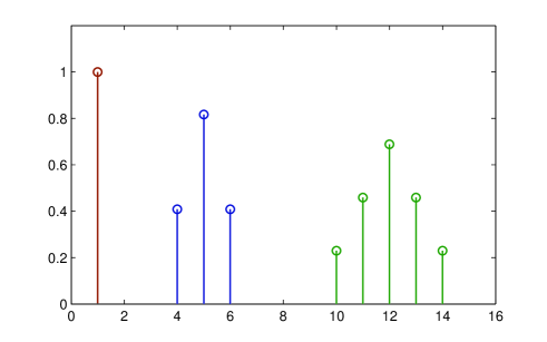
We also found that sparsity may benefit by the inclusion of a dictionary which is constructed by translation of the prototype atoms, $\mathbf{p}_{1},\mathbf{p}_{2}$ and $\mathbf{p}_{3}$ in Fig. 1. Denoting by $\mathcal{D}_{P_{1}}$, $\mathcal{D}_{P_{2}}$ and $\mathcal{D}_{P_{3}}$ the dictionaries arising by translations of the atoms $\mathbf{p}_{1}$, $\mathbf{p}_{2}$, and $\mathbf{p}_{3}$, respectively, the dictionary $\mathcal{D}_{P}$ is built as $\mathcal{D}_{P}=\mathcal{D}_{P_{1}}\cup\mathcal{D}_{P_{2}}\cup\mathcal{D}_{P_{3}}$. The whole mixed dictionary is then $\mathcal{D}_{M}=\mathcal{D}_{T}\cup\mathcal{D}_{P}$, with $\mathcal{D}_{T}=\mathcal{D}_{C}\cup\mathcal{D}_{S}$. Interestingly enough, the dictionary $\mathcal{D}_{M}$ happens to be a sub-dictionary of a larger dictionary proposed in [27] for producing sparse representations of astronomical images, the difference being that, in this case, sparsity does not improve in a significant way by further enlarging the dictionary.

From a computational viewpoint the particularity of the sub-dictionaries $\mathcal{D}_{C}$ and $\mathcal{D}_{S}$ is that the inner product with all its elements can be evaluated via FFT. This possibility reduces the complexity of the numerical calculations when the partition unit $N_{b}$ is large [25, 26]. Also, the inner products with the atoms of the dictionaries $\mathcal{D}_{P_{2}}$ and $\mathcal{D}_{P3}$ can be effectively implemented, all at once, via a convolution operation.
Note: The MATLAB routine implementing the OHBW-OOMP approach, dedicated to the dictionary introduced in this section, has been made available on [28].

3.3 The Processing

We process now the three signals we are considering here:

• The audio representation of the detected gw151226 chirp [29].

• The tone of the theoretical gravitational wave iota_20_10000_4_4_90_h [30].

• The Black_Hole_Billiards ring tone [29].

The quality of an approximation is measured by the Signal to Noise Ratio (SNR) which is defined as

$$\text{SNR}=10\log_{10}\frac{\|\mathbf{f}\|^{2}}{\|\mathbf{f}-\mathbf{f}^{K}\|^{2}}=10\log_{10}\frac{\sum_{\begin{subarray}{c}i=1\\ q=1\end{subarray}}^{N_{b},Q}|f_{q}(i)|^{2}}{\sum_{\begin{subarray}{c}i=1\\ q=1\end{subarray}}^{N_{b},Q}|f_{q}(i)-f^{k_{q}}_{q}(i)|^{2}}.$$ (9)

The sparsity of the whole representation is measured by the Sparsity Ratio (SR) defined as $\displaystyle{\text{SR}=\frac{N}{K}}$, where $K$ is the total number of coefficients in the signal representation as defined above.

Audio representation of the chirp gw151226

This clip, made with the detected short chirp gw151226, is plotted in the left graph of Fig.2. The graph on the right is its classic spectrogram.

Figure 2: The graph on the left represents the clip gw151226. The central line is the difference between the approximation, up to SNR=50dB, and the signal. The right graph is the classic spectrogram of the clip on the left.

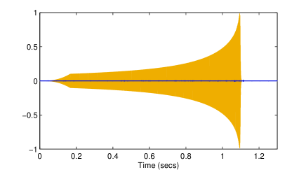
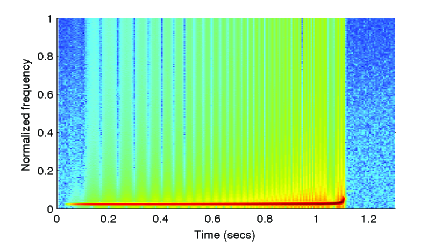
When an orthogonal basis for approximating these signals is used, the best sparsity result is achieved with the Discrete Cosine Transform (DCT). Hence, we first approximate this clip, up to SNR=50dB, by nonlinear thresholding of the DCT coefficients. The best SR (SR= 28.7) is obtained for $N_{b}=N=65536$, i.e., by processing the signal as a single block. Contrarily, when approximating the clip using the trigonometric dictionary $\mathcal{D}_{T}$, the best result is obtained for $N_{b}=2048$, achieving a much higher SR. Approximating each block at once, with the OOMP approach, SR=209.4, and raking the blocks with the OHBW-OOMP approach SR= 263.2. Let us stress that this implies a gain in sparsity result of $817\%$ with respect to the DCT approach for the same value of SNR. The central dark line in the left graph of Fig. 2 represents the difference between the signal and its approximation, up to SNR=50dB. For this chirp the inclusion of the dictionary $\mathcal{D}_{P}$ would not improve sparsity.

Theoretical Gravitational Wave Sound

This is the iota_20_10000_4_4_90_h gravitational wave, which belongs to the family of Extreme Mass Ratio Inspirals [31, 32, 33, 34, 35] available on [30].

Figure 3: The graph on the left represents the iota_20_10000_4_4_90_h tone. The central line is the difference between the approximation, up to SNR=50dB, and the signal. The right graph is the spectrogram of the clip on the left.

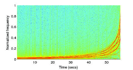
It consists of $N=458752$ data points plotted in the left graph of Fig. 3. The graph on the right is its classic spectrogram. In this case the best SR result (SR=5.1), produced by nonlinear thresholding of the DCT coefficients for approximating the signal up to SNR=50dB, is obtained with $N_{b}=16384$. A much smaller value of $N_{b}$ ($N_{b}=2048$) is required to achieve the best SR result (SR=10.8) with the OHBW-OOMP method and the trigonometric dictionary. With the mixed dictionary $\mathcal{D}_{M}$ there is a further improvement: SR=11.9. The central dark line in the left graph of Fig. 3 represents the difference between the signal and its approximation, up to SNR=50dB. For this signal the gain in SR with respect to the DCT approximation is $136\%$. Since the amplitude of the signal does not vary much along time, the SR obtained by approximating each block at once, with OOMP, does not significantly differ from the values obtained applying the OHBW-OOMP strategy.

The Black_Hole_Billiards ring tone

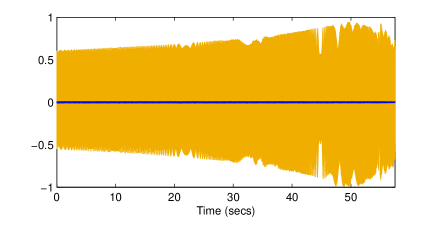
In order to stress the relevance of the technique for representing features of more complex signals using a very reduced set of points, we consider here Black_Hole_Billiards ring tone available on [29]. This clip was created by Milde Science Communication by superimposing a sound of percussive nature (the billiards sound) to a GW chirp. It consisting of $N=262144$ samples plotted in the left graph of Fig. 4.

Figure 4: The graph on the left represents the Black_Hole_Billiards clip. Credit: Milde Science Communication. The central dark line is the difference between the approximation, up to SNR=40dB, and the signal. The right graph is the spectrogram of the clip on the left.

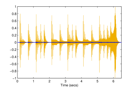
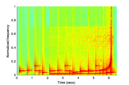
The graph on the right is its classic spectrogram. When processing the signal with DCT the best sparsity result when the approximation is carried out block by block up to the same error is SR=4.2, for SNR=40dB, and corresponds to $N_{b}=16384$. However, with $N_{b}=2048$ the OHBW version for selecting DCT coefficients improves in this case the standard DCT result, attaining SR=6.2. For an approximation of the same quality (SNR=40 dB) the SR rendered by the OHBW-OOMP method with $N_{b}=512$ and the trigonometric dictionary $\mathcal{D}_{T}$ is SR= 12.1. With the mixed dictionary $\mathcal{D}_{M}$ this value increases to SR=13.7. The central dark line in the left graph of Fig. 4 represents the difference between the signal and its approximation, up to SNR=40dB. It is worth commenting that, if with the same dictionary, the approximation were carried out without ranking the blocks, i.e., approximating each block at once up to the same SNR, the value of SR would be only 6.7. This example highlights the importance of adopting the OHBW strategy for constructing the signal approximation, when the signal amplitude varies significantly along the domain of definition.

3.4 The Role of Local Sparsity

The SR is a global measure of sparsity indicating the number of elementary components contained in the whole signal. An interesting description of a the signal variation is rendered by a local measure of sparsity. For this we consider the local sparsity ratio $sr(q)=\frac{N_{b}}{k_{q}},\,q=1,\ldots,Q$ where, as defined above, $k_{q}$ is the number of coefficients in the decomposition of the $q$-block and $N_{b}$ the size of the block.

Figure 5: The dark line in the left graph joins the inverse local sparsity values for the clip gw151226. The right graph has the same description but for the iota_20_10000_4_4_90_h clip. tone.

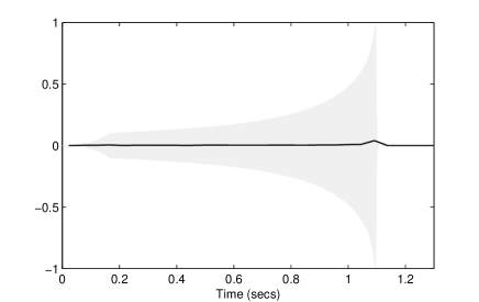
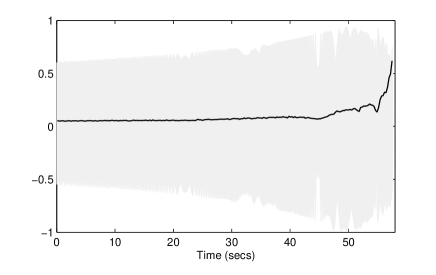
For illustration’s convenience the dark line in both graphs of Fig. 5 depicts the inverse of this local measure. This line joins the values $1/sr(q),\,q=1,\ldots,Q$. Each of these values is located in the horizontal axis at the center of the corresponding block and provides much information about the signal. Certainly, simply from the observation of the the dark line in the left graph of Fig. 5 (joining 32 points of inverse local sparsity ratio) one can realize that the number of internal components in the clip gw151226 is roughly constant along audiable part of the signal, with a significant higher value only at the very end if this part. In the case of the iota_20_10000_4_4_90_h clip (right graph in the same figure) the line joining the 224 points of the inverse local sparsity ratio indicates a clear drop of sparsity towards the end of the signal, where the rapid rise of the tone does occur (c.f. spectrogram in Fig. 3).

Figure 6: The dark line in the left graph joins the inverse local sparsity ratio values for the Black_Hole_Billiards ring tone. The lines in the right graph discriminate the inverse local sparsity ratio produced with atoms in the dictionary $\mathcal{D}_{P}$ (blue), in the dictionary $\mathcal{D}_{T}$ (red) and in the whole dictionary $\mathcal{D}_{M}$ (black).

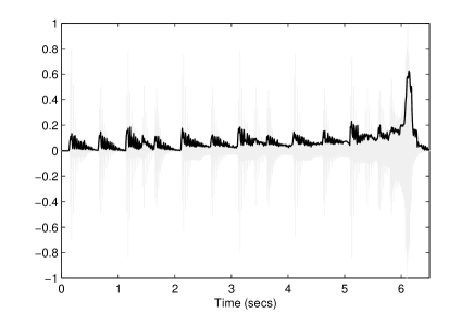
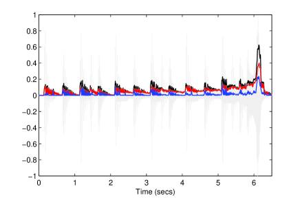
Since the Black_Hole_Billiards ring tone is a more complex signal, due to the superposition of the artificial sound, the information given by the local sparsity ratio is richer than in the previous cases. Notice for instance that the dark line in the left graph of Fig. 6 clearly indicates the offsets in the percussive part of the clip which has been superimposed to the GS chirp. Moreover this line, joining 512 points of inverse local sparsity ratio, also roughly follows the signal variation envelop. The graph on the right discriminates the local sparsity measure corresponding to atoms in the trigonometric component of the dictionary, and those in the dictionary $\mathcal{D}_{P}$. From bottom to top the first line (blue) represents the inverse local sparsity values corresponding to atoms in $\mathcal{D}_{P}$ and the next line (red) to atoms in $\mathcal{D}_{T}$. The top line (black) corresponds to atoms in the mixed dictionary $\mathcal{D}_{M}$ for facilitating the visual comparison. In this clip $20\%$ of atoms are from dictionary $\mathcal{D}_{P}$ and, as indicated by the blue line in the right graph of Fig. 6, a significant contribution of those atoms takes place within the blocks where the rapid rise of the GS tone takes place (c.f. spectrogram in Fig. 4).

4 Conclusions

We have here advanced an effective technique for the numerical representation of Gravitational Sound clips produced by the Laser Interferometer Gravitational-Wave Observatory (LIGO) and the Massachusetts Institute of Technology (MIT). Our technique is inscribed within the particular context of sparse representation and data reduction. We laid out a detailed procedure to this effect and were able to show that these types of signals can be approximated with high quality using significantly fewer elementary components than those required within the standard orthogonal basis framework.

Acknowledgments

Thanks are due to LIGO, MIT and Milde Science Communications for making available the GS tones we have used in this paper. We are particularly grateful to Prof. S. A. Hughes and Prof. B. Schutz, for giving us information on the generation of those signals.

References

- [1] J. L. Cervantes-Cota, S., Galindo-Uribarri, and G. F. Smoot, “A Brief History of Gravitational Waves”, Universe (2016) 2(3), 22; doi:10.3390/universe2030022.
- [2] A. Einstein, Über Gravitationswellen. In: Sitzungsberichte der Königlich Preussischen Akademie der Wis-senschaften Berlin (1918), 154–167.
- [3] B. P. Abbott et al. (LIGO Scientific Collaboration and Virgo Collaboration), Phys. Rev Lett. 116, 061102 (2016), DOI: 10.1103/PhysRevLett.116.061102
- [4] B. P. Abbott et al. (LIGO Scientific Collaboration and Virgo Collaboration) “Binary Black Hole Mergers in the First Advanced LIGO Observing Run”, Phys. Rev. X, 6, 041015, (2016)
- [5] B. P. Abbott et al. (LIGO Scientific Collaboration and Virgo Collaboration), “B. P. Abbott et al. (LIGO Scientific Collaboration and Virgo Collaboration), “Properties of the Binary Black Hole Merger GW150914”, Phys. Rev. Lett. 116, 241102 (2016), DOI: 10.1103/PhysRevLett.116.241102.
- [6] K. Belczynski, D. E. Holz, T Bulik, and R. O’Shaughnessy, “The first gravitational-wave source from the isolated evolution of two stars in the 40–100 solar mass range”, Nature, 534, 512–515 (2016) doi:10.1038/nature18322.
- [7] N. Yunes, K. Yagi, and F. Pretorius, “Theoretical physics implications of the binary black-hole mergers GW150914 and GW151226”, Phys. Rev. D, 94, 084002 (2016).
- [8] R. M. O’Leary, Y. Meiron, and B. Kocsis, “Dynamical formation signatures of black hole binaries in the first detected mergers by LIGO”, Astrophysical Journal Letters, 824, 1–L12 (2016).
- [9] S. S. Chen, D. L. Donoho, and M. A Saunders, “Atomic Decomposition by Basis Pursuit”, SIAM Journal on Scientific Computing, 20, 33–61 (1998).
- [10] S. Mallat and Z. Zhang, “Matching pursuit with time-frequency dictionaries,” IEEE Transactions on Signal Processing, 41, 3397–3415 (1993).
- [11] Y.C. Pati, R. Rezaiifar, and P.S. Krishnaprasad, “Orthogonal matching pursuit: recursive function approximation with applications to wavelet decomposition,” Proc. of the 27th ACSSC,1,40–44 (1993).
- [12] B. K. Natarajan, “Sparse Approximate Solutions to Linear Systems”, SIAM Journal on Computing, 24, 227–234 (1995).
- [13] L. Rebollo-Neira and D. Lowe, “Optimized orthogonal matching pursuit approach”, IEEE Signal Process. Letters, 9, 137–140 (2002)
- [14] M. Andrle, L. Rebollo-Neira, and E. Sagianos, “Backward-optimized orthogonal matching pursuit approach”, IEEE Signal Process. Let.,11,705–708 (2004).
- [15] J. A. Tropp, “Greed is good: algorithmic results for sparse approximation”, IEEE Transactions on Information Theory, 50, 2231–2242 (2004).
- [16] D. L. Donoho , Y. Tsaig , I. Drori , and J. Starck, “Stagewise Orthogonal Matching Pursuit”, IEEE Transactions on Information Theory, 58, 1094–1121 (2006).
- [17] D. Needell and J.A. Tropp, “CoSaMP: Iterative signal recovery from incomplete and inaccurate samples”, Applied and Computational Harmonic Analysis, 26, 301–321 (2009).
- [18] E. C. Smith, M. S. Lewicki, “Efficient auditory coding,” Nature , 439, no. 7079, pp. 978–982, 2006
- [19] J. Nam, J. Herrera, M. Slaney, and J. Smith, “Learning sparse feature representations for music annotation and retrieval,” in Proc. ISMIR , 2012.
- [20] D. L. Donoho, “Compressed sensing”, IEEE Trans. Inf. Theory,52, 1289–1306 (2006).
- [21] E. Candès and M. Wakin, “An introduction to compressive sampling”, IEEE Signal Processing Magazine, 25, 21 – 30 (2008).
- [22] R. Baraniuk, “More Is less: Signal processing and the data deluge”, Science, 331, 717 – 719 (2011).
- [23] http://http://www.eso.org/public/
- [24] http://hubblesite.org/
- [25] L. Rebollo-Neira, “Cooperative greedy pursuit strategies for sparse signal representation by partitioning”, Signal Processing, 125, 365–375 (2016).
- [26] L. Rebollo-Neira, G. Aggarwal, “A dedicated greedy pursuit algorithm for sparse spectral representation of music sound”, Journal of The Acoustic Society of America, 140 (2016).
- [27] L. Rebollo-Neira, J.Bowley Sparse representation of astronomical images, Journal of The Optical Society of America A, 30, 758–768 (2013).
- [28] http://www.nonlinear-approx.info/examples/node05.html
- [29] http://www.ligo.org/multimedia
- [30] http://gmunu.mit.edu/sounds/emri_sounds/a0.998/a0.998.html
- [31] S. A. Hughes, ‘The evolution of circular, non-equatorial orbits of Kerr black holes due to gravitational-wave emission”, Phys. Rev. D, 61, 084004 (2000); gr-qc/9910091.
- [32] S. A. Hughes, “Evolution of circular, non-equatorial orbits of Kerr black holes due to gravitational-wave emission: II. Inspiral trajectories and gravitational waveforms”, Phys. Rev. D, 64, 064004 (2001); gr-qc/0104041.
- [33] K. Glampedakis, S. A. Hughes, D. Kennefick, “Approximating the inspiral of test bodies into Kerr black holes”, Phys. Rev. D, 66, 064005 (2002); gr-qc/0205033.
- [34] S. A. Hughes, S. Drasco, E. E. Flanagan, J. Franklin, “Gravitational radiation reaction and inspiral waveforms in the adiabatic limit, Phys. Rev. Lett. 94, 221101 (2005); gr-qc/0504015.
- [35] S. Drasco and S. A. Hughes, “Gravitational wave snapshots of generic extreme mass ratio inspirals”, Phys. Rev. D, 73, (2006); gr-qc/0509101.