Revealing nonclassicality beyond Gaussian states via a single marginal distribution

Abstract

A standard method to obtain information on a quantum state is to measure marginal distributions along many different axes in phase space, which forms a basis of quantum state tomography. We theoretically propose and experimentally demonstrate a general framework to manifest nonclassicality by observing a single marginal distribution only, which provides a novel insight into nonclassicality and a practical applicability to various quantum systems. Our approach maps the 1-dim marginal distribution into a factorized 2-dim distribution by multiplying the measured distribution or the vacuum-state distribution along an orthogonal axis. The resulting fictitious Wigner function becomes unphysical only for a nonclassical state, thus the negativity of the corresponding density operator provides an evidence of nonclassicality. Furthermore, the negativity measured this way yields a lower bound for entanglement potential—a measure of entanglement generated using a nonclassical state with a beam splitter setting that is a prototypical model to produce continuous-variable (CV) entangled states. Our approach detects both Gaussian and non-Gaussian nonclassical states in a reliable and efficient manner. Remarkably, it works regardless of measurement axis for all non-Gaussian states in finite-dimensional Fock space of any size, also extending to infinite-dimensional states of experimental relevance for CV quantum informatics. We experimentally illustrate the power of our criterion for motional states of a trapped ion confirming their nonclassicality in a measurement-axis independent manner. We also address an extension of our approach combined with phase-shift operations, which leads to a stronger test of nonclassicality, i.e. detection of genuine non-Gaussianity under a CV measurement.

Nonclassicality is a fundamentally profound concept to identify quantum phenomena inaccessible from classical physics. It also provides a practically useful resource, e.g. entanglement, making possible a lot of applications in quantum information processing beyond classical counterparts ReviewCVQI ; Cerf ; ReviewGQI . A wide range of quantum systems, e.g. field amplitudes of light, collective spins of atomic ensembles, and motional modes of trapped ions, Bose-Einstein condensate and mechanical oscillators, can be employed for quantum information processing based on continuous variables (CVs) Cerf . It is of crucial importance to establish efficient and reliable criteria of nonclassicality for CV systems, desirably testable with less experimental resources, e.g. fewer measurement settings Richter2002 ; Richter2002' ; Mari2011 ; Park2015 ; ParkNha and with the capability of detecting a broad class of nonclassical states. In this paper, in view of the Glauber-Sudarshan P-function Glauber1963 ; Sudarshan1963 , those states that cannot be represented as a convex mixture of coherent states are referred to as nonclassical.

A standard method to obtain information on a CV quantum state is to measure marginal distributions along many different axes in phase space constituting quantum state tomography Lvovsky2009 . This tomographic reconstruction may reveal nonclassicality to some extent, e.g. negativity of Wigner function making only a subset of whole nonclassicality conditions. However it typically suffers from a legitimacy problem, i.e., the measured distributions do not yield a physical state when directly employed due to finite data and finite binning size D'Ariano1994 ; Lvovsky2009 . Much efforts was made to employ estimation methods finding a most probable quantum state closest to the obtained data Hradil1997 ; Banaszek1999 ; Rehacek2010 ; Teo2011 . There were also numerous studies to directly detect nonclassicality, e.g. an increasingly large number of hierarchical conditions Richter2002 requiring information on two or more marginal distributions or measurement of many higher-order moments Vogel ; Vogel' ; Bednorz . An exception would be the case of Gaussian states, with its nonclassical squeezing demonstrated by the variance of distribution along a squeezed axis.

Here we theoretically propose and experimentally demonstrate a simple, powerful, method to directly manifest nonclassicality by observing a single marginal distribution applicable to a wide range of nonclassical states. Our approach makes use of a phase-space map that transforms the marginal distribution (obtained from measurement) to a factorized Wigner distribution by multiplying the same distribution or the vacuum-state distribution along an orthogonal axis. We refer to those mathematical procedures as demarginalization maps (DMs), since a 1-dimensional marginal distribution is converted to a fictitious 2-dimensional Wigner function. The same method can be applied equally to the characteristic function as well as the Wigner function. We show that a classical state, i.e. a mixture of coherent states, must yield a physical state under our DMs. That is, the unphysicality emerging under DMs is a clear signature of nonclassicality. Remarkably, for all non-Gaussian states in finite dimensional space PN , our test works for an arbitrary single marginal distribution thus experimentally favorable. It also extends to non-Gaussian states in infinite dimension, particularly those without squeezing effect. We introduce a quantitative measure of nonclassicality using our DMs, which provides a lower bound of entanglement potential Asboth2005 —an entanglement measure under a beam-splitter setting versatile for CV entanglement generation Kim2002 ; Wang ; Asboth2005 ; Tahira2009 . Along this way, our method makes a rigorous connection between single-mode nonclassicality and negative partial transpose (NPT) entanglement Peres ; Horodecki ; Duan ; Simon ; MM ; MM' ; Walborn ; Walborn' ; Nha2008 ; Nha2012 , which bears on entanglement distillation EntanglementDistillation and nonlocality PeresConjecture ; PC1 ; PC2 ; PC3 ; PC4 ; PC5 ; PC6 ; PC7 .

As the measurement of a marginal distribution is highly efficient in various quantum systems, e.g. homodyne detection in quantum optics, our proposed approach can provide a practically useful and reliable tool in a wide range of investigations for CV quantum physics. We here experimentally illustrate the power of our approach by manifesting nonclassicality of motional states in a trapped-ion system. Specifically, we confirm the nonclassicality regardless of measured quadrature axis by introducing a simple faithful test using only a subset of data points, not requiring data manipulation under numerical methods unlike the case of state reconstruction. We also extend our approach combined with phase-randomization in order to obtain a criterion on genuine non-Gaussianity.

I Demarginalization maps and nonclassicality measure

I.1 Nonclassicality test via demarginalization maps

We first introduce our main tools, i.e. demarginalization maps (DMs),

$$\mathcal{D}_{1} :W_{\rho}(q,p)\mapsto M_{\rho}(x)M_{\rho}(y)\equiv W_{\rho}^{\rm DM1}(x,y),$$ (1)

$$\mathcal{D}_{2} :W_{\rho}(q,p)\mapsto M_{\rho}(x)M_{|0\rangle\langle 0|}(y)\equiv W_{\rho}^{\rm DM2}(x,y),$$ (2)

where $(x,y)^{T}=\mathcal{R}(\theta)(q,p)^{T}$ is a pair of orthogonal quadratures rotated from position $q$ and momentum $p$ with $\mathcal{R}(\theta)=\begin{pmatrix}\cos\theta&\sin\theta\\ -\sin\theta&\cos\theta\end{pmatrix}$. $M_{\rho}(x)=\int dyW_{\rho}(x,y)$ is a marginal distribution of the Wigner function $W_{\rho}(q,p)=\frac{2}{\pi}\mathrm{tr}[\rho\hat{D}(\alpha)(-1)^{\hat{n}}\hat{D}^{{\dagger}}(\alpha)]$, where $\hat{D}(\alpha)=e^{\alpha\hat{a}^{{\dagger}}-\alpha^{*}\hat{a}}$ is a displacement operator with $\alpha=q+ip$ Barnett ; Scully .

Our DM methods proceed as follows. Given a state with its Wigner function $W_{\rho}(q,p)$, we measure a marginal distribution $M_{\rho}(x)$ along a certain axis, $x=q\cos\theta+p\sin\theta$. We then construct a fictitious, factorized, Wigner function $W_{\rho}^{\rm DM}(x,y)$ either by replicating the obtained distribution as $M_{\rho}(x)M_{\rho}(y)$ (DM1) or by multiplying the marginal distribution of a vacuum state as $M_{\rho}(x)M_{|0\rangle\langle 0|}(y)$ (DM2), with $M_{|0\rangle\langle 0|}(y)=\sqrt{\frac{2}{\pi}}e^{-2y^{2}}$ (Fig. 1.). We test whether $W_{\rho}^{\rm DM}(x,y)$ is a legitimate Wigner function to represent a physical state.

Nonclassicality criteria—The constructed functions in Eqs. 1 and 2 are both in factorized forms, so judging their legitimacy is related to the problem what quantum states can possess a factorized Wigner function Note1 . Every coherent state $|\beta\rangle$ has a factorized Wigner function against all pairs of orthogonal quadratures, $W_{|\beta\rangle\langle\beta|}(x,y)=\frac{2}{\pi}e^{-2(x-\beta_{x})^{2}}e^{-2(y-\beta_{y})^{2}}$ Park2015 . Owing to this factorizability, the maps $\mathcal{D}_{1}$ and $\mathcal{D}_{2}$ transform a classical state into another classical one. A mixture of coherent states has a Wigner function

$$W_{\rho_{\mathrm{cl}}}(x,y)=\int d^{2}\beta P(\beta_{x},\beta_{y})W_{|\beta\rangle\langle\beta|}(x,y),$$ (3)

with the probability density $P(\beta_{x},\beta_{y})$ for a coherent state $|\beta\rangle$ ($\beta=\beta_{x}+i\beta_{y}$). Applying each DM leads to

$$\mathcal{D}_{j}[W_{\rho_{\mathrm{cl}}}(q,p)]=\int d^{2}\beta Q_{1}(\beta_{x})Q_{j}(\beta_{y})W_{|\beta\rangle\langle\beta|}(x,y)$$ (4)

$(j=1,2)$, where $Q_{1}(\beta_{x})=\int d\beta_{y}P(\beta_{x},\beta_{y})$ and $Q_{2}(\beta_{x})=\delta(\beta_{x})$ are nonnegative. The resulting distributions in Eq. 4 also represent a certain mixture of coherent states, hence a physical state. Therefore, if an unphysical Wigner function emerges under our DMs, the input state must be nonclassical.

Gaussian states—Let us first consider a Gaussian state $\sigma$ that has a squeezed quadrature $\hat{x}$ with $V_{x}\equiv\Delta^{2}\hat{x}<\frac{1}{4}$. Taking the squeezed marginal $M_{\sigma}(x)=\frac{1}{\sqrt{2\pi V_{x}}}e^{-\frac{(x-\langle\hat{x}\rangle)^{2}}{2V_{x}}}$ yields

$$\mathcal{D}_{1}[W_{\sigma}(q,p)] =\frac{1}{2\pi V_{x}}e^{-\frac{(x-\langle\hat{x}\rangle)^{2}}{2V_{x}}}e^{-\frac{(y-\langle\hat{x}\rangle)^{2}}{2V_{x}}},$$

$$\mathcal{D}_{2}[W_{\sigma}(q,p)] =\frac{1}{\pi\sqrt{V_{x}}}e^{-\frac{(x-\langle\hat{x}\rangle)^{2}}{2V_{x}}}e^{-2y^{2}},$$ (5)

both of which violate the uncertainty relation $\Delta\hat{x}\Delta\hat{y}\geq\frac{1}{4}$. Thus, the squeezed state turns into an unphysical state under our DMs. This method, of course, succeeds only when the observed marginal distribution is along a squeezed axis that generally extends to a finite range of angles, if not the whole angles supple . We can further make the test successful regardless of quadrature axis by introducing a random phase rotation on a Gaussian state supple . Note that a mixture of phase-rotations, which transforms a Gaussian to a non-Gaussian state, does not create nonclassicality, so the nonclassicality detected after phase rotations is attributed to that of the original state.

Non-Gaussian states—More importantly, we now address non-Gaussian states. Every finite-dimensional state (FDS) in Fock basis, i.e. $\rho=\sum_{j,k=0}^{N}\rho_{jk}|j\rangle\langle k|$ is nonclassical, since all coherent states (except vacuum), and their mixtures as well, have an extension to infinite Fock states. It is nontrivial to demonstrate the nonclassicality of FDS when one has access to limited information, e.g., a noisy state $f|0\rangle\langle 0|+(1-f)|1\rangle\langle 1|$ for $f\geq\frac{1}{2}$ has no simple signatures of nonclassicality like squeezing and negativity of Wigner function. We prove that our DMs are able to detect all non-Gaussian states in finite dimension of any size, with details in Sec. S4 of supple . The essence of our proof is that there always exists a submatrix of the density operator corresponding to DMs, which is not positive-definite. Remarkably, this non-positivity emerges for a marginal distribution along an arbitrary direction, which means that the nonclassicality of FDS is confirmed regardless of the quadrature axis measured, just like the phase-randomized Gaussian states introduced in supple . This makes our DM test experimentally favorable, while the degree of negativity may well depend on the quadrature axis except rotationally-symmetric states. Our criteria can further be extended to non-Gaussian states in infinite dimension, particularly those without squeezing effect supple .

As an illustration, we show the case of a FDS $|\Psi\rangle=\frac{1}{\sqrt{2}}\left(|0\rangle+|2\rangle\right)$, whose original Wigner function and matrix elements are displayed in Fig. 1 (a). Our DM methods yield matrix elements as shown in Fig. 1 (b) and (c). The non-positivity of the density operator is then demonstrated by, e.g., $\langle 0|\rho|0\rangle\langle 8|\rho|8\rangle-|\langle 0|\rho|8\rangle|^{2}<0$ under DM1 and $\langle 0|\rho|0\rangle\langle 4|\rho|4\rangle-|\langle 0|\rho|4\rangle|^{2}<0$ under DM2, respectively.

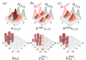
Figure 1: Illustrating DMs (a) original Wigner function $W_{\rho}(x,y)$ of $|\Psi\rangle=\frac{1}{\sqrt{2}}\left(|0\rangle+|2\rangle\right)$, with its marginal $M_{\rho}(x)=\int dyW_{\rho}(x,y)$ in the backdrop, (b) a fictitious Wigner function $W^{\rm DM1}(x,y)\equiv M_{\rho}(x)M_{\rho}(y)$, with the same distribution $M_{\rho}(y)$ replicated along the orthogonal axis (red solid curve), and (c) $W^{\rm DM2}(x,y)\equiv M_{\rho}(x)M_{|0\rangle\langle 0|}(y)$, with the vacuum-state distribution $M_{|0\rangle\langle 0|}(y)$ used (red solid curve). The second panels show the corresponding density matrix elements. $W^{\rm DM1}(x,y)$ and $W^{\rm DM2}(x,y)$ in (b) and (c) do not represent any physical states, confirming the nonclassicality of $|\Psi\rangle$.

I.2 Nonclassicality measure and entanglement potential

We may define a measure of nonclassicality using our DMs as

$$\mathcal{N}_{\mathrm{DM}}(\rho)\equiv\max_{\theta\in(0,\pi)}\frac{||\rho_{\mathrm{DM}}^{\theta}||_{1}-1}{2},$$ (6)

where $||\cdot||_{1}$ is a trace norm and $\rho_{\mathrm{DM}}^{\theta}$ a density matrix under DM using a marginal distribution at angle $\theta$. Our DM negativity possesses the following properties appropriate as a nonclassicality measure, with details in supple . (i) $\mathcal{N}_{\mathrm{DM}}=0$ for a classical state, (ii) convex, i.e. non-increasing via mixing states, $\mathcal{N}_{\mathrm{DM}}(\sum_{j}p_{j}\rho_{j})\leq\sum_{j}p_{j}\mathcal{N}_{\mathrm{DM}}(\rho_{j})$, and (iii) invariant under a classicality-preserving unitary operation, $\mathcal{N}_{\mathrm{DM}}(\hat{U}_{c}\rho\hat{U}_{c}^{{\dagger}})=\mathcal{N}_{\mathrm{DM}}(\rho)$, where $\hat{U}_{c}$ refers to displacement or phase rotation. Combining (ii) and (iii), we also deduce the property that (iv) $\mathcal{N}_{\mathrm{DM}}$ does not increase under generic classicality preserving operations (mixture of unitary operations).

Our nonclassicality measure also makes a significant connection to entanglement potential as follows. A prototypical scheme to generate a CV entangled state is to inject a single-mode nonclassical state into a beam splitter (BS) Kim2002 ; Wang ; Asboth2005 ; Tahira2009 . It is important to know the property of those entangled states under PT, which bears on the distillibility of the output to achieve higher entanglement. Our formalism makes a connection between nonclassicality of single-mode resources and NPT of output entangled states. The effect of PT in phase space is to change the sign of momentum, $W_{\rho_{12}}(q_{1},p_{1},q_{2},p_{2})\rightarrow W_{\rho_{12}}(q_{1},p_{1},q_{2},-p_{2})$. If the resulting Wigner function is unphysical, the state $\rho_{12}$ is NPT. We first show that all nonclassical states detected under our DMs can generate NPT entanglement via a BS setting.

We inject a single-mode state $\rho$ and its rotated version $\overline{\rho}=e^{i\frac{\pi}{2}\hat{n}}\rho e^{-i\frac{\pi}{2}\hat{n}}$ into a 50:50 beam splitter (BS), described as

$$W_{\rho}(q_{1},p_{1})W_{\overline{\rho}}(q_{2},p_{2})$$

$$\xrightarrow{\mathrm{BS}} W_{\rho}(\frac{q_{1}+q_{2}}{\sqrt{2}},\frac{p_{1}+p_{2}}{\sqrt{2}})W_{\overline{\rho}}(\frac{q_{1}-q_{2}}{\sqrt{2}},\frac{p_{1}-p_{2}}{\sqrt{2}}).$$ (7)

Applying PT on mode 2 and injecting the state again into a 50:50 BS, we have

$$W_{\rho}(\frac{q_{1}+q_{2}}{\sqrt{2}},\frac{p_{1}-p_{2}}{\sqrt{2}})W_{\overline{\rho}}(\frac{q_{1}-q_{2}}{\sqrt{2}},\frac{p_{1}+p_{2}}{\sqrt{2}})$$

$$\xrightarrow{\mathrm{BS}} W_{\rho}(q_{1},p_{2})W_{\overline{\rho}}(q_{2},p_{1})=W_{\rho}(q_{1},p_{2})W_{\rho}(p_{1},q_{2}).$$ (8)

Integrating over $q_{2}$ and $p_{2}$, the marginal Wigner function for mode 1 is given by $M_{\rho}(q_{1})M_{\rho}(p_{1})$, which is identical to DM1 of the state $\rho$ in Eq. 1. The other DM2 in Eq. 2 emerges when replacing the second input state $\overline{\rho}$ by a vacuum $\overline{\rho}=|0\rangle\langle 0|$. Therefore, if the original state $\rho$ is nonclassical under our DMs, the output entangled state via the BS scheme must be NPT.

In Ref. Asboth2005 , single-mode nonclassicality is characterized by entanglement potential via a BS setting, where a vacuum is used as an ancillary input to BS to generate entanglement. We may take negativity, instead of logarithmic negativity in Asboth2005 , as a measure of entanglement potential, i.e.,

$$\mathcal{P}_{\mathrm{ent}}[\rho]\equiv\frac{||[\hat{U}_{\mathrm{BS}}(\rho_{1}\otimes|0\rangle\langle 0|_{2})\hat{U}_{\mathrm{BS}}^{{\dagger}}]^{\mathrm{PT}}||_{1}-1}{2},$$ (9)

where $\hat{U}_{\mathrm{BS}}$ and $[\cdot]^{\mathrm{PT}}$ represent 50:50 beam-splitter operation and partial transpose on the mode 2, respectively. We then prove in supple that our DM2 measure provides a lower bound for the entanglement potential as

$$\mathcal{N}_{\mathrm{DM2}}[\rho]\leq\mathcal{P}_{\mathrm{ent}}[\rho].$$ (10)

Thus the nonclassicality measured under our framework indicates the degree of entanglement achievable via BS setting.

II Experiment

We experimentally illustrate the power of our approach by detecting nonclassicality of several motional states of a trapped ¹⁷¹Yb⁺ ion. For the manipulation of motional state, the single phonon-mode $\hat{a}$ along $\rm X$-direction in 3-dimensional harmonic potential with trap frequencies $\left(\omega_{\rm X},\omega_{\rm Y},\omega_{\rm Z}\right)=2\pi~{}(2.8,3.2,0.6)$ MHz is coupled to two internal levels of the $S_{1/2}$ ground state manifold, $|F=1,m_{F}=0\rangle\equiv|\uparrow\rangle$ and $|F=0,m_{F}=0\rangle\equiv|\downarrow\rangle$ with transition frequency $\omega_{\rm HF}=(2\pi)~{}12.642821$ GHz. We implement the anti-Jaynes-Cumming interaction $H_{\rm aJC}=\frac{\eta\Omega}{2}\hat{a}^{\dagger}\hat{\sigma}_{+}+{\rm h.c.}$ and the Jaynes-Cumming interaction $H_{\rm JC}=\frac{\eta\Omega}{2}\hat{a}\hat{\sigma}_{+}+{\rm h.c.}$ with $\sigma_{+}=|\uparrow\rangle\langle\downarrow|$. $H_{\rm aJC}$ is realized by two counter-propagating laser beams with beat frequency near $\omega_{\rm HF}+\omega_{\rm X}$ and $H_{\rm JC}$ with frequency near $\omega_{\rm HF}-\omega_{\rm X}$ Park2015 . $\eta=\Delta k\sqrt{\hbar/2M\omega_{\rm X}}$ is the Lamb-Dicke parameter, $\Omega$ the Rabi frequency of internal transition, $\Delta k$ the net wave-vector of the Raman laser beams and $M$ the ion mass.

For our test, we generate the Fock states $|n=1\rangle$ and $|n=2\rangle$, together with the ground state $|n=0\rangle$. First, we prepare the ground state by applying the standard Doppler cooling and the Raman sideband cooling. Then we produce the Fock states by a successive application of $\pi$-pulse of $H_{\rm aJC}$ transferring the state $|\downarrow,n\rangle$ to $|\uparrow,n+1\rangle$, and the $\pi$-pulse for internal state transition $|\uparrow,n+1\rangle$ to $|\downarrow,n+1\rangle$. We also generate a superposition state $\frac{1}{\sqrt{2}}(|0\rangle+|2\rangle)$ by applying the $\pi/2$ pulse of $H_{\rm aJC}$ and then the $\pi$ pulse of $H_{\rm JC}$.

Nonclassicality test— We measure a characteristic function $C_{\rho}(k_{\theta})\equiv\langle e^{-2ik\hat{x}_{\theta}}\rangle$ with $\hat{x}_{\theta}=\hat{x}\cos\theta+\hat{p}\sin\theta$, by first making the evolution $\hat{U}=e^{-ik\hat{x}_{\theta}\hat{\sigma}_{x}}$ (simultaneously applying $H_{\rm aJC}$ and $H_{\rm JC}$ with proper phases) and then measuring internal state $\hat{\sigma}_{z}=|\uparrow\rangle\langle\uparrow|-|\downarrow\rangle\langle\downarrow|$ at times $t_{i}$ ($k=\eta\Omega t$) Roos ; Roos' . Using $\hat{U}^{\dagger}\hat{\sigma}_{z}\hat{U}=\cos(2k\hat{x}_{\theta})\hat{\sigma}_{z}+\sin(2k\hat{x}_{\theta})\hat{\sigma}_{y}$, we obtain $\langle\cos(2k\hat{x}_{\theta})\rangle$ and $\langle\sin(2k\hat{x}_{\theta})\rangle$, with the internal state initially prepared in the eigenstates $|+\rangle_{z}$ and $|+\rangle_{y}$ of $\sigma_{z}$ and $\sigma_{y}$, respectively. The Fourier transform of $C_{\rho}(k_{\theta})$ gives the marginal distribution of $\hat{x}_{\theta}$ Roos ; Roos' . In contrast, we directly use it without the Fourier transform, for which our DMs work equally well as for the Wigner function. We test $C^{\rm DM1}\equiv C_{\rho}(k_{x})C_{\rho}(k_{y})$ or $C^{\rm DM2}\equiv C_{\rho}(k_{x})C_{|0\rangle\langle 0|}(k_{y})=C_{\rho}(k_{x})e^{-\frac{1}{2}\lambda_{k_{y}}^{2}}$, with its density operator $\rho=\frac{1}{\pi}\int dk_{x}dk_{y}C(k_{x},k_{y}){\hat{D}}^{{\dagger}}(k_{x},k_{y})$ unphysical for a nonclassical state.

To set a benchmark (noise level) for classical states, we prepared the motional ground state $|n=0\rangle$ and obtained its marginal distributions along six axes with 1000 repetitions for each time $t_{i}$. It yielded the negativity $\mathcal{N}_{\mathrm{DM2}}=0.019\pm 0.02$ as represented by gray shading in Fig. 2 supple . On the other hand, the Fock states $|n=1\rangle$ and $|n=2\rangle$ clearly manifest nonclassicality for each marginal distribution taken at three different angles $\theta$ in Fig. 2 (a), at much higher negativity with error bars considering a finite data 1000. To further show that our method works regardless of measured axis, we also tested a superposition state $\frac{1}{\sqrt{2}}(|0\rangle+|2\rangle)$ not rotationally symmetric in phase space. As shown in Fig. 2 (b), its nonclassicality is well demonstrated for all measured angles individually while the degree of negativity varies with the measured axis.

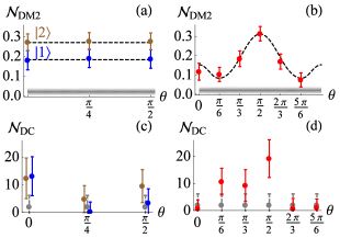
Figure 2: DM2 negativity against $\theta$ of the measured distribution $\langle e^{-2ik\hat{x}_{\theta}}\rangle$ for (a) Fock states $|1\rangle$ and $|2\rangle$ and (b) a superposition $\frac{1}{\sqrt{2}}(|0\rangle+|2\rangle)$ . Dashed: theoretical value, bullets with error bars: experiment, Grey shade: noise level for classical states. (c)-(d): Negativity under deconvolution test for Fock states $|1\rangle$ (blue), $|2\rangle$ (brown), and $\frac{1}{2}(|0\rangle+|2\rangle)$ (red), together with $|0\rangle$ (gray) using a $5\times 5$ moment-matrix.

Compared to our DM, one might look into nonclassicality directly via deconvolution, i.e. examining whether a marginal distribution $P(x)$ can be written as a sum of coherent-state distributions as $P(x)=\sqrt{\frac{2}{\pi}}\int d\tilde{x}\tilde{P}(\tilde{x})e^{-2(x-\tilde{x})^{2}}$, where $\tilde{P}(\tilde{x})$ must be positive-definite for classical states. $\tilde{P}(\tilde{x})$ is nothing but the marginal of Glauber-Sudarshan $P$-function, thus typically ill-behaved. One can test the positivity of $\tilde{P}(\tilde{x})$ alternatively using an $n\times n$ moment-matrix with elements $M_{ij}\equiv\langle\tilde{x}^{i+j}\rangle$ $(i,j=0,\dots,n-1)$Agarwal1993 . Figs. 2 (c) and (d) show the results under deconvolution using the same experimental data as we employed in Figs. 2 (a) and (b). To confirm nonclassicality, the degree of negativity must be large enough to beat that of the vacuum state including the statistical errors. Although those states produce negativity under deconvolution, their statistical errors are substantially overlapped with that of the vacuum state providing a much weaker evidence of nonclassicality than our DM. Full details are given in supple .

Instead of employing an entire characteristic function, we can also test our criterion by examining a subset of data using the Kastler-Loupias-Miracle-Sole (KLM) condition KLM ; KLM' ; KLM'' ; LegitimateW . This simple test provides a clear evidence of nonclassicality against experimental imperfections e.g. coarse-graining and finite data acquisition in other experimental platforms as well. The KLM condition states that the characteristic function $C_{\rho}(\xi)\equiv\mathrm{tr}[\rho\hat{D}(\xi)]$ for a legitimate quantum state must yield a $n\times n$ positive matrix $\mathcal{M}>0$ with matrix elements

$$\mathcal{M}_{jk}=C(\xi_{j}-\xi_{k})e^{\frac{1}{2}(\xi_{j}\xi_{k}^{*}-\xi_{j}^{*}\xi_{k})},$$ (11)

for an arbitrary set of complex variables $\{\xi_{1},\xi_{2},...,\xi_{n}\}$. In our case, we test the positivity of a matrix ($n=9$) constructed using $3\times 3$ points of rectangular lattice of size $d$ for the characteristic function under DM2 supple . As shown in Fig. 3 (a), the ground state $|0\rangle$ shows nonnegativity (thus the mixture of coherent states as well due to convexity of our method) for all values of $d$, whereas a nonclassical state $|\Psi\rangle=\frac{1}{\sqrt{2}}\left(|0\rangle+|2\rangle\right)$ manifests negativity in a certain range of $d$ confirming nonclassicality for each measured distribution at $\theta=\frac{\pi}{3},\frac{\pi}{2}$, and $\frac{2\pi}{3}$ (red solid curves) in Fig. 3 (b), (c) and (d), respectively. Furthermore, note that a mixture of the vacuum and the nonclassical state, $f|0\rangle\langle 0|+(1-f)|\Psi\rangle\langle\Psi|$ possesses a positive-definite Wigner function for $f\geq 0.66$, so even a full tomography may not directly show its nonclassicality via negativity. In contrast, our simple method manifests nonclassicality for $f=0.66$, as shown by blue dashed curves in Fig. 3 (b), (c) and (d). For Fock states, we consider the matrix test using $5\times 5$ lattice-points, which confirms negativity at the mixing $f=0.5$ with vacuum giving a non-negative Wigner function for both states $|1\rangle$ and $|2\rangle$ in Fig. 3 (e) and (f).

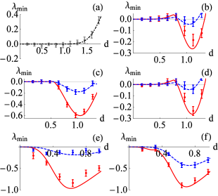
Figure 3: KLM test under DM2 using a matrix of $3\times 3$ (a-d) and $5\times 5$ (e,f) lattice points, respectively, with $\lambda_{\rm min}$ the lowest eigenvalue for each lattice size $d$ supple . Negative $\lambda_{\rm min}$ manifests the nonclassicality of the considered state. Solid (pure-state $|\Psi\rangle$) and dashed (mixed-state $f|0\rangle\langle 0|+(1-f)|\Psi\rangle\langle\Psi|$) curves represent theoretical predictions while bullets with error bars represent experimental data. (a) motional ground state $|0\rangle$, (b-d) $|\Psi\rangle=\frac{1}{\sqrt{2}}\left(|0\rangle+|2\rangle\right)$ for the measured angles at $\theta=\frac{\pi}{3},\frac{\pi}{2}$, and $\frac{2\pi}{3}$, respectively, (e) Fock state $|1\rangle$ and (f) Fock state $|2\rangle$. For mixed states (dashed curves), we use $f=0.66$ in (b-d) and $f=0.5$ in (e,f), respectively.

Genuine non-Gaussianity—We further extend our approach combined with phase-randomization to derive a criterion on genuine non-Gaussianity. Notably there exist quantum tasks that cannot be achieved by Gaussian resources, e.g. universal quantum computation Lloyd , CV nonlocality test NhaCV ; NhaCV' , entanglement distillation Eisert ; Fiurasek ; Giedke and error correction Niset . It is a topic of growing interest to detect genuine non-Gaussianity that cannot be addressed by a mixture of Gaussian states. Previous approaches all address particle nature like the photon-number distribution Filip2014 ; Jezek ; Straka2014 and the number parity in phase space Park2015 ; Genoni2013 ; Hughes2014 for this purpose. Here we propose a method to examine a genuinely CV characteristics of marginal distributions. Our criterion can be particularly useful to test a class of non-Gaussian states diagonal in the Fock basis, $\rho=\sum p_{n}|n\rangle\langle n|$, thus rotationally symmetric in phase space. For this class, one may detect nonclassicality using photon-number moments Vogel' , which can be experimentally addressed efficiently by phase-averaged quadrature measurements Munroe1995 ; Banaszek1997 . Lvovsky and Shapiro experimentally demonstrated the nonclassicality of a noisy single-photon state $f|0\rangle\langle 0|+(1-f)|1\rangle\langle 1|$ for an arbitrary $f$ Shapiro using the Vogel criterion Vogel'' . In contrast, we look into the genuine non-Gaussianity of non-Gaussian states as follows.

For a Gaussian state $\rho_{\rm G}$, the phase-randomization gives $\sigma\equiv\frac{1}{N}\sum_{k=0}^{N-1}e^{-i\theta_{k}{\hat{n}}}\rho_{\rm G}e^{i\theta_{k}{\hat{n}}}$ with $\theta_{k}\equiv\frac{k}{N}\pi$. As the number $N$ of phase rotation grows, the DM negativity of Gaussian states decreases. With $N\rightarrow\infty$ (full phase randomization), we obtain the Gaussian bound $\mathcal{B}_{\rm G}\approx 0.0887$ supple . Thus, if a state manifests a larger DM negativity as $\mathcal{N}>\mathcal{B}_{\rm G}$, it confirms genuine non-Gaussianity. We plot the Gaussian bounds for finite rotations $N=6$ and $N=12$ with $\mathcal{B}_{\rm G}\approx 0.0887$ against energy $n$ in Fig. 4. Our data for the state $|2\rangle$, which shows negativity insensitive to measured angles in Fig. 2, indicates genuine non-Gaussianity for the mixed states $f|0\rangle\langle 0|+(1-f)|2\rangle\langle 2|$ with $f=1-\frac{n}{2}$. For example, the $N=12$ case (brown dot-dashed) as well as the full phase randomization (black dashed horizontal) confirms quantum non-Gaussianity at $f=\frac{1}{2}$ corresponding to a positive Wigner-function.

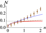
Figure 4: DM negativity of $f|0\rangle\langle 0|+(1-f)|2\rangle\langle 2|$ (bullet with error bar) from experimental data. Maximum Gausssian negativity under $N=6$ (blue dotted), $N=12$ (brown dot-dashed) and $N\rightarrow\infty$ (black dashed horizontal) phase rotations is given against energy $n$, the negativity above which confirms genuine non-Gaussianity.

III Conclusion and Remarks

Measuring marginal distributions along different axes in phase space forms a basis of quantum-state tomography with a wide range of applications. A marginal distribution is readily obtained in many different experimental platforms, e.g. by an efficient homodyne detection in quantum optical systems Lvovsky2009 ; Lvovsky2001 ; Ourjoumtsev2006 ; Huisman2009 ; Cooper2013 and by other quadrature measurements in trapped ion Roos ; Roos' ; ion , atomic ensembles as , optomechanics opto ; opto' , and circuit QED systems CQED ; CQED' . We here demonstrated that only a single marginal distribution can manifest nonclassicality by employing our demarginalization maps (DMs). Our DM methods are powerful to detect a wide range of nonclassical states, particularly non-Gaussian states. They provide a practical merit with less experimental efforts and make a stronger test of nonclassicality by analyzing data without numerical manipulation unlike state tomography.

Remarkably, nonclassicality can be demonstrated regardless of measured quadrature axis for all FDS states, which was also experimentally confirmed using a trapped ion system. We clearly showed that the proposed method provides a reliable nonclassicality test directly using a finite number of data, which can be further extended to other CV systems. In addition to the KLM test used here, we can manifest nonclassicality by looking into single marginal distributions under other forms, e.g. functional Nha2012 and entropic EUR ; EUR' inequalities. We also extended our approach to introduce a criterion on genuine non-Gaussianity employing marginal distributions combined with phase-randomization process. Our nonclassicality and non-Gaussianity tests were experimentally shown to successfully detect non-Gaussian states even with positive-definite Wigner functions whose nonclassicality is thus not immediately evident by the tomographic construction of Wigner function. As a note, for those nonclassical states with positive Wigner functions, one may use generalized quasi probability distributions like a filtered P-function Agarwal1970-1 ; Agarwal1970-2 ; Agarwal1970-3 . For example, the experiment in Kiesel2011 introduced a nonclassicality filter to construct a generalized P-function that yields a regularized distribution with negativity as a signature of nonclassicality for the case of photon-added thermal states. On the other hand, our DM method does not require a tomographic construction and provides a faithful test reliable against experimental imperfections like finite data and coarse graining.

Moreover, we established the connection between single-mode nonclassicality and NPT entanglement via BS setting—a prototypical model of producing CV entanglement. The negativity under our DM framework provides a quantitative measure of useful resource by identifying the minimum level of entanglement achievable in Eq. 10 NN . Nonclassicality and non-Gaussianity are important resources making a lot of quantum tasks possible far beyond classical counterparts. We thus hope our proposed method could provide a valuable experimental tool and a novel fundamental insight for future studies of CV quantum physics by critically addressing them.

Acknowledgements— M.S.Z. and H.N. were supported by National Priorities Research Program Grant 8-751-1-157 from the Qatar National Research Fund and K.K. by the National Key Research and Development Program of China under Grants 2016YFA0301900 and 2016YFA0301901 and the National Natural Science Foundation of China under Grants 11374178 and 11574002.

Supplemental Information

S1. Experiment: Analysis of fictitious characteristic function

We here explain how our experimental data are analyzed to yield a quantitative measure of DM negativity for each state in Fig. 2 and the lowest eigenvalue of KLM test in Fig. 3 of main text.

• DM2 negativity

First, to determine the DM negativity (noise level) of classical states, we prepared the motional ground state $|0\rangle$ and observed the marginal distributions $C(k_{x_{\theta}})\equiv\langle e^{-2ik\hat{x}_{\theta}}\rangle$, where $\hat{x}_{\theta}=\hat{x}\cos\theta+\hat{p}\sin\theta$, over six different angles $\theta$ with 1000 data at each time $t_{i}$ with $k=\eta\Omega t_{i}$. The resulting distribution including all data with error bars at each $k_{x}$ is drawn in Fig. 5 (a). A fictitious characteristic function is then constructed under DM2 as $C(k_{x},k_{y})=C(k_{x})e^{-\frac{1}{2}k_{y}^{2}}$, of which contour plot is given in Fig. 5 (c). We calculate the negativity of the corresponding density operator $\rho=\frac{1}{\pi}\int dk_{x}dk_{y}C(k_{x},k_{y}){\hat{D}}^{{\dagger}}(k_{x},k_{y})$ in the number-state basis. In Fig. 5 (e), we show the matrix elements $\rho_{mn}^{\rm DM2}$ of the density operator. $\frac{||\rho^{\mathrm{DM2}}||_{1}-1}{2}$ gives the result $\mathcal{N}_{\mathrm{DM2}}=0.019\pm 0.02$ in the main text.

On the other hand, for the case of a nonclassical state, e.g. $\frac{1}{\sqrt{2}}(|0\rangle+|2\rangle)$, the same procedures are taken for each measured axis, of which result, e.g. at $\theta=\frac{\pi}{2}$, is displayed in Fig. 5 (b,d,f).

• KLM test

For the purpose of KLM test mentioned in the main text, we choose a matrix using $n\times n$ lattice points in the space of characteristic function. For example, we illustrate the case of $3\times 3$ square lattice (black dots) in Figs.  5 (c) and (d). We may look at matrices by changing the lattice size $d$ according to data availability, all of which must give nonnegative eigenvalues for classical states. In other words, if there exists a negative $\lambda_{\rm min}$ for any $d$, it confirms nonclassicality.

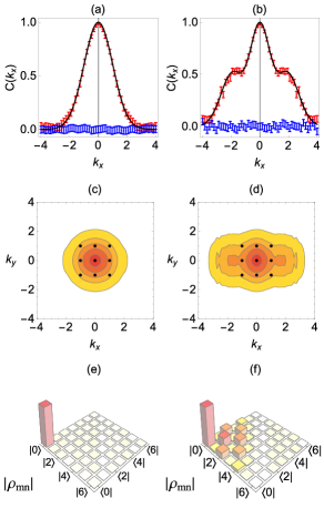
Figure 5: A marginal distribution $C(k_{x})$ of characteristic function for (a) ground state $|0\rangle$ and (b) superposition state $\frac{1}{\sqrt{2}}(|0\rangle+|2\rangle)$. Black solid curves represent theoretical predictions while red and blue dots represent the real and the imaginary parts of experimental data with error bars. (c), (d) Contour plots of fictitious characteristic function $C(k_{x},k_{y})=C(k_{x})e^{-\frac{1}{2}k_{y}^{2}}$. (e), (f) matrix elements $\rho_{mn}^{\rm DM2}$ of the corresponding density operators.

S2. Comparison of DM and deconvolution

Given a marginal distribution, one can also look into nonclassicality via a deconvolution method instead of our DM. That is, one examines whether the obtained probability distribution $P(x)$ can be written as a convex sum of coherent-state distributions as $P(x)=\sqrt{\frac{2}{\pi}}\int d\tilde{x}\tilde{P}(\tilde{x})e^{-2(x-\tilde{x})^{2}}$, where $\tilde{P}(\tilde{x})$ must be positive-definite for classical states. In other words, if one finds negativity of $\tilde{P}(\tilde{x})$ under a Gaussian deconvolution of $P(x)$, it is a signature of nonclassicality. For their corresponding characteristic functions $C(k)=\int dxP(x)e^{-2ikx}$ and ${\tilde{C}}(k)=\int d\tilde{x}\tilde{P}(\tilde{x})e^{-2ik\tilde{x}}$, respectively, the deconvolution gives the relation ${\tilde{C}}(k)=C(k)e^{\frac{1}{2}k^{2}}$.

First, note that $\tilde{P}(\tilde{x})$ is nothing but the marginal distribution of Glauber-Sudarshan $P$-function, thus it is usually ill-behaved, e.g. delta-function for a coherent state and singular for Fock states. However, one can test the positivity of $\tilde{P}(\tilde{x})$ alternatively based on a moment test. For a classical state, a $n\times n$ matrix whose elements are given by $M_{ij}\equiv\langle\tilde{x}^{i+j}\rangle$ $(i,j=0,\dots,n-1)$ must be positive-definite at all levels of $n$. The moments $\langle\tilde{x}^{m}\rangle$ can be obtained via the moments $\langle x^{m}\rangle$ of the regular probability distribution $P(x)$ by way of $\langle\tilde{x}^{m}\rangle=2^{-3m/2}\langle H_{m}(\sqrt{2}x)\rangle$ with $H_{m}(x)$ the Hermite polynomial of order $m$. To derive it, let us use a method of operator ordering as follows. Due to the Baker–Campbell–Hausdorff formula, we have $e^{\lambda(\hat{a}+\hat{a}^{{\dagger}})}=e^{\lambda^{2}/2}e^{\lambda\hat{a}^{{\dagger}}}e^{\lambda\hat{a}}$, i.e. $:e^{\lambda(\hat{a}+\hat{a}^{{\dagger}})}:=e^{\lambda\hat{a}^{{\dagger}}}e^{\lambda\hat{a}}=e^{-\lambda^{2}/2}e^{\lambda(\hat{a}+\hat{a}^{{\dagger}})}$. We then obtain

$$:(\hat{a}+\hat{a}^{{\dagger}})^{m}:=\lim_{\lambda\rightarrow 0}\frac{\partial^{m}}{\partial\lambda^{m}}:e^{\lambda(\hat{a}+\hat{a}^{{\dagger}})}:$$

$$=\lim_{\lambda\rightarrow 0}\frac{\partial^{n}}{\partial\lambda^{m}}e^{-\lambda^{2}/2}e^{\lambda(\hat{a}+\hat{a}^{{\dagger}})}$$

$$=\lim_{\lambda\rightarrow 0}\sum_{k=0}^{m}\binom{m}{k}\frac{\partial^{k}}{\partial\lambda^{k}}e^{-\lambda^{2}/2}\frac{\partial^{m-k}}{\partial\lambda^{m-k}}e^{\lambda(\hat{a}+\hat{a}^{{\dagger}})}$$

$$=\lim_{\lambda\rightarrow 0}\sum_{k=0}^{m}\binom{m}{k}2^{-k/2}e^{-\lambda^{2}/2}H_{k}(-\lambda/\sqrt{2})(\hat{a}+\hat{a}^{{\dagger}})^{m-k}e^{\lambda(\hat{a}+\hat{a}^{{\dagger}})}$$

$$=2^{-m/2}\sum_{k=0}^{m}\binom{m}{k}H_{k}(0)\{\sqrt{2}(\hat{a}+\hat{a}^{{\dagger}})\}^{m-k}$$

$$=2^{-m/2}H_{m}\bigg{(}\frac{\hat{a}+\hat{a}^{{\dagger}}}{\sqrt{2}}\bigg{)},$$ (12)

which yields the desired relation $:\hat{q}^{m}:=2^{-3m/2}H_{m}(\sqrt{2}\hat{q})$ with $\hat{q}=\frac{\hat{a}+\hat{a}^{{\dagger}}}{2}$. Note that we have used $H_{m}(x)=(-1)^{m}e^{x^{2}}\frac{d^{m}}{dx^{m}}e^{-x^{2}}$, $H_{m}(-x)=(-1)^{m}H_{m}(x)$ and $H_{m}(x+y)=\sum_{k=0}^{m}\binom{m}{k}H_{k}(x)(2y)^{m-k}$.

For a fair comparison with our DM, we here show the results of moment-matrix test under deconvolution for the states $|1\rangle$, $|2\rangle$ and $\frac{1}{\sqrt{2}}(|0\rangle+|2\rangle)$ together with the vacuum $|0\rangle$ using the same experimental data as we employed in Fig. 2 of the main text. To confirm nonclassicality, the degree of negativity must be large enough to beat that of the vacuum state including the statistical errors. As shown in Fig. 6, those nonclassical states produce negativity under deconvolution, however their statistical errors are substantially overlapped with that of the vacuum state making the interpretation weak (with the only exception at $\theta=\frac{\pi}{2}$ for the state $\frac{1}{\sqrt{2}}(|0\rangle+|2\rangle)$). This is clearly contrasted with the results under our DM in Fig. 2 of the main text.

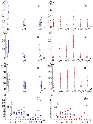
Figure 6: (a)-(f) Negativity under deconvolution method with error bars for the same experimental data used in Fig. 2 of the main text. Left column: Fock states $|1\rangle$ (blue), $|2\rangle$ (brown), Right column: superposition state $\frac{1}{\sqrt{2}}(|0\rangle+|2\rangle)$ (red), together with $|0\rangle$ (gray) against measurement angle $\theta$. The size of the moment-matrix considered increases as $3\times 3$ (a,b), $5\times 5$ (c,d) and $7\times 7$ (e,f), respectively. (g,h) Behavior of statistical error $\Delta_{m}$ of the moment $\langle\tilde{x}^{m}\rangle$ with a finite data $N=1000$ for (g) the Fock states $|1\rangle$ (blue), $|2\rangle$ (brown) and (h) the superposition $\frac{1}{\sqrt{2}}(|0\rangle+|2\rangle)$ (red) together with $|0\rangle$ (gray). Inset: magnified view for a small $m$.

One may try to optimize the matrix test by increasing the size $n$ of the matrix. This is theoretically valid, since the negativity not appearing in a low-dimension matrix can be found in a higher-dimension matrix as the latter encompasses the former. However, under practical situations with a finite number $N$ of data, the statistical error of the moment $\langle\tilde{x}^{m}\rangle$ given by $\Delta_{m}=\frac{2^{-3m/2}}{\sqrt{N}}\sqrt{\langle H_{m}^{2}(\sqrt{2}x)\rangle-\langle H_{m}(\sqrt{2}x)\rangle^{2}}$ exponentially increase with $m$. For instance, $\Delta_{m}=\sqrt{m!4^{-m}/N}$ for the vacuum state whereas it grows at a higher rate for typical nonclassical states as shown in Fig. 6 (g) and (h). It is thus harder with a larger $m$ to beat the reference level (vacuum) of nonclassicality with significant errors, and the matrix test becomes optimized at a moderate level of matrix dimension. As shown in Fig. 6, the test does not necessarily improve by increasing the matrix size. If one obtains much more data $N$, the effect of statistical error may be reduced, however, the fact that our DM method works well already with a low number of data is an evidence of superioity in manifesting nonclassicality. Note that our DM method employs well-behaved square-integrable functions by its construction unlike the deconvolution method. Furthermore, unlike the deconvolution method aiming only at detecting nonclassicality, our DM formalism also constitute a useful framework to connect nonclassicality and quantum entanglement in CV setting and to address a genuine non-Gaussianity of CV systems that has been of growing interest.

S3. Testing Gaussian states under DMs

As stated in the main text, a Gaussian nonclassical state, i.e. squeezed state, can be detected under our DMs if the measured marginal distribution is along a squeezed axis. For a given Gaussian state, we first determine a success range of measurement angles to manifest its nonclassicality. We later show that the nonclassicality can be demonstrated regardless of measurement axis by converting the Gaussian state to a non-Gaussian state under a finite number of phase rotations, which does not create nonclassicality.

A single-mode Gaussian state can generally be represented as a displaced squeezed thermal state,

$$\sigma=\hat{D}(\alpha)\hat{S}(r,\phi)\sigma_{\mathrm{th}}(\bar{n})\hat{S}^{{\dagger}}(r,\phi)\hat{D}^{{\dagger}}(\alpha),$$ (13)

where $\hat{S}(r,\phi)=\exp[-\frac{r}{2}(e^{2i\phi}\hat{a}^{{\dagger}2}-e^{-2i\phi}\hat{a}^{2})]$ is a squeezing operator ($r$: squeezing strength, $\phi$: squeezing direction), and $\sigma_{\mathrm{th}}(\bar{n})=\sum_{n=0}^{\infty}\frac{\bar{n}^{n}}{(\bar{n}+1)^{n+1}}|n\rangle\langle n|$ is a thermal state with mean photon number $\bar{n}$. The displacement does not affect the physicality issue under our DM methods, so we may set $\alpha=0$ without loss of generality. Then a Wigner function with $\phi=0$ (squeezed along $q$-axis) is given by

$$W_{\sigma}(q,p)=\frac{2\mu}{\pi}\exp[-2\mu(e^{2r}q^{2}+e^{-2r}p^{2})],$$ (14)

with $\mu=\frac{1}{1+2\bar{n}}$ the purity of the state. Its marginal distribution along the direction $\theta$ rotated from position $q$ is obtained as

$$M_{\sigma}(x)=\frac{1}{\sqrt{2\pi V_{\theta}}}\exp\bigg{(}-\frac{x^{2}}{2V_{\theta}}\bigg{)},$$ (15)

where $V_{\theta}=\frac{1}{4\mu}(\cosh 2r-\cos 2\theta\sinh 2r)$ is the variance. We identify the squeezing range $V_{\theta}<\frac{1}{4}$ to be $|\theta|<\frac{1}{2}\arccos\frac{\cosh 2r-\mu}{\sinh 2r}\equiv|\theta|_{\mathrm{sq}}$. We thus obtain a success probability $\eta_{\mathrm{sq}}$ that a randomly chosen angle $\theta\in[0,\frac{\pi}{2}]$ for a marginal distribution can detect nonclassicality as

$$\eta_{\mathrm{sq}}=\frac{|\theta|_{\mathrm{sq}}}{\frac{\pi}{2}}=\frac{1}{\pi}\arccos\frac{\cosh 2r-\mu}{\sinh 2r}.$$ (16)

We plot $\eta_{\mathrm{sq}}$ as a function of the purtiy $\mu\equiv\mathrm{tr}\rho^{2}$ and squeezing strength $r$ in Fig. 7. In general, $\eta_{\mathrm{sq}}$ monotonically increases with the purity $\mu$. On the other hand, it decreases with $r$ as the range of squeezed quadratures decreases with the degree of squeezing. For instance, in the extreme squeezing $r\rightarrow\infty$, the range of squeezing direction becomes $|\theta|_{\mathrm{sq}}\rightarrow 0$.

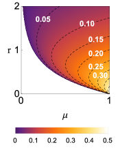
Figure 7: Contour for the probability of detecting nonclassicality for a Gaussian state with an unknown squeezing direction, i.e., $\eta_{\mathrm{sq}}$ in Eq. (16), against purity $\mu$ and squeezing $r$.

• Detecting Gaussian states under a classicality-preserving operation

We now introduce a finite number of phase rotations, which does not create nonclassicality, and show that it enables us to detect the nonclassicality of a Gaussian state regardless of measurement axis. The phase-randomizing operation generally transforms a Gaussian state to a non-Gaussian state and it was employed, e.g., for the distillation of squeezing Franzen and the reconstruction of a Wigner function of rotationally-symmetric state (Fock states) Grangier . We here use our DM2 approach and give proof in two-steps: (i) DM2 detects every nonclassical marginal distribution. (ii) The marginal distribution obtained from a squeezed state under phase-randomization is always nonclassical.

(i) Connection between DM2 and the Hamburger moment problem

For a given state $\rho$, DM2 gives the Wigner function as

$$W_{\mathcal{D}_{2}[\rho]}(q,p)=M_{\rho}(q)\sqrt{\frac{2}{\pi}}e^{-2p^{2}},$$ (17)

which is equivalent to the Glauber-P representation as

$$\mathcal{D}_{2}[\rho]=\int_{-\infty}^{\infty}dxT_{\rho}(x)|x\rangle\langle x|.$$ (18)

Here $\ket{x}$ represents a coherent state with real amplitude $x$ and the quasi-probability density $T_{\rho}(x)$ connects to the marginal distribution by $M_{\rho}(q)=\int_{-\infty}^{\infty}T_{\rho}(x)\sqrt{\frac{2}{\pi}}e^{-2(q-x)^{2}}$. (Note that $\mathcal{D}_{2}[\rho]$ is classical if and only if $T_{\rho}(x)$ is non-negative. We thus see that if the marginal distribution $M_{\rho}(q)$ cannot be expressed as a positive sum of normal distributions with $\sigma=\frac{1}{2}$ (vacuum fluctuation), the corresponding $\mathcal{D}_{2}[\rho]$ cannot represent a classical state.)

In addition, the density operator $\mathcal{D}_{2}[\rho]$ is unphysical if and only if there exists a pure state $\ket{\psi}=\sum_{n}c_{n}\ket{n}$ satisfying

$$\bra{\psi}\mathcal{D}_{2}[\rho]\ket{\psi} =\sum_{n=0}^{\infty}\sum_{m=0}^{\infty}c_{n}^{*}c_{m}\int_{-\infty}^{\infty}dxT_{\rho}(x)\braket{n}{x}\braket{x}{m}$$

$$=\sum_{n=0}^{\infty}\sum_{m=0}^{\infty}\frac{c_{n}^{*}}{\sqrt{n!}}\frac{c_{m}}{\sqrt{m!}}\int_{-\infty}^{\infty}dxT_{\rho}(x)e^{-x^{2}}x^{n+m}$$

$$<0.$$ (19)

In measure theory, it is known that for the moments $a_{n}=\int_{-\infty}^{\infty}x^{n}d\rho(x)$, the measure $\rho$ is positive if and only if

$$\sum_{n=0}^{N}\sum_{m=0}^{N}\beta_{n}^{*}\beta_{m}a_{n+m}\geq 0,$$ (20)

is satisfied for every non-negative integer $N$ and every set of complex variables $\{\beta_{0},...,\beta_{N}\}$ (Hamburger moment problem) ReedSimon . Comparing Eqs. (19) and (20), we see that $\mathcal{D}_{2}[\rho]$ is unphysical if and only if $T_{\rho}(x)$ fails to be positive. It therefore proves that $\mathcal{D}_{2}[\rho]$ becomes unphysical for every nonclassical marginal distribution.

(ii) Gaussian states under a finite number of phase rotations

For a general Gaussian state in Eq. (13), we apply $N$ (finite) phase rotations of angles $\{0,\frac{1}{N}\pi,...,\frac{N-1}{N}\pi\}$ with $N\geq\lceil\frac{1}{\eta_{\mathrm{sq}}}\rceil$, where $\eta_{\mathrm{sq}}$ is given in Eq. (16). An equal mixture of those rotations gives a marginal distribution

$$M_{\rho}(x)=\frac{1}{N}\sum_{k=0}^{N-1}\frac{1}{\sqrt{2\pi v_{k}}}e^{-\frac{x^{2}}{2v_{k}}},$$ (21)

with $v_{k}=\frac{1}{4\mu}[\cosh 2r-\cos 2(\theta+\frac{k}{N}\pi)\sinh 2r]$. Importantly, there always exists a set of $k$ satisfying $v_{k}<\frac{1}{4}$ (squeezing) regardless of $\theta$ (measured axis), whenever $N\geq\lceil\frac{1}{\eta_{\mathrm{sq}}}\rceil$ is satisfied. Below we show that the distribution in Eq. (21) cannot be represented as a mixture of Gaussian distributions all with vacuum noise. Together with the property (i), this proves that the resulting non-Gaussian state can be detected regardless of quadrature axis under DM2 method.

Suppose that $M_{\rho}(x)$ in Eq. (21) be written as a mixture of coherent-state distributions, i.e.

$$M_{\rho}(x)=\frac{1}{N}\sum_{k=0}^{N-1}\frac{1}{\sqrt{2\pi v_{k}}}e^{-\frac{x^{2}}{2v_{k}}}=\sum_{k^{\prime}}\frac{p_{k^{\prime}}}{\sqrt{\pi/2}}e^{-2(x-x_{k^{\prime}})^{2}},$$

then one encounters a contradiction. Let us take a Fourier transform, $\int dxe^{-ixy}M_{\rho}(x)$, and then multiply both sides by $e^{\frac{v}{2}y^{2}}$ with $v\equiv{\rm min}\{v_{k}\}<\frac{1}{4}$. It gives

$$\frac{1}{N}+\frac{1}{N}\sum_{k\neq k_{\rm min}}e^{-\frac{1}{2}(v_{k}-v)y^{2}}=\sum_{k^{\prime}}p_{k^{\prime}}e^{-ix_{k^{\prime}}y}e^{-\frac{1}{2}(\frac{1}{4}-v)y^{2}},$$

where the sum in the LHS excludes the terms with $v_{k}=v={\rm min}\{v_{k}\}$. It is readily seen that Eq. (23) cannot be satisfied at all $y$, e.g., LHS=$\frac{1}{N}$ and RHS=0 as $y\rightarrow\infty$.

• Gaussian bound under phase randomization

Let us now consider how the degree of nonclassicality (DM negativity) is bounded for all Gaussian states by a full phase-randomization. When the measured quadrature distribution is Gaussian with variance $V$, the Wigner function under DM2 is given by

$$W_{\sigma}^{\mathrm{DM2}}(x,y)=\frac{1}{\pi\sqrt{V}}\exp\bigg{(}-\frac{x^{2}}{2V}-2y^{2}\bigg{)},$$ (24)

and the corresponding density matrix by

$$\sigma^{\prime}=\sum_{n=0}^{\infty}\lambda_{n}\hat{S}(r,\frac{\pi}{2})|n\rangle\langle n|\hat{S}^{{\dagger}}(r,\frac{\pi}{2}),$$ (25)

where $r=-\frac{1}{2}\log 2\sqrt{V}$ and $\lambda_{n}=\frac{2}{2\sqrt{V}+1}(\frac{2\sqrt{V}-1}{2\sqrt{V}+1})^{n}$ represent the eigenvalues of $\sigma^{\prime}$. A direct calculation gives its DM negativity as

$$N_{\mathrm{DM2}}(V)=\max\bigg{(}\frac{1}{4\sqrt{V}}-\frac{1}{2},0\bigg{)}.$$ (26)

Using the convexity of the DM negativity (proved in the next section), we deduce that the DM negativity of a squeezed state $\rho_{\rm G}$ under phase randomization, i.e. $\sigma\equiv\frac{1}{2\pi}\int_{0}^{2\pi}d\theta e^{-i\theta{\hat{n}}}\rho_{\rm G}e^{i\theta{\hat{n}}}$ must be bounded as

$$\mathcal{N}_{\mathcal{D}[\sigma]} \leq\frac{1}{2\pi}\int_{0}^{2\pi}d\theta N_{\mathrm{DM2}}(V_{\theta})$$

$$=\frac{2}{\pi}\int_{0}^{\theta_{c}}d\theta N_{\mathrm{DM2}}\bigg{(}\frac{\cosh 2r-\sinh 2r\cos 2\theta}{4}\bigg{)}$$

$$=\frac{1}{\pi}\left[e^{r}\mathcal{F}(\theta_{c},1-e^{4r})-\theta_{c}\right],$$ (27)

where $\mathcal{F}(\phi,m)=\int_{\theta=0}^{\phi}(1-m\sin^{2}\theta)^{-1/2}d\theta$ represents the elliptic integral of the first kind, and $\theta_{c}=\frac{1}{2}\arccos(\tanh r)$ sets the boundary for squeezing $V_{\theta_{c}}=\frac{1}{4}$. While the DM negativity for a Gaussian state approaches infinity with squeezing, $\lim_{V\rightarrow 0}N_{\mathrm{DM2}}(V)=\infty$, the phase randomization reduces it to $\mathcal{B}_{\rm G}\approx 0.0887$, thus

$$\mathcal{N}_{\mathcal{D}[\sigma]}\leq\mathcal{B}_{\rm G}.$$ (28)

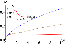
Figure 8: The DM negativity of a full phase-randomized Gaussian state is bounded by $\mathcal{B}\approx 0.0887$. The red solid line (inset as well) represents the upper bound of Eq. (S3. Testing Gaussian states under DMs) while the blue dotted and the brown dot-dashed lines represent the cases of employing $N=6$ and $N=12$ phase rotations, respectively, against $n=\sinh^{2}r$.

We plot the upper bound of Eq. (S3. Testing Gaussian states under DMs) (red solid curve) in Fig. 8, which takes maximum $\mathcal{B}_{\rm G}\approx 0.0887$. Due to the convexity of the DM negativity, we can further say that all Gaussian states and their mixtures also obey the same inequality. Therefore, if a state under a full phase-randomization violates the inequality as $\mathcal{N}_{\mathcal{D}[\rho]}>\mathcal{B}_{\rm G}$, it is a clear signature of genuine non-Gaussianity. For example, all Fock states achieve DM negativity above the Gaussian bound as shown in Fig. 9. Our method can detect genuine non-Gaussianity even for states having a non-negative Wigner function as shown in main text.

We can also numerically find the Gaussian bound for the case of finite $N$ phase-rotations, i.e. $\sigma^{\prime}\equiv\frac{1}{N}\sum_{k=0}^{N-1}e^{-i\theta_{k}{\hat{n}}}\rho_{\rm G}e^{i\theta_{k}{\hat{n}}}$ with $\theta_{k}\equiv\frac{k}{N}\pi$. In Fig. 8, the cases of $N=6$ and $N=12$ are plotted against energy $n$.

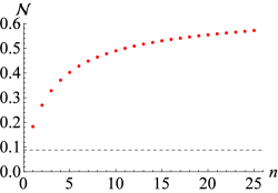
Figure 9: The DM negativity of each Fock state (red dot) is greater than the Gaussian bound $\mathcal{B}\approx 0.0887$ (black dashed).

S4. Properties of DM negativity as a measure of nonclassicality

Let us first define our DM negativity for each measured distribution as

$$\mathcal{N}_{\mathrm{DM}}^{\theta}(\rho)\equiv\frac{||\rho_{\mathrm{DM}}^{\theta}||_{1}-1}{2},$$ (29)

where $||\cdot||_{1}$ represents a trace norm and $\rho_{\mathrm{DM}}^{\theta}$ the fictitious density matrix obtained by applying our DM method to the marginal distribution measured at angle $\theta$. It satisfies the following properties:

1. $\mathcal{N}_{\mathrm{DM}}^{\theta}(\rho)=0$ for classical states.

2. $\mathcal{N}_{\mathrm{DM}}^{\theta}(\sum_{j}p_{j}\rho_{j})\leq\sum_{j}p_{j}\mathcal{N}_{\mathrm{DM}}^{\theta}(\rho_{j})$.

3. $\mathcal{N}_{\mathrm{DM}}^{\theta}(\hat{D}(\alpha)\rho\hat{D}^{{\dagger}}(\alpha))=\mathcal{N}_{\mathrm{DM}}^{\theta}(\rho)$.

[P1] In the main text, we already showed that $\rho_{\mathrm{DM}}^{\theta}$ becomes a physical state when the initial state is classical, i.e. $||\rho_{\mathrm{DM}}^{\theta}||_{1}=1$ giving $\mathcal{N}_{\mathrm{DM}}^{\theta}=0$.

[P2] We can derive the convexity of DM negativity from the fact that the trace norm satisfies the homogeneity, i.e., $||cM||_{1}=|c|||M||_{1}$, and the triangle inequality, i.e., $||M+N||_{1}\leq||M||_{1}+||N||_{1}$ Vidal2002 ; Plenio2002 .

$$\mathcal{N}_{\mathrm{DM}}^{\theta}(\sum_{j}p_{j}\rho_{j}) =\frac{||\sum_{j}p_{j}\rho_{j,\mathrm{DM}}^{\theta}||_{1}-1}{2}$$

$$\leq\frac{\sum_{j}p_{j}||\rho_{j,\mathrm{DM}}^{\theta}||_{1}-1}{2}$$

$$=\sum_{j}p_{j}\mathcal{N}_{\mathrm{DM}}^{\theta}(\rho_{j}).$$

[P3] A displacement operation only shifts the center of Wigner function and marginal distributions.

$$M_{\hat{D}(\alpha)\rho\hat{D}^{{\dagger}}(\alpha)}(q_{\theta}) =\int dp_{\theta}W_{\hat{D}(\alpha)\rho\hat{D}^{{\dagger}}(\alpha)}(q,p)$$

$$=\int dp_{\theta}W_{\rho}(q-\mathrm{Re}[\alpha],p-\mathrm{Im}[\alpha])$$

$$=M_{\rho}(q_{\theta}-\mathrm{Re}[\alpha e^{-i\theta}]).$$ (30)

DM thereby yields a displaced version $\overline{\rho}_{DM}^{\theta}=\hat{D}(\overline{\alpha})\rho_{DM}^{\theta}\hat{D}^{{\dagger}}(\overline{\alpha})$ for the displaced state $\overline{\rho}=\hat{D}(\alpha)\rho\hat{D}^{{\dagger}}(\alpha)$ with $\overline{\alpha}=\mathrm{Re}[\alpha e^{-i\theta}]$, which therefore does not affect the physicality of the output density operator. As the eigenspectrum of a Hermitian operator is invariant under a unitary operator, we conclude that $\mathcal{N}_{\mathrm{DM}}^{\theta}(\hat{D}(\alpha)\rho\hat{D}^{{\dagger}}(\alpha))=\mathcal{N}_{\mathrm{DM}}^{\theta}(\rho)$.

While a phase rotation is also a classicality preserving operation, i.e., $e^{i\hat{n}\phi}\ket{\alpha}=\ket{\alpha e^{i\phi}}$, it can increase the value of $\mathcal{N}_{\mathrm{DM}}^{\theta}[\rho]$ as the degree of DM negativity depends on the measured angle $\theta$. Thus, to make the measure invariant under phase rotations as well, we introduce an optimized version of DM negativity as

$$\mathcal{N}_{\mathrm{DM}}(\rho)=\max_{\theta\in(0,\pi)}\mathcal{N}_{\mathrm{DM}}^{\theta}(\rho).$$ (31)

The DM negativity then satisfies

1. $\mathcal{N}_{\mathrm{DM}}(\rho)=0$ for classical states.

2. $\mathcal{N}_{\mathrm{DM}}(\sum_{j}p_{j}\rho_{j})\leq\sum_{j}p_{j}\mathcal{N}_{\mathrm{DM}}(\rho_{j})$.

3. $\mathcal{N}_{\mathrm{DM}}(\hat{U}_{c}\rho\hat{U}_{c}^{{\dagger}})=\mathcal{N}_{\mathrm{DM}}(\rho)$ where $\hat{U}_{c}$ is a classicality preserving unitary operation, i.e., displacement and phase rotation.

[P1’] It is a direct consequence of [P1].

[P2’] We also obtain the convexity of optimized DM negativity from [P2].

$$\mathcal{N}_{\mathrm{DM}}(\sum_{j}p_{j}\rho_{j}) =\max_{\theta\in(0,\pi)}\mathcal{N}_{\mathrm{DM}}^{\theta}(\sum_{j}p_{j}\rho_{j})$$

$$\leq\max_{\theta\in(0,\pi)}\bigg{(}\sum_{j}p_{j}\mathcal{N}_{\mathrm{DM}}^{\theta}(\rho_{j})\bigg{)}$$

$$\leq\sum_{j}p_{j}\bigg{(}\max_{\theta\in(0,\pi)}\mathcal{N}_{\mathrm{DM}}^{\theta}(\rho_{j})\bigg{)}$$

$$=\sum_{j}p_{j}\mathcal{N}_{\mathrm{DM}}(\rho_{j}).$$

[P3’] The property [P3] implies that $\mathcal{N}_{\mathrm{DM}}(\hat{D}(\alpha)\rho\hat{D}^{{\dagger}}(\alpha))=\mathcal{N}_{\mathrm{DM}}(\rho)$. As a phase rotation only rotates the marginal distributions, i.e., $\mathcal{N}_{\mathrm{DM}}^{\theta}(e^{-i\hat{n}\phi}\rho e^{i\hat{n}\phi})=\mathcal{N}_{\mathrm{DM}}^{\theta+\phi}(\rho)$, the DM negativity optimized over the angles is not changed at all. Combining 2 and 3, we also deduce that

4. $\mathcal{N}_{\mathrm{DM}}$ does not increase under generic classicality preserving operations (mixture of unitary operations).

Let us here look into other nonclassicality measures in the literature considering the above properties. Note that nonclassical depth Lee1991 does not satisfy the convexity. As an example, a mixture of vacuum and a squeezed state, i.e., $\sigma=(1-p)|0\rangle\langle 0|+p|\psi\rangle\langle\psi|$, satisfies that $\tau(\sigma)=\tau(|\psi\rangle\langle\psi|)\neq 0$ for $0<p\leq 1$ and $\tau(\sigma)=0$ for $p=0$.

Gehrke et al. addressed a set of conditions for a proper nonclassicality measure in Gehrke2012 . They have only addressed two conditions: (1) the measure is zero only for classical state. (2) the measure is nonincreasing for any classical Kraus operator. They also proposed a degree of nonclassicality which quantifies the number of superposition between coherent states required for representing the given state. As an example, the degree of nonclassicality for a pure state in the form $\sum_{j=0}^{d}c_{j}\ket{\alpha_{j}}$ is $d$. Similar to the case of nonclassical depth, the degree of nonclassicalty does not satisfy the convexity. For example, a mixture of vacuum ($d=0$) and a pure state $\ket{\psi}$ with non-zero degree $k$, $\sigma=(1-p)|0\rangle\langle 0|+p|\psi\rangle\langle\psi|$, satisfies that $d(\sigma)=k$ for $0<p\leq 1$ and $d(\sigma)=0$ for $p=0$.

Connection to entanglement potential— With the entanglement potential defined in the main text as

$$\mathcal{P}_{\mathrm{ent}}[\rho]\equiv\frac{||[\hat{U}_{\mathrm{BS}}(\rho_{1}\otimes|0\rangle\langle 0|_{2})\hat{U}_{\mathrm{BS}}^{{\dagger}}]^{\mathrm{PT}}||_{1}-1}{2},$$ (32)

we here prove the relation

$$\mathcal{N}_{\mathrm{DM2}}[\rho]\leq\mathcal{P}_{\mathrm{ent}}[\rho].$$ (33)

To this aim, we slightly modify the procedures in the main text as follows. After the beam-splitting operation for entanglement generation, we perform local unitary operations $e^{-i\theta\hat{n}_{1}}\otimes e^{-i\theta\hat{n}_{2}}$, which has no effect on entanglement and simply rotates the output Wigner function in Eq. (7) of main text as

$$W_{\rho}(q_{+}\cos\theta-p_{+}\sin\theta,q_{+}\sin\theta+p_{+}\cos\theta)$$

$$\times W_{|0\rangle\langle 0|}(q_{-}\cos\theta-p_{-}\sin\theta,q_{-}\sin\theta+p_{-}\cos\theta)$$

$$= W_{\rho}(q_{+}\cos\theta-p_{+}\sin\theta,q_{+}\sin\theta+p_{+}\cos\theta)$$

$$\times W_{|0\rangle\langle 0|}(q_{-},p_{-}),$$ (34)

where $q_{\pm}=\frac{1}{\sqrt{2}}(q_{1}\pm q_{2})$, $p_{\pm}=\frac{1}{\sqrt{2}}(p_{1}\pm p_{2})$, together with the fact that the Wigner function for vacuum is invariant under rotation. PT and BS operations change it to

$$\xrightarrow{\mathrm{PT}} W_{\rho}(q_{+}\cos\theta-p_{-}\sin\theta,q_{+}\sin\theta+p_{-}\cos\theta)$$

$$\times W_{|0\rangle\langle 0|}(q_{-},p_{+})$$

$$\xrightarrow{\mathrm{BS}} W_{\rho}(q_{1}\cos\theta-p_{2}\sin\theta,q_{1}\sin\theta+p_{2}\cos\theta)$$

$$\times W_{|0\rangle\langle 0|}(q_{2},p_{1}).$$ (35)

Integrating over $q_{2}$ and $p_{2}$, we obtain the marginal Wigner function for one mode as $M_{\rho}(x_{1})M_{|0\rangle\langle 0|}(y_{1})$, which represents the demarginalization of the single mode state $\rho$ in Eq. (2) along with the rotated axis $x_{1}=q_{1}\cos\theta+p_{1}\sin\theta$.

As a unitary operation preserves the eigenspectrum of an input state, we have

$$||\rho^{\prime}||_{1}=||\hat{U}_{\mathrm{BS}}\rho^{\prime}\hat{U}_{\mathrm{BS}}^{{\dagger}}||_{1},$$ (36)

where $\rho^{\prime}=[\hat{R}(\theta)\hat{U}_{\mathrm{BS}}(\rho_{1}\otimes|0\rangle\langle 0|_{2})\hat{U}_{\mathrm{BS}}^{{\dagger}}\hat{R}^{{\dagger}}(\theta)]^{\mathrm{PT}}$ and $\hat{R}(\theta)=e^{-i\theta\hat{n}_{1}}\otimes e^{-i\theta\hat{n}_{2}}$. Using the fact that trace norm is nonincreasing under partial trace Vidal2002 ; Plenio2002 , e.g., $||\rho_{AB}||_{1}\geq||\rho_{A}||_{1}$, we obtain

$$||\rho^{\prime}||_{1}\geq||\mathrm{Tr}_{2}[\hat{U}_{\mathrm{BS}}\rho^{\prime}\hat{U}_{\mathrm{BS}}^{{\dagger}}]||_{1},$$ (37)

which is satisfied for every rotation angle $\theta$. From the obtained inequality, we derive the relation in Eq. (33).

Furthermore, we can also show that two measures are identical for a Gaussian state, $\mathcal{N}_{\mathrm{DM2}}[\sigma]=\mathcal{P}_{\mathrm{ent}}[\sigma]$ by direct calculations.

S5. All FDS can be detected via a single marginal distribution regardless of measurement axis.

• Derivation of Wigner function for FDS

The Wigner function of the FDS $\rho=\sum_{j,k=0}^{N}\rho_{jk}|j\rangle\langle k|$ is given by

$$W_{\rho}(x,y)=\sum_{j,k=0}^{N}\rho_{jk}W_{|j\rangle\langle k|}(x,y),$$ (38)

where $W_{|j\rangle\langle k|}(x,y)$ represents the operator $|j\rangle\langle k|$

$$W_{|j\rangle\langle k|}(x,y)=\frac{2}{\pi}e^{-2|\alpha_{\theta}|^{2}}\sqrt{\frac{k!}{j!}}(-1)^{k}(2\alpha_{\theta}^{*})^{j-k}L_{k}^{(j-k)}(4|\alpha_{\theta}|^{2})\hskip 2.84544pt(j\geq k),$$ (39)

with $L_{n}^{(\alpha)}(z)$ a generalized Laguerre polynomial of order $n$, $\alpha_{\theta}=(x+iy)e^{-i\theta}$ and $W_{|j\rangle\langle k|}(x,y)=W_{|k\rangle\langle j|}^{*}(x,y)$ for $j<k$, as shown in Ref. UL . With $\alpha_{\theta=0}=q+ip$, we have a simple relation $W_{|j\rangle\langle k|}(x,y)=e^{i\theta(j-k)}W_{|j\rangle\langle k|}(q,p)$, thus we are only concerned with $W_{|j\rangle\langle k|}(q,p)$ letting $\theta=0$.

We first reexpress Eq. (39) using $\frac{d^{k}}{dx^{k}}L_{n}^{(\alpha)}(x)=(-1)^{k}L_{n-k}^{(\alpha+k)}(x)$,

$$W_{|j\rangle\langle k|}(q,p) =\frac{2}{\pi}e^{-2q^{2}-2p^{2}}\sqrt{\frac{k!}{j!}}(-1)^{k}(2q-2ip)^{j-k}L_{k}^{(j-k)}(4q^{2}+4p^{2})$$

$$=\frac{2}{\pi}e^{-2q^{2}-2p^{2}}\sqrt{\frac{k!}{j!}}\frac{(-1)^{j}}{2^{j-k}}\bigg{[}\frac{\partial^{j-k}}{\partial\alpha^{j-k}}L_{j}(4\alpha\alpha^{*})\bigg{]}_{\alpha=q+ip}.$$ (40)

Employing the formulas in Ref. AS , i.e. $L_{n}^{(\alpha+\beta+1)}(x+y)=\sum_{j=0}^{n}L_{j}^{(\alpha)}(x)L_{n-j}^{(\beta)}(y)$ and $H_{2n}(x)=(-4)^{n}n!L_{n}^{(-1/2)}(x^{2})$, we obtain

$$L_{j}(4q^{2}+4p^{2}) =\sum_{\ell=0}^{j}L_{\ell}^{(-1/2)}(4q^{2})L_{j-\ell}^{(-1/2)}(4p^{2})$$

$$=\sum_{\ell=0}^{j}\frac{H_{2\ell}(2q)H_{2(j-\ell)}(2p)}{(-4)^{j}\ell!(j-\ell)!}.$$ (41)

Combining Eqs. (S5. All FDS can be detected via a single marginal distribution regardless of measurement axis.) and (S5. All FDS can be detected via a single marginal distribution regardless of measurement axis.) with $\frac{d}{dx}H_{n}(x)=2nH_{n-1}(x)$ and $\frac{d^{n+1}}{dx^{n+1}}H_{n}(x)=0$, we obtain

$$W_{|j\rangle\langle k|}(q,p) =\frac{2}{\pi}e^{-2q^{2}-2p^{2}}\sqrt{\frac{k!}{j!}}\frac{(-1)^{j}}{2^{j-k}}\bigg{[}\frac{\partial^{j-k}}{\partial\alpha^{j-k}}\sum_{\ell=0}^{j}\frac{H_{2\ell}(\alpha^{*}+\alpha)H_{2(j-\ell)}(i\alpha^{*}-i\alpha)}{(-4)^{j}\ell!(j-\ell)!}\bigg{]}_{\alpha=q+ip}$$

$$=\frac{2}{\pi}e^{-2q^{2}-2p^{2}}\sqrt{\frac{k!}{j!}}\frac{(-1)^{j}}{2^{j-k}}\sum_{\ell=0}^{j}\bigg{[}\sum_{m=s}^{t}\frac{1}{(-4)^{j}\ell!(j-\ell)!}\frac{(j-k)!}{m!(j-k-m)!}\frac{2^{m}(2\ell)!}{(2\ell-m)!}H_{2\ell-m}(\alpha^{*}+\alpha)$$

$$\times\frac{(-2i)^{j-k-m}\{2(j-\ell)\}!}{\{2(j-\ell)-(j-k-m)\}!}H_{2(j-\ell)-(j-k-m)}(i\alpha^{*}-i\alpha)\bigg{]}_{\alpha=q+ip}$$

$$=\frac{2}{\pi}e^{-2q^{2}-2p^{2}}\sqrt{\frac{k!}{j!}}\frac{1}{4^{j}}\frac{(j-k)!}{j!}\sum_{\ell=0}^{j}\sum_{m=s}^{t}\binom{j}{\ell}\binom{2\ell}{m}\binom{2(j-\ell)}{j-k-m}\frac{H_{2\ell-m}(2q)H_{j+k+m-2\ell}(2p)}{i^{j-k-m}},$$ (42)

with $s=\max[0,2\ell-j-k]$ and $t=\min[j-k,2\ell]$, where we used $\frac{d^{n}}{dx^{n}}[f(x)g(x)]=\sum_{s=0}^{n}\frac{n!}{(n-s)!s!}\frac{d^{n-s}f}{dx^{n-s}}\frac{d^{s}g}{dx^{s}}$. Finally, we can recast Eq. (S5. All FDS can be detected via a single marginal distribution regardless of measurement axis.) to

$$W_{|j\rangle\langle k|}(q,p)=\frac{2}{\pi}e^{-2q^{2}-2p^{2}}\sum_{n=0}^{j+k}A_{|j\rangle\langle k|}(n)H_{n}(2q)H_{j+k-n}(2p),$$ (43)

where

$$A_{|j\rangle\langle k|}(n) =\sqrt{\frac{k!}{j!}}\frac{1}{4^{j}}\frac{(j-k)!}{j!}\sum_{\ell=0}^{j}\sum_{m=s}^{t}\binom{j}{\ell}\binom{2\ell}{m}\binom{2(j-\ell)}{j-k-m}\frac{\delta_{n,2\ell-m}}{i^{j-k-m}}$$

$$=\begin{cases}\displaystyle\sqrt{\frac{k!}{j!}}\frac{1}{4^{j}}\frac{(j-k)!}{j!}\sum_{\ell=\lceil\frac{n}{2}\rceil}^{\lfloor\frac{j-k+n}{2}\rfloor}\binom{j}{\ell}\binom{2\ell}{2\ell-n}\binom{2(j-\ell)}{j-k+n-2\ell}\frac{(-1)^{\ell}}{i^{j-k+n}}&\mbox{for $j>k$,}\\ \displaystyle\frac{1}{4^{j}(\frac{n}{2})!(j-\frac{n}{2})!}&\mbox{for $j=k$ and even $n$,}\\ \displaystyle 0&\mbox{for $j=k$ and odd $n$.}\end{cases}$$ (44)

We also provide an alternative expression of $A_{|j\rangle\langle k|}(n)$ for even $j+k-n$ as

$$A_{|j\rangle\langle k|}(n)=\frac{(-1)^{\frac{j+k-n}{2}}\sqrt{j!k!}}{2^{j+k}n!(j+k-n)!}\sum_{r=0}^{n}(-1)^{k-r}\binom{n}{r}\binom{j+k-n}{k-r}.$$ (45)

This can be obtained by comparing two methods of deriving marginal distribution for $|j\rangle\langle k|$, that is, $M_{|j\rangle\langle k|}(q)=\int dpW_{|j\rangle\langle k|}(q,p)$ and $M_{|j\rangle\langle k|}(q)=\braket{q}{j}\braket{k}{q}$, where $\ket{q}$ is an eigenstate of the position operator, $\hat{q}\ket{q}=q\ket{q}$. Using the formula in Ref. Wang2008 , $H_{j}(x)H_{k}(x)=\sum_{n=0}^{j+k}a_{jk}(n)H_{n}(\sqrt{2}x)$ with

$$a_{jk}(n)=\begin{cases}\frac{(-1)^{\frac{j+k-n}{2}}j!k!}{2^{\frac{j+k}{2}}n!(\frac{j+k-n}{2})!}\sum_{r=0}^{n}(-1)^{k-r}\binom{n}{r}\binom{j+k-n}{k-r}&\mbox{for even $j+k-n$,}\\ 0&\mbox{for odd $j+k-n$,}\end{cases}$$ (46)

and the expression in Ref. BR , $\braket{q}{n}=(\frac{2}{\pi})^{\frac{1}{4}}\sqrt{\frac{1}{2^{n}n!}}e^{-q^{2}}H_{n}(\sqrt{2}q)$, we obtain

$$\braket{q}{j}\braket{k}{q} =\sqrt{\frac{2}{\pi}}\frac{1}{2^{\frac{j+k}{2}}\sqrt{j!k!}}e^{-2q^{2}}H_{j}(\sqrt{2}q)H_{k}(\sqrt{2}q),$$

$$=\sqrt{\frac{2}{\pi}}e^{-2q^{2}}\sum_{n=0}^{j+k}\frac{a_{jk}(n)}{2^{\frac{j+k}{2}}\sqrt{j!k!}}H_{n}(2q).$$ (47)

On the other hand, from Eq. (43), we obtain

$$\int_{-\infty}^{\infty}dpW_{|j\rangle\langle k|}(q,p) =\begin{cases}\sqrt{\frac{2}{\pi}}e^{-2q^{2}}\sum_{m=0}^{\frac{j+k}{2}}\frac{(j+k-2m)!}{(\frac{j+k}{2}-m)!}A_{|j\rangle\langle k|}(2m)H_{2m}(2q)&\mbox{for even $j+k$,}\\ \sqrt{\frac{2}{\pi}}e^{-2q^{2}}\sum_{m=0}^{\frac{j+k-1}{2}}\frac{(j+k-2m-1)!}{(\frac{j+k-1}{2}-m)!}A_{|j\rangle\langle k|}(2m+1)H_{2m+1}(2q)&\mbox{for odd $j+k$,}\end{cases}$$

$$=\sqrt{\frac{2}{\pi}}e^{-2q^{2}}\sum_{m^{\prime}=0}^{\left[\frac{j+k}{2}\right]}\frac{(2m^{\prime})!}{m^{\prime}!}A_{|j\rangle\langle k|}(j+k-2m^{\prime})H_{j+k-2m^{\prime}}(2q),$$ (48)

where we have used $\int_{-\infty}^{\infty}dxe^{-2x^{2}}H_{2m}(2x)=\sqrt{\frac{\pi}{2}}\frac{(2m)!}{m!}$ and $\int_{-\infty}^{\infty}dxe^{-2x^{2}}H_{2m+1}(2x)=0$ for an integer $m\geq 0$. Comparing Eqs. (S5. All FDS can be detected via a single marginal distribution regardless of measurement axis.) and (S5. All FDS can be detected via a single marginal distribution regardless of measurement axis.), we obtain Eq. (45).

• Unphysicality of all FDSs under DM1 and DM2 methods

Starting with a FDS state $\rho=\sum_{j,k=0}^{N}\rho_{jk}|j\rangle\langle k|$ with its highest excitation $N$, i.e. $\rho_{NN}\neq 0$, the density matrix elements for $W_{\rho}^{\mathrm{DM1}}(x,y)$ under DM1 are obtained by

$$\rho_{n_{1},n_{2}}^{\prime} =\pi\int_{-\infty}^{\infty}dx\int_{-\infty}^{\infty}dyW_{\rho}^{\mathrm{DM1}}(x,y)W_{|n_{2}\rangle\langle n_{1}|}(x,y)$$

$$=\pi\int_{-\infty}^{\infty}dx\int_{-\infty}^{\infty}dy\bigg{(}\frac{2}{\pi}\bigg{)}^{2}e^{-4x^{2}-4y^{2}}\sum_{j,k=0}^{N}\rho_{jk}e^{i(j-k)\theta}\sum_{j^{\prime},k^{\prime}=0}^{N}\rho_{j^{\prime}k^{\prime}}e^{i(j^{\prime}-k^{\prime})\theta}$$

$$\times\sum_{m=0}^{\left[\frac{j+k}{2}\right]}\frac{(2m)!}{m!}A_{|j\rangle\langle k|}(j+k-2m)H_{j+k-2m}(2x)\sum_{m^{\prime}=0}^{\left[\frac{j^{\prime}+k^{\prime}}{2}\right]}\frac{(2m^{\prime})!}{m^{\prime}!}A_{|j^{\prime}\rangle\langle k^{\prime}|}(j^{\prime}+k^{\prime}-2m^{\prime})H_{j^{\prime}+k^{\prime}-2m^{\prime}}(2y)$$

$$\times\sum_{n=0}^{n_{1}+n_{2}}A_{|n_{2}\rangle\langle n_{1}|}(n)H_{n}(2x)H_{n_{1}+n_{2}-n}(2y).$$ (49)

Using the orthogonality of Hermite polynomials, $\int dxe^{-4x^{2}}H_{a}(2x)H_{b}(2x)=\sqrt{\pi}2^{b-1}b!\delta_{a,b}$, we have

$$\rho_{n_{1},n_{2}}^{\prime} =\sum_{j,k=0}^{N}\rho_{jk}e^{i(j-k)\theta}\sum_{j^{\prime},k^{\prime}=0}^{N}\rho_{j^{\prime}k^{\prime}}e^{i(j^{\prime}-k^{\prime})\theta}\sum_{m=0}^{\left[\frac{j+k}{2}\right]}\sum_{m^{\prime}=0}^{\left[\frac{j^{\prime}+k^{\prime}}{2}\right]}\sum_{n=0}^{n_{1}+n_{2}}\delta_{n,j+k-2m}\delta_{n_{1}+n_{2}-n,j^{\prime}+k^{\prime}-2m^{\prime}}$$

$$\times 2^{n_{1}+n_{2}}n!(n_{1}+n_{2}-n)!\frac{(2m)!}{m!}\frac{(2m^{\prime})!}{m^{\prime}!}A_{|j\rangle\langle k|}(n)A_{|j^{\prime}\rangle\langle k^{\prime}|}(n_{1}+n_{2}-n)A_{|n_{2}\rangle\langle n_{1}|}(n).$$ (50)

Looking into Kronecker delta functions and $j+k+j^{\prime}+k^{\prime}\leq 4N$, we first have $\rho_{n_{1},n_{2}}^{\prime}=0$ for $n_{1}+n_{2}>4N$ that naturally imposes $\rho^{\prime}_{n,n}=0$ for $n>2N$. We now derive compact expressions for $\rho_{4N,0}^{\prime}$ and $\rho_{0,4N}^{\prime}$, which correspond to $j=k=j^{\prime}=k^{\prime}=N$ and $m=m^{\prime}=0$, as

$$\rho_{4N,0}^{\prime}=\rho_{0,4N}^{\prime}=\rho_{NN}^{2}16^{N}\{(2N)!\}^{2}A_{|N\rangle\langle N|}(2N)^{2}A_{|4N\rangle\langle 0|}(2N)=\frac{\sqrt{(4N)!}}{(-16)^{N}(N!)^{2}}\rho_{NN}^{2},$$ (51)

where we have used $A_{|N\rangle\langle N|}(2N)=\frac{1}{4^{N}N!}$ and $A_{|4N\rangle\langle 0|}(2N)=\frac{\sqrt{(4N)!}}{(-16)^{n}\{(2N)!\}^{2}}$ from Eqs. (S5. All FDS can be detected via a single marginal distribution regardless of measurement axis.) and (45). For the determinant of a sub-matrix, we find that

$$\rho_{0,0}^{\prime}\rho_{4N,4N}^{\prime}-\rho_{4N,0}^{\prime}\rho_{0,4N}^{\prime}=-\frac{(4N)!}{256^{N}(N!)^{4}}\rho_{NN}^{4}<0,$$ (52)

which confirms the nonclassicality of the original FDS state $\rho=\sum_{j,k=0}^{N}\rho_{jk}|j\rangle\langle k|$.

Similarly, the density matrix elements for $W_{\rho}^{\mathrm{DM2}}(x,y)$ under DM2 are given by

$$\rho_{n_{1},n_{2}}^{\prime\prime} =\pi\int_{-\infty}^{\infty}dx\int_{-\infty}^{\infty}dyW_{\rho}^{\mathrm{DM2}}(x,y)W_{|n_{2}\rangle\langle n_{1}|}(x,y)$$

$$=\pi\int_{-\infty}^{\infty}dx\int_{-\infty}^{\infty}dy\bigg{(}\frac{2}{\pi}\bigg{)}^{2}e^{-4x^{2}-4y^{2}}\sum_{j,k=0}^{N}\rho_{jk}e^{i(j-k)\theta}$$

$$\times\sum_{m=0}^{[\frac{j+k}{2}]}\frac{(2m)!}{m!}A_{|j\rangle\langle k|}(j+k-2m)H_{j+k-2m}(2x)\sum_{n=0}^{n_{1}+n_{2}}A_{|n_{2}\rangle\langle n_{1}|}(n)H_{n}(2x)H_{n_{1}+n_{2}-n}(2y)$$

$$=\sum_{j,k=0}^{N}\rho_{jk}e^{i(j-k)\theta}\sum_{m=0}^{[\frac{j+k}{2}]}\sum_{n=0}^{n_{1}+n_{2}}\delta_{n,j+k-2m}\delta_{n_{1}+n_{2}-n,0}2^{n_{1}+n_{2}}n!\frac{(2m)!}{m!}A_{|j\rangle\langle k|}(n)A_{|n_{2}\rangle\langle n_{1}|}(n)$$

$$=\sum_{j,k=0}^{N}\rho_{jk}e^{i(j-k)\theta}\sum_{m=0}^{[\frac{j+k}{2}]}\delta_{n_{1}+n_{2},j+k-2m}2^{n_{1}+n_{2}}(n_{1}+n_{2})!\frac{(2m)!}{m!}A_{|j\rangle\langle k|}(n_{1}+n_{2})A_{|n_{2}\rangle\langle n_{1}|}(n_{1}+n_{2}),$$ (53)

which manifests that $\rho_{n_{1},n_{2}}^{\prime\prime}=0$ for $n_{1}+n_{2}>2N$. In addition, we obtain compact expressions for $\rho_{2N,0}^{\prime\prime}$ and $\rho_{0,2N}^{\prime\prime}$, for which $j=k=N$ and $m=0$, as

$$\rho_{2N,0}^{\prime\prime}=\rho_{0,2N}^{\prime\prime}=\rho_{NN}2^{2N}(2N)!A_{|N\rangle\langle N|}(2N)A_{|2N\rangle\langle 0|}(2N)=\frac{\sqrt{(2N)!}}{4^{N}N!}\rho_{NN},$$ (54)

where $A_{|2N\rangle\langle 0|}(2N)=\frac{1}{4^{N}\sqrt{(2N)!}}$ from Eq. (45). This leads to

$$\rho_{0,0}^{\prime\prime}\rho_{2N,2N}^{\prime\prime}-\rho_{2N,0}^{\prime\prime}\rho_{0,2N}^{\prime\prime}=0-\frac{(2N)!}{16^{N}(N!)^{2}}\rho_{N,N}^{2}<0,$$ (55)

again confirming the nonclassicality of the original state. Note that the above results under both of DM1 and DM2 hold regardless of $\theta$ (quadrature axis), which makes our criteria experimentally favorable. That is, the nonclassicality for an arbitrary FDS state can be verified by observing a single marginal distribution along any directions.

S6. Detection of non-Gaussian states in infinite dimension

We here consider the detection of nonclassicality for non-Gaussian states in infinite dimension, which has practical relevance to CV quantum information processing. In particular, we examine those non-Gaussian states without squeezing effect in order to demonstrate the merit of our formalism while employing a marginal distribution.

(i) photon-added coherent state $\hat{a}^{{\dagger}}\ket{\gamma}$— We note that a photon-added coherent state do not have squeezing effect for $|\gamma|<1$ Agarwal1991 , which restricts the detection of its nonclassicality under a variance test. In contrast, our criteria detect it for all $\gamma$. We can recast the state as a displaced FDS,

$$\hat{a}^{{\dagger}}\hat{D}(\gamma)\ket{0} =\hat{D}(\gamma)(\hat{a}^{{\dagger}}+\gamma^{*})\ket{0}$$

$$=\hat{D}(\gamma)(\ket{1}+\gamma^{*}\ket{0}),$$ (56)

where we have used $\hat{D}(\gamma)\hat{a}^{{\dagger}}\hat{D}^{{\dagger}}(\gamma)=\hat{a}^{{\dagger}}+\gamma^{*}$. As our DM criteria are able to detect every FDS and invariant under displacement operation, we can detect every photon added coherent state using our criteria. Remarkably, our DM methods successfully detect its nonclassicality regardless of quadrature axis as for the case of FDS.

(ii) photon-added thermal state $\rho=\hat{a}^{{\dagger}}\rho_{\mathrm{th}}(\bar{n})\hat{a}$— Its Wigner function is given by

$$W_{\rho}(q,p) =\frac{2}{\pi}\exp\bigg{[}-\frac{2(q^{2}+p^{2})}{1+2n}\bigg{]}$$

$$\times\frac{4(1+n)(q^{2}+p^{2})-(1+2n)}{(1+2n)^{3}},$$ (57)

with its marginal distribution given by

$$M_{\rho}(x) =\sqrt{\frac{2}{\pi}}\exp\bigg{(}-\frac{2q^{2}}{1+2n}\bigg{)}$$

$$\times\frac{n(1+2n)+4(1+n)q^{2}}{(1+2n)^{5/2}}.$$ (58)

Applying DM method to the marginal distribution and obtaining relevant density matrix elements, we consider $\{\ket{0},\ket{4}\}$ subspace for DM1,

$$\begin{pmatrix}\dfrac{1}{4(1+n)}&-\dfrac{\sqrt{\frac{3}{2}}}{4(1+n)^{3}}\\ -\dfrac{\sqrt{\frac{3}{2}}}{4(1+n)^{3}}&\dfrac{n^{2}(6+8n+n^{2})}{4(1+n)^{5}}\end{pmatrix},$$ (59)

and $\{\ket{0},\ket{2}\}$ subspace for DM2,

$$\begin{pmatrix}\dfrac{1}{2\sqrt{1+n}}&\dfrac{2+n}{4\sqrt{2}(1+n)^{3/2}}\\ \dfrac{2+n}{4\sqrt{2}(1+n)^{3/2}}&\dfrac{3n(4+n)}{16(1+n)^{5/2}}\end{pmatrix},$$ (60)

then a negative eigenvalue can be found at low mean photon number $n\lesssim 0.40$ and $n\lesssim 0.45$, respectively. For a higher mean photon number, we need to investigate density matrix elements with higher Fock numbers.

(iii) Dephased odd cat states—$\rho_{\mathrm{odd}}\sim|\gamma\rangle\langle\gamma|+|-\gamma\rangle\langle-\gamma|-f(|\gamma\rangle\langle-\gamma|+|-\gamma\rangle\langle\gamma|)$ where $\ket{\gamma}$ is a coherent state with amplitude $\gamma$ and $1-f$ denotes the degree of dephasing. They show no squeezing for all $\gamma>0$ and $f>0$. As we obtain the density matrix elements for $\mathcal{D}_{j}[W_{\rho_{\mathrm{odd}}}](x,y)$ employing the marginal distribution for the rotated quadrature $q_{\theta}$,

$$M_{\rho_{\mathrm{odd}}}(q_{\theta})= \sqrt{\frac{2}{\pi}}e^{-2q_{\theta}^{2}-2\gamma^{2}\cos^{2}\theta}$$

$$\times \frac{\cosh(4\gamma q_{\theta}\cos\theta)-f\cos(4\gamma q_{\theta}\sin\theta)}{1-fe^{-2\gamma^{2}}},$$ (61)

we find a non-positive submatrix for $\gamma>0$ and $f>0$. More explicitly, for the case of $\mathcal{D}_{1}[W_{\rho_{\mathrm{odd}}}]=W_{\rho_{\mathrm{odd}}^{\prime}}$, we find negativity in $\{\ket{0},\ket{4}\}$ subspace,

$$\bra{0}\rho_{\mathrm{odd}}^{\prime}\ket{0} =\frac{e^{2\gamma^{2}\sin^{2}\theta}(e^{\gamma^{2}}-f)^{2}}{(e^{2\gamma^{2}}-f)^{2}},$$

$$\bra{0}\rho_{\mathrm{odd}}^{\prime}\ket{4} =\bra{4}\rho_{\mathrm{odd}}^{\prime\prime}\ket{0}$$

$$=-\frac{\gamma^{4}e^{2\gamma^{2}\sin^{2}\theta}}{4\sqrt{6}(e^{2\gamma^{2}}-f)^{2}}\{3(e^{\gamma^{2}}+f)^{2}$$

$$+4(e^{2\gamma^{2}}-f)\cos(2\theta)+(e^{\gamma^{2}}-f)^{2}\cos(4\theta)\},$$

$$\bra{4}\rho_{\mathrm{odd}}^{\prime}\ket{4} =\frac{\gamma^{8}e^{2\gamma^{2}\sin^{2}\theta}}{12(e^{2\gamma^{2}}-f)^{2}}[8e^{2\gamma^{2}}\cos^{8}\theta$$

$$+f\{-e^{\gamma^{2}}\cos^{4}(2\theta)+8f\sin^{8}\theta\}],$$ (62)

particularly its negative determinant

$$\bra{0}\rho_{\mathrm{odd}}^{\prime}\ket{0}\bra{4}\rho_{\mathrm{odd}}^{\prime}\ket{4}-|\bra{0}\rho_{\mathrm{odd}}^{\prime\prime}\ket{4}|^{2}$$

$$=-\frac{fe^{\gamma^{2}(1+4\sin^{2}\theta)}\gamma^{8}}{12(e^{2\gamma^{2}}-f)^{4}}\{9(e^{2\gamma^{2}}+f^{2})$$

$$+12(e^{2\gamma^{2}}-f^{2})\cos(2\theta)+4(e^{\gamma^{2}}-f)^{2}\cos(4\theta)\},$$ (63)

for all $\gamma>0$ and $f>0$ independent of the quadrature axis. Note that $9(e^{2\gamma^{2}}+f^{2})+12(e^{2\gamma^{2}}-f^{2})t^{2}+4(e^{\gamma^{2}}-f)^{2}(2t^{2}-1)$ is positive for every $t$.

For the case of $\mathcal{D}_{2}[W_{\rho_{\mathrm{odd}}}]=W_{\rho_{\mathrm{odd}}^{\prime\prime}}$, we obtain density matrix elements in $\{\ket{0},\ket{2}\}$ subspace as

$$\bra{0}\rho_{\mathrm{odd}}^{\prime\prime}\ket{0} =\frac{e^{\gamma^{2}\sin^{2}\theta}(e^{\gamma^{2}}-f)}{e^{2\gamma^{2}}-f},$$

$$\bra{0}\rho_{\mathrm{odd}}^{\prime\prime}\ket{2} =\bra{2}\rho_{\mathrm{odd}}^{\prime\prime}\ket{0}$$

$$=\frac{\gamma^{2}e^{\gamma^{2}\sin^{2}\theta}(e^{\gamma^{2}}\cos^{2}\theta+f\sin^{2}\theta)}{\sqrt{2}(e^{2\gamma^{2}}-f)},$$

$$\bra{2}\rho_{\mathrm{odd}}^{\prime\prime}\ket{2} =\frac{e^{\gamma^{2}\sin^{2}\theta}\gamma^{4}(e^{\gamma^{2}}\cos^{4}\theta-f\sin^{4}\theta)}{2(e^{2\gamma^{2}}-f)},$$ (64)

with its negative determinant

$$\bra{0}\rho_{\mathrm{odd}}^{\prime\prime}\ket{0}\bra{2}\rho_{\mathrm{odd}}^{\prime\prime}\ket{2}-|\bra{0}\rho_{\mathrm{odd}}^{\prime\prime}\ket{2}|^{2}$$

$$=-\frac{fe^{\gamma^{2}(1+2\sin^{2}\theta)}\gamma^{4}}{2(e^{2\gamma^{2}}-f)^{2}},$$ (65)

for all $\gamma>0$ and $f>0$ independent of the quadrature axis.

References

- (1) Braunstein SL, Van Loock P (2005) Quantum information with continuous variables, Rev Mod Phys 77:513.
- (2) Cerf N, Leuchs G, Polzik ES (2007) Quantum Information with Continuous Variables of Atoms and Light (Imperial College Press, London).
- (3) Weedbrook C, Pirandola S, García-Patrón R, Cerf NJ, Ralph TC, Shapiro JH, Lloyd S (2012) Gaussian quantum information, Rev Mod Phys 84:621.
- (4) Richter Th, Vogel W (2002) Nonclassicality of Quantum States: A Hierarchy of Observable Conditions, Phys Rev Lett 89:283601.
- (5) Ryl S, Sperling J, Agudelo E, Mraz M, Köhnke S, Hage B, Vogel W (2015) Unified nonclassicality criteria, Phys Rev A 92:011801.
- (6) Mari A, Kieling K, Nielsen BM, Polzik ES, Eisert J (2011) Directly Estimating Nonclassicality, Phys Rev Lett 106:010403.
- (7) Park J, Zhang J, Lee J, Ji SW, Um M, Lv D, Kim K, Nha H (2015) Testing Nonclassicality and Non-Gaussianity in Phase Space, Phys Rev Lett 114:190402.
- (8) Park J, Nha H (2015) Demonstrating nonclassicality and non-Gaussianity of single-mode fields: Bell-type tests using generalized phase-space distributions, Phys Rev A 92:062134.
- (9) Glauber RJ (1963) Coherent and Incoherent States of the Radiation Field, Phys. Rev. 131:2766.
- (10) Sudarshan ECG (1963) Equivalence of Semiclassical and Quantum Mechanical Descriptions of Statistical Light Beams, Phys. Rev. Lett. 10:277.
- (11) Lvovsky AI, Raymer MG (2009) Continuous-variable optical quantum-state tomography, Rev Mod Phys 81:299.
- (12) D’Ariano GM, Macchiavello C, Paris MGA (1994) Detection of the density matrix through optical homodyne tomography without filtered back projection, Phys Rev A 50:4298.
- (13) Hradil Z (1997) Quantum-state estimation, Phys Rev A 55:R1561.
- (14) Banaszek K, D’Ariano GM, Paris MGA, Sacchi MF (1999) Maximum-likelihood estimation of the density matrix, Phys Rev A 61:010304.
- (15) Řeháček J, Mogilevtsev D, Hradil Z (2010) Operational Tomography: Fitting of Data Patterns, Phys Rev Lett 105:010402.
- (16) Teo YS, Zhu H, Englert BG, Řeháček J, Hradil Z (2011) Quantum-State Reconstruction by Maximizing Likelihood and Entropy, Phys Rev Lett 107:020404.
- (17) Shchukin E, Richter Th, Vogel W (2005) Nonclassicality criteria in terms of moments, Phys Rev A 71:011802.
- (18) Shchukin EV, Vogel W (2005) Nonclassical moments and their measurement, Phys Rev A 72:043808.
- (19) Bednorz A, Belzig W (2011) Forth moments reveal the negativity of the Wigner function, Phys Rev A 83:052113.
- (20) For Gaussian states, our method, if directly applied, works only for the squeezed axes not covering the whole range of quadrature axis. As we show in supple , however, a phase-randomization, which does not create nonclassicality, modifies a Gaussian state to a non-Gaussian state for which nonclassicality can be detected regardless of quadrature axis.
- (21) Asbóth JK, Calsamiglia J, Ritsch H (2005) Computable Measure of Nonclassicality for Light, Phys Rev Lett 94:173602.
- (22) Kim MS, Son W, Bužek V, Knight PL (2002) Entanglement by a beam splitter: Nonclassicality as a prerequisite for entanglement, Phys Rev A 65:032323.
- (23) Xiang-bin W (2002) Theorem for the beam-splitter entangler, Phys Rev A 66:024303.
- (24) Tahira R, Ikram M, Nha H, Zubairy MS (2009) Entanglement of Gaussian states using a beam splitter, Phys Rev A 79:023816.
- (25) Peres A (1996) Separability Criterion for Density Matrices, Phys Rev Lett 77:1413.
- (26) Horodecki M, Horodecki P, Horodecki R (1996) Separability of mixed states: necessary and sufficient conditions, Phys Lett A 223:1.
- (27) Duan LM, Giedke G, Cirac JI, Zoller P (2000) Inseparability Criterion for Continuous Variable Systems, Phys Rev Lett 84:2722.
- (28) Simon R (2000) Peres-Horodecki Separability Criterion for Continuous Variable Systems, Phys Rev Lett 84:2726.
- (29) Shchukin E, Vogel W (2005) Inseparability Criteria for Continuous Bipartite Quantum States, Phys Rev Lett 95:230502.
- (30) Miranowicz A, Piani M, Horodecki P, Horodecki R (2009) Inseparability criteria based on matrices of moments, Phys Rev A 80:052303.
- (31) Walborn SP, Taketani BG, Salles A, Toscano F, Filho RLM (2009) Entropic Entanglement Criteria for Continuous Variables, Phys Rev Lett 103:160505.
- (32) Saboia A, Toscano F, Walborn SP (2011) Family of continuous-variable entanglement criteria using general entropy functions Phys Rev A 83:032307.
- (33) Nha H, Zubairy MS (2008) Uncertainty Inequalities as Entanglement Criteria for Negative Partial-Transpose States, Phys Rev Lett 101:130402.
- (34) Nha H, Lee SY, Ji SW, Kim MS (2012) Efficient Entanglement Criteria beyond Gaussian Limits Using Gaussian Measurements, Phys Rev Lett 108:030503.
- (35) Horodecki M, Horodecki P, Horodecki R (1998) Mixed-State Entanglement and Distillation: Is there a “Bound” Entanglement in Nature?, Phys Rev Lett 80:5239.
- (36) Peres A (1999) All the Bell inequalities, Found Phys 29:589.
- (37) Dür W (2001) Multipartite Bound Entangled States that Violate Bell’s Inequality, Phys Rev Lett 87:230402.
- (38) Acin A (2001) Distillability, Bell Inequalities, and Multiparticle Bound Entanglement, Phys Rev Lett 88:027901.
- (39) Masanes L (2006) Asymptotic Violation of Bell Inequalities and Distillability, Phys Rev Lett 97:050503.
- (40) Salles A, Cavalcanti D, Acin A (2008) Quantum Nonlocality and Partial Transposition for Continuous-Variable Systems, Phys Rev Lett 101:040404.
- (41) Sun Q, Nha H, Zubairy MS (2009) Entanglement criteria and nonlocality for multimode continuous-variable systems, Phys Rev A 80:020101(R).
- (42) Vertesi T, Brunner N (2012) Quantum Nonlocality Does Not Imply Entanglement Distillability, Phys Rev Lett 108:030403.
- (43) Vertesi T, Brunner N (2014) Disproving the Peres conjecture by showing Bell nonlocality from bound entanglement, Nat Commun 5:5297.
- (44) Barnett SM, Radmore PM (2003) Methods in Theoretical Quantum Optics (Oxford University Press, Oxford).
- (45) Scully MO, Zubairy MS (1997) Quantum Optics (Cambridge University Press, Cambridge).
- (46) Note also that a factorized Wigner function must be everywhere non-negative as each term in it represents its marginal distribution so is non-negative.
- (47) See Supplemental Information.
- (48) Gerritsma R, Kirchmair G, Zähringer F, Solano E, Blatt R, Roos CF (2010) Quantum simulation of the Dirac equation, Nature 463:68.
- (49) Gerritsma R, Lanyon BP, Kirchmair G, Zähringer F, Hempel C, Casanova J, García-Ripoll JJ, Solano E, Blatt R, Roos CF (2011) Quantum Simulation of the Klein Paradox with Trapped Ions, Phys Rev Lett 106:060503.
- (50) Agarwal GS (1993) Nonclassical characteristics of the marginals for the radiation field, Opt Commun 95:109.
- (51) Kastler D (1965) The C*-algebras of a free Boson field, Commun Math Phys 1:14.
- (52) Loupias G, Miracle-Sole S (1966) C*-algèbre des systèmes canoniques I, Commun Math Phys 2:31.
- (53) Loupias G, Miracle-Sole S (1967) C*-algèbre des systèmes canoniques II, Ann Inst H Poincaré A 6:39.
- (54) Nha H (2008) Complete conditions for legitimate Wigner distributions, Phys Rev A 78:012103.
- (55) Lloyd S, Braunstein SL (1999) Quantum Computation over Continuous Variables, Phys Rev Lett 82:1784.
- (56) Nha H, Carmichael HJ (2004) Proposed Test of Quantum Nonlocality for Continuous Variables, Phys Rev Lett 93:020401.
- (57) García-Patrón R, Fiurášek J, Cerf NJ, Wenger J, Tualle-Brouri R, Grangier Ph, Proposal for a Loophole-Free Bell Test Using Homodyne Detection, Phys Rev Lett 93:130409 (2004).
- (58) Eisert J, Scheel S, Plenio MB (2002) Distilling Gaussian States with Gaussian Operations is Impossible, Phys Rev Lett 89:137903.
- (59) Fiurášek J (2002) Gaussian Transformations and Distillation of Entangled Gaussian States, Phys Rev Lett 89:137904.
- (60) Giedke G, Cirac JI (2002) Characterization of Gaussian operations and distillation of Gaussian states, Phys Rev A 66:032316.
- (61) Niset J, Fiurášek J, Cerf NJ (2009) No-Go Theorem for Gaussian Quantum Error Correction, Phys Rev Lett 102:120501.
- (62) Filip R, Mišta L (2011) Detecting Quantum States with a Positive Wigner Function beyond Mixtures of Gaussian States, Phys Rev Lett 106:200401.
- (63) Ježek M, Straka I, Mičuda M, Dušek M, Fiurášek J, Filip R (2011) Experimental Test of the Quantum Non-Gaussian Character of a Heralded Single-Photon State, Phys Rev Lett 107:213602.
- (64) Straka I, Predojević A, Huber T, Lachman L, Butschek L, Miková M, Mičuda M, Solomon GS, Weihs G, Ježek M, Filip R (2014) Quantum non-Gaussian Depth of Single-Photon States, Phys Rev Lett 113:223603.
- (65) Genoni MG, Palma ML, Tufarelli T, Olivares S, Kim MS, Paris MGA (2013) Detecting quantum non-Gaussianity via the Wigner function, Phys Rev A 87:062104.
- (66) Hughes C, Genoni MG, Tufarelli T, Paris MGA, Kim MS (2014) Quantum non-Gaussianity witnesses in phase space, Phys Rev A 90:013810.
- (67) Munroe M, Boggavarapu D, Anderson ME, Raymer MG (1995) Photon-number statistics from the phase-averaged quadrature-field distribution: Theory and ultrafast measurement, Phys Rev A 52:R924.
- (68) Banaszek K, Wódkiewicz K (1997) Operational theory of homodyne detection, Phys Rev A 55:3117.
- (69) Lvovsky AI, Shapiro JH (2002) Nonclassical character of statistical mixtures of the single-photon and vacuum optical states, Phys Rev A 65:033830.
- (70) Vogel W (2000) Nonclassical states: an observable criterion, Phys Rev Lett 84:1849.
- (71) Lvovsky AI, Hansen H, Aichele T, Benson O, Mlynek J, Schiller S (2001) Quantum State Reconstruction of the Single-Photon Fock State, Phys Rev Lett 87:050402.
- (72) Ourjoumtsev A, Tualle-Brouri R, Grangier P (2006) Quantum Homodyne Tomography of a Two-Photon Fock State, Phys Rev Lett 96:213601.
- (73) Huisman SR, Jain N, Babichev SA, Vewinger F, Zhang AN, Youn SH, Lvovsky AI (2009) Instant single-photon Fock state tomography, Opt Lett 34:2739.
- (74) Cooper M, Wright LJ, Söller C, Smith BJ (2013) Experimental generation of multi-photon Fock states, Opt Express 21:5309.
- (75) Wallentowitz S, Vogel W (1995) Reconstruction of the Quantum Mechanical State of a Trapped Ion, Phys Rev Lett 75:2932.
- (76) Fernholz T, Krauter H, Jensen K, Sherson JF, Sorensen AS, Polzik ES (2008) Spin Squeezing of Atomic Ensembles via Nuclear-Electronic Spin Entanglement, Phys Rev Lett 101:073601.
- (77) Hertzberg JB, Rocheleau T, Ndukum T, Savva M, Clerk AA, Schwab KC (2010) Back-action-evading measurements of nanomechanical motion, Nat Phys 6:213.
- (78) Vanner MR, Hofer J, Cole GD, Aspelmeyer M (2013) Cooling-by-measurement and mechanical state tomography via pulsed optomechanics, Nat Commun 4:2295.
- (79) Mallet F, Castellanos-Beltran MA, Ku HS, Glancy S, Knill E, Irwin KD, Hilton GC, Vale LR, Lehnert KW (2011) Quantum State Tomography of an Itinerant Squeezed Microwave Field, Phys Rev Lett 106:220502.
- (80) Eichler C, Bozyigit D, Lang C, Steffen L, Fink J, Wallraff A (2011) Experimental State Tomography of Itinerant Single Microwave Photons, Phys Rev Lett 106:220503.
- (81) Bialynicki-Birula I, Mycielski J (1975) Uncertainty Relations for Information Entropy in Wave Mechanics, Commun Math Phys 44:129.
- (82) Bialynicki-Birula I (2006) Formulation of the uncertainty relations in terms of the Rényi entropies, Phys Rev A 74:052101.
- (83) Agarwal GS, Wolf E (1970) Calculus for Functions of Noncommuting Operators and General Phase-Space Methods in Quantum Mechanics. I. Mapping Theorems and Ordering of Functions of Noncommuting Operators, Phys Rev D 2:2161.
- (84) Agarwal GS, Wolf E (1970) Calculus for Functions of Noncommuting Operators and General Phase-Space Methods in Quantum Mechanics. II. Quantum Mechanics in Phase Space, Phys Rev D 2:2187.
- (85) Agarwal GS, Wolf E (1970) Calculus for Functions of Noncommuting Operators and General Phase-Space Methods in Quantum Mechanics. III. A Generalized Wick Theorem and Multitime Mapping, Phys Rev D 2:2206.
- (86) Kiesel T, Vogel W, Bellini M, Zavatta A (2011) Nonclassicality quasiprobability of single-photon-added thermal states, Phys Rev A 83:032116.
- (87) As shown in supple , the relation in Eq. 10 holds regardless of the measured axis.

References

- (1) Franzen A, Hage B, DiGuglielmo J, Fiurasek J, Schnabel R (2006) Experimental Demonstration of Continuous Variable Purification of Squeezed States, Phys Rev Lett 97:150505.
- (2) Ourjoumtsev A, Tualle-Brouri R, Grangier P (2006) Quantum Homodyne Tomography of a Two-Photon Fock State, Phys Rev Lett 96:213601.
- (3) Reed M, Simon B (1975) Methods of Modern Mathematical Physics: Fourier analysis Vol. II, (Academic Press, New York).
- (4) Vidal G, Werner RF (2002) Computable measure of entanglement, Phys Rev A 65:032314.
- (5) Plenio MB (2005) Logarithmic Negativity: A Full Entanglement Monotone That is not Convex, Phys Rev Lett 95:090503.
- (6) Lee CT (1991) Measure of the nonclassicality of nonclassical states, Phys Rev A 44:R2775-R2778.
- (7) Gehrke C, Sperling J, Vogel W (2012) Quantification of nonclassicality, Phys Rev A 86:052118.
- (8) Leonhardt U (1997) Measuring the Quantum State of Light (Cambridge University Press, Cambridge).
- (9) Abramovitz M, Stegun IA (1972) Handbook of Mathematical Functions (Dover, New York).
- (10) Wang WM (2008) Pure Point Spectrum of the Floquet Hamiltonian for the Quantum Harmonic Oscillator Under Time Quasi- Periodic Perturbations, Commun Math Phys 277:459
- (11) Barnett SM, Radmore PM (2003) Methods in Theoretical Quantum Optics (Oxford University Press, New York).
- (12) Agarwal GS and Tara K (1991) Nonclassical properties of states generated by the excitations on a coherent state Phys Rev A 43:492.