Extremely bright GRB 160625B with multi-episodes emission: Evidences for Long-Term Ejecta Evolution

Abstract

GRB 160625B is an extremely bright GRB with three distinct emission episodes. By analyzing its data observed with the GBM and LAT on board the Fermi mission, we find that a multi-color black body (mBB) model can be used to fit the spectra of initial short episode (Episode I) very well within the hypothesis of photosphere emission of a fireball model. The time-resolved spectra of its main episode (Episode II), which was detected with both GBM and LAT after a long quiet stage ($\sim 180$ seconds) of the initial episode, can be fitted with a model composing of an mBB component plus a cutoff power-law (CPL) component. This GRB was detected again in the GBM and LAT bands with a long extended emission (Episode III) after a quiet period of $\sim 300$ seconds. The spectrum of Episode III is adequately fitted with a CPL plus a single power-law models, and no mBB component is required. These features may imply that the emission of three episodes are dominated by distinct physics process, i.e., Episode I is possible from cocoon emission surrounding the relativistic jet, Episode II may be from photosphere emission and internal shock of relativistic jet, and Episode III is contributed by internal and external shocks of relativistic jet. On the other hand, both X-ray and optical afterglows are consistent with standard external shocks model.

1 Introduction

Long duration gamma-ray bursts (GRBs) are thought to be caused by a core-collapse of massive star (Woosley 1993; Paczyński 1998), which is also supported by several lines of observational evidence. (1) A handful of long GRBs are associated with Type Ic supernovae (Galama et al. 1998; Stanek et al. 2003; Woosley & Bloom 2006). (2) The host galaxies of long GRBs are in intense star formation galaxies (Fruchter et al. 2006). Following the collapse, a black hole or magnetar central engine is formed and it powers a ultra-relativistic jet (Usov 1992; Thompson 1994; Dai & Lu 1998; Popham et al. 1999; Narayan et al. 2001; Lei et al. 2013; Lü & Zhang 2014).

Numerical simulations show that a relativistic jet can be launched successfully, and it breaks out the stellar envelope of the progenitor star (MacFadyen & Woosley 1999; Zhang et al. 2003; Morsony et al. 2007; Mizuta & Ioka 2013; Geng et al. 2016). On the other hand, if the mass density of collimated outflow is less than that of the stellar envelope. A $``$cocoon$"$ component is an inevitable product when the jet propagate within the stellar envelope (Ramirez-Ruiz et al. 2002; Lazzati & Begelman 2010; Nakar & Piran 2017). The wasted energy of jet is recycled into a high pressure cocoon surrounding the relativistic jet (Ramirez-Ruiz et al. 2002; Lazzati & Begelman 2005). The gained energy of cocoon is comparable with that released energy of observed GRB. So that, the emission from the cocoon has been invoked to be as explanation of the thermal emission of GRBs (Ghisellini et al. 2007; Piro et al. 2014), or the precursors emission and the steep decay in the early X-ray afterglow of GRBs (Ramirez-Ruiz et al. 2002; Pe’er et al. 2006; Lazzati et al. 2010). Theoretically, Ramirez-Ruiz et al. (2002) proposed that a $\gamma$-ray and X-ray transients with a short duration may be produced from the cocoon emission. Lazzati et al.(2010) suggested that the transients may be seen similar to a short GRB by an observer at wide angles. Nakar & Piran (2017) proposed that a possible signatures ($\gamma$-ray, X-ray and optical) of the cocoon emission may be detected, but it is strongly dependence on the level of mixing between shocked jet cocoon and shocked stellar cocoon. In any case, the cocoon emission was also expected that it has a thermal component of observed spectrum in above models (Ramirez-Ruiz et al. 2002; Lazzati & Begelman 2005).

After the jet breaks out the star envelope, the outflow of relativistic jet produces the prompt $\gamma$-ray emission getting through the internal shocks or magnetic dissipation when it become optically thin (Mészáros & Rees 1993; Piran et al. 1993; Rees & Mészáros 1994; Zhang & Yan 2011). Within the matter-dominated fireball scenario, it was expected that an observed GRB spectrum should be composed of a thermal component from the photosphere emission and a non-thermal component from the synchrotron radiations of relativistic electrons in the internal shock regions (Mészáros & Rees 2000; Rees & Mészáros 2005; Pe’er et al. 2006; Giannios 2008; Beloborodov 2010; Lazzati & Begelman 2010). Therefore, a bright black body component should be detectable. After that, a multi-wavelength afterglow emission is produced when the fireball (outflow) propagates into the circum medium (Mészáros & Rees 1997; Sari et al. 1998; Zhang & Kobayashi 2005; Fan & Piran 2006; Gao et al. 2013).

From observational point of view, only 10% GRBs have a precursor emission component, and the spectra properties of precursors and main outbursts do not show any statistical difference (Troja et al. 2010; Hu et al. 2014). On the other hand, the GRBs with precursors are not substantial difference from the other GRBs without precursors (Troja et al. 2010; Hu et al. 2014). Those results suggested that the precursor would be the same emission component with the fireball.

Recently, an extremely bright GRB 160625B was detected by Fermi Gamma-Ray Burst Monitor (GBM) and Large Area Telescope (LAT), and measured redshift $z=1.406$ (Xu et al. 2016). Its prompt $\gamma$-ray lightcurve is composed of three episodes: a short precursor, a very bright main emission episode, and a weak emission episode. The three episodes emission are separated by two long quiescent intervals (Zhang et al. 2016b). Interestingly, Zhang et al. (2016b) found that a pure thermal spectral component and non-thermal spectrum (known as Band function; Band et al. 1993) are existed in the precursor and main emission episodes, respectively. They suggested that the thermal component is from the photosphere emission of a fireball, and non-thermal component is from a Poynting-flux-dominated outflow (see also Fraija et al. 2017). However, it is inconceivable that the transition from fireball to Poynting-flux-dominated jet lasts that long quiescent stage. In this paper, by re-analysing the multi-wavelength data of GRB 160625B, we propose that the precursor and main emission may be origin from different physics process, i.e., cocoon emission surrounding a jet and relativistic jet. Then, we also explore its long term evolution of ejecta.

This paper is organized as follows: the data reduction and data analysis are presented in §2 and §3. In §4, we derive The ejecta properties from the data. Conclusions and discussion are reported in §5 and §6. We adopt convention $F_{\nu}(t)\propto t^{\alpha}\nu^{\beta}$ through out the paper.

2 Data reduction

GRB 160625B triggered the Fermi/GBM at 22:40:16.28 UT on 25 June 2016 ($T_{0}$) for the first time (Burns 2016). This GRB was also detected by Konus-Wind (Svinkin et al. 2016). It is the brightest event observed by Konus-Wind for more than 21 years of its GRB observations (Svinkin et al. 2016). Interestingly, the Fermi/LAT was also triggered by this burst at $T_{0}+188.54$ seconds (Dirirsa et al. 2016), and more than 300 photons with energy above 100 MeV were detected. The highest photon energy is about 15 GeV (Dirirsa et al. 2016; Zhang et al. 2016b). This GRB triggered GBM again at $T_{0}+660$ seconds.

We download the GBM and LAT data of GRB 160625B from the public science support center at the official Fermi Web site. GBM has 12 sodium iodide (NaI) detectors covering an energy range from 8 keV to 1 MeV, and two bismuth germanate (BGO) scintillation detectors sensitive to higher energies between 200 keV and 40 MeV (Meegan et al. 2009). We select the brightest NaI and BGO detectors for the analyses. The spectra of this source are extracted from the TTE data and the background spectra of the GBM data are extracted from the CSPEC format data with user-defined intervals before and after the prompt emission phase. We reduce the LAT data using the LAT ScienceTools-v9r27p1 package and the P7TRANSIENT V6 response function (detailed information for the LAT GRB analysis are available in the NASA Fermi Web site). Two types of LAT data are available, i.e., the LAT Low Energy (LLE) data in the 20 MeV-100 GeV band and the high energy LAT data in the 100 MeV-300 GeV band. We extract the lightcurves and spectra of GRB 160625B from the GBM and LAT data.

Follow-up observation with the X-ray telescope (XRT) on board Swift was performed between $T_{0}+9.6$ ks and $T_{0}+10.0$ ks (Melandri et al. 2016). The Swift/XRT light curve and spectrum are extracted from the UK Swift Science Data Center at the University of Leicester. A bright optical flare at the main prompt gamma-ray episode was detected with Mini-Mega TORTORA nine-channel wide-field monitoring system and other optical telescopes. We collect the optical data from Zhang et al. (2016b).

3 Data analysis

3.1 Prompt Emission

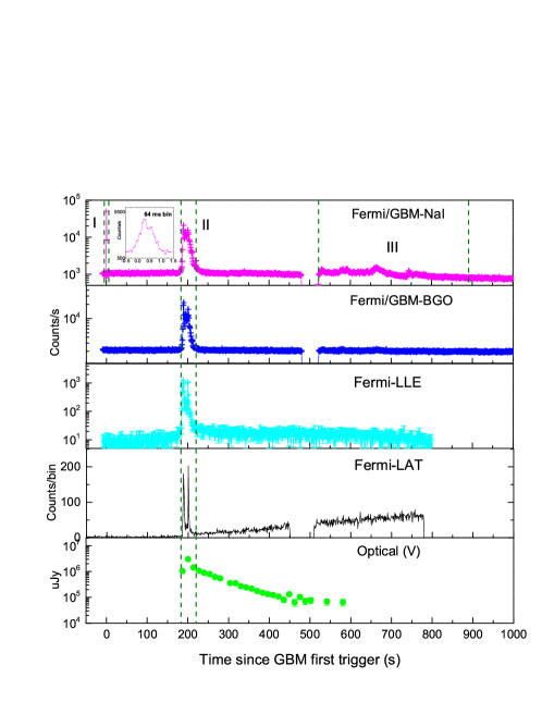
Figure 1: Prompt emission Light curves in different energy bands with one second time-bin. The inset of the top panel shows the temporal structure in 64 milliseconds time-bin. The vertical lines mark the episodes according to the light curve observed with GBM-NaI.

Figure 1 shows the light curves of the prompt and very early optical afterglow emission of GRB 160625B. The GBM-NaI lightcurve has three distinct episodes with 1 second time bin. The first episode lasts about one second (Episode I). The inset in the top panel of Figure 1 shows the lightcurve in 64 ms time-bin. One can find that it is a single pulse with rapidly rising and decaying. It was not detected with GBM-BGO and LAT. The source was in a quiescent stage with a duration of about 180 seconds without detection of any gamma-rays in the GBM and LAT bands. An extremely bright gamma-ray outburst with multiple peaks (Episode II) triggered Fermi-LAT and were also observed with GBM and even in the optical band since $T_{0}+187$ seconds. The source was in quiescent again and triggered GBM at $T_{0}+520$ seconds. The emission in this episode (Episode III) was detected with GBM-NaI detector and LAT. The lightcurve of this episode features as a long-lasting, low flux-level episode, similar to the extended emission (EE) component (e.g., Hu et al. 2014). Its duration is 372 seconds. Therefore, GRB 160625B experiences a short precursor, a main burst, and a long-lasting extended emission stages. The initial three data points of the V band lightcurve of the optical flare observed during the Episode II with the Mini-Mega TORTORA system is very spike. It rapidly increases to the peak brightness ($V=8.04$ magnitude) at $T_{0}+200.3$ seconds with a slope of $\alpha_{1}\sim 20$, then drops with a slope of $\alpha_{2}\sim-15$ after the peak. The optical flux then transits to a decay phase with a slope of $\alpha_{3}\sim-3.41$.

Traditionally, a Band function is invoked to fit the spectra of most GRBs (Band et al. 1993). The physical origin of Band function is interpreted as synchrotron emission of the Poynting-Flux-dominated outflow (Uhm & Zhang 2014; Zhang et al. 2016a). Alternatively, a single black body is invoked to describe the photosphere emission (Rees & Mészáros 2005; Pe’er et al. 2006; Giannios 2008; Beloborodov 2010). In fact, it may be likely from the contributions of various black body radiation, namely, a multi-color blackbody (mBB). Whether the mBB can be composed of black body emission by varying temperature that is still debated. There are many authors to study the photosphere emission from theoretical calculations or numerical simulations by considering several physical effects (e.g., Ryde et al. 2010; Lazzati & Begelman 2010; Pe’er & Ryde 2011; Lundman et al. 2013; Deng & Zhang 2014), but not whole effects. In the framework of the fireball model, the observed spectrum of prompt gamma-rays may be composed of thermal component from the photosphere emission and a non-thermal emission component from the optically thin internal shock region (e.g., Mészáros & Rees 2000). The mBB model can be presented as following that was used in Ryde et al. (2010) and Gao & Zhang (2015), i.e.,

$$F_{\rm mBB}(E,T)=\int^{T_{\rm max}}_{T_{\rm min}}\frac{dA(T)}{dT}\frac{E^{3}}{{\rm exp}[E/kT]-1}~{}dT,$$ (1)

where $T_{\rm max}$ and $T_{\rm mim}$ are free parameters, and $F(T)=\frac{\pi^{4}}{15}A(T)T^{4}$, $A(T)$ is the normalization. We assume that the flux of thermal component is power-law distribution with temperature, which read as

$$F(T)=F_{\rm max}(\frac{T}{T_{\rm max}})^{q},$$ (2)

and $q$ measures the power-law distribution of the temperature. We describe the non-thermal emission component with a cutoff power-law (CPL) model, i.e., $F_{\rm non-th}=F_{0}E^{-\Gamma_{\rm c}}e^{-E/E_{\rm c}}$.

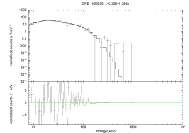
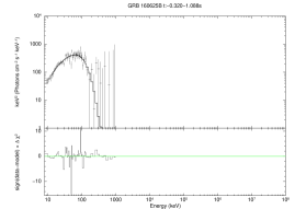
Figure 2: Time-integrated spectrum of the emission Episode I together with our fit by using the mBB model (solid line). Left: count spectrum. Right: $\nu f_{\nu}$ spectrum.

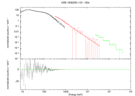
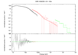
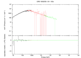
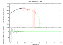
Figure 4: Comparison between the Band function fitting and mBB+CPL model fitting for time-slice [191$\sim$192]. Top two: the observed count spectrum vs. model for Band function fitting (Left) and mBB+CPL fitting (Right). Bottom two: $\nu f_{\nu}$ spectrum plots for Band function fitting (Left) and mBB+CPL fitting (Right). Black, red, and green points are the data observed with NaI, BGO and LAT, respectively.

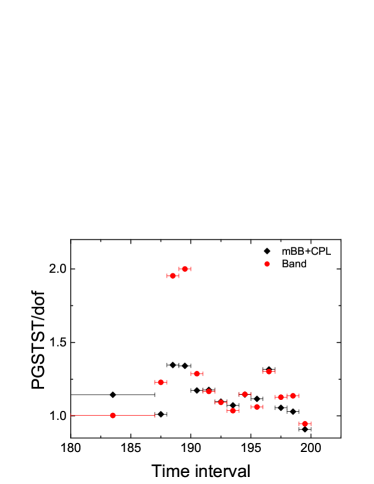
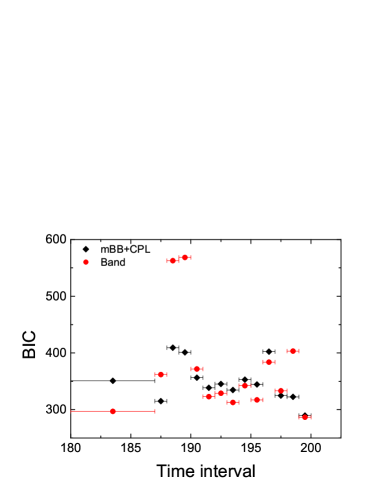
Figure 6: Compare the statistical difference of PGSTST/dof (left) and BIC (right) by using mBB+CPL of Episode II with Band function for each time interval.

We make spectral fit with the Xspec package and evaluate the goodness of our fits with the maximum likelihood-based statistics, so-called PGSTAT (Cash 1979). We jointly analyze the spectra observed with different detectors/telescopes for the first emission episode of the prompt gamma-rays. Figure 2 shows the observed count spectrum and $\nu f_{\nu}$ of Episode I in the GBM energy band. We find that the mBB model is adequate to fit the spectrum of this episode. One has $kT_{\rm max}=25.2\pm 1.1$ keV, $kT_{\rm min}=3.45\pm 1.26$ keV, and $q=0.63\pm 0.2$. For the Episode II, a Band function is also proposed to fit the spectra without considering LAT data (Zhang et al. 2016b; Wang et al. 2017). In this paper, we use the empirical a multi-color blackbody (which motivated by the standard fireball model) plus CPL model to do the time-resolved spectral fit (see Thable 1 and Figure Extremely bright GRB 160625B with multi-episodes emission: Evidences for Long-Term Ejecta Evolution) and get better goodness of fitting. In order to test whether other models can be used to fit the data, we invoke mBB, mBB plus power-law (e.g., GRB 090902B, Ryde et al. 2010) or Band function models to do the spectral fit. We find that the PGSTAT/dof of mBB or mBB plus power-law are too large to be adopted (PGSTAT/dof$>$2), but the Band function is like to be fit the data very well in some time interval. In order to compare the Band function fitting and mBB plus CPL models fitting of Episode II, we give the count and $\nu f_{\nu}$ spectrum for all time-resolved spectra (14 time-slices). Figure 4 shows one example of time-slice ([191$\sim$192] s) for count and $\nu f_{\nu}$ spectrum of those two models. On the other hand, in Figure 6, we compare the goodness of Band function fitting with mBB+CPL fitting, and present the PGSTAT/dof and Bayesian information criterion (BIC) as function of time for each time-slices. From statistical point of view, mBB+CPL model and Band function are comparable between each other.

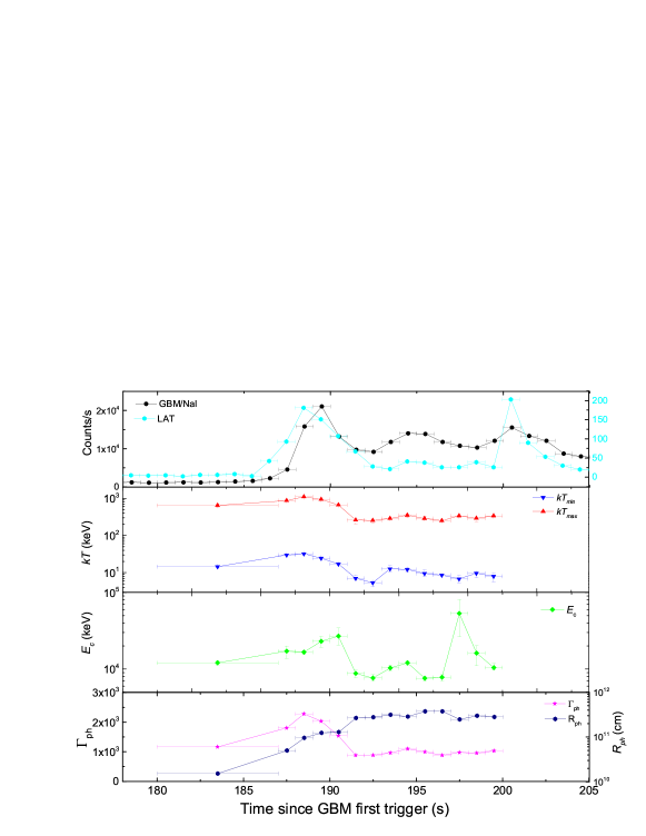
Figure 7: Temporal evolution of $T_{\rm min}$, $T_{\rm max}$, $E_{\rm c}$ and $\Gamma_{\rm ph}$ during Episode II. The top panel is the lightcurves of GBM/NaI and LAT.

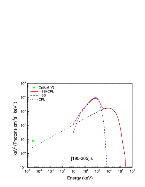
Figure 8: Model curves derived from our fit for the spectrum observed in the time slice [195-205] in comparison with the peak optical flux (the blue dot) in the same time interval, where the optical data is corrected by the extinction of the Milk Way Galaxy and removing the contribution of the reverse shock at this time, but is not corrected for the extinction by the GRB host galaxy.

By invoking mBB plus CPL model to fit the spectra of Episode II, we find that the mBB component is dominated the emission in the range of tens to hundreds of keVs, and both the emission in several keVs and MeVs are attributed from the CPL component. The $kT_{\rm max}$ initially rapidly increases with time from $643\pm 67$ keV to $1096^{+22}_{-23}$ keV, then gradually decays to $250-350$ keV. The power-law index $q$ varies from 0.60 to 1.05. For the CPL component, we do not find any clear temporal evolution feature of $\Gamma_{\rm c}$, which are in the ranges of $\Gamma_{c}\in(1.27,1.69)$. Figure 7 shows the temporal evolution of $kT_{\rm max}$, $kT_{\rm min}$, and $E_{\rm c}$. Note that the bright optical flare was simultaneously detected in the Episode II. It peaks at $T_{0}+\sim 200$ seconds with a exposure time of 10 seconds. We show the model curves derived from our fit for the spectrum observed in the time slice [195-205] seconds in comparison with the peak optical flux in Figure 8. Here, the optical data is corrected by the extinction of the Milk Way Galaxy ($A_{V}=0.349$), but is not corrected for the extinction by the GRB host galaxy due to uncertainly extinction curves. It is found that the optical flux is higher than the model result with a factor of 3. Therefore, it may be contributed by both prompt optical emission and the reverse shocks, as we will discuss below.

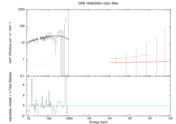
Figure 9: Time-integrated spectrum of the emission Episode III together with our fit by using the CPL+PL model (solid line).

Although the duration of Episode III is longer than Episode II, but its lower flux can not be used to do the time-resolved analysis for this episode. So that, one derive its time-integrated spectrum, which is shown in Figure 9. It is found that the emission in the LAT energy band is dominated by an extra power-law (PL) component. The spectrum cannot be fitted with the mBB+CPL model. Therefore, we use a CPL plus a single PL model to fit the data. One has $\Gamma_{\rm c}=1.64\pm 0.05$, $E_{\rm c}=0.69\pm 0.58$ GeV, and the index of the single PL component is $1.98\pm 0.5$.

3.2 Late Afterglows

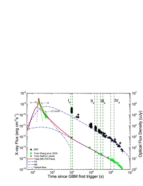
Figure 10: Lightcurves of the prompt optical, early and later optical afterglow, and X-ray afterglow of GRB 160625B. The red line is our model fit with the external shock model, in which the reverse shock and forward shock emission components are represented with the dash-dot-dotted and dash-dotted lines, respectively. The extremely sharp optical pulse of the first three optical data points are suggested to be dominated by the prompt optical flare (black dotted lines). The vertical dashed lines make the selected time slices of our spectral analysis.

Both optical and X-ray afterglows were detected with XRT and UVOT onboard Swift and ground-based telescopes since $T_{0}+10^{4}$ seconds. Their lightcurves show similar features (Figure 10). The later optical afterglow light curve can be well fitted with a smooth broken power-law function, $F=F_{0}[(\frac{t}{t_{b}})^{\omega\alpha_{1}}+(\frac{t}{t_{b}})^{\omega\alpha_{2}}]^{1/\omega}$, and we fixed $\omega=1/3$, which describes the sharpness of the break (Liang et al. 2007). Derived parameters are $\alpha_{\rm O,1}=-0.92\pm 0.04$, $\alpha_{\rm O,2}=-2.30\pm 0.51$, $t_{\rm O,b}=(2.33\pm 0.40)\times 10^{6}$ seconds. The X-ray light curve also can be fitted with this function with parameters $\alpha_{\rm X,1}=-1.31\pm 0.02$, $\alpha_{\rm X,2}=-2.38\pm 0.75$, $t_{\rm X,b}=2.33\times 10^{6}$ seconds (fixed). The achromatic breaks should be due to the jet effect (Rhoads 1997).

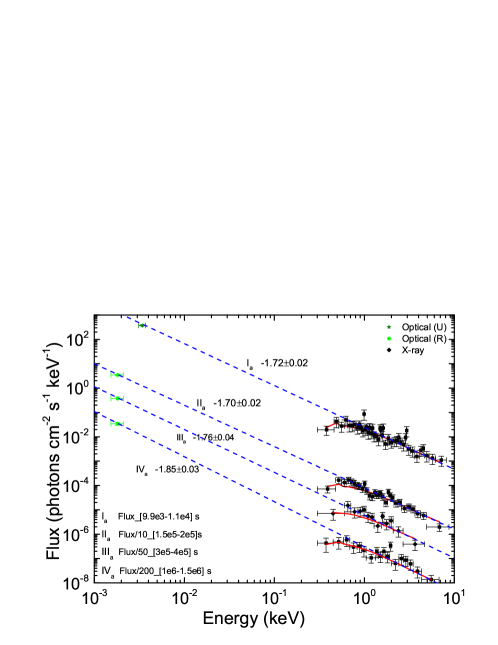
Figure 12: Spectral energy distributions of the Optical-X-ray emission in four selected time intervals. Dashed lines are the spectra fitting with absorbed power-law functions that are extrapolated to the optical bands.

We jointly fit the afterglow spectra in the optical-X-ray band in four selected time slices as marked in Figure 10. By correcting the extinction for the optical data and fixing the neutral hydrogen absorption for the soft X-rays of our Galaxy as $N_{\rm H}=9.76\times 10^{20}$ cm^-2, we find that a single power-law function is adequate to fit the spectra, yielding photon indices $\Gamma=-1.72\pm 0.02$, $-1.70\pm 0.02$, $-1.76\pm 0.04$ and $-1.85\pm 0.03$ for the spectra derived from the four selected time slices. Extinction of the GRB host galaxy is negligible in our fits. Our results are shown in Figure 12. The observed flux slope and the photon index are roughly satisfied with the closure relation $\alpha\sim 3\beta/2$, where $\beta=\Gamma-1$. This suggests that both the X-ray and optical afterglow should be in the spectral regime of $\nu_{m}<\nu<\nu_{c}$, where $\nu_{m}$ and $\nu_{c}$ are the characteristic frequencies of the synchrotron radiation of the relativistic electrons.

4 Derivation of the Ejecta Properties within the Fireball Models

4.1 Lorentz Factor and Radius of the GRB photosphere

Zhang et al (2016b) proposed that the jet composition is dominated from a fireball to a Poynting-flux, and linear polarization during prompt emission were detected (Troja et al. 2017). In our analyses, the time-resolved spectra of Episode II compose of two parts: one is thermal component, and another is non-thermal component (cutoff power-law component). The observed polarization may be contributed from non-thermal component. On the other hand, we assume that the mBB component is from the contributions of photosphere emission. Then, we estimate the $\Gamma_{\rm ph}$ values and radius of the GRB photosphere with the mBB component derived from our spectral fits in different emission episodes. We estimate the $\Gamma_{\rm ph}$ of photosphere emission with Pe’er et al. (2007),

$$\Gamma_{\rm ph}=[(0.16)(1+z)^{2}D_{\rm L}\frac{Y\sigma_{\rm T}F^{\rm obs}}{2m_{\rm p}c^{3}\Re}]^{1/4},$$ (3)

where $D_{\rm L}$ is the luminosity distance, $m_{\rm p}$ is the proton mass, $\sigma_{\rm T}$ is the Thomson scattering cross section, $Y$ is the ratio between total fireball energy and energy radiated in the $\gamma$-ray band, which is fixed at $Y=1$ in our calculation, and $F^{\rm obs}$ is the total observed flux of both the thermal ($F^{\rm obs}_{\rm BB}$) and non-thermal ($F^{\rm obs}_{\rm non-BB}$) components. $\Re$ is defined as

$$\Re=(\frac{F^{\rm obs}_{\rm BB}}{\sigma T^{4}_{\rm max}})^{1/2},$$ (4)

where $F^{\rm obs}_{\rm BB}$ is observed total flux of the mBB component, and $\sigma$ is the Stefan’s constant. The radius of the photosphere can be estimated with

$$R_{\rm ph}=[\frac{\sigma_{T}L_{0}D_{\rm L}^{3}}{8\pi m_{\rm p}c^{3}(1+z)^{6}}(\frac{F_{\rm BB}^{\rm obs}}{\sigma T_{\rm max}^{4}})^{3/2}]^{1/4},$$ (5)

where $L_{0}$ is a total luminosity of both the thermal and non-thermal emission.

The derived $\Gamma_{\rm ph}$ and $R_{\rm ph}$ values are reported in Table 2. It is found that the $\Gamma_{\rm ph}$ value in the Episode I is 175. During Episode II, initially, the $\Gamma_{\rm ph}$ is 1162 in the time slice of [180-187] seconds. Then, it rapidly goes up to 2274 at the time slice of [188-189] seconds, and goes down and keeps at about 800-1100 in the late slices. The $R_{\rm ph}$ value increases from $1.52\times 10^{10}$ cm to $2.66\times 10^{11}$ cm, then keeps in the range of $(2.66-3.76)\times 10^{11}$ cm. The temporal evolution of $\Gamma_{\rm ph}$ and $R_{\rm ph}$ value are shown in bottom panel of Figure 7. The extremely large Lorentz factor may make this event extremely bright (e.g., Liang et al. 2010; Wu et al. 2011).

4.2 Jet Properties Derived from the Afterglow Data

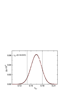
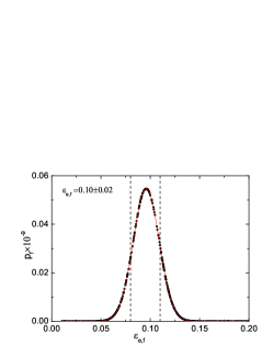
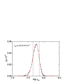
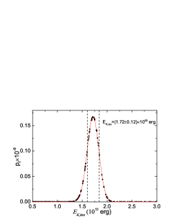
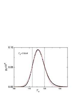
Figure 11: Probability distributions of the afterglow model parameters are well fitted with Gaussian function for GRB 160425B. The dashed vertical lines are marked 1$\sigma$ confidence level of the parameters region.

As mentioned in §3.2, the late afterglow data is consistent with the prediction of the standard afterglow models. We derive the jet properties from the afterglow data in this section. The details of our model and fitting strategy please refer to Huang et al. (2016). With the observed spectral index and temporal decay slope of the normal decay segment (from $10^{5}$ to $10^{6}$ seconds), we suggest that both the optical and X-ray emission should be in the spectral regime between $\nu_{m}$ and $\nu_{c}$, and take $p=2\beta+1\sim 2.4$, where we take $\beta\sim 0.70$ derived from the time slice $[1.5-2.0]\times 10^{5}$ seconds. The fractions of internal energy converted to the electrons and magnetic field are $\varepsilon_{\rm e,r}$ and $\varepsilon_{\rm B,r}$ in the reverse shock region, and $\varepsilon_{\rm e,f}$ and $\varepsilon_{\rm B,f}$ are in the forward shock region. We assume that the medium surrounding the jet is the interstelar medium (ISM) with a constant density ($n$). The temporal evolution of both minimum and cooling frequencies ($\nu_{m}$ and $\nu_{c}$) in the reverse and forward shock regions are taken from Rossi & Rees (2003), Fan & Piran (2006), Zhang et al. (2007) and Yi et al. (2013). We use an Monte Carlo (MC) technique to make the best fit to the observed lightcurves (Xin et al. 2016; Huang et al. 2016), and derive the best parameter set that can reproduce the light curve of observations. A probability $p_{\rm f}=exp(-\chi^{2}/2)$ was invoked to measure the goodness of our fits, where $\chi^{2}$ is reduced $\chi^{2}$. Figure 11 shows the $p_{\rm f}$ distributions along with our Gaussian fits for the best model parameters obtained with our MC technique, and its distributions of those parameters are well fit with Gaussian function, e.g. $\epsilon_{\rm e,r}$, $\epsilon_{\rm e,f}$, $\epsilon_{\rm B,r}$, the fireball kinetic energy $E_{\rm K,iso}$, the initial fireball Lorentz factor $\Gamma_{0}$ and jet opening angle $\theta_{\rm j}$. However, due to the contributions of initial optical flare, the $\epsilon_{\rm B,f}$ and $n$ are not convergent to be fitted by Gaussian function, so we fix those two parameters as $\epsilon_{\rm B,r}\sim 4\times 10^{-5}$ and $n\sim 36\rm~{}cm^{-3}$. For other parameters, one has $\epsilon_{\rm e,r}=0.16\pm 0.02$, $\epsilon_{\rm e,f}=0.1\pm 0.01$, $\epsilon_{\rm B,f}=(1.82\pm 0.47)\times 10^{-7}$, $E_{\rm K,iso}=(1.72\pm 0.12)\times 10^{55}\rm~{}erg$, $\Gamma_{0}=116\pm 4$, $\theta_{\rm j}=12^{\circ}\pm 2^{\circ}$. Defining a magnetization parameter as $R_{B}\equiv\epsilon_{\rm B,r}/\epsilon_{\rm B,f}$, one has $R_{B}\sim 222$. It is lower than that of GRBs 990123, 090102, 130427A and 140512A, whose early optical emission is dominated by the reverse emission (Gao et al. 2015; Huang et al. 2016). Our results are shown in Figure 10. One can observe that the optical emission of the first three data point in the time interval [195, 205] seconds is dominated by a bright optical flare. The segment with a decaying slope of $-3.57\pm 0.09$ is dominated by the reverse shock emission. Late optical and X-ray afterglow since $t>10^{4}$ seconds are contributed by the forward shock emission.

5 Discussion

Three well separated emission episodes observed in GRB 160625B have distinct spectral properties. This may shed light on the evolution of the outflow and even the activity of the GRB central engine. In this section, we discuss possible physical origins of these distinct emission episodes and implications for the central engine of GRB 160625B.

5.1 Episode I: Emission of the Cocoon Surrounding the Jet?

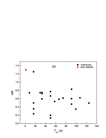
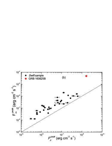
Figure 13: (a): Hardness ratio (HR) as function of precursors duration ($T_{\rm pre}$). (b) Peak flux of main bursts ($F^{\rm peak}_{\rm m}$) as function of Peak flux of precursors ($F^{\rm peak}_{\rm p}$). Black solid circle and red solid star are Swift sample detected precursors and GRB 160625B. The solid line is corresponding to equal peak flux between precursors and main bursts.

Episode I is a short precursor with following long quiescent stage. Hu et al. (2014) made an analysis for a large sample of GRB lightcurves observed with Swift Burst Alert Telescope (BAT) in order to search for the possible precursor emission prior to the main outbursts. They found that about 10% long GRBs have a precursor emission component. Most of precursors show as continuous fluctuations with low flux level. Being due to the narrowness of the BAT band, they fitted the spectra of both the precursors and the main outbursts. They found that their photon indices do not show any statistical difference and suggested that the precursor would be the same emission component from the fireball (see also Lazzati 2005; Burlon et al. 2008). The emission of Episode I of GRB 160625B is dramatically different from these precursors. Its spectrum is well fitted with a mBB model. In addition, it is very short and bright. Figure 13(a) compares Episode I of GRB 160625B with precursors of some Swift GRBs in the plane of the hardness ratio (HR) vs. the duration of the precursors $T_{\rm pre}$, where HR is the ratio of photon fluxes between the 50-100 keV and 15-150 keV bands. It is found that the emission of Episode I is significantly harder than that of the Swift GRBs. The peak fluxes of the precursors of these Swift GRBs are also tightly corrected with that of the main outbursts, but the emission in Episode I deviates this correlation, as shown in Figure 13(b). The peak flux of Episode I of GRB 160625B is much brighter than other Swift GRBs. After the end of Episode I, no signal was detected by GBM and LAT until the Episode II comes. Although tail emission of Episode I may be detectable with Swift/XRT as usually seen in some GRBs (e.g., Peng et al. 2014), the rapid cease of this Episode and a long quiescent stage may indicate the rapid close of this emission channel. Therefore, the physical origin of emission in Episode I may hold the key to reveal the evolution of the GRB jet.

Several models were proposed to interpret the precursor emission of GRBs (Lyutikov & Usov 2000; Ramirez-Ruiz et al. 2002; Wang & Mészáros 2007; Bernardini et al. 2013). It is believed that long GRBs are a relativistic fireball from collapses of massive stars. Lyutikov & Usov (2000) suggested that a weak precursor may attribute to the photosphere emission of the GRB fireball when it becomes transparent. In this scenario, spectrum of the precursor should be thermal or quasi-thermal. Our spectral analysis indicates that the spectrum of Episode I indeed can be fitted with the mBB model. In this scenario, our results likely suggest that the GRB fireball experienced an acceleration stage from Episode I to Epsode II when the fireball was expanded. However, the short duration of Episode I and long quiescent stage after Episode I are difficult to be explained with this scenario since the photosphere emission could not be rapidly shut up when the fireball is transparent.

Ramirez-Ruiz et al. (2002) suggested that a cocoon surrounding a relativistic jet may be formed when the jet breaks out of the progenitor envelope. They assumed that the cocoon has the same Lorentz factor as the GRB jet and discussed possible photospheric “cooling emission” from the cocoon. This emission component may produce gamma-ray and X-ray transients with a short duration since this channel should be rapidly closed due to the drop of pressure. Lazzati et al.(2010) investigated the cocoon evolution and suggested that the transients may be seen similar to a short GRB by an observer at 45^∘. More recently, Nakar & Piran (2017) explored the possible signatures of the cocoon emission. They showed that the cocoon signature depends strongly on the level of mixing between the shocked jet and shocked stellar material. In case of no mixing at all, bright gamma-ray emission with a duration of seconds from the cocoon can be detectable with current missions, such as Swift and Fermi. Non-detection of such an emission component in most GRBs implies that indicates that such kind of mixing must take place. The spectrum and duration of emission in Episode I of GRB 1600625B seem to be consistent with the case of no mixing at all. This makes this GRB very valuable for revealing the progenitor and jet of this GRB (Nakar & Piran 2017).

5.2 Episode II: Main Burst from the Jet?

Our time-resolved spectral analysis for the emission in Episode II shows that the spectra are well fitted with the mBB+CPL model. Lü et al. (2017) present a systematical spectral fit for 37 bright GRBs simultaneously observed with GBM and LAT by invoking the mBB+CPL or mBB+PL models. They show that the spectra of 32 GRBs can be fitted with the mBB+CPL model, and the spectra of other 5 GRBs are adequately fitted with the mBB+PL model. Therefore, the gamma-ray emission of Episode II should be resemble typical LAT GRBs.

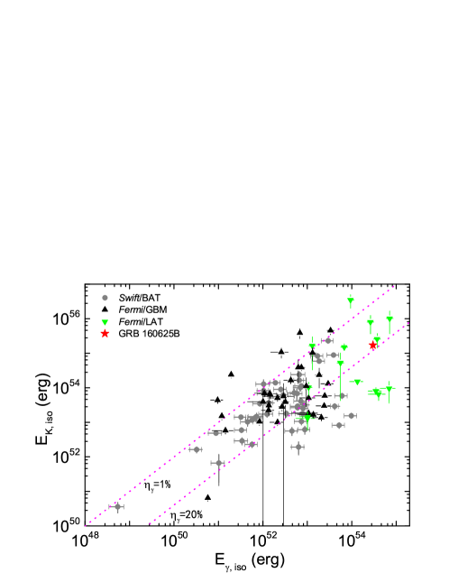
Figure 14: $E_{\rm\gamma,iso}$ as function of $E_{\rm K,iso}$ for Swift/BAT (gray dots), Fermi/GBM (black triangles), Fermi/LAT (green triangles) and GRB 160625B (red star) with redshift measurements (Racusin et al. 2011). The dotted lines mark the constant $\gamma$-ray efficiency ($\eta_{\gamma}$) lines.

A bright optical flare was simultaneously detected in the Episode II. Based on our theoretically modeling with the forward and reverse shock models for the optical and X-ray data as shown in Figure 8, one can find that this flare is shaped by both the prompt optical emission and reverse shock emission, similar to that observed in GRB 140512A (Huang et al. 2016). By subtracting the contribution of the reversed shock emission, the optical flux at the peak time is scaled down a little bit to that extrapolated from the fitting result of the gamma-ray emission. With the derived isotropic kinetic energy from our modeling for the afterglow data and the observed gamma-ray energy of Episode II, we also calculate the GRB radiation efficiency with $\eta_{\gamma}=E_{\rm\gamma,iso}/(E_{\rm\gamma,iso}+E_{\rm K,iso})$ and obtain $\eta_{\gamma}=(14.9\pm 0.9)\%$. We compare the radiation efficiency of GRB 160625B with other GRBs (Racusin et al. 2011). It is also similar to typical long GRBs, as shown in Figure 14.

5.3 Episode III: Extended emission and high energy afterglow emission?

From Figure 1, one can observe that the emission of this episode is clearly detected with GBM-NaI and LAT. The lightcurve observed with NaI features as the extended emission in most GRBs (Hu et al. 2014), but the LAT light curve of this episode steady increase right after the end of the Episode II. The spectrum of Episode III is shown in Figure 9, which also suggests that they should be different emission components. The spectrum observed with LAT should be distinct spectral component from the spectrum observed with GBM. It is well fit with a single power-law with an index of $1.98\pm 0.5$. This component is similar to the extra power-law component observed in GRBs 090902B and 990510 (Ryde et al. 2010; Zhang et al. 2011). We suspect that this component is the high energy afterglows produced in the forward region and the steady increase of the LAT flux could be the onset of the high energy afterglows (e.g., Ghisellini et al. 2010).

6 Conclusions

GRB 160625B is an extremely bright GRB with measured redshift $z=1.406$. The light curve of prompt emission is composed of three distinct episodes: a short precursor (Episode I), a very bright main emission episode (Episode II), and a weak emission episode, (Episode III). Those three episodes emission are separated by two quiet period of $\sim 180$ and $\sim 300$ seconds, respectively. The total isotropic-equivalent energy ($E_{\gamma,iso}$) and peak luminosity ($L_{\rm iso}$) are as high as $\sim 3\times 10^{54}$ erg and $\sim 4\times 10^{53}\rm~{}erg~{}s^{-1}$, respectively. The early optical emission is very bright with 8.04 magnitude during the main emission episode. By analyzing its data observed with the GBM and LAT on board the Fermi mission, we find the following interesting results:

• The emission of Episode I is significantly harder than that of the Swift GRBs. The spectrum of Episode I can be fitted with a mBB model, and the derived maximum temperature ($kT_{\rm max}$) is $\sim 25$ keV. Those features suggest that the Episode I is different from other Swift GRBs detected precursors. We propose that the emission of Episode I seems to be from the emission of cocoon surrounding the jet with the case of no mixing between shocked jet cocoon and shocked stellar cocoon.

• An extremely bright of Episode II has a higher isotropic-equivalent energy, and the time-resolved spectral analysis for the emission in Episode II shows that the spectra are well fitted with a model composing of an mBB component plus a cutoff power-law component. The radiation efficiency of this Episode is similar to other typical long GRBs. Those features suggest that the emission of Episode II is contributed by both photosphere emission and internal shock of relativistic jet. However, the Poynting-Flux-dominated outflow can not be ruled out only based on data itself.

• The spectrum of Episode III is adequately fitted with a CPL plus a single power-law models, and no mBB component is required. This may imply that the emission Episode III is contributed by both internal and external shocks of relativistic jet.

• The early and later afterglows are consistent with reverse and forward shock models, respectively. Derived the initial fireball Lorentz factor $\Gamma_{0}=116\pm 4$, and jet opening angle $\theta_{\rm j}=12^{\circ}\pm 2^{\circ}$.

Although, the empirical function of multi-color black body can be used to fit the observed data very well. However, the physical meaning of mBB is still unclear, especially, the parameter $q$ of this model which is varying with time. More important observations are expected in the future to explore the physical meaning of mBB, or through theoretical study and numerical simulations.

Table 1: Time-resolved Spectral fitting with mBB+CPL and Band models for Episode II of GRB 160625B

Time interval		mBB		CPL		$\rm PGS/{\rm dof}$		Band		$\rm PGS/{\rm dof}$	$\Delta\rm BIC$	BIC-selected model
(s)	$kT_{\rm min}$ (keV)	$kT_{\rm max}$ (keV)	$q$	$\Gamma_{c}$	$E_{\rm c}$ (MeV)		$\hat{\alpha}$	$\hat{\beta}$	$E_{\rm p}$ (keV)
[$180\sim 187$] (catalog )	15 ${}_{-1.20}^{+1.20}$	643${}_{-68}^{+68}$	0.90 ${}_{-0.04}^{+0.04}$	1.27 ${}_{-0.02}^{+0.02}$	12.11 ${}_{-0.83}^{+0.83}$	310/271	$-0.89\pm 0.02$	-4.22${}_{-1.76}^{+0.51}$	$5855_{-644}^{+1298}$	275/274	-54	Band(very strong)
[$187\sim 188$] (catalog )	30 ${}_{-0.68}^{+0.26}$	871 ${}_{-27}^{+49}$	0.81 ${}_{-0.02}^{+0.03}$	1.31 ${}_{-0.01}^{+0.02}$	17.19 ${}_{-2.86}^{+3.40}$	276/273	$-0.96\pm 0.03$	-2.85 ${}_{-0.05}^{+0.11}$	$2999_{-273}^{+521}$	339/276	47	mBB+CPL(very strong)
[$188\sim 189$] (catalog )	32 ${}_{-0.36}^{+0.38}$	1096 ${}_{-23}^{+22}$	0.64 ${}_{-0.01}^{+0.02}$	1.34 ${}_{-0.01}^{+0.02}$	16.59 ${}_{-0.71}^{+1.03}$	369/274	$-0.77\pm 0.02$	$-2.64\pm 0.03$	$1294_{-87}^{+92}$	541/277	153	mBB+CPL(very strong)
[$189\sim 190$] (catalog )	25 ${}_{-0.48}^{+0.48}$	940 ${}_{-20}^{+40}$	0.60 ${}_{-0.02}^{+0.02}$	1.50 ${}_{-0.03}^{+0.02}$	23.09 ${}_{-3.63}^{+3.78}$	362/270	$-0.75\pm 0.03$	$-2.62\pm 0.02$	$813_{-51}^{+56}$	546/273	167	mBB+CPL(very strong)
[$190\sim 191$] (catalog )	17 ${}_{-1.36}^{+0.29}$	659 ${}_{-66}^{+7}$	0.59 ${}_{-0.02}^{+0.02}$	1.60 ${}_{-0.02}^{+0.04}$	26.97 ${}_{-7.36}^{+6.40}$	318/271	$-0.81\pm 0.03$	$-2.58\pm 0.04$	$624_{-49}^{+60}$	354/275	15	mBB+CPL(very strong)
[$191\sim 192$] (catalog )	7 ${}_{-1.44}^{+0.69}$	260 ${}_{-25}^{+56}$	0.68 ${}_{-0.01}^{+0.01}$	1.52 ${}_{-0.02}^{+0.02}$	8.75 ${}_{-0.95}^{+0.96}$	299/254	$-0.81\pm 0.05$	$-2.70\pm 0.07$	$364_{-40}^{+40}$	300/257	-16	Band(very strong)
[$192\sim 193$] (catalog )	5 ${}_{-0.73}^{+1.25}$	254 ${}_{-18}^{+41}$	0.72 ${}_{-0.01}^{+0.01}$	1.47 ${}_{-0.01}^{+0.02}$	7.64 ${}_{-0.84}^{+0.69}$	305/278	$-0.81\pm 0.05$	$-2.70\pm 0.08$	$366_{-38}^{+40}$	307/281	-16	Band(very strong)
[$193\sim 194$] (catalog )	13 ${}_{-2.53}^{+2.09}$	289 ${}_{-26}^{+18}$	0.92 ${}_{-0.04}^{+0.02}$	1.50 ${}_{-0.01}^{+0.01}$	10.35 ${}_{-0.85}^{+0.96}$	296/276	$-0.70\pm 0.04$	$-2.78\pm 0.06$	$416_{-30}^{+36}$	289/279	-22	Band(very strong)
[$194\sim 195$] (catalog )	12 ${}_{-1.37}^{+1.62}$	350 ${}_{-27}^{+34}$	0.86 ${}_{-0.03}^{+0.06}$	1.53 ${}_{-0.08}^{+0.02}$	12.07 ${}_{-0.91}^{+1.01}$	315/275	$-0.74\pm 0.03$	$-2.80\pm 0.05$	$504_{-32}^{+38}$	319/278	-11	Band(very strong)
[$195\sim 196$] (catalog )	10 ${}_{-2.18}^{+1.57}$	287 ${}_{-36}^{+25}$	1.02 ${}_{-0.08}^{+0.02}$	1.38 ${}_{-0.03}^{+0.02}$	7.60 ${}_{-0.49}^{+0.61}$	307/275	$-0.72\pm 0.03$	$-2.88\pm 0.07$	$467_{-29}^{+35}$	295/278	-27	Band(very strong)
[$196\sim 197$] (catalog )	9 ${}_{-0.04}^{+0.04}$	252 ${}_{-7}^{+4}$	1.01 ${}_{-0.01}^{+0.01}$	1.40 ${}_{-0.02}^{+0.02}$	7.79 ${}_{-0.65}^{+0.86}$	362/275	$-0.74\pm 0.04$	$-2.89\pm 0.08$	$418_{-29}^{+34}$	362/278	-18	Band(very strong)
[$197\sim 198$] (catalog )	7 ${}_{-1.43}^{+1.49}$	338 ${}_{-22}^{+27}$	0.94 ${}_{-0.05}^{+0.05}$	1.69 ${}_{-0.08}^{+0.17}$	53.48 ${}_{-26.89}^{+78.94}$	287/272	$-0.78\pm 0.03$	$-3.08\pm 0.10$	$525_{-36}^{+47}$	310/275	8	mBB+CPL(strong)
[$198\sim 199$] (catalog )	10 ${}_{-1.10}^{+2.14}$	292 ${}_{-6}^{+52}$	0.98 ${}_{-0.03}^{+0.01}$	1.54 ${}_{-0.04}^{+0.05}$	16.11 ${}_{-4.08}^{+5.05}$	283/275	$-0.78\pm 0.03$	$-2.71\pm 0.05$	$492_{-39}^{+49}$	316/278	81	mBB+CPL(very strong)
[$199\sim 200$] (catalog )	8 ${}_{-1.63}^{+2.28}$	338 ${}_{-20}^{+34}$	1.05 ${}_{-0.06}^{+0.06}$	1.51 ${}_{-0.06}^{+0.09}$	10.44 ${}_{-1.36}^{+0.67}$	250/275	$-0.75\pm 0.03$	$-3.02\pm 0.08$	$578_{-42}^{+42}$	263/278	3	mBB+CPL(positive)

Table 2: The Derived Properties of the Episodes II

Time Interval (s)	$F^{\rm obs}_{\rm BB}$	$F^{\rm obs}_{\rm non-BB}$	$\Gamma_{\rm ph}$	$R_{\rm ph}$
[$180\sim 187$] (catalog )	0.11	0.22	1162	0.15
[$187\sim 188$] (catalog )	1.54	2.41	1798	0.50
[$188\sim 189$] (catalog )	8.98	6.42	2274	0.96
[$189\sim 190$] (catalog )	10.11	4.19	2035	1.24
[$190\sim 191$] (catalog )	4.64	1.81	1540	1.29
[$191\sim 192$] (catalog )	1.45	0.99	878	2.66
[$192\sim 193$] (catalog )	1.43	1.13	879	2.78
[$193\sim 194$] (catalog )	2.57	1.19	959	3.13
[$194\sim 195$] (catalog )	3.57	1.55	1095	2.87
[$195\sim 196$] (catalog )	3.37	1.62	992	3.76
[$196\sim 197$] (catalog )	2.49	1.01	883	3.74
[$197\sim 198$] (catalog )	2.93	0.20	975	2.48
[$198\sim 199$] (catalog )	2.47	1.05	953	2.98
[$199\sim 200$] (catalog )	3.39	0.76	1028	2.81

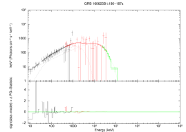
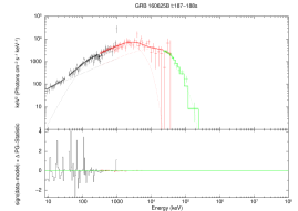
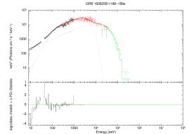
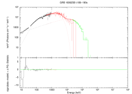
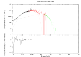
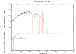
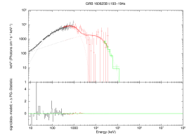
Figure 3: Observed time-resolved $\nu F_{\nu}$ spectra of the emission Episode II (the main emission episode) together with our fits with the mBB+CPL model (dot lines). Black points, red points, and green points are data observed with NaI, BGO and LAT, respectively.

Fig.3—continued.

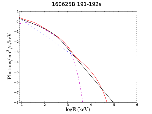
Figure 5: Comparison photon models between Band function (black solid line) and mBB (dot pink line) with CPL (dot blue line) in Figure 4. The red solid line is the superposition of mBB and CPL models.

References

- Band et al. (1993) Band, D., Matteson, J., Ford, L., et al. 1993, ApJ, 413, 281
- Beloborodov (2010) Beloborodov, A. M. 2010, MNRAS, 407, 1033
- Bernardini et al. (2013) Bernardini, M. G., Campana, S., Ghisellini, G., et al. 2013, ApJ, 775, 67
- Burlon et al. (2008) Burlon, D., Ghirlanda, G., Ghisellini, G., et al. 2008, ApJ, 685, L19
- Burns (2016) Burns, E. 2016, GRB Coordinates Network, 19581, 1
- Cash (1979) Cash, W. 1979, ApJ, 228, 939
- Dai & Lu (1998) Dai, Z. G., & Lu, T. 1998, A&A, 333, L87
- Deng & Zhang (2014) Deng, W., & Zhang, B. 2014, ApJ, 785, 112
- Dirirsa et al. (2016) Dirirsa, F., Vianello, G., Racusin, J., & Axelsson, M. 2016, GRB Coordinates Network, 19586, 1
- Fan & Piran (2006) Fan, Y., & Piran, T. 2006, MNRAS, 369, 197
- Fruchter et al. (2006) Fruchter, A. S., Levan, A. J., Strolger, L., et al. 2006, Nature, 441, 463
- Fraija et al. (2017) Fraija, N., Veres, P., Zhang, B. B., et al. 2017, arXiv:1705.09311
- Galama et al. (1998) Galama, T. J., Vreeswijk, P. M., van Paradijs, J., et al. 1998, Nature, 395, 670
- Gao et al. (2013) Gao, H., Lei, W.-H., Zou, Y.-C., Wu, X.-F., & Zhang, B. 2013, NewAR, 57, 141
- Gao et al. (2015) Gao, H., Wang, X.-G., Mészáros, P., & Zhang, B. 2015, ApJ, 810, 160
- Gao & Zhang (2015) Gao, H., & Zhang, B. 2015, ApJ, 801, 103
- Geng et al. (2016) Geng, J.-J., Zhang, B., & Kuiper, R. 2016, ApJ, 833, 116
- Ghisellini et al. (2010) Ghisellini, G., Ghirlanda, G., Nava, L., & Celotti, A. 2010, MNRAS, 403, 926
- Ghisellini et al. (2007) Ghisellini, G., Ghirlanda, G., & Tavecchio, F. 2007, MNRAS, 375, L36
- Giannios (2008) Giannios, D. 2008, A&A, 480, 305
- Hu et al. (2014) Hu, Y.-D., Liang, E.-W., Xi, S.-Q., et al. 2014, ApJ, 789, 145
- Huang et al. (2016) Huang, X.-L., Xin, L.-P., Yi, S.-X., et al. 2016, ApJ, 833, 100
- Lü & Zhang (2014) Lü, H.-J., & Zhang, B. 2014, ApJ, 785, 74
- Lü et al. (2017) Lü et al. 2017, in preparation.
- Lazzati (2005) Lazzati, D. 2005, MNRAS, 357, 722
- Lazzati & Begelman (2010) Lazzati, D., & Begelman, M. C. 2010, ApJ, 725, 1137
- Lazzati & Begelman (2005) Lazzati, D., & Begelman, M. C. 2005, ApJ, 629, 903
- Lazzati et al. (2010) Lazzati, D., Morsony, B. J., & Begelman, M. C. 2010, ApJ, 717, 239
- Lei et al. (2013) Lei, W.-H., Zhang, B., & Liang, E.-W. 2013, ApJ, 765, 125
- Liang et al. (2010) Liang, E.-W., Yi, S.-X., Zhang, J., et al. 2010, ApJ, 725, 2209
- Liang et al. (2007) Liang, E.-W., Zhang, B.-B., & Zhang, B. 2007, ApJ, 670, 565
- Lundman et al. (2013) Lundman, C., Pe’er, A., & Ryde, F. 2013, MNRAS, 428, 2430
- Lyutikov & Usov (2000) Lyutikov, M., & Usov, V. V. 2000, ApJ, 543, L129
- Mészáros & Rees (2000) Mészáros, P., & Rees, M. J. 2000, ApJ, 530, 292
- Mészáros & Rees (1997) Mészáros, P., & Rees, M. J. 1997, ApJ, 476, 232
- Meegan et al. (2009) Meegan, C., Lichti, G., Bhat, P. N., et al. 2009, ApJ, 702, 791-804
- Melandri et al. (2016) Melandri, A., D’Avanzo, P., D’Elia, V., et al. 2016, GRB Coordinates Network, 19585, 1
- Meszaros & Rees (1993) Meszaros, P., & Rees, M. J. 1993, ApJ, 405, 278
- Mizuta & Ioka (2013) Mizuta, A., & Ioka, K. 2013, ApJ, 777, 162
- Morsony et al. (2007) Morsony, B. J., Lazzati, D., & Begelman, M. C. 2007, ApJ, 665, 569
- Nakar & Piran (2017) Nakar, E., & Piran, T. 2017, ApJ, 834, 28
- Narayan et al. (2001) Narayan, R., Piran, T., & Kumar, P. 2001, ApJ, 557, 949
- Paczyński (1998) Paczyński, B. 1998, ApJ, 494, L45
- Pe’er et al. (2006) Pe’er, A., Mészáros, P., & Rees, M. J. 2006, ApJ, 642, 995
- Pe’er & Ryde (2011) Pe’er, A., & Ryde, F. 2011, ApJ, 732, 49
- Pe’er et al. (2007) Pe’er, A., Ryde, F., Wijers, R. A. M. J., Mészáros, P., & Rees, M. J. 2007, ApJ, 664, L1
- Peng et al. (2014) Peng, F.-K., Liang, E.-W., Wang, X.-Y., et al. 2014, ApJ, 795, 155
- Piran et al. (1993) Piran, T., Shemi, A., & Narayan, R. 1993, MNRAS, 263, 861
- Piro et al. (2014) Piro, L., Troja, E., Gendre, B., et al. 2014, ApJ, 790, L15
- Popham et al. (1999) Popham, R., Woosley, S. E., & Fryer, C. 1999, ApJ, 518, 356
- Racusin et al. (2011) Racusin, J. L., Oates, S. R., Schady, P., et al. 2011, ApJ, 738, 138
- Ramirez-Ruiz et al. (2002) Ramirez-Ruiz, E., Celotti, A., & Rees, M. J. 2002, MNRAS, 337, 1349
- Rees & Mészáros (2005) Rees, M. J., & Mészáros, P. 2005, ApJ, 628, 847
- Rees & Meszaros (1994) Rees, M. J., & Meszaros, P. 1994, ApJ, 430, L93
- Rhoads (1997) Rhoads, J. E. 1997, ApJ, 487, L1
- Rossi & Rees (2003) Rossi, E., & Rees, M. J. 2003, MNRAS, 339, 881
- Ryde et al. (2010) Ryde, F., Axelsson, M., Zhang, B. B., et al. 2010, ApJ, 709, L172
- Sari et al. (1998) Sari, R., Piran, T., & Narayan, R. 1998, ApJ, 497, L17
- Stanek et al. (2003) Stanek, K. Z., Matheson, T., Garnavich, P. M., et al. 2003, ApJ, 591, L17
- Svinkin et al. (2016) Svinkin, D., Golenetskii, S., Aptekar, R., et al. 2016, GRB Coordinates Network, 19604, 1
- Thompson (1994) Thompson, C. 1994, MNRAS, 270, 480
- Troja et al. (2010) Troja, E., Rosswog, S., & Gehrels, N. 2010, ApJ, 723, 1711
- Troja et al. (2017) Troja, E., Lipunov, V. M., Mundell, C.G., et al. 2017, Nature, 547, 425
- Uhm & Zhang (2014) Uhm, Z. L., & Zhang, B. 2014, Nature Physics, 10, 351
- Usov (1992) Usov, V. V. 1992, Nature, 357, 472
- Wang & Mészáros (2007) Wang, X.-Y., & Mészáros, P. 2007, ApJ, 670, 1247
- Wang et al. (2017) Wang, Y.-Z., Wang, H., Zhang, S., et al. 2017, ApJ, 836, 81
- Woosley (1993) Woosley, S. E. 1993, ApJ, 405, 273
- Woosley & Bloom (2006) Woosley, S. E., & Bloom, J. S. 2006, ARA&A, 44, 507
- Wu et al. (2011) Wu, Q., Zou, Y.-C., Cao, X., Wang, D.-X., & Chen, L. 2011, ApJ, 740, L21
- Xin et al. (2016) Xin, L.-P., Wang, Y.-Z., Lin, T.-T., et al. 2016, ApJ, 817, 152
- Xu et al. (2016) Xu, D., Malesani, D., Fynbo, J. P. U., et al. 2016, GRB Coordinates Network, 19600, 1
- Yi et al. (2013) Yi, S.-X., Wu, X.-F., & Dai, Z.-G. 2013, ApJ, 776, 120
- Zhang et al. (2016) Zhang, B.-B., Uhm, Z. L., Connaughton, V., Briggs, M. S., & Zhang, B. 2016a, ApJ, 816, 72
- Zhang et al. (2016) Zhang, B.-B., Zhang, B., Castro-Tirado, A. J., et al. 2016b, arXiv:1612.03089
- Zhang et al. (2011) Zhang, B.-B., Zhang, B., Liang, E.-W., et al. 2011, ApJ, 730, 141
- Zhang & Kobayashi (2005) Zhang, B., & Kobayashi, S. 2005, ApJ, 628, 315
- Zhang et al. (2007) Zhang, B., Liang, E., Page, K. L., et al. 2007, ApJ, 655, 989
- Zhang & Yan (2011) Zhang, B., & Yan, H. 2011, ApJ, 726, 90
- Zhang et al. (2003) Zhang, W., Woosley, S. E., & MacFadyen, A. I. 2003, ApJ, 586, 356