Abstract

Many contemporary statistical learning methods assume a Euclidean feature space. This paper presents a method for defining similarity based on hyperspherical geometry and shows that it often improves the performance of support vector machine compared to other competing similarity measures. Specifically, the idea of using heat diffusion on a hypersphere to measure similarity has been previously proposed and tested by [1], demonstrating promising results based on a heuristic heat kernel obtained from the zeroth order parametrix expansion; however, how well this heuristic kernel agrees with the exact hyperspherical heat kernel remains unknown. This paper presents a higher order parametrix expansion of the heat kernel on a unit hypersphere and discusses several problems associated with this expansion method. We then compare the heuristic kernel with an exact form of the heat kernel expressed in terms of a uniformly and absolutely convergent series in high-dimensional angular momentum eigenmodes. Being a natural measure of similarity between sample points dwelling on a hypersphere, the exact kernel often shows superior performance in kernel SVM classifications applied to text mining, tumor somatic mutation imputation, and stock market analysis.

1 Introduction

As the techniques for analyzing large data sets continue to grow, diverse quantitative sciences – including computational biology, observation astronomy, and high energy physics – are becoming increasingly data driven. Moreover, modern business decision making critically depends on quantitative analyses such as community detection and consumer behavior prediction. Consequently, statistical learning has become an indispensable tool for modern data analysis. Data acquired from various experiments are usually organized into an $n\times m$ matrix, where the number $n$ of features typically far exceeds the number $m$ of samples. In this view, the $m$ samples, corresponding to the columns of the data matrix, are naturally interpreted as points in a high-dimensional feature space $\mathbb{R}^{n}$. Traditional statistical modeling approaches often lose their power when the feature dimension is high. To ameliorate this problem, Lafferty and Lebanon proposed a multinomial interpretation of non-negative feature vectors and an accompanying transformation of the multinomial simplex to a hypersphere, demonstrating that using the heat kernel on this hypersphere may improve the performance of kernel support vector machine (SVM) [1, 2, 3, 4, 5, 6, 7]. Despite the interest that this idea has attracted, only approximate heat kernel is known to date. We here present an exact form of the heat kernel on a hypersphere of arbitrary dimension and study its performance in kernel SVM classifications of text mining, genomic, and stock price data sets.

To date, sparse data clouds have been extensively analyzed in the flat Euclidean space endowed with the $L^{2}$-norm using traditional statistical learning algorithms, including KMeans, hierarchical clustering, SVM, and neural network [2, 8, 3, 4, 5, 6, 7]; however, the flat geometry of the Euclidean space often poses severe challenges in clustering and classification problems when the data clouds take non-trivial geometric shapes or class labels are spatially mixed. Manifold learning and kernel-based embedding methods attempt to address these challenges by estimating the intrinsic geometry of a putative submanifold from which the data points were sampled and by embedding the data into an abstract Hilbert space using a nonlinear map implicitly induced by the chosen kernel, respectively [9, 10, 11]. The geometry of these curved spaces may then provide novel information about the structure and organization of original data points.

Heat equation on the data submanifold or transformed feature space offers an especially attractive idea of measuring similarity between data points by using the physical model of diffusion of relatedness (“heat”) on curved space, where the diffusion process is driven by the intrinsic geometry of the underlying space. Even though such diffusion process has been successfully approximated as a discrete-time, discrete-space random walk on complex networks, its continuous formulation is rarely analytically solvable and usually requires complicated asymptotic expansion techniques from differential geometry [12]. An analytic solution, if available, would thus provide a valuable opportunity for comparing its performance with approximate asymptotic solutions and rigorously testing the power of heat diffusion for geometric data analysis.

Given that a Riemannian manifold of dimension $d$ is locally homeomorphic to $\mathbb{R}^{d}$, and that the heat kernel is a solution to the heat equation with a point source initial condition, one may assume in the short diffusion time limit ($t\downarrow 0$) that most of the heat is localized within the vicinity of the initial point and that the heat kernel on a Riemannian manifold locally resembles the Euclidean heat kernel. This idea forms the motivation behind the parametrix expansion, where the heat kernel in curved space is approximated as a product of the Euclidean heat kernel in normal coordinates and an asymptotic series involving the diffusion time and normal coordinates. In particular, for a unit hypersphere, the parametrix expansion in the limit $t\downarrow 0$ involves a modified Euclidean heat kernel with the Euclidean distance $\left\|\mathbf{x}\right\|$ replaced by the geodesic arc length $\theta$. Computing this parametrix expansion is, however, technically challenging; even when the computation is tractable, applying the approximation directly to high-dimensional clustering and classification problems may have limitations. For example, in order to be able to group samples robustly, one needs the diffusion time $t$ to be not too small; otherwise, the sample relatedness may be highly localized and decay too fast away from each sample. Moreover, the leading order term in the asymptotic series is an increasing function of $\theta$ and diverges as $\theta$ approaches $\pi$, yielding an incorrect conclusion that two antipodal points are highly similar. For these reasons, the machine learning community has been using only the Euclidean diffusion term without the asymptotic series correction; how this resulting kernel, called the parametrix kernel [1], compares with the exact heat kernel on a hypersphere remains an outstanding question, which is addressed in this paper.

Analytically solving the diffusion equation on a Riemannian manifold is challenging [13, 14, 12]. Unlike the discrete analogues – such as spectral clustering [15] and diffusion map [16], where eigenvectors of a finite dimensional matrix can be easily obtained – the eigenfunctions of the Laplace operator on a Riemannian manifold are usually intractable. Fortunately, the high degree of symmetry of a hypersphere allows the explicit construction of eigenfunctions, called hyperspherical harmonics, via the projection of homogeneous polynomials [17, 18]. The exact heat kernel is then obtained as a convergent power series in these eigenfunctions. In this paper, we compare the analytic behavior of this exact heat kernel with that of the parametrix kernel and analyze their performance in classification.

2 Results

The heat kernel is the fundamental solution to the heat equation $(\partial_{t}-\Delta_{x})u(x,t)=0$ with an initial point source [19], where $\Delta_{x}$ is the Laplace operator; the amount of heat emanating from the source that has diffused to a neighborhood during time $t>0$ is used to measure the similarity between the source and proximal points. The heat conduction depends on the geometry of feature space, and the main idea behind the application of hyperspherical geometry to data analysis relies on the following map from a non-negative feature space to a unit hypersphere:

Definition 1

A hyperspherical map $\varphi:\mathbb{R}_{\geq 0}^{n}\setminus\{0\}\rightarrow S^{n-1}$ maps a vector $\mathbf{x}$, with $x_{i}\geq 0$ and $\sum_{i=1}^{n}x_{i}>0$, to a unit vector $\hat{x}\in S^{n-1}$ where $(\hat{x})_{i}\equiv\sqrt{x_{i}/\sum_{j=1}^{n}x_{j}}$.

We will henceforth denote the image of a feature vector $\mathbf{x}$ under the hyperspherical map as $\hat{x}$. The notion of neighborhood requires a well-defined measurement of distance on the hypersphere, which is naturally the great arc length – the geodesic on a hypersphere. Both parametrix approximation and exact solution employ the great arc length, which is related to the following definition of cosine similarity:

Definition 2

The generic cosine similarity between two feature vectors $\mathbf{x},\mathbf{y}\in\mathbb{R}^{n}\setminus\{0\}$ is

$$\cos\theta\equiv\frac{\mathbf{x}\cdot\mathbf{y}}{\left\|\mathbf{x}\right\|\left\|\mathbf{y}\right\|},$$

where $\left\|\cdot\right\|$ is the Euclidean $L^{2}$-norm, and $\theta\in[0,\pi]$ is the great arc length on $S^{n-1}$. For unit vectors $\hat{x}=\varphi(\mathbf{x})$ and $\hat{y}=\varphi(\mathbf{y})$ obtained from non-negative feature vectors $\mathbf{x},\mathbf{y}\in\mathbb{R}_{\geq 0}^{n}\setminus\{0\}$ via the hyperspherical map, the cosine similarity reduces to the dot product $\cos\theta=\hat{x}\cdot\hat{y}$; the non-negativity of $\bf x$ and $\bf y$ guarantees that $\theta\in[0,\pi/2]$ in this case.

2.1 Parametrix expansion

The parametrix kernel $K^{{\rm prx}}$ previously used in the literature is just a Gaussian RBF function with $\theta=\arccos\hat{x}\cdot\hat{y}$ as the radial distance [1]:

Definition 3

The parametrix kernel is a non-negative function

$$K^{{\rm prx}}(\hat{x},\hat{y};t)={\rm e}^{-\frac{\arccos^{2}\hat{x}\cdot\hat{y}}{4t}}={\rm e}^{-\frac{\theta^{2}}{4t}},$$

defined for $t>0$ and attaining global maximum $1$ at $\theta=0$.

Note that this kernel is assumed to be restricted to the positive orthant. The normalization factor $(4\pi t)^{-\frac{n-1}{2}}$ is numerically unstable as $t\downarrow 0$ and complicates hyperparameter tuning; as a global scaling factor of the kernel can be absorbed into the misclassification $C$-parameter in SVM, this overall normalization term is ignored in this paper. Importantly, the parametrix kernel $K^{{\rm prx}}$ is merely the Gaussian multiplicative factor without any asymptotic expansion terms in the full parametrix expansion $G^{{\rm prx}}$ of the heat kernel on a hypersphere [1, 12], as described below.

The Laplace operator on manifold $\mathcal{M}$ equiped with a Riemannian metric $g_{\mu\nu}$ acts on a function $f$ that depends only on the geodesic distance $r$ from a fixed point as

$$\Delta f(r)=f^{\prime\prime}(r)+\left(\log\sqrt{g}\right)^{\prime}f^{\prime}(r),$$ (1)

where $g\equiv\det(g_{\mu\nu})$ and ^′ denotes the radial derivative. Due to the nonvanishing metric derivative in Equation 1, the canonical diffusion function

$$G(r,t)=\left(\frac{1}{4\pi t}\right)^{\frac{d}{2}}\exp\left(-\frac{r^{2}}{4t}\right)$$ (2)

does not satisfy the heat equation; that is, $(\Delta-\partial_{t})G(r,t)\neq 0$ (Supplementary Material, Section S2). For sufficiently small time $t$ and geodesic distance $r$, the parametrix expansion of the heat kernel on a full hypersphere proposes an approximate solution

$$K_{p}(r,t)=G(r,t)\left(u_{0}(r)+u_{1}(r)t+u_{2}(r)t^{2}+\cdots+u_{p}(r)t^{p}\right),$$

where the functions $u_{i}$ should be found such that $K_{p}$ satisfies the heat equation to order $t^{p-d/2}$, which is small for $t\ll 1$ and $p>d/2$; more precisely, we seek $u_{i}$ such that

$$(\Delta-\partial_{t})K_{p}=G\,t^{p}\,\Delta u_{p}.$$ (3)

Taking the time derivative of $K_{p}$ yields

$$\partial_{t}K_{p}=G\cdot\left[\left(-\frac{d}{2t}+\frac{r^{2}}{4t^{2}}\right)\left(u_{0}+u_{1}t+u_{2}t^{2}+\cdots+u_{p}t^{p}\right)+\left(u_{1}+2u_{2}t+\cdots+pu_{p}t^{p-1}\right)\right],$$

while the Laplacian of $K_{p}$ is

$$\Delta K_{p}=\left(u_{0}+u_{1}t+\cdots+u_{p}t^{p}\right)\Delta G+G\Delta\left(u_{0}+u_{1}t+\cdots+u_{p}t^{p}\right)+2G^{\prime}\left(u_{0}+u_{1}t+\cdots+u_{p}t^{p}\right)^{\prime}.$$

One can easily compute

$$\Delta G=\left[\left(-\frac{1}{2t}+\frac{r^{2}}{4t^{2}}\right)-\frac{r}{2t}(\log\sqrt{g})^{\prime}\right]G$$

and

$$G^{\prime}\left(u_{0}+u_{1}t+\cdots\right)^{\prime}=-\frac{r}{2t}\left(u_{0}^{\prime}+u_{1}^{\prime}t+\cdots\right)G.$$

The left-hand side of Equation 3 is thus equal to $G$ multiplied by

$$\left(u_{0}+\cdots+u_{p}t^{p}\right)\left[-\frac{r}{2t}(\log\sqrt{g})^{\prime}+\frac{d-1}{2t}\right]+\Delta\left(u_{0}+\cdots+u_{p}t^{p}\right)+$$

$$-\frac{r}{t}\left(u_{0}^{\prime}+\cdots+u_{p}^{\prime}t^{p}\right)-\left(u_{1}+2u_{2}t+\cdots+pu_{p}t^{p-1}\right)$$ ,

and we need to solve for $u_{i}$ such that all the coefficients of $t^{q}$ in this expression, for $q<p$, vanish.

For $q=-1$, we need to solve

$$u_{0}\frac{r}{2}\left[-(\log\sqrt{g})^{\prime}+\frac{d-1}{r}\right]=ru^{\prime}_{0}\ ,$$

or equivalently,

$$\left(\log u_{0}\right)^{\prime}=-\frac{1}{2}(\log\sqrt{g})^{\prime}+\frac{d-1}{2r}.$$

Integrating with respect to $r$ yields

$$\log u_{0}=-\frac{1}{2}\left[\log\sqrt{g}-(d-1)\log r\right]+{\rm const.},$$

where we implicitly take only the radial part of $\log\sqrt{g}$. Thus, we get

$$u_{0}={\rm const.}\times\left(\frac{\sqrt{g}}{r^{d-1}}\right)^{-\frac{1}{2}}\propto\left(\frac{\sin r}{r}\right)^{-\frac{d-1}{2}}$$

as the zeroth-order term in the parametrix expansion. Using this expression of $u_{0}$, the remaining terms become

$$r\left[\left(u_{1}+u_{2}t+\cdots\right)(\log u_{0})^{\prime}-\left(u_{1}^{\prime}+u_{2}^{\prime}t+\cdots\right)\right]+$$

$$+\left(\Delta u_{0}+t\Delta u_{1}+\cdots\right)-\left(u_{1}+2u_{2}t+\cdots\right),$$

and we obtain the recursion relation

$$u_{k+1}(\log u_{0})^{\prime}-u_{k+1}^{\prime}=-\frac{\Delta u_{k}-(k+1)u_{k+1}}{r}.$$

Algebraic manipulations show that

$$(\log r^{k+1}-\log u_{0}+\log u_{k+1})^{\prime}u_{k+1}=r^{-1}\Delta u_{k}\,,$$

from which we get

$$\left(\frac{u_{k+1}r^{k+1}}{u_{0}}\right)^{\prime}=r^{(k+1)-1}u_{0}^{-1}\Delta u_{k}.$$

Integrating this equation and rearranging terms, we finally get

$$u_{k+1}=r^{-(k+1)}u_{0}\int_{0}^{r}d\tilde{r}\>\tilde{r}^{k}u_{0}^{-1}\Delta u_{k}.$$ (4)

Setting $k=0$ in this recursion equation, we find the second correction term to be

$$u_{1} = \frac{u_{0}}{r}\int_{0}^{r}d\tilde{r}\>u_{0}^{-1}\Delta u_{0}$$

$$= \frac{u_{0}}{r}\int_{0}^{r}d\tilde{r}\>u_{0}^{-1}\left(u_{0}^{\prime\prime}+u_{0}^{\prime}(\log\sqrt{g})^{\prime}\right).$$

From our previously obtained solution for $u_{0}$, we find

$$u_{0}^{\prime}=\frac{1}{2}\left(\frac{d-1}{r}-\frac{g^{\prime}}{2g}\right)u_{0}.$$

and

$$u_{0}^{\prime\prime}=\frac{1}{4}\left[\frac{(d-1)(d-3)}{r^{2}}-\frac{g^{\prime}(d-1)}{gr}-\frac{g^{\prime\prime}}{g}+\frac{5}{4}\left(\frac{g^{\prime}}{g}\right)^{2}\right]u_{0}.$$

Substituting these expressions into the recursion relation for $u_{1}$ yields

$$u_{1}=\frac{u_{0}}{4r}\int_{0}^{r}dr\left[\frac{(d-1)(d-3)}{r^{2}}-\frac{g^{\prime\prime}}{g}+\frac{3}{4}\left(\frac{g^{\prime}}{g}\right)^{2}\right].$$

For the hypersphere $S^{d}$, where $d\equiv n-1$ and $g={\rm const.}\times\sin^{2(d-1)}r$, we have

$$\frac{g^{\prime}}{g}=\frac{2(d-1)}{\tan r}$$

and

$$\frac{g^{\prime\prime}}{g}=2(d-1)\left(\frac{2d-3}{\tan^{2}r}-1\right).$$

Thus,

$$u_{1} = \frac{u_{0}}{4r}\int_{0}^{r}d\tilde{r}\left[\frac{(d-1)(d-3)}{\tilde{r}^{2}}-(d-1)\left(\frac{d-3}{\tan^{2}\tilde{r}}-2\right)\right]$$ (5)

$$= \frac{u_{0}(d-1)}{4r^{2}}\left[3-d+(d-1)r^{2}+(d-3)r\cot r\right].$$

Notice that $u_{1}(r)=0$ when $d=1$ and $u_{1}(r)=u_{0}(r)$ when $d=3$. For $d=2$, $u_{1}/u_{0}$ is an increasing function in $r$ and diverges to $\infty$ at $r=\pi$. By contrast, for $d>3$, $u_{1}/u_{0}$ is a decreasing function in $r$ and diverges to $-\infty$ at $r=\pi$; $u_{1}/u_{0}$ is relatively constant for $r<\pi$ and starts to decrease rapidly only near $\pi$. Therefore, the first order correction is not able to remove the unphysical behavior near $r=0$ in high dimensions where, according to the first order parametrix kernel, the surrounding area is hotter than the heat source.

Next, we apply Equation 4 again to obtain $u_{2}$ as

$$u_{2} = \frac{u_{0}}{r^{2}}\int_{0}^{r}d\tilde{r}\>\tilde{r}u_{0}^{-1}\Delta u_{1}$$

$$= \frac{u_{0}}{r^{2}}\int_{0}^{r}d\tilde{r}\>\tilde{r}u_{0}^{-1}\left(u_{1}^{\prime\prime}+u_{1}^{\prime}(\log\sqrt{g})^{\prime}\right).$$

After some cumbersome algebraic manipulations, we find

$$\frac{u_{2}}{u_{0}} = \frac{d-1}{32}\left[(d-3)^{3}+\frac{(d-3)(d-5)(d-7)}{r^{4}}-\frac{(d-3)^{2}(d-5)}{r^{3}\tan r}\right.$$ (6)

$$\left.+\frac{2(d-1)^{2}(d-3)}{r\tan r}+\frac{(d+1)(d-3)(d-5)}{r^{2}\sin r}\right].$$

Again, $d=1$ and $d=3$ are special dimensions, where $u_{2}(r)=0$ for $d=1$, and $u_{2}(r)=u_{0}/2$ for $d=3$; for other dimensions, $u_{2}(r)$ is singular at both $r=0$ and $\pi$. Note that on $S^{1}$, the metric in geodesic polar coordinate is $g_{11}=1$, so all parametrix expansion coefficients $u_{k}(r)$ must vanish identically, as we have explicitly shown above.

Thus, the full $G^{{\rm prx}}$ defined on a hypersphere, where the geodesic distance $r$ is just the arc length $\theta$, suffers from numerous problems. The zeroth order correction term $u_{0}=(\sin\theta/\theta)^{-\frac{n-2}{2}}$ diverges at $\theta=\pi$; this behavior is not a major problem if $\theta$ is restricted to the range $[0,\frac{\pi}{2}]$. Moreover, $G^{{\rm prx}}$ is also unphysical as $\theta\downarrow 0$ when $(n-2)t>3$; this condition on dimension and time is obtained by expanding ${\rm e}^{-\theta^{2}/4t}=1-\frac{\theta^{2}}{4t}+{\mathcal{O}}(\theta^{4})$ and $(\sin\theta/\theta)^{-\frac{n-2}{2}}=1+\frac{\theta^{2}}{12}(n-2)+{\mathcal{O}}(\theta^{3})$, and noting that the leading order $\theta^{2}$ term in the product of the two factors is a non-decreasing function of distance $\theta$ when $\frac{n-2}{12}\geq\frac{1}{4t}$, corresponding to the unphysical situation of nearby points being hotter than the heat source itself. As the feature dimension $n$ is typically very large, the restriction $(n-2)t<3$ implies that we need to take the diffusion time to be very small, thus making the similarity measure captured by $G^{{\rm prx}}$ decay too fast away from each data point for use in clustering applications. In this work, we further computed the first and second order correction terms, denoted $u_{1}$ and $u_{2}$ in Equation 5 and Equation 6, respectively.In high dimensions, the divergence of $u_{1}/u_{0}$ and $u_{2}/u_{0}$ at $\theta=\pi$ is not a major problem, as we expect the expansion to be valid only in the vicinity $\theta\downarrow 0$; however, the divergence of $u_{2}/u_{0}$ at $\theta=0$ (to $-\infty$ in high dimensions) is pathological, and thus, we truncate our approximation to ${\mathcal{O}}(t^{2})$. Since $u_{1}(\theta)$ is not able to correct the unphysical behavior of the parametrix kernel near $\theta=0$ in high dimensions, we conclude that the parametrix approximation fails in high dimensions. Hence, the only remaining part of $G^{{\rm prx}}$ still applicable to SVM classification is the Gaussian factor, which is clearly not a heat kernel on the hypersphere. The failure of this perturbative expansion using the Euclidean heat kernel as a starting point suggests that diffusion in $\mathbb{R}^{d}$ and $S^{d}$ are fundamentally different and that the exact hyperspherical heat kernel derived from a non-perturbative approach will likely yield better insights into the diffusion process.

2.2 Exact hyperspherical heat kernel

By definition, the exact heat kernel $G^{{\rm ext}}(\hat{x},\hat{y};t)$ is the fundamental solution to heat equation $\partial_{t}u+\hat{L}^{2}u=0$ where $-\hat{L}^{2}$ is the hyperspherical Laplacian [19, 20, 13, 14]. In the language of operator theory, $G^{{\rm ext}}(\hat{x},\hat{y};t)$ is an integral kernel, or Green’s function, for the operator $\exp\{-\hat{L}^{2}t\}$ and has an associated eigenfunction expansion. Because $\hat{L}^{2}$ and $\exp\{-\hat{L}^{2}t\}$ share the same eigenfunctions, obtaining the eigenfunction expansion of $G^{{\rm ext}}(\hat{x},\hat{y};t)$ amounts to solving for the complete basis of eigenfunctions of $\hat{L}^{2}$. The spectral decomposition of the Laplacian is in turn facilitated by embedding $S^{n-1}$ in $\mathbb{R}^{n}$ and utilizing the global rotational symmetry of $S^{n-1}$ in $\mathbb{R}^{n}$. The Euclidean space harmonic functions, which are the solutions to the Laplace equation $\nabla^{2}u=0$ in $\mathbb{R}^{n}$, can be projected to the unit hypersphere $S^{n-1}$ through the usual separation of radial and angular variables [17, 18]. In this formalism, the hyperspherical Laplacian $-\hat{L}^{2}$ on $S^{n-1}$ naturally arises as the angular part of the Euclidean Laplacian on $\mathbb{R}^{n}$, and $\hat{L}^{2}$ can be interpreted as the squared angular momentum operator in $\mathbb{R}^{n}$ [18].

The resulting eigenfunctions of $\hat{L}^{2}$ are known as the hyperspherical harmonics and generalize the usual spherical harmonics in $\mathbb{R}^{3}$ to higher dimensions. Each hyperspherical harmonic is equipped with a triplet of parameters or “quantum numbers” $(\ell,\{m_{i}\},\alpha)$: the degree $\ell$, magnetic quantum numbers $\{m_{i}\}$ and $\alpha=\frac{n}{2}-1$. In the eigenfunction expansion of $\exp\{-\hat{L}^{2}t\}$, we use the addition theorem of hyperspherical harmonics to sum over the magnetic quantum number $\{m_{i}\}$ and obtain the following main result:

Theorem 1

The exact hyperspherical heat kernel $G^{{\rm ext}}(\hat{x},\hat{y};t)$ can be expanded as a uniformly and absolutely convergent power series

$$G^{{\rm ext}}(\hat{x},\hat{y};t)=\sum_{\ell=0}^{\infty}{\rm e}^{-\ell(\ell+n-2)t}\frac{2\ell+n-2}{n-2}\frac{1}{A_{S^{n-1}}}C_{\ell}^{\frac{n}{2}-1}(\hat{x}\cdot\hat{y})$$

in the interval $\hat{x}\cdot\hat{y}\in[-1,1]$ and for $t>0$, where $C_{\ell}^{\alpha}(w)$ are the Gegenbauer polynomials and $A_{S^{n-1}}=\frac{2\pi^{\frac{n}{2}}}{\Gamma\left(\frac{n}{2}\right)}$ is the surface area of $S^{n-1}$. Since the kernel depends on $\hat{x}$ and $\hat{y}$ only through $\hat{x}\cdot\hat{y}$, we will write $G^{{\rm ext}}(\hat{x},\hat{y};t)=G^{{\rm ext}}(\hat{x}\cdot\hat{y};t)$.

Proof. We will obtain an eigenfunction expansion of the exact heat kernel by using the lemmas proved in Supplementary Material Section S2.5.3. The completeness of hyperspherical harmonics (Lemma 1) states that

$$\delta(\hat{x},\hat{y})=\sum_{\ell=0}^{\infty}\sum_{\{m\}}Y_{\ell\{m\}}(\hat{x})Y_{\ell\{m\}}^{*}(\hat{y}).$$ (7)

Applying the addition theorem (Lemma 2) to Equation 7, we get

$$\delta(\hat{x},\hat{y})=\frac{1}{A_{S^{n-1}}}\sum_{\ell=0}^{\infty}\frac{2\ell+n-2}{n-2}C_{\ell}^{\frac{n}{2}-1}(\hat{x}\cdot\hat{y}).$$

Next, we apply time evolution operator $e^{-t\hat{L}^{2}}$ on this initial state to generate the heat kernel

$$G(\hat{x}\cdot\hat{y};t) ={\rm e}^{-\hat{L}^{2}t}\delta(\hat{x},\hat{y})$$ (8)

$$=\sum_{\ell=0}^{\infty}{\rm e}^{-\ell(\ell+n-2)t}\frac{2\ell+n-2}{n-2}\frac{1}{A_{S^{n-1}}}C_{\ell}^{\frac{n}{2}-1}(\hat{x}\cdot\hat{y}).$$ (9)

To show that it is a uniformly and absolutely convergent series for $t>0$, note that

$$|G(w;t)|\leq\frac{1}{(n-2)A_{S^{n-1}}}\sum_{\ell=0}^{\infty}{\rm e}^{-\ell(\ell+n-2)t}(2\ell+n-2)\left|C_{\ell}^{\frac{n-2}{2}}(w)\right|,$$

where $w=\hat{x}\cdot\hat{y}$.

The terms involving Gegenbauer polynomials can be bounded by using Lemma 3 as

$$\left|C_{\ell}^{\frac{n-2}{2}}(w)\right| \leq\left[w^{2}\frac{\Gamma(\ell+n-2)}{\Gamma(n-2)\Gamma(\ell+1)}+(1-w^{2})\frac{\Gamma(\frac{\ell+n-2}{2})}{\Gamma(\frac{n-2}{2})\Gamma(\frac{\ell}{2}+1)}\right]$$

$$=\left[\frac{\Gamma(\frac{\ell+n-2}{2})}{\Gamma(\frac{n-2}{2})\Gamma(\frac{\ell}{2}+1)}+\left(\frac{\Gamma(\ell+n-2)}{\Gamma(n-2)\Gamma(\ell+1)}-\frac{\Gamma(\frac{\ell+n-2}{2})}{\Gamma(\frac{n-2}{2})\Gamma(\frac{\ell}{2}+1)}\right)w^{2}\right]$$

$$\leq\frac{\Gamma(\frac{\ell+n-2}{2})}{\Gamma(\frac{n-2}{2})\Gamma(\frac{\ell}{2}+1)}+\left|\frac{\Gamma(\ell+n-2)}{\Gamma(n-2)\Gamma(\ell+1)}-\frac{\Gamma(\frac{\ell+n-2}{2})}{\Gamma(\frac{n-2}{2})\Gamma(\frac{\ell}{2}+1)}\right|w^{2}$$

$$\leq\frac{\Gamma(\frac{\ell+n-2}{2})}{\Gamma(\frac{n-2}{2})\Gamma(\frac{\ell}{2}+1)}+\left|\frac{\Gamma(\ell+n-2)}{\Gamma(n-2)\Gamma(\ell+1)}-\frac{\Gamma(\frac{\ell+n-2}{2})}{\Gamma(\frac{n-2}{2})\Gamma(\frac{\ell}{2}+1)}\right|$$

$$\equiv M_{\ell}.$$

We thus have

$$|G(w;t)| \leq\frac{1}{(n-2)A_{S^{n-1}}}\sum_{\ell=0}^{\infty}{\rm e}^{-\ell(\ell+n-2)t}(2\ell+n-2)\left|C_{\ell}^{\frac{n-2}{2}}(w)\right|$$

$$\leq\frac{1}{(n-2)A_{S^{n-1}}}\sum_{\ell=0}^{\infty}{\rm e}^{-\ell(\ell+n-2)t}(2\ell+n-2)M_{\ell}$$

$$\equiv\frac{1}{(n-2)A_{S^{n-1}}}\sum_{\ell=0}^{\infty}Q_{\ell}.$$

But, in the large $\ell$ limit, the asymptotic expansion

$$M_{\ell}\sim\frac{\ell^{n-3}}{(n-3)!}\,$$

implies that

$$\lim_{\ell\rightarrow\infty}\frac{Q_{\ell+1}}{Q_{\ell}}=\lim_{\ell\rightarrow\infty}\frac{{\rm e}^{-(2\ell+n-1)t}(2\ell+n)M_{\ell+1}}{(2\ell+n-2)M_{\ell}}=0<1,$$

for any $t>0$. The sequence $\{Q_{\ell}\}$ is thus convergent, and hence, the Weiestrass M-test implies that the eigenfunction expansion of the heat kernel is uniformly and absolutely convergent in the indicated intervals. Q.E.D.

Note that the exact kernel $G^{{\rm ext}}$ is a Mercer kernel re-expressed by summing over the degenerate eigenstates indexed by $\{m\}$. As before, we will rescale the kernel by self-similarity and define:

Definition 4

The exact kernel $K^{{\rm ext}}(\hat{x},\hat{y};t)$ is the exact heat kernel normalized by self-similarity:

$$K^{{\rm ext}}(\hat{x},\hat{y};t)=\frac{G^{{\rm ext}}(\hat{x}\cdot\hat{y};t)}{G^{{\rm ext}}(1;t)},$$

which is defined for $t>0$, is non-negative, and attains global maximum $1$ at $\hat{x}\cdot\hat{y}=1$.

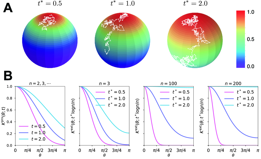
Figure 1: (A) Color maps of the exact kernel $K^{{\rm ext}}$ on $S^{2}$ at rescaled time $t^{*}=0.5,1.0,2.0$; the white paths are simulated random walks on $S^{2}$ with the Monte Carlo time approximately equal to $t=t^{*}\log 3/3$. (B) Plots of the parametrix kernel $K^{{\rm prx}}$ and exact kernel $K^{{\rm ext}}$ on $S^{n-1}$, for $n=3,100,200$, as functions of the geodesic distance.

Note that unlike $K^{{\rm prx}}(\hat{x},\hat{y};t)$, $K^{{\rm ext}}(\hat{x},\hat{y};t)$ explicitly depends on the feature dimension $n$. In general, SVM kernel hyperparameter tuning can be computationally costly for a data set with both high feature dimension and large sample size. In particular, choosing an appropriate diffusion time scale is an important challenge. On the one hand, choosing a very large value of $t$ will make the series converge rapidly; but, then, all points will become uniformly similar, and the kernel will not be very useful. On the other hand, a too small value of $t$ will make most data pairs too dissimilar, again limiting the applicability of the kernel. In practice, we thus need a guideline for a finite time scale at which the degree of “self-relatedness” is not singular, but still larger than the “relatedness” averaged over the whole hypersphere. Examining the asymptotic behavior of the exact heat kernel in high feature dimension $n$ shows that an appropriate time scale is $t\sim{\mathcal{O}}(\log n/n)$; in this regime the numerical sum in Theorem 1 satisfies a stopping condition at low orders in $\ell$ and the sample points are in moderate diffusion proximity to each other so that they can be accurately classified (Supplementary Material, Section S2.5.4).

Figure 1A illustrates the diffusion process captured by our exact kernel $K^{{\rm ext}}(\hat{x},\hat{y};t)$ in three feature dimensions at time $t=t^{*}\log 3/3$, for $t^{*}=0.5,1.0,2.0$. In Figure 1B, we systematically compared the behavior of (1) dimension-independent parametrix kernel $K^{{\rm prx}}$ at time $t=0.5,1.0,2.0$ and (2) exact kernel $K^{{\rm ext}}$ on $S^{n-1}$ at $t=t^{*}\log n/n$ for $t^{*}=0.5,1.0,2.0$ and $n=3,100,200$. By symmetry, the slope of $K^{{\rm ext}}$ vanished at the south pole $\theta=\pi$ for any time $t$ and dimension $n$. In sharp contrast, $K^{{\rm prx}}$ had a negative slope at $\theta=\pi$, again highlighting a singular behavior of the parametrix kernel. The “relatedness” measured by $K^{{\rm ext}}$ at the sweet spot $t=\log n/n$ was finite over the whole hypersphere with sufficient contrast between nearby and far away points. Moreover, the characteristic behavior of $K^{{\rm ext}}$ at $t=\log n/n$ did not change significantly for different values of the feature dimension $n$, confirming that the optimal $t$ for many classification applications will likely reside near the “sweet spot” $t=\log n/n$.

2.3 SVM classifications

Linear SVM seeks a separating hyperplane that maximizes the margin, i.e. the distance to the nearest data point. The primal formulation of SVM attempts to minimize the norm of the weight vector $\mathbf{w}$ that is normal to the separating hyperplane, subject to either hard or soft margin constraints. In the so-called Lagrange dual formulation of SVM, one applies the Representer Theorem to rewrite the weight as a linear combination of data points; in this set-up, the dot products of data points naturally appear, and kernel SVM replaces the dot product operation with a chosen kernel evaluation. The ultimate hope is that the data points will become linearly separable in the new feature space implicitly defined by the kernel.

We evaluated the performance of kernel SVM using the

1. linear kernel $K^{{\rm lin}}(\mathbf{x},\mathbf{y})=\mathbf{x}\cdot\mathbf{y}$,

2. Gaussian RBF $K^{{\rm rbf}}(\mathbf{x},\mathbf{y};\gamma)=\exp\{-\gamma|\mathbf{x}-\mathbf{y}|^{2}\}$,

3. cosine kernel $K^{{\rm cos}}(\hat{x},\hat{y})=\hat{x}\cdot\hat{y}$,

4. parametrix kernel $K^{{\rm prx}}(\hat{x},\hat{y};t)$, and

5. exact kernel $K^{{\rm ext}}(\hat{x},\hat{y};t)$,

on two independent data sets: (1) WebKB data of websites from four universities (WebKB-4-University) [21], and (2) glioblastoma multiforme (GBM) mutation data from The Cancer Genome Atlas (TCGA) with 5-fold cross-validations (CV) (Supplementary Material, Section S1). The WebKB-4-University data contained 4199 documents in total comprising four classes: student (1641), faculty (1124), course (930), and project (504); in our analysis, however, we selected an equal number of representative samples from each class, so that the training and testing sets had balanced classes. Table 1 shows the average optimal prediction accuracy scores of the five kernels for a varying number of representative samples, using 393 most frequent word features (Supplementary Material, Section S1). The exact kernel outperformed the Gaussian RBF and parametrix kernel, reducing the error by $41\%\sim 45\%$ and by $1\%\sim 7\%$, respectively. Changing the feature dimension did not affect the performance much (Table 2).

$m_{{\rm r}}$	lin	rbf	cos	prx	ext
100	74.2%	75.1%	84.4%	85.4%	85.6%
200	80.9%	82.0%	89.2%	89.6%	89.9%
300	83.2%	84.1%	89.9%	90.5%	91.1%
400	86.7%	86.1%	91.3%	91.7%	92.3%

Table 1: WebKB-4-University Document Classification. Performance test on four-class (student, faculty, course, and project) classification of WebKB-4-University word count data with different number $m_{{\rm r}}$ of representatives for each class, for $m_{{\rm r}}=100,200,300,400$. The entries show the average of optimal 5-fold cross-validation mean accuracy scores of five runs. The exact kernel (ext) reduced the error of parametrix kernel (prx) by $1\%\sim 7\%$ and the Gaussian RBF (rbf) by $41\%\sim 45\%$; the cosine kernel (cos) also reduced the error of linear kernel (lin) by $34\%\sim 43\%$.

$n$	$m_{{\rm r}}$	lin	rbf	cos	prx	ext
393	400	86.73%	86.27%	91.57%	91.99%	92.44%
726	400	86.78%	86.95%	92.62%	92.91%	93.00%
1023	400	85.56%	86.11%	92.62%	92.74%	92.91%
1312	400	85.78%	86.75%	92.56%	92.81%	93.03%

Table 2: WebKB-4-University Document Classification. Comparison of kernel SVMs on the WebKB-4-University data with a fixed sample size $m_{{\rm r}}$, but varying feature dimension $n$. To account for the randomness in selecting the representative samples using KMeans (Supplementary Material, Section S1), we performed fives runs of representative selection, and then performed CV using the training and test sets obtained from each run. Finally, we averaged the five mean CV scores to assess the performance of each classifier on the imbalanced WebKB-4-University data set. The exact (ext) and cosine (cos) kernels outperformed the Gaussian RBF (rbf) and linear (lin) kernels in various feature dimensions $n=393,726,1023,$ and $1312$, with fixed and balanced class size $m_{{\rm r}}=400$. A word was selected as a feature if its total count was greater than 1/10, 1/20, 1/30 or 1/40 times the total number of web pages in the WebKB-4-University data set, with the different thresholds corresponding to the different rows in the table. The exact kernel reduced the errors of Gaussian RBF and parametrix kernels by $45\sim 48\%$ and $1\sim 6\%$, respectively; the cosine kernel reduced the errors of linear kernel by $36\sim 49\%$.

	lin	rbf	cos	prx	ext
ZMYM4	82.9%	84.0%	83.6%	84.1%	85.1%
ADGRB3	75.7%	81.0%	78.0%	79.5%	79.3%
NFX1	73.0%	81.2%	80.9%	82.7%	82.5%
P2RX7	79.2%	84.1%	85.0%	84.0%	85.0%
COL1A2	68.4%	70.5%	72.9%	73.9%	74.2%

Table 3: TCGA-GBM Genotype Imputation. Performance test on binary classification of mutant vs. wild-type in TCGA-GBM mutation count data. The rows are different genes, the mutation statuses of which were imputed using $m_{{\rm r}}$ samples in each mutant and wild-type class. The entries show the average of optimal 5-fold cross-validation mean accuracy scores of five runs.

In the TCGA-GBM data, there were 497 samples, and we aimed to impute the mutation status of one gene – i.e., mutant or wild-type – from the mutation counts of other genes. For each imputation target, we first counted the number $m_{{\rm r}}$ of mutant samples and then selected an equal number of wild-type samples for 5-fold CV. Imputation tests were performed for top 102 imputable genes (Supplementary Material, Section S1). Table 3 shows the average prediction accuracy scores for 5 biologically interesting genes known to be important for cancer [22]:

1. ZMYM4 ($m_{{\rm r}}=33$) is implicated in an antiapoptotic activity; [23, 24];

2. ADGRB3 ($m_{{\rm r}}=37$) is a brain-specific angiogenesis inhibitor [25, 26, 27];

3. NFX1 ($m_{{\rm r}}=42$) is a repressor of hTERT transcription [28] and is thought to regulate inflammatory response [29];

4. P2RX7 ($m_{{\rm r}}=48$) encodes an ATP receptor which plays a key role in restricting tumor growth and metastases [30, 31, 32];

5. COL1A2 ($m_{{\rm r}}=61$) is overexpressed in the medulloblastoma microenvironment and is a potential therapeutic target [33, 34, 35].

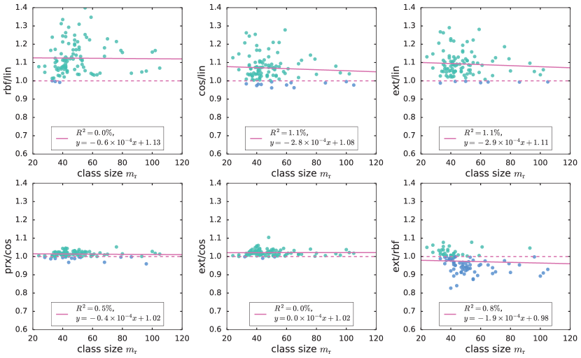
Figure 2: Comparison of the classification accuracy of SVM using linear (lin), cosine (cos), Gaussian RBF (rbf), parametrix (prx), and exact (ext) kernels on TCGA mutation count data. The plots show the ratio of accuracy scores for two different kernels. For visualization purpose, we excluded one gene with $m_{{\rm r}}=250$. The ratios rbf/lin, prx/cos, and ext/cos were essentially constant in class size $m_{{\rm r}}$ and greater than 1; in other words, the Gaussian RBF (rbf) kernel outperformed the linear (lin) kernel, while the exact (ext) and parametrix (prx) kernels outperformed the cosine (cos) kernel uniformly over all values of class size $m_{{\rm r}}$. However, the more negative slope in the linear fit of cos/lin hints that the accuracy scores of cosine and linear kernels may depend on the class size $m_{{\rm r}}$; the exact kernel also tended to outperform Gaussian RBF kernel when $m_{\rm r}$ was small.

For the remaining genes, the exact kernel generally outperformed the linear, cosine and parametrix kernels (Figure 2). However, even though the exact kernel dramatically outperformed the Gaussian RBF in the WebKB-4-University classification problem, the advantage of the exact kernel in this mutation analysis was not evident (Figure 2). It is possible that the radial degree of freedom $\sum_{i=1}^{n}x_{i}$ in this case, corresponding to the genome-wide mutation load in each sample, contained important covariate information not captured by the hyperspherical heat kernel. The difference in accuracy between the hyperspherical kernels (cos, prx, and ext) and the Euclidean kernels (lin and rbf) also hinted some weak dependence on class size $m_{\rm r}$ (Figure 2), or equivalently the sample size $m=2m_{\rm r}$. In fact, the level of accuracy showed much stronger correlation with the “effective sample size” $\tilde{m}$ related to the empirical Vapnik-Chervonenkis (VC) dimension [36, 4, 7, 37, 38] of a kernel SVM classifier (Figure 3A-E); moreover, the advantage of the exact kernel over the Guassian RBF kernel grew with the effective sample size ratio $\tilde{m}_{\rm cos}/\tilde{m}_{\rm lin}$ (Figure 3F, Supplementary Material, Section S2.5.5).

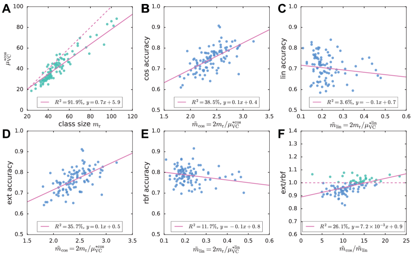
Figure 3: (A) A strong linear relation is seen between the VC-bound for cosine kernel $\mu_{{\rm VC}}^{*\cos}$ and class size $m_{{\rm r}}$. The dashed line marks $y=x$; the VC-bound for linear kernel, however, was a constant $\mu_{{\rm VC}}^{*{\rm lin}}=439$. (B-E) The scatter plots of accuracy scores for cosine (cos), linear (lin), exact (ext), and Gaussian RBF (rbf) kernels vs. the effective sample size $\tilde{m}=2m_{{\rm r}}/\mu_{{\rm VC}}^{*}$; the accuracy scores of exact and cosine kernels increased with the effective sample size, whereas those of Gaussian RBF and linear kernels tended to decrease with the effective sample size. (F) The ratio of ext vs. rbf accuracy scores is positively correlated with the ratio $\tilde{m}_{\rm cos}/\tilde{m}_{\rm lin}$ of effective sample sizes.

By construction, our definition of the hyperspherical map exploits only the positive portion of the whole hypersphere, where the parametrix and exact heat kernels seem to have similar performances. However, if we allow the data set to assume negative values, i.e. the feature space is the usual $\mathbb{R}^{n}\backslash\{0\}$ instead of $\mathbb{R}_{\geq 0}^{n}\backslash\{0\}$, then we may apply the usual projective map, where each vector in the Euclidean space is normalized by its $L^{2}$-norm. As shown in Figure 1B, the parametrix kernel is singular at $\theta=\pi$ and qualitatively deviates from the exact kernel for large values of $\theta$. Thus, when data points populate the whole hypersphere, we expect to find more significant differences in performance between the exact and parametrix kernels. For example, Table 4 shows the kernel SVM classifications of 91 S&P500 Financials stocks against 64 Information Technology stocks ($m=155$) using their log-return instances between January 5, 2015 and November 18, 2016 as features. As long as the number of features was greater than sample size, $n>m$, the exact kernel outperformed all other kernels and reduced the error of Gaussian RBF by $29\sim 51\%$ and that of parametrix kernel by $17\sim 51\%$.

$n$	$m$	lin	rbf	cos	prx	ext
475	155	98.06%	98.69%	98.69%	98.69%	99.35%
238	155	95.50%	96.77%	94.82%	96.13%	98.06%
159	155	94.86%	95.48%	95.48%	96.13%	96.79%
119	155	92.86%	93.53%	91.57%	94.15%	94.15%
95	155	91.55%	95.50%	94.19%	94.15%	94.79%

Table 4: S&P500 Stock Classification. Classifications were performed on $m=155$ stocks from S&P500 companies: 91 Financial vs. 64 Information Technology. The 475 log-return instances between January 5, 2015 and November 18, 2016 were used as features. We uniformly subsampled the instances to generate variations in the feature dimension $n$. Here, we report the mean 5-fold CV accuracy score for each kernel. Although the two classes were slightly imbalanced, all scores were much larger than the “random score” $91/155\approx 58.7\%$, calculated from the majority class size and sample size. For $n>m$, the exact (ext) kernel outperformed all other kernels and reduced the errors of Gaussian RBF (rbf) and parametrix (prx) kernels by $29\sim 51\%$ and $17\sim 51\%$, respectively. When $n<m$, the exact kernel started to lose its advantage over the Gaussian RBF kernel.

3 Discussion

This paper has constructed the exact hyperspherical heat kernel using the complete basis of high-dimensional angular momentum eigenfunctions and tested its performance in kernel SVM. We have shown that the exact kernel and cosine kernel, both of which employ the hyperspherical maps, often outperform the Gaussian RBF and linear kernels. The advantage of using hyperspherical kernels likely arises from the hyperspherical maps of feature space, and the exact kernel may further improve the decision boundary flexibility of the raw cosine kernel. To be specific, the hyperspherical maps remove the less informative radial degree of freedom in a nonlinear fashion and compactify the Euclidean feature space into a unit hypersphere where all data points may then be enclosed within a finite radius. By contrast, our numerical estimations using TCGA-GBM data show that for linear kernel SVM, the margin $M$ tends to be much smaller than the data range $R$ in order to accommodate the separation of strongly mixed data points of different class labels; as a result, the ratio $R/M$ was much larger than that for cosine kernel SVM. This insight may be summarized by the fact that the upper bound on the empirical VC-dimension of linear kernel SVM tends to be much larger than that for cosine kernel SVM, especially in high dimensions, suggesting that the cosine kernel SVM is less sensitive to noise and more generalizable to unseen data. The exact kernel is equipped with an additional tunable hyperparameter, namely the diffusion time $t$, which adjusts the curvature of nonlinear decision boundary and thus adds to the advantage of hyperspherical maps. Moreover, the hyperspherical kernels often have larger effective sample sizes than their Euclidean counterparts and, thus, may be especially useful for analyzing data with a small sample size in high feature dimensions.

The failure of the parametrix expansion of heat kernel, especially in dimensions $n\gg 3$, signals a dramatic difference between diffusion in a non-compact space and that on a compact manifold. It remains to be examined how these differences in diffusion process, random walk and topology between non-compact Euclidean spaces and compact manifolds like a hypersphere help improve clustering performance as supported by the results of this paper.

Funding

This research was supported by a Distinguished Scientist Award from Sontag Foundation and the Grainger Engineering Breakthroughs Initiative.

S1 Data preparation and SVM classification

The WebKB-4-University raw webpage data were downloaded from http://www.cs.cmu.edu/afs/cs/project/theo-20/www/data/ and processed with the python packages Beautiful Soup and Natural Language Toolkit (NLTK). Our feature extraction excluded punctuation marks and included only letters and numerals where capital letters were all converted to lower case and each individual digit 0-9 was represented by a “#.” Very infrequent words, such as misspelled words, non-English words, and words mixed with special characters, were filtered out. We selected top $393$ most frequent words as features in our classification tests; the cutoff was chosen to select frequent words whose counts across all webpage documents are greater than $10\%$ of the total number of documents. There were 4199 documents in total: student (1641), faculty (1124), course (930), and project (504).

The TCGA-GBM data were downloaded from the GDC Data Portal under the name TCGA-GBM Aggregated Somatic Mutation. The mutation count data set was extracted from the MAF file, while ignoring the detailed types of mutations and counting only the total number of mutations in each gene. Very infrequently, mutated genes were filtered out if the total number of mutations in one gene across all samples is less than $10\%$ of the total number of samples ($m=497$ samples and $n=439$ genes). We imputed the mutation status of one gene, mutant or wild-type, from the mutation counts of the remaining genes. The most imputable genes were selected using 5-fold cross-validation linear kernel SVM. Most of the mutant and wild-type samples were highly unbalanced, the ratio being typically around $1:9$; therefore, unthresholded area-under-the-curve (AUC) of the receiver operating characteristic (ROC) curve was used to quantify the classification performance of the linear kernel SVM. Mutated genes with AUC greater than $60\%$ were selected for the subsequent imputation tests.

To balance the sample size between classes, we performed K-means clustering of samples within each class, with a specified number $m_{{\rm r}}$ of centroids and took the samples closest to each centroid as representatives. For the WebKB document classifications, we used $m_{{\rm r}}\leq\min\{m_{{\rm student}},m_{{\rm faculty}},m_{{\rm course}},$ $m_{\rm project}\}$, and K-means clustering was performed in each of the four classes separately; for the TCGA-GBM data, $m_{{\rm r}}$ was chosen to be the number of samples in each mutant (minority) class, and K-means clustering was performed in the wild-type (majority) class. Since K-means might depend on the random initialization, we performed the clustering 50 times and selected the top $m_{{\rm r}}$ most frequent representatives. Five-fold stratified cross-validations (CV) were performed on the resulting balanced data sets, where training and test samples were drawn without replacement from each class. The mean CV accuracy scores across the five folds were recorded.

S2 Hyperspherical Heat Kernel

S2.1 Laplacian on a Riemannian manifold

The Laplacian on a Riemannian manifold ${\mathcal{M}}$ with metric $g_{\mu\nu}$ is the operator

$$\Delta:C^{\infty}({\mathcal{M}})\rightarrow C^{\infty}({\mathcal{M}})$$

defined as

$$\Delta\equiv\frac{1}{\sqrt{g}}\partial_{\mu}\left(\sqrt{g}g^{\mu\nu}\partial_{\nu}\right),$$ (S1)

where $g=|\det g|$, and the Einstein summation convention is used. It can be also written in terms of the covariant derivative $\nabla_{\mu}$ as

$$\Delta=g^{\mu\nu}\nabla_{\mu}\nabla_{\nu}.$$ (S2)

The covariant derivative satisfies the following properties

$$\nabla_{\mu}f=\partial_{\mu}f,\quad f\in C^{\infty}({\mathcal{M}})$$

$$\nabla_{\mu}V^{\nu}=\partial_{\mu}V^{\nu}+\Gamma_{\>\lambda\mu}^{\nu}V^{\lambda},\quad V\in T_{p}{\mathcal{M}}$$

$$\nabla_{\mu}\omega_{\nu}=\partial_{\mu}\omega_{\nu}-\Gamma_{\>\nu\mu}^{\lambda}\omega_{\lambda},\quad\omega\in T_{p}^{*}{\mathcal{M}},$$

where $\Gamma_{\>\alpha\beta}^{\lambda}$ is the Levi-Civita connection satisfying $\Gamma_{\>\alpha\beta}^{\lambda}=\Gamma_{\>\beta\alpha}^{\lambda}$ and $\nabla_{\lambda}g_{\mu\nu}=0$. To show Equation S2, recall that the Levi-Civita connection is uniquely determined by the geometry, or the metric tensor, as

$$\Gamma_{\>\alpha\beta}^{\lambda}=\frac{1}{2}g^{\lambda\rho}\left(\partial_{\alpha}g_{\beta\rho}+\partial_{\beta}g_{\alpha\rho}-\partial_{\rho}g_{\alpha\beta}\right).$$

Using the formula for determinant differentiation

$$\left[\log\left(\det\mathbf{A}\right)\right]^{\prime}={\rm tr}\left(\mathbf{A}^{\prime}\mathbf{A}^{-1}\right),$$

we can thus write

$$\Gamma_{\>\lambda\mu}^{\lambda}=\partial_{\mu}\log\sqrt{g}.$$

Hence, for any $f\in C^{\infty}({\mathcal{M}})$,

$$g^{\mu\nu}\nabla_{\mu}\nabla_{\nu}f =\nabla_{\mu}(g^{\mu\nu}\partial_{\nu}f)$$

$$=\partial_{\mu}(g^{\mu\nu}\partial_{\nu}f)+\Gamma_{\>\lambda\mu}^{\lambda}(g^{\mu\nu}\partial_{\nu}f)$$

$$=\partial_{\mu}(g^{\mu\nu}\partial_{\nu}f)+(\partial_{\mu}\log\sqrt{g})(g^{\mu\nu}\partial_{\nu}f)$$

$$=\frac{1}{\sqrt{g}}\partial_{\mu}\left(\sqrt{g}g^{\mu\nu}\partial_{\nu}\right),$$

proving the equivalence of Equation S1 and Equation S2.

S2.2 The induced metric on $S^{n-1}$

The $(n-1)$-sphere embedded in $\mathbb{R}^{n}$ can be parameterized as

$$x_{1} = \cos\theta_{1}$$

$$x_{2} = \sin\theta_{1}\cos\theta_{2}$$

$$x_{3} = \sin\theta_{1}\sin\theta_{2}\cos\theta_{3}$$

$$\vdots$$

$$x_{n-1} = \sin\theta_{1}\cdots\sin\theta_{n-2}\cos\theta_{n-1}$$

$$x_{n} = \sin\theta_{1}\cdots\sin\theta_{n-2}\sin\theta_{n-1},$$

where $0\leq\theta_{i}\leq\pi$, for $i=1,\ldots,n-2$, and $0\leq\theta_{n-1}\leq 2\pi$.

Let $\lambda:=(\partial x_{i}/\partial\theta_{j})$ denote the $n\times(n-1)$ Jacobian matrix for the above coordinate transformation. The square of the line element in $\mathbb{R}^{n}$ is given by

$$ds_{n}^{2}=\sum_{i=1}^{n}dx_{i}dx_{i}.$$

Restricted to $S^{n-1}$,

$$dx_{i}=\sum_{j=1}^{n-1}\frac{\partial x_{i}}{\partial\theta_{j}}d\theta_{j}=\sum_{j=1}^{n-1}\lambda_{ij}d\theta_{j}.$$

Therefore, on $S^{n-1}$, we have

$$ds_{n-1}^{2} =\sum_{i=1}^{n}\sum_{j,j^{\prime}=1}^{n-1}\lambda_{ij}\lambda_{ij^{\prime}}d\theta_{j}d\theta_{j^{\prime}}$$

$$=\sum_{j,j^{\prime}=1}^{n-1}\left(\sum_{i=1}^{n}\lambda_{ij}\lambda_{ij^{\prime}}\right)d\theta_{j}d\theta_{j^{\prime}}\,.$$

Hence, the induced metric on $S^{n-1}$ embedded in $\mathbb{R}^{n}$ is

$$g_{\mu\nu}=\left(\lambda^{T}\lambda\right)_{\mu\nu}.$$

After some algebraic manipulations, it can be shown that the metric is in fact diagonal and its determinant takes the form

$$g=\sin^{2(n-2)}\theta_{1}\sin^{2(n-3)}\theta_{2}\cdots\sin^{4}\theta_{n-3}\sin^{2}\theta_{n-2}.$$ (S3)

The geodesic arc length $\theta$ between $\hat{x}$ and $\hat{x}^{\prime}$ on $S^{n-1}$ is the angle given by

$$\theta\equiv\arccos\hat{x}\cdot\hat{x}^{\prime}=\arccos\sum_{i=1}^{n}\hat{x}_{i}\hat{x}_{i}^{\prime}.$$

S2.3 Laplacian in geodesic polar coordinates

In geodesic polar coordinates $(r,\xi)$ around a point, one can show using Equation S2 that the Laplacian on a $d$-dimensional Riemannian manifold ${\mathcal{M}}$ takes the form

$$\Delta=\partial_{r}^{2}+(\partial_{r}\log\sqrt{g})\partial_{r}+\Delta_{S_{r}^{d-1}},$$

where $\Delta_{S_{r}^{d-1}}$ is the Laplacian induced on the geodesic sphere $S_{r}^{d-1}$ of radius $r$. If function $f$ depends only on the geodesic distance $r$ from the fixed point, then

$$\Delta f(r)=f^{\prime\prime}(r)+\left(\log\sqrt{g}\right)^{\prime}f^{\prime}(r),$$ (S4)

where ^′ denotes the radial derivative.

For the special case when ${\mathcal{M}}$ is $S^{n-1}$, the coordinates $\theta_{1},\ldots,\theta_{n-1}$ described above correspond to the geodesic polar coordinates around the north pole, with $r=\theta_{1}$. From Equation S3, we get

$$\log\sqrt{g(x)} =(n-2)\log\sin r+(n-3)\log\sin\theta_{2}+\cdots$$

$$+\log\sin\theta_{n-2}.$$

Note that only the first terms contributes to the radial derivative.

S2.4 Euclidean heat kernel

Heat kernels in general are solutions to the heat equation

$$\left(\partial_{t}-\Delta\right)\phi=0$$

with a point-source (Dirac delta) initial condition. The heat kernel in $\mathbb{R}^{d}$ is easily found to be

$$G(\mathbf{x},\mathbf{y};t)=\left(\frac{1}{4\pi t}\right)^{\frac{d}{2}}K(\mathbf{x},\mathbf{y};t)$$ (S5)

where

$$K(\mathbf{x},\mathbf{y};t)=\exp\left(-\frac{\|\mathbf{x}-\mathbf{y}\|^{2}}{4t}\right).$$

$K$ is known as the Gaussian RBF kernel with parameter $\gamma=1/4t$. $G(\mathbf{x},\mathbf{y};t)$ is the solution to the heat equation satisfying the initial condition $G(\mathbf{x},\mathbf{y};0)=\delta(\mathbf{x}-\mathbf{y})$. Note that formally,

$$G(\mathbf{x},\mathbf{y};t)={\rm e}^{t\Delta}\delta(\mathbf{x}-\mathbf{y});$$

using the Fourier transform representation of the right-hand side then yields the expression in Equation S5.

S2.5 Exact hyperspherical heat kernel

We treat the hypersphere $S^{n-1}$ as being embedded in $\mathbb{R}^{n}$ and use the induced metric on $S^{n-1}$ to define the Laplacian. The Laplacian in $\mathbb{R}^{n}$ takes the usual form

$$\Delta=\frac{1}{r^{n-1}}\partial_{r}\left(r^{n-1}\partial_{r}\right)-\frac{\hat{L}^{2}}{r^{2}}$$ (S6)

where the differential operator $\hat{L}^{2}$ depends only on the angular coordinates. $-\hat{L}^{2}$ is the spherical Laplacian operator [18].

S2.5.1 Spherical Laplacian and its eigenfunctions

For $n=3$, the Laplacian on $\mathbb{R}^{3}$ is

$$\Delta=\frac{1}{r^{2}}\partial_{r}\left(r^{2}\partial_{r}\right)-\frac{\hat{L}^{2}}{r^{2}}$$

where $\hat{L}^{2}$ is the squared orbital angular momentum operator in quantum mechanics. Restricted to $r=1$, the Laplacian reduces to the spherical Laplacian on $S^{2}$, which is exactly the operator $-\hat{L}^{2}$ whose eigenfunctions are the spherical harmonics $Y_{lm}(\theta,\phi)$ with eigenvalue $-\ell(\ell+1)$. In this setting, $Y_{lm}(\theta,\phi)$ can be viewed as the angular component of homogeneous harmonic polynomials in $\mathbb{R}^{3}$, and this perspective will be used in the subsequent discussion of hyperspherical Laplacian. By convention, our spherical harmonics satisfy the normalization condition

$$\sum_{m=-\ell}^{\ell}|Y_{\ell m}(\theta,\phi)|^{2}=\frac{2\ell+1}{4\pi}$$

and the completeness condition

$$\sum_{\ell=0}^{\infty}\sum_{m=-\ell}^{\ell}Y_{\ell m}(\theta,\phi)Y_{\ell m}^{*}(\theta^{\prime},\phi^{\prime})=\delta(\cos\theta-\cos\theta^{\prime})\delta(\phi-\phi^{\prime}).$$

Analogous to the Euclidean case, applying the evolution operator $\exp(-\hat{L}^{2}t)$ on the initial delta distribution yields the following eigenfunction expansion of the heat kernel on $S^{2}$:

$$G(\hat{x},\hat{y};t)=\sum_{l=0}^{\infty}{\rm e}^{-\ell(\ell+1)t}\sum_{m=-\ell}^{\ell}Y_{\ell m}(\hat{x})Y_{\ell m}(\hat{y})^{*}.$$

Applying the addition theorem of spherical harmonics,

$$\frac{4\pi}{2\ell+1}\sum_{m=-\ell}^{\ell}Y_{\ell m}(\hat{x})Y_{\ell m}(\hat{y})^{*}=P_{\ell}(\hat{x}\cdot\hat{y}),$$

we finally get

$$G(\hat{x}\cdot\hat{y};t)=\sum_{\ell=0}^{\infty}\left(\frac{2\ell+1}{4\pi}\right){\rm e}^{-\ell(\ell+1)t}P_{\ell}(\hat{x}\cdot\hat{y}).$$

S2.5.2 Generalization to $S^{n-1}$

Similar to the spherical harmonics, the hyperspherical harmonics arise as the angular part of degree-$\ell$ homogeneous harmonic polynomials $h_{\ell}$ that satisfy $\Delta h_{\ell}=0$. In spherical coordinates $(r,\xi)$, we can decompose $h_{\ell}(\mathbf{x})=r^{\ell}\tilde{Y}_{\ell}(\xi)$ [17, 18], where $\tilde{Y}_{\ell}(\xi)$ is the desired hyperspherical harmonic. Using the spherical coordinate Laplacian in $\mathbb{R}^{n}$ shown in Equation S6, we get

$$0=\Delta h_{\ell}(\mathbf{x})=\tilde{Y}_{\ell}(\hat{x})\frac{1}{r^{n-1}}\partial_{r}\left(r^{n-1}\partial_{r}r^{\ell}\right)-r^{\ell-2}\hat{L}^{2}\tilde{Y}_{\ell}(\xi),$$

which can be simplified to yield the following eigenvalue equation for the hyperspherical Laplacian:

$$\hat{L}^{2}Y_{\ell\{m\}}=\ell(\ell+n-2)Y_{\ell\{m\}},$$

where the set $\{m\}$ indexes the degenerate eigenstates.

S2.5.3 Lemmas for the proof of convergence

To construct the eigenfunction expansion of the exact heat kernel and prove its convergence, we need the following lemmas [17, 18, 39]:

Lemma 1

The hyperspherical harmonics are complete on $S^{n-1}$ and resolve the $\delta$-function

$$\delta(\hat{x},\hat{y})=\sum_{\ell=0}^{\infty}\sum_{\{m\}}Y_{\ell\{m\}}(\hat{x})Y_{\ell\{m\}}^{*}(\hat{y}).$$ (S7)

Lemma 2

The hyperspherical harmonics satisfy the generalized addition theorem

$$\sum_{\{m\}}Y_{\ell\{m\}}(\hat{x})Y_{\ell\{m\}}(\hat{y})^{*}=\frac{1}{A_{S^{n-1}}}\frac{2\ell+n-2}{n-2}C_{\ell}^{\frac{n}{2}-1}(\hat{x}\cdot\hat{y}),$$

where $C_{\ell}^{\nu}(w)$ are the Gegenbauer polynomials and $A_{S^{n-1}}=2\pi^{n/2}/\Gamma\left(\frac{n}{2}\right)$ is the surface area of $S^{n-1}$.

Lemma 3

The Gegenbauer polynomials $C_{\ell}^{\alpha}(w)$ with $\alpha>0$ and $\ell\geq 0$ are bounded in the interval $w\in[-1,1]$: in particular, $C_{0}^{\alpha}(w)=1$, $C_{1}^{\alpha}(w)=\alpha w$, and thus, $|C_{1}^{\alpha}(w)|\leq\alpha$ for $w\in[-1,1]$. Finally, for $\ell\geq 2$,

$$|C_{\ell}^{\alpha}(w)|\leq\left[w^{2}c_{2\ell,2\alpha}+(1-w^{2})c_{\ell,\alpha}\right],$$

where

$$c_{\ell,\alpha}=\frac{\Gamma(\frac{\ell}{2}+\alpha)}{\Gamma(\alpha)\Gamma(\frac{\ell}{2}+1)}.$$

S2.5.4 The sweet spot of $t$

Choosing an appropriate diffusion time $t$ for the heat kernel is important for machine learning applications. Here, we use the degree of self-similarity measured by the heat kernel as a function of $t$, and propose a choice for which the self-similarity is neither too large nor too small. If $t$ is too large, then the self-similarity is roughly the uniform similarity $1/A_{S^{n-1}}$, thereby losing contrast between neighbors and outliers. By contrast, as $t$ approaches 0, the self-similarity becomes infinite, and the sense of neighborhood becomes too localized. We thus need an intermediate value of $t$, for which the self-similarity interpolates between the two limits.

The self-similarity is a special value of the heat kernel

$$G(1;t) = \sum_{\ell=0}^{\infty}{\rm e}^{-\ell(\ell+n-2)t}\frac{2\ell+n-2}{n-2}\frac{1}{A_{S^{n-1}}}C_{\ell}^{\frac{n}{2}-1}(1)$$

$$= \frac{1}{A_{S^{n-1}}}\sum_{\ell=0}^{\infty}{\rm e}^{-\ell(\ell+n-2)t}\frac{2\ell+n-2}{n-2}\frac{\Gamma(\ell+n-2)}{\Gamma(\ell+1)\Gamma(n-2)}.$$

Because the series converges rapidly for sufficiently large $t$, we can truncate the series at $\ell=\ell_{\max}$; i.e.

$$G(1;t)\approx\frac{1}{A_{S^{n-1}}}\sum_{\ell=0}^{\ell_{\max}}{\rm e}^{-\ell(\ell+n-2)t}\frac{2\ell+n-2}{n-2}\frac{\Gamma(\ell+n-2)}{\Gamma(\ell+1)\Gamma(n-2)}.$$

In the large $n$ limit, we can bound the sum as

$$G(1;t)\leq\frac{1}{A_{S^{n-1}}}\sum_{\ell=0}^{\ell_{\max}}\left({\rm e}^{-nt}\right)^{\ell}\frac{n^{\ell}}{\ell!}\leq\frac{\exp\left(n{\rm e}^{-nt}\right)}{A_{S^{n-1}}}.$$

To keep the self-similarity finite, but larger than the uniform similarity, suggests the choice for $t$ of order $\log n/n$, at which the self-similarity is roughly ${\rm e}/A_{S^{n-1}}$. We thus search for an optimal value of $t$ around $\log n/n$.

S2.5.5 SVM Classification

In the main text, we denoted the parametrix and exact heat kernels normalized by self-similarity as the “parametrix kernel” and “exact kernel,” respectively. We then used the linear (lin), Gaussian RBF (rbf), cosine (cos), parametrix (prx), and exact (ext) kernels in SVM to (1) classify WebKB-4-University web pages into four classes: student, faculty, course, and project; and (2) impute the binary mutation status of genes in TCGA-GBM data. The kernel SVM classification results shown in the main text indicated that the cosine kernel usually outperformed the linear kernel, most likely as a pure consequence of the hyperspherical geometry, as we argue below. The exact kernel outperformed the Gaussian RBF kernel for the WebKB document data, but the advantage of exact kernel diminished in the TCGA mutation count data. Figure 2 compares the accuracy of SVM using different kernels on the TCGA-GBM data, where the accuracy ratios rbf/lin, cos/lin, ext/lin, prx/cos, and ext/cos were greater than 1 for most class sizes $m_{{\rm r}}$. Interestingly, the ratio cos/lin showed some dependence on the sample size $m_{{\rm r}}$, and the exact kernel also tended to outperform the Gaussian RBF kernel when $m_{{\rm r}}$ was small; in general, we noted that the hyperspherical kernels tended to outperform the Euclidean kernels in small-sample-size classification problems. This pattern may be understood by examining the generalization error of kernel SVM as follows.

Intuitively, if a generic classifier were closely acquainted with the population distribution of data through a large sample size, then its predictions would be more generalizable to unseen samples. The “largeness” of sample size $m$, however, is not explicitly quantifiable unless we have a natural unit for it. Statistical learning theory [36, 37, 7] provides such a unit associated with a probabilistic upper bound on generalization errors. That is, with probability at least $1-\eta$, the generalization error of a binary SVM classification is bounded from above by

$$F(\tilde{m};\mu_{{\rm VC}},\eta)=\sqrt{\frac{1}{\tilde{m}}\left[\left(\log 2\tilde{m}+1\right)-\frac{\log\frac{\eta}{4}}{\mu_{{\rm VC}}}\right]}$$

where $\mu_{{\rm VC}}$ is the VC-dimension of the classifier, and $\tilde{m}=m/\mu_{{\rm VC}}$ is the effective sample size. The derivative of $F(\tilde{m};\mu_{{\rm VC}},\eta)$ with respect to $\tilde{m}$ is proportional to a positive factor times $-\log\left[(2\tilde{m})^{\mu_{{\rm VC}}}4/\eta\right]$. Thus, the upper bound decreases with $\tilde{m}$ when $(2\tilde{m})^{\mu_{{\rm VC}}}>\eta/4$, and increases otherwise; the critical effective sample size $\tilde{m}_{{\rm crt}}=\frac{1}{2}\cdot(\eta/4)^{1/\mu_{{\rm VC}}}\approx\frac{1}{2}$ for typical values of $\mu_{{\rm VC}}>100$ and $\eta\in[10^{-3},0.1]$. The VC dimension of a linear kernel SVM can be estimated using an empirical upper bound [37, 38]

$$\mu_{VC}\leq\mu_{VC}^{*}=\min\left\{n,\frac{R^{2}}{M^{2}}\right\}+1,$$

where $n$ is the feature space dimension, $R$ is the radius of the smallest ball in feature space that encloses all data points, and $M$ is the SVM margin. We evaluated the bound $\mu_{{\rm VC}}^{*}$ for the TCGA-GBM mutation count data with $C=1$, and found that the linear kernel had $R^{2}/M^{2}\approx 6\times 10^{3}$ and thus that $\mu_{{\rm VC}}^{*{\rm lin}}=n+1\approx 4\times 10^{2}$. By contrast, the cosine kernel, which is a linear kernel in the hyperspherically transformed space with $R\leq 1$, had $\mu_{{\rm VC}}^{*{\rm cos}}$ approximately in the range $20\sim 100\ll\mu_{{\rm VC}}^{*{\rm lin}}$, as shown in Figure 3A. This reduction in the VC-dimension is likely responsible for the classification improvement of the cosine kernel over the linear kernel. We thus found that $\tilde{m}_{\cos}=2m_{{\rm r}}/\mu_{{\rm VC}}^{*\cos}>\tilde{m}_{\rm crt}$, while $\tilde{m}_{{\rm lin}}=2m_{{\rm r}}/\mu_{{\rm VC}}^{*{\rm lin}}<\tilde{m}_{\rm crt}$ for the TCGA-GBM data, and that the cosine kernel accuracy increased with effective sample size, whereas the linear kernel accuracy tended to decrease (Figure 3B,C, consistent with the analysis of the upper bound on generalization error $F(\tilde{m};\mu_{{\rm VC}},\eta)$. In addition, the Gaussian RBF and exact kernels followed similar trends as the linear and cosine kernels, respectively (Figure 3D,E). Similar to the cosine kernel, the exact kernel likely inherited the reduction in VC-dimension from the hyperspherical map; as a result, the accuracy of the exact kernel also increased with $\tilde{m}_{\cos}$, but with slightly higher accuracy due to the additional tunable parameter $t$ that can adjust the curvature of nonlinear decision boundaries. Moreover, the cases of small sample size where the exact kernel outperformed the Gaussian RBF kernel corresponded to the cases of larger effective sample size ratio $\tilde{m}_{\rm cos}/\tilde{m}_{\rm lin}$ (Figure 3F).

References

- [1] Lafferty J, Lebanon G. Diffusion Kernels on Statistical Manifolds. Journal of Machine Learning Research 6 (2005) 129–163.
- [2] Hastie T, Tibshirani R, Friedman J. The Elements of Statistical Learning. Data Mining, Inference, and Prediction (Springer Science & Business Media) (2013). doi:10.1111/j.1467-985X.2010.00646˙6.x.
- [3] Evgeniou T, Pontil M. Support Vector Machines: Theory and Applications. Machine Learning and Its Applications (Berlin, Heidelberg: Springer Berlin Heidelberg) (2001), 249–257. doi:10.1007/3-540-44673-7˙12.
- [4] Boser BE, Guyon IM, Vapnik VN. A training algorithm for optimal margin classifiers (New York, New York, USA: ACM) (1992). doi:10.1145/130385.130401.
- [5] Cortes C, Vapnik V. Support-Vector Networks. Machine learning 20 (1995) 273–297. doi:10.1023/A:1022627411411.
- [6] Freund Y, Schapire RE. Large Margin Classification Using the Perceptron Algorithm. Machine learning 37 (1999) 277–296. doi:10.1023/A:1007662407062.
- [7] Guyon I, Boser B, Vapnik V. Automatic Capacity Tuning of Very Large VC-dimension Classifiers. Advances in Neural Information Processing Systems (1993) 147–155.
- [8] Kaufman L, Rousseeuw PJ. Finding Groups in Data. An Introduction to Cluster Analysis (Hoboken, NJ, USA: John Wiley & Sons) (2009). doi:10.1002/9780470316801.
- [9] Belkin M, Niyogi P, Sindhwani V. Manifold Regularization: A Geometric Framework for Learning from Labeled and Unlabeled Examples. Journal of Machine Learning Research 7 (2006) 2399–2434.
- [10] Aronszajn N. Theory of reproducing kernels. Transactions of the American mathematical society 68 (1950) 337. doi:10.2307/1990404.
- [11] Paulsen VI, Raghupathi M. An Introduction to the Theory of Reproducing Kernel Hilbert Spaces (Cambridge Studies in Advanced Mathematics) (Cambridge University Press) (2016).
- [12] Berger M, Gauduchon P, Mazet E. Le spectre d’une variete riemannienne (Springer) (1971).
- [13] Hsu EP. Stochastic analysis on manifolds, volume 38 of Graduate Studies in Mathematics (American Mathematical Society) (2002).
- [14] Varopoulos NT. Random walks and Brownian motion on manifolds (Symposia Mathematica) (1987).
- [15] Ng A, Jordan M, Weiss Y, Dietterich T, Becker S. Advances in Neural Information Processing Systems, 14, chapter On spectral clustering: analysis and an algorithm (2002).
- [16] Coifman RR, Lafon S. Diffusion maps. Applied and Computational Harmonic Analysis 21 (2006) 5–30. doi:10.1016/j.acha.2006.04.006.
- [17] Atkinson K, Han W. Spherical Harmonics and Approximations on the Unit Sphere: An Introduction (Springer Science & Business Media) (2012).
- [18] Wen ZY, Avery J. Some properties of hyperspherical harmonics. Journal of Mathematical Physics 26 (1985) 396–9. doi:10.1063/1.526621.
- [19] Stone M, Goldbart P. Mathematics for physics: a guided tour for graduate students. Cambridge University Press, Cambridge (2009). doi:10.1017/CBO9780511627040.
- [20] Grigor’yan A. Analytic and geometric background of recurrence and non-explosion of the Brownian motion on Riemannian manifolds. Bulletin of the American Mathematical Society 36 (1999) 135–249. doi:10.1090/S0273-0979-99-00776-4.
- [21] Craven M, McCallum A, PiPasquo D, Mitchell T. Learning to extract symbolic knowledge from the World Wide Web. Proceedings of the National Conference on Artificial Intelligence (1998) 509–516.
- [22] Hanahan D, Weinberg RA. Hallmarks of Cancer: The Next Generation. Cell 144 (2011) 646–674. doi:10.1016/j.cell.2011.02.013.
- [23] Smedley Dea. SHORT COMMUNICATION Cloning and Mapping of Members of the MYM Family (1999) 1–4.
- [24] Shchors K, Yehiely F, Kular RK, Kotlo KU, Brewer G, Deiss LP. Cell death inhibiting RNA (CDIR) derived from a 3’-untranslated region binds AUF1 and heat shock protein 27. Journal of Biological Chemistry 277 (2002) 47061–47072. doi:10.1074/jbc.M202272200.
- [25] Zohrabian VM, Nandu H, Gulati N. Gene expression profiling of metastatic brain cancer. Oncology Reports (2007).
- [26] Kaur B, Brat DJ, Calkins CC, Van Meir EG. Brain Angiogenesis Inhibitor 1 Is Differentially Expressed in Normal Brain and Glioblastoma Independently of p53 Expression. The American Journal of Pathology 162 (2010) 19–27. doi:10.1016/S0002-9440(10)63794-7.
- [27] Hamann J, Aust G, Araç D, Engel FB, Formstone C, Fredriksson R, et al. International Union of Basic and Clinical Pharmacology. XCIV. Adhesion G protein-coupled receptors. Pharmacological Reviews 67 (2015) 338–367. doi:10.1124/pr.114.009647.
- [28] Yamashita S, Fujii K, Zhao C, Takagi H, Katakura Y. Involvement of the NFX1-repressor complex in PKC--induced repression of hTERT transcription. Journal of Biochemistry (2016) mvw038–5. doi:10.1093/jb/mvw038.
- [29] Song Z, Krishna S, Thanos D, Strominger JL, Ono SJ. A novel cysteine-rich sequence-specific DNA-binding protein interacts with the conserved X-box motif of the human major histocompatibility complex class II genes via a repeated Cys-His domain and functions as a transcriptional repressor. Journal of Experimental Medicine 180 (1994) 1763–1774. doi:10.1084/jem.180.5.1763.
- [30] Adinolfi E, Capece M, Franceschini A, Falzoni S. Accelerated tumor progression in mice lacking the ATP receptor P2X7. Cancer research 75 (2015) 635–644. doi:10.1158/0008-5472.CAN-14-1259.
- [31] Gómez-Villafuertes R, García-Huerta P, Díaz-Hernández JI, Miras-Portugal MT. PI3K/Akt signaling pathway triggers P2X7 receptor expression as a pro-survival factor of neuroblastoma cells under limiting growth conditions. Nature Publishing Group 5 (2015) 1–15. doi:10.1038/srep18417.
- [32] Liñán-Rico A, Turco F, Ochoa-Cortes F, Harzman A, Needleman BJ, Arsenescu R, et al. Molecular Signaling and Dysfunction of the Human Reactive Enteric Glial Cell Phenotype. Inflammatory Bowel Diseases 22 (2016) 1812–1834. doi:10.1097/MIB.0000000000000854.
- [33] Anderton JA, Lindsey JC. Global analysis of the medulloblastoma epigenome identifies disease-subgroup-specific inactivation of COL1A2. Neuro-Oncology (2008). doi:10.1215/15228517-2008-048).
- [34] Liang Y, Diehn M, Bollen AW, Israel MA, Gupta N. Type I collagen is overexpressed in medulloblastoma as a component of tumor microenvironment. Journal of Neuro-Oncology 86 (2007) 133–141. doi:10.1007/s11060-007-9457-5.
- [35] Schwalbe EC, Lindsey JC, Straughton D, Hogg TL, Cole M, Megahed H, et al. Rapid diagnosis of medulloblastoma molecular subgroups. Clinical Cancer Research 17 (2011) 1883–1894. doi:10.1158/1078-0432.CCR-10-2210.
- [36] Vapnik VN. The Nature of Statistical Learning Theory (Springer Science & Business Media) (2013).
- [37] Vapnik V, Levin E, Le Cun Y. Measuring the VC-dimension of a learning machine. Neural Computation 6 (1994) 851–876. doi:10.1162/neco.1994.6.5.851.
- [38] Paliouras G, Karkaletsis V, Spyropoulos CD. Machine Learning and Its Applications. Advanced Lectures (Springer) (2003).
- [39] Lorch L. Inequalities for ultraspherical polynomials and the gamma function. Journal of Approximation Theory 40 (1984) 115–120. doi:10.1016/0021-9045(84)90020-0.