Solving Moment Hierarchies for Chemical Reaction Networks

Abstract

The study of Chemical Reaction Networks (CRN’s) is a very active field. Earlier well-known results Feinberg (1987); Anderson et al. (2010) identify a topological quantity called deficiency, for any CRN, which, when exactly equal to zero, leads to a unique factorized steady-state for these networks. No results exist however for the steady states of non-zero-deficiency networks. In this paper, we show how to write the full moment-hierarchy for any non-zero-deficiency CRN obeying mass-action kinetics, in terms of equations for the factorial moments. Using these, we can recursively predict values for lower moments from higher moments, reversing the procedure usually used to solve moment hierarchies. We show, for non-trivial examples, that in this manner we can predict any moment of interest, for CRN’s with non-zero deficiency and non-factorizable steady states.

I Introduction

Models of Chemical Reaction Networks (CRN’s) are ubiquitious in the study of biochemistry, systems biology, ecology and epidemiology. They provide a framework within which even several models studied in physics, may be cast. CRN’s are defined by a set of species, complexes and reactions which, when taken together, specify the system of interest (see Figs. 1 and 2). The mathematical modeling of CRN’s is usually carried out either through the study of deterministic ODE’s (or rate equations) which specify the mean behaviour of the concentrations of the different species, or by modeling the stochastic variability of species counts as a continuous-time Markov chain, where a transition occurs every time a reaction takes place. One of the major results pertaining to deterministic models of CRN’s is the deficiency zero theorem Feinberg (1987); Horn and Jackson (1972); Feinberg (1979). This relates a topological quantity called the deficiency (a non-negative integer index, denoted by $\delta$) to the existence, uniqueness, and stability of positive fixed points of the rate equations. In particular, when $\delta=0$ for CRN’s which are weakly reversible , there is a unique, asymptotically stable equilibrium, for any choice of (positive) rate constants. A few theorems exist for deterministically-modeled CRN’s with $\delta>0$ as well Feinberg (1987); Craciun and Feinberg (2005); Haixia (2011), which either affirm that a given network is capable of multistationarity or can rule out this possibility (See Joshi and Shiu (2015) for a recent survey).

Modeling CRN’s by ODE’s is however expected to be accurate only when species concentrations are high. When this is not the case, such as in, for example, gene expression Elowitz et al. (2002); Ozbudak et al. (2002), cell signaling Lestas et al. (2010) or enzymatic processes Xie (2001), then a stochastic modeling of CRN’s is more appropriate. A major result for this class of models is the theorem by Anderson, Craciun and Kurtz (ACK) Anderson et al. (2010) (motivated by earlier work on queueing theory by Kelly Kelly (1979)), who show that if the conditions of the deficiency zero theorem hold for a deterministically modeled CRN, then the corresponding stochastic system has a product-form steady state. There has also been work done Anderson et al. (2014) on the extinction time for certain reactions in stochastic models of CRN’s of deficiency one. However, no general results exist for obtaining the steady-state behaviour of CRN’s with $\delta>0$.

This absence of general results reflects a deeper and more fundamental feature of CRN’s: unlike simple random walks on ordinary graphs for which abundant results exist, the elementary reaction events in CRN’s involve concurrency in the conversion of inputs to outputs  Danos et al. (2008); Harmer et al. (2010). The underlying topology of a CRN is a multihypergraph rather than an ordinary graph Andersen et al. (2013, 2014); fewer results exist for hypergraphs because generic problems of search or optimization are computationally hard Berge (1973); Andersen et al. (2012). The reflection of these difficulties in CRN moment hierarchies is that moment equations at any order couple to moments at higher order, leading to an infinite hierarchy of equations. The standard way to deal with these is via moment-closure schemes Schnoerr et al. (2015), which however are ad-hoc and sometimes give unphysical results Schnoerr et al. (2017). In this paper, we take a different point of view. We show, for a generic mass-action CRN with arbitrary value of $\delta$, that the equations for the factorial moments (FM), provide a better starting point for solving the infinite moment-hierarchy. The structure of these equations facilitates recursively writing FM ratios at lower-order in terms of FM ratios at higher order. The recursions can then be solved, exactly in some cases, to obtain any moment of interest. Our results are also applicable to any non-equilibrium process describable as a mass-action CRN, such as for example, the zero-range process Evans and Hanney (2005) .

II Framework and Results

In what follows, we develop a convenient formalism for describing CRN’s, by combining a network decomposition made standard by CRN-theory Feinberg (1979); Gunawardena (2003) with the well-known stochastic process formalism due to Doi Doi (1976). To our knowledge, no one has combined these two methods earlier. The description of CRN’s simplifies considerably within this framework. In addition this formalism is crucial to understanding why the equations for the FM have the structure they do. We hence utilize two simple examples of CRN’s with non-zero deficiency, to explain both the formalism and our results. We also provide a definition for the very important concept of deficiency.

II.1 Two examples

Our first example is the following minimal model with just one species and $\delta=1$,

Figure 1: A compact graphical representation for a CRN: The red filled circle with label ${\rm A}$ represents the species ${\rm A}$ while each open circle represents a complex, such as $2{\rm A}$. The number of solid lines connecting each species to each complex, represents the stoichiometry of the complex. Each dashed line connecting two complexes represents a reaction.

Its reaction scheme is

$${\rm A} \xrightleftharpoons[\epsilon]{\alpha}2{\rm A}\xrightleftharpoons[\beta]{\epsilon}3{\rm A}$$ (1)

Another example is the following CRN with two species and $\delta=2$:

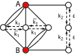
Figure 2: A CRN involving two species ${\rm A}$ and ${\rm B}$. The complex with no solid lines attached to it is the null node $\varnothing$.

Its reaction scheme is

$${\rm B}\xrightleftharpoons[\epsilon]{k_{2}}\varnothing\xrightleftharpoons[k_{2}]{\epsilon}{\rm A}$$

$$2{\rm B}+{\rm A}\xrightleftharpoons[k_{1}]{{\bar{k}}_{1}}{\rm A}+{\rm B}\xrightleftharpoons[{\bar{k}}_{1}]{k_{1}}2{\rm A}+{\rm B}$$ (2)

In the description of CRN’s two matrices conventionally appear Feinberg (1979); Gunawardena (2003). An Adjacency matrix, denoted by ${\cal{A}}$, is the matrix of transition rates among complexes. The matrix element ${\cal{A}}_{ij}$ for $i\neq j$ denotes the transition (if any) that takes complex $j$ to complex $i$, with ${\cal{A}}_{jj}\equiv-\sum_{i}{\cal{A}}_{ij}$. $\cal{A}$ has, by definition, a zero left eigenvector $\left[1,1,..1\right]$.

For the network in Fig. 1 the adjacency matrix is

$$\cal{A}=\left[\begin{array}[]{rrr}-\alpha&\epsilon&0\\ \alpha&-2\epsilon&\beta\\ 0&\epsilon&-\beta\\ \end{array}\right].$$ (3)

For the network in Fig. 2, $\cal{A}$ is a $6\times 6$ matrix over the $6$ complexes: $\varnothing$, $\rm A$, $\rm B$, $\rm{A+B}$, $\rm{2A+B}$ and $\rm{A+2B}$.

$$\cal{A}=\left[\begin{array}[]{rrrrrr}-2\epsilon&k_{2}&k_{2}&0&0&0\\ \epsilon&-k_{2}&0&0&0&0\\ \epsilon&0&-k_{2}&0&0&0\\ 0&0&0&-2k_{1}&{\bar{k}}_{1}&{\bar{k}}_{1}\\ 0&0&0&k_{1}&-{\bar{k}}_{1}&0\\ 0&0&0&k_{1}&0&-{\bar{k}}_{1}\\ \end{array}\right].$$ (4)

We assume mass-action rates (as in earlier work Feinberg (1987); Anderson et al. (2010)): if ${\rm n}_{a}$ is the number of particles of species ${\rm A}$, the rate at which complex ${\rm A}$ is converted to any other complex is the rate constant times ${\rm n}_{a}$. Similarly the rate at which complex $2{\rm A}$ takes part in any reaction is ${\rm n}_{a}\left({\rm n}_{a}-1\right)$, etc.

The other matrix which is useful to define is the stoichiometric matrix $Y$. An element $y_{p,i}$ of this matrix is the amount of species $p$ in complex $i$. We denote by $Y_{p}$, the $p^{th}$ row of this matrix.

For example, in the reaction scheme of Eq. (1), $Y$ is a row vector given by

$$Y=\left[\begin{array}[]{ccc}1&2&3\end{array}\right]$$ (5)

For the reaction scheme of Eq. (2), the $Y$ matrix is

$$Y=\left[\begin{array}[]{cccccc}0&1&0&1&2&1\\ 0&0&1&1&1&2\\ \end{array}\right]$$ (6)

where the first row $Y_{1}$ refers to species $\rm A$, the second row $Y_{2}$ to species $\rm B$ and the columns $i$ refer to the complexes in the order mentioned above.

The time-evolution of the species in a CRN, is described by a master equation for the probability ${\rho}_{{\rm n}}$, where ${\rm n}\equiv\left[{\rm n}_{p}\right]$ is a column vector, with components which are the instantaneous numbers of the different species $p$.

For example, for the CRN of Eq. (1), the master equation is

$${\dot{\rho}}_{\rm n} =\left\{\left(e^{-\partial/\partial{\rm n}}-1\right)\left[\alpha{\rm n}+\epsilon{\rm n}\left({\rm n}-1\right)\right]\right.$$

$$\phantom{=}\mbox{}+\left.\left(e^{\partial/\partial{\rm n}}-1\right)\left[\epsilon{\rm n}\left({\rm n}-1\right)+\beta{\rm n}\left({\rm n}-1\right)\left({\rm n}-2\right)\right]\right\}{\rho}_{\rm n}.$$ (7)

where the operators $e^{-\partial/\partial{\rm n}}$ (or $e^{\partial/\partial{\rm n}}$) act on any function $f\!\left({\rm n}\right)$ and convert it to $f\!\left({\rm n}-1\right)$ ($f\!\left({\rm n}+1\right)$ respectively) Smith (2011).

For the network of Fig. 2, $\rm n$ becomes a two-component index to $\rho$, which evolves under

$${\dot{\rho}}_{\rm n} =\left\{\left(e^{-\partial/\partial{\rm n}_{a}}-1\right)\left[\epsilon+k_{1}{\rm n}_{b}{\rm n}_{a}\right]\right.$$

$$\phantom{=}\mbox{}+\left.\left(e^{\partial/\partial{\rm n}_{a}}-1\right)\left[k_{2}{\rm n}_{a}+{\bar{k}}_{1}{\rm n}_{b}{\rm n}_{a}\left({\rm n}_{a}-1\right)\right]\right.$$

$$\phantom{=}\mbox{}+\left.\left(e^{-\partial/\partial{\rm n}_{b}}-1\right)\left[\epsilon+k_{1}{\rm n}_{a}{\rm n}_{b}\right]\right.$$

$$\phantom{=}\mbox{}+\left.\left(e^{\partial/\partial{\rm n}_{b}}-1\right)\left[k_{2}{\rm n}_{b}+{\bar{k}}_{1}{\rm n}_{a}{\rm n}_{b}\left({\rm n}_{b}-1\right)\right]\right\}{\rho}_{\rm n}$$ (8)

In general, for a CRN with $P$ species, the master equation is more conveniently written in terms of an equation for the generating function $\phi(z)\equiv\sum_{{\rm n}}\left(\prod_{p=1}^{P}z_{p}^{{{\rm n}}_{p}}\right){\rho}_{{\rm n}}$ where $z\equiv\left[z_{p}\right]$ is a vector. The generating function evolves under a Liouville equation of the form

$$\frac{\partial\phi}{\partial\tau}=-\mathcal{L}\phi$$

$$\mbox{shorthand for }\quad\frac{\partial}{\partial\tau}\phi\!\left(z\right) =-\mathcal{L}\!\left(z,\frac{\partial}{\partial z}\right)\phi\!\left(z\right).$$ (9)

$\mathcal{L}$ is called the Liouville Operator.

II.2 The Liouvillian

$\mathcal{L}$ has a well-known representation, due to Doi Doi (1976), in terms of raising and lowering operators $a^{\dagger}$ and $a$. We provide a brief introduction to the Doi algebra below . The Doi algebra uses the following correspondence:

$$z_{p} \rightarrow a^{\dagger}_{p} \frac{\partial}{\partial z_{p}} \rightarrow a_{p}.$$ (10)

It follows that the operators obey the conventional commutation algebra

$$\left[a_{p},a^{\dagger}_{q}\right]={\delta}_{pq},$$ (11)

where ${\delta}_{pq}$ is the Kronecker $\delta$.

Defining formal right-hand and left-hand null states,

$$1 \rightarrow\left|0\right) \int d^{P}\!z\,{\delta}^{P}\!\left(z\right) \rightarrow\left(0\right|$$ (12)

(where ${\delta}^{P}\!\left(z\right)$ is the Dirac $\delta$ in $P$ dimensions, and the inner product of the null states is normalized: $\left(0\mid 0\right)=1$), for any vector ${\rm n}\equiv\left[{\rm n}_{p}\right]$,

$$\prod_{p=1}^{P}{a_{p}^{\dagger}}^{{{\rm n}}_{p}}\left|0\right)\equiv\left|{\rm n}\right).$$ (13)

With these steps, the generating function $\phi$ becomes

$$\phi\!\left(z\right)=\sum_{{\rm n}}\prod_{p=1}^{P}z_{p}^{{{\rm n}}_{p}}{\rho}_{{\rm n}} \rightarrow\sum_{{\rm n}}{\rho}_{{\rm n}}\left|{\rm n}\right)\equiv\left|\phi\right).$$ (14)

The Liouville equation in this language takes the form

$$\frac{\partial\left|\phi\right)}{\partial\tau}=-\mathcal{L}\!\left(a_{p},a_{p}^{\dagger}\right)\left|\phi\right).$$ (15)

For example, the Liouville operator $\mathcal{L}$ for the network of Fig. 1 (and Eq. 1) is

$$\mathcal{L} =\left(1-a^{\dagger}\right)\left[\alpha a^{\dagger}a-\epsilon\left(1-a^{\dagger}\right)a^{\dagger}a^{2}-\beta{a^{\dagger}}^{2}a^{3}\right]$$

$$=\left(1-a^{\dagger}\right)\left(a^{\dagger}\!a\right)\left[\left(\alpha-\epsilon a\right)+\left(a^{\dagger}\!a-1\right)\left(\epsilon-\beta a\right)\right].$$ (16)

The Liouville operator corresponding to the two-species network (Fig. 2) is

$$\mathcal{L} =\left(1-a^{\dagger}\right)\left[\left(\epsilon-k_{2}a\right)+\left(b^{\dagger}\!b\right)\left(a^{\dagger}\!a\right)\left(k_{1}-{\bar{k}}_{1}a\right)\right]$$

$$\phantom{=}\mbox{}+\left(1-b^{\dagger}\right)\left[\left(\epsilon-k_{2}b\right)+\left(a^{\dagger}\!a\right)\left(b^{\dagger}\!b\right)\left(k_{1}-{\bar{k}}_{1}b\right)\right].$$ (17)

where $\left(a^{\dagger},a\right)$ and $\left(b^{\dagger},b\right)$, are creation and annihilation operators for the number components ${\rm n}_{a}$ and ${\rm n}_{b}$, respectively.

The Liouvillian may be written more compactly in terms of the matrices $\cal{A}$ and $Y$. To accomplish this, we need to introduce a little more notation. Define a column vector,

$${\psi}_{Y}^{i}\!\left(a\right) \equiv\prod_{p}\left(a_{p}\right)^{y_{p,i}}$$ (18)

${\psi}_{Y}^{\dagger}\equiv{\left[{{\psi}^{\dagger}}_{Y}^{i}\right]}^{T}$ is then a row vector of components defined on the indices $i$ ,

$${{\psi}^{\dagger}}_{Y}^{i}\!\left(a^{\dagger}\right)\equiv\prod_{p}\left({a^{\dagger}}_{p}\right)^{y_{p,i}}$$ (19)

For example, for the two-species network, these are simply

$${\psi}^{\dagger} =\left[\begin{array}[]{cccccc}1&a^{\dagger}&b^{\dagger}&a^{\dagger}b^{\dagger}&{a^{\dagger}}^{2}b^{\dagger}&a^{\dagger}{b^{\dagger}}^{2}\end{array}\right]$$ (21)

$${\left(\psi\right)}^{T} =\left[\begin{array}[]{cccccc}1&a&b&ab&a^{2}b&ab^{2}\end{array}\right]$$ (23)

In this formalism, the Liouville operator takes on the simple form,

$$-\mathcal{L} ={\psi}^{\dagger}_{Y}{\cal A}{\psi}_{Y}$$ (24)

II.3 The Moment Hierarchy

Entirely equivalent to solving the master equation or the Liouville equation, is to solve the moment hierarchy, namely to compute the time-dependent values of all the relevant moments in the problem. The set of equations for all these moments, obtained directly from the master equation or the Liouville equation, is referred to as the moment hierarchy, because usually lower-order moments couple to higher-order ones, resulting in an infinite hierarchy of equations. Solving the moment hierarchy is hence by no means a simple task and often involves making approximations. In what follows, we demonstrate that for any mass-action CRN, the equations for the factorial moments (rather than the equations for ordinary moments) take on a particularly tractable form. For the examples we consider, we show how this tractability helps in solving the entire moment hierarchy in the steady state.

In order to see this, we first need to write down the equations for the moments. The time dependence of arbitrary moments is easily extracted from the Liouville equation via the Glauber inner product, which is a standard construction Cardy (1999); Mattis and Glasser (1998). In the interest of completeness, we provide all relevant details in what follows. As mentioned earlier, we will prefer instead to look at the factorial moments (FM). In order to define these, consider, for a single component ${{\rm n}}_{p}$ and power $k_{p}$, the quantity

$${{\rm n}}_{p}^{\underline{k_{p}}} \equiv\frac{{{\rm n}}_{p}!}{\left({{\rm n}}_{p}-k_{p}\right)!} ;\;k_{p}\leq{{\rm n}}_{p}$$

$$\equiv 0 ;\;k_{p}>{{\rm n}}_{p}.$$ (25)

For a vector $k\equiv\left[k_{p}\right]$ of powers and a vector ${\rm n}$ of instanstaneous numbers of the species, we introduce the factorial moment indexed by $k$, as the expectation

$$\left<{\rm n}^{\underline{k}}\right>\equiv\left<\prod_{p}{{\rm n}}_{p}^{\underline{k_{p}}}\right>.$$ (26)

The FM are generated by the action of the lowering operator on the number state. In particular, for any non-negative integer $k_{p}$,

$$a_{p}^{k_{p}}\left|{\rm n}\right) ={{\rm n}}_{p}^{\underline{k_{p}}}\left|{\rm n}-k_{p}\right)$$

$${a^{\dagger}_{p}}^{k_{p}}a_{p}^{k_{p}}\left|{\rm n}\right) ={{\rm n}}_{p}^{\underline{k}}\left|{\rm n}\right).$$ (27)

where $\left|{\rm n}-k_{p}\right)$ is the number state with $k_{p}$ subtracted from ${{\rm n}}_{p}$ and all ${{\rm n}}_{q}$ for $q\neq p$ unchanged.

The time dependence of the FM is then simply given by

$$\frac{\partial}{\partial\tau}\left<\prod_{p}{{\rm n}}_{p}^{\underline{k_{p}}}\right>\equiv\frac{\partial}{\partial\tau}\left<{\rm n}^{\underline{k}}\right> =\left(0\right|e^{\sum_{q}a_{q}}{\prod_{p}\left(a_{p}\right)}^{k_{p}}\left(-\mathcal{L}\right)\left|\phi\right)$$

$$=\left(0\right|e^{\sum_{q}a_{q}}{\prod_{p}\left(a_{p}\right)}^{k_{p}}{\psi}^{\dagger}_{Y}\!\left(a^{\dagger}\right){\cal A}\,{\psi}_{Y}\!\left(a\right)\left|\phi\right)$$ (28)

In writing Eq. (28), the fact that all number states are normalized with respect to the Glauber inner product, defined by

$$\left(0\right|e^{\sum_{p}a_{p}}\left|{\rm n}\right)=1,\quad\forall{\rm n}$$ (29)

is used.

The Glauber inner product with a generating function is simply the trace of the underlying probability density:

$$\left(0\right|e^{\sum_{p}a_{p}}\left|\phi\right)=\sum_{{\rm n}}{\rho}_{{\rm n}}=1.$$ (30)

Eq. (28) denotes the time-evolution of a generic FM for a CRN with an arbitrary number of species. In particular, the equation for the first moment takes on a simple form. Note that a first moment, for a CRN of $P$ species, is specified by a vector $k\equiv\left[k_{p}\right]$, with only one of the $k_{p}$’s being non-zero (and having the value $1$). This corresponds to computing the average value of the number of one specific species $p$. In this case, from Eq. (28), we need only to commute $a_{p}$ through ${\psi}^{\dagger}_{Y}\!\left(a^{\dagger}\right)$ to obtain,

$$\frac{\partial}{\partial\tau}\left<{\rm n_{p}}\right> =Y_{p}{\cal A}\,\left(0\right|e^{\sum_{q}a_{q}}{\psi}_{Y}\!\left(a\right)\left|\phi\right)$$ (31)

In what follows, we refer to the inner product in Eq. (31) as $E\left[{\psi}_{Y}\!\left(a\right)\right]$ to simplify notation. Note that, using the above definitions, $E\left[a_{p}^{k_{p}}\right]\equiv\langle n_{p}^{\underline{k_{p}}}\rangle$: the FM of order $k_{p}$.

II.4 Deficiency

It is useful at this stage to understand the relations between the dimensions of the matrix ${\cal A}$ and the matrix $Y{\cal A}$ (or the row vector $Y_{p}{\cal A}$). The reason for considering these is that, as we see from Eq. (31), all steady states must lie in $\ker\left(Y{\cal A}\right)$ (since the steady state condition implies that the LHS of Eq. (31) must vanish). This can happen either because the steady state lies in $\ker{\cal A}$ (and so vanishes directly by the action of ${\cal A}$) or because the steady state does not lie in $\ker{\cal A}$ but nevertheless lies in $\ker\left(Y{\cal A}\right)$. The difference between these two situations, as we will see, summarises the difference between $\delta=0$ and $\delta\neq 0$- networks.

By definition, since the number of columns (and rows) in the matrix ${\cal A}$ is equal to the number of complexes ${\mathcal{C}}$, matrix ${\cal A}$ has dimension ${\mathcal{C}}$. Then from elementary considerations,

$$\dim\left({\cal A}\right) =\dim\left(\operatorname{im}\left({\cal A}\right)\right)+\dim\left(\ker\left({\cal A}\right)\right)$$

$$=\dim\left(\operatorname{im}\left(Y{\cal A}\right)\right)+\dim\left(\ker Y\cap\operatorname{im}\left({\cal A}\right)\right)+l$$

$$\equiv s+\delta+l.$$ (32)

Here $\dim\left(\ker\left({\cal A}\right)\right)\equiv l$ where $l$ is the number of linkage classes . In Eq. (32), the $\dim\left(\operatorname{im}\left({\cal A}\right)\right)$ is further split into those vectors that either lie both in the $\operatorname{im}({\cal A})$ and $\ker\left(Y\right)$ or lie in the $\operatorname{im}\left(Y{\cal A}\right)$.

Eq. (32) provides a definition for the parameter $s$ and deficiency $\delta={\mathcal{C}}-s-l$ Feinberg (1987). For the CRN in Fig.  1, $\mathcal{C}=3,l=1,s=1$ giving $\delta=1$. For the CRN in Fig.  2, $\mathcal{C}=6,l=2,s=2$ giving $\delta=2$.

For $\delta=0$ networks, all steady states lie simultaneously in $\ker\left({\cal A}\right)$ and in $\ker\left(Y{\cal A}\right)$ and are termed complex-balanced. If $\delta>0$, this is no longer true. In what follows, we derive some new results for CRN’s in this category.

From the above discussion, it follows that we can define basis vectors ${\left\{e_{i}\right\}}_{i=1}^{s}$ for ${\ker\left(Y{\mathcal{A}}\right)}^{\perp}$, the space of vectors perpendicular to those lying in $\ker\left(Y{\cal A}\right)$.

Let also ${\left\{{\tilde{e}}_{j}\right\}}_{j=1}^{\delta}$ be a basis for $\ker\left(Y{\mathcal{A}}\right)/\ker\left({\mathcal{A}}\right)$, the space of vectors lying in $\ker\left(Y{\cal A}\right)$ but not in $\ker\left({\cal A}\right)$.

It follows that jointly $\left\{{\left\{e_{i}\right\}}_{i=1}^{s},{\left\{{\tilde{e}}_{j}\right\}}_{j=1}^{\delta}\right\}$ form a basis for ${\ker\left({\mathcal{A}}\right)}^{\perp}$.

Then from Eq. (24),

$$-\mathcal{L} ={\psi}^{\dagger}_{Y}{\mathcal{A}}\left\{\sum_{i=1}^{s}e_{i}e_{i}^{T}+\sum_{j=1}^{\delta}{\tilde{e}}_{j}{\tilde{e}}_{j}^{T}\right\}{\psi}_{Y}$$ (33)

That the second sum does not play a role for $\delta=0$ networks, has implications for the steady state, as we will see in Section II F. It is easy to explicitly work out these basis vectors for specific examples (such as the networks of Fig. 1 and Fig. 2) Smith and Krishnamurthy (2017).

II.5 Equation for the Factorial Moments

Eq. (28) is valid for a generic FM, but may be simplified further by writing the RHS in terms of the matrices $Y$ and ${\cal A}$, in correspondence to the equation for the first moment Eq. (31). In order to see this, we need to understand what terms we get when we commute $a_{p}^{k_{p}}$ through ${\psi}^{\dagger}_{Y}\!\left(a^{\dagger}\right)$ which contains terms like ${a_{p}^{\dagger y}}$. For non-negative integers $k_{p}$ and $y$, we can use the relation

$${\left(a_{p}^{k_{p}}{a_{p}^{\dagger y}}\right)} =\sum_{j=0}^{k_{p}}\left(\begin{array}[]{c}{k_{p}}\\ j\end{array}\right){{y}^{\underline{j}}{a_{p}^{\dagger}}^{y-j}a_{p}^{k_{p}-j}}$$ (36)

where $y^{\underline{0}}=1$. For $j\neq 0$, ${y}^{\underline{j}}=(y)(y-1)\cdots(y-j+1)$ for $j-1\leq y$ and ${y}^{\underline{j}}=0$ otherwise. It is now easily seen that,

$$\left(0\right|e^{a}{\left(a_{p}\right)}^{k_{p}}{{\psi}^{\dagger}}_{Y}^{i}\!\left(a^{\dagger}\right)=\left(0\right|\sum_{j=0}^{k_{p}}\left(\begin{array}[]{c}k_{p}\\ j\end{array}\right){\left(Y_{p}\right)}^{\underline{j}}e^{a}{\left(a_{p}\right)}^{k_{p}-j}$$ (39)

where $\left(Y_{p}\right)^{\underline{j}}$ is the matrix $Y$ with the elements in the $p^{th}$ row modified to $y_{p,i}^{\underline{j}}$. $\psi\left(a^{\dagger}=1\right)={1}$, because $\left(0\right|e^{a}a^{\dagger y}=\left(0\right|{\left(1+a^{\dagger}\right)}^{y}e^{a}=\left(0\right|e^{a}$.

The equation for the time-dependence of ${\rm n}_{p}^{\underline{k_{p}}}$ may hence be compactly written as

$$\frac{\partial}{\partial\tau}\left<{\rm n}_{p}^{\underline{k_{p}}}\right> =\sum_{j=0}^{k_{p}}\left(\begin{array}[]{c}k_{p}\\ j\end{array}\right){\left(Y_{p}\right)}^{\underline{j}}{\cal A}E\left[a_{p}^{k_{p}-j}{\psi}_{Y}\!\left(a\right)\right]$$ (42)

Note that in Eq. (42), $\underline{j}=0$ does not contribute since this multiplies $\cal{A}$ by a row vector of $1$’s, which is a zero left eigenvector. Hence for $k_{p}=1$, only the $j=1$ term contributes. This gives $\left(Y_{p}\right)^{\underline{1}}=Y_{p}$, resulting in the RHS of Eq. (31).

Eq.(42) may also be easily generalized in order to calculate mixed moments as in Eq. (26). For this we need to consider the action of the lowering operators $\prod_{p}a_{p}^{k_{p}}$ (as in Eq. 28) which, by their action on $\left|\phi\right)$ result in mixed moments $\left<\prod_{p}{{\rm n}}_{p}^{\underline{k_{p}}}\right>$. By considering the generalisation of Eq. (36), the equation for the time derivative of such a mixed moment is seen to be,

$$\frac{\partial}{\partial\tau}\left<\prod_{p}{{\rm n}}_{p}^{\underline{k_{p}}}\right> =\sum_{j_{1}=0}^{k_{1}}\left(\begin{array}[]{c}k_{1}\\ j_{1}\end{array}\right)\ldots\sum_{j_{P}=0}^{k_{P}}\left(\begin{array}[]{c}k_{P}\\ j_{P}\end{array}\right)\left[\dot{\prod_{p}}Y_{p}^{\underline{j_{p}}}\,\right]{\cal A}E\left[{\Psi}_{Y+\left(k-j\right)}\!\left({\rm n}\right)\right]$$ (47)

The notation ${\dot{\prod}}_{p}$ denotes a product over species $p$ within each index $i$ of the row vectors $Y_{p}^{\underline{j_{p}}}$. Note that in the sums over $j_{p}$, we must now retain the $j_{p}=0$ entries, because even if one index $Y_{p}^{\underline{j_{p}}}={\left[1\right]}^{T}$, there may be others in the sum where $j_{p^{\prime}}\neq 0$, and the product $\left({\dot{\prod}}_{p}Y_{p}^{\underline{j_{p}}}\right){\cal A}$ is only assured to vanish when all $j_{p}=0$. The term $E\left[{\psi}_{Y+\left(k-j\right)}\!\left({\rm n}\right)\right]$ is a shorthand notation for $E\left[\prod_{p}a_{p}^{k_{p}-j_{p}}{\psi}_{Y}\!\left(a\right)\right]$.

Note that though Eq. (42) and Eq. (LABEL:eq:Glauber_moment_fact_prod) may be derived directly from the master equation (without going through the Doi algebra), the simplification that comes from noting the relation of the coefficients to the matrices $Y$ and ${\cal A}$ is only possible within the formalism we introduce here. This in turn helps in writing and solving recursion relations to solve the entire moment hierarchy as we demonstrate in Section II G.

II.6 A one-line proof of the ACK theorem

We explain how the ACK theorem follows very simply from the considerations above. Without loss of generality we limit this discussion to Eq. (42), for ease of presentation.

From the considerations in Section II D, Eq. (42) may be re-written as,

$$\frac{\partial}{\partial\tau}\left<{\rm n}_{p}^{\underline{k}_{p}}\right> =\sum_{j=0}^{k_{p}}\left(\begin{array}[]{c}k_{p}\\ j\end{array}\right){\left(Y_{p}\right)}^{\underline{j}}{\mathcal{A}}\left\{\sum_{i=1}^{s}e_{i}e_{i}^{T}+\sum_{j=1}^{\delta}{\tilde{e}}_{j}{\tilde{e}}_{j}^{T}\right\}$$ (51)

$$\mbox{}\times E\left[a_{p}^{k_{p}-j}{\psi}_{Y}\!\left(a\right)\right]$$ (52)

In particular, the equation for the first moment Eq. (31), can be written as

$$\frac{\partial}{\partial\tau}\left<{{\rm n}_{p}}\right> ={Y_{p}{\cal A}\sum_{i=1}^{s}e_{i}e_{i}^{T}E\left[{\psi}_{Y}\!\left(a\right)\right]}$$ (53)

where we have used the fact that all other basis vectors are projected to zero by $Y_{p}{\cal A}$.

Hence for $\delta=0$ networks with mass-action rates, the entire hierarchy of moments, Eq. (52) for any value of $k_{p}$, is satisfied if

$$e_{i}^{T}E\left[\left[{\psi}_{Y}\!\left(a\right)\right]\right]=0$$ (54)

for every $i=1,\cdots s$. The notation $E\left[\left[\,\,\right]\right]$ denotes now an average over a specific distribution: a Poisson distribution. Note that for a Poisson distribution, an equation for the first moment is the same as a rate equation (since $\langle{\rm n}^{\underline{k}}\rangle=\langle{\rm n}\rangle^{k}$). Hence, for $\delta=0$ networks, the condition that the rate equation has a unique solution also guarantees that the entire moment hierarchy is solved, whereby follows the ACK theorem Anderson et al. (2010).

II.7 Steady-state Recursions

For CRN’s for which $\delta\neq 0$, there is no general way to satisfy the full moment-hierarchy of Eq. (LABEL:eq:Glauber_moment_fact_prod) by demanding that any combination of $e$ and $\tilde{e}$ vanish.

Note though that the sums $\sum_{j}$ in Eq. (LABEL:eq:Glauber_moment_fact_prod), only extend from $j=0$ to $j=j_{\rm max}$ with the latter determined by when row $Y_{p}^{\underline{j}_{\rm max}}$ vanishes. For the CRN in Fig. 1, $j_{\rm max}=4$, while for the CRN in Fig. 2, there are two sums over $j$ in Eq. (LABEL:eq:Glauber_moment_fact_prod), both with $j_{\rm max}=3$.

This helps us write Eq. (42) (or Eq. (LABEL:eq:Glauber_moment_fact_prod) in the general case), as a recursion relation for the ratios of FM’s in the steady state. We demonstrate this for the two examples introduced above. For the CRN of Fig. 1 if we define $R_{k}\equiv\frac{\left<{{\rm n}}^{\underline{k}}\right>}{\left<{{\rm n}}^{\underline{k-1}}\right>}$, then Eq. (42) may be rewritten exactly as the following recursion relation for $k>1$,

$$R_{k}=\frac{(k-1)\left(\frac{\alpha}{\beta}+\frac{\epsilon}{\beta}(k-2)\right)}{(k-1)\left(2R_{k+1}+(k-2)-\frac{\epsilon}{\beta}\right)+R_{k+2}R_{k+1}-\frac{\alpha}{\beta}}$$ (55)

We have written the recursion for $R_{k}$ for descending $k$ because, while we do not know the value of $R_{k}$ for small $k$, we do know it for large $k$, where $R_{k}\sim\epsilon/\beta$ (as evident from Eq. 55). If we begin from this ‘asymptotic’ value at arbitrarily large $k$, we have a procedure to obtain the value of $R_{k}$ all the way down to $k=2$, for any choice of parameters The result is shown in Fig. 3. Eq. (55) being exact , the results of the recursions and the Monte-Carlo simulations agree to arbitrary accuracy, limited only by the amount of averaging done in the simulations (and we expect this to be the case for any set of parameters).

Figure 3: Numerical evaluation of the recursions of Eq. 55 (line) compared to values from Monte-Carlo simulations (symbols) for $\alpha=100$, $\beta=10$ and $\epsilon=70$. For large $k$, $R_{k}$ saturates to $\epsilon/\beta=7$ as explained in the text.

The one-species case we have considered is an example of a birth-death process van Kampen (2007) for which many results are known, including the steady state. The recursions Eq. (55) however, give us a particularly easy way, albeit numerical, to obtain this steady state. In addition, while there exists no general formalism to obtain the steady state for CRN’s which are not birth-death processes, the above procedure is, in principle, applicable to any CRN, such as the two-species CRN of Fig. 2, as we show below.

The moment hierarchy for the two-species case consists of mixed moments such as $\langle{\rm n}_{a}^{\underline{k}}{\rm n}_{b}^{\underline{k}^{\prime}}\rangle$. This CRN has no conservation law, so solving the full moment hierarchy is equivalent to solving for the full probability distribtion $P\!\left({\rm n}_{a},{\rm n}_{b}\right)$ which is, in addition, not factorized. In analogy with the one-species case, we can write a coupled set of recursions for the quantities $T_{k}\equiv\frac{\langle{\rm n}_{a}^{\underline{k}}{\rm n}_{b}^{\underline{k}}\rangle}{\langle{\rm n}_{a}^{\underline{k-1}}{\rm n}_{b}^{\underline{k-1}}\rangle}$ and $S_{k}\equiv\frac{\langle{\rm n}_{a}^{\underline{k}}{\rm n}_{b}^{\underline{k-1}}\rangle}{\langle{\rm n}_{a}^{\underline{k-1}}{\rm n}_{b}^{\underline{k-1}}\rangle}$. For large $k$, the equations for the FM predict that $T_{k}\sim\left(k_{1}/{\bar{k}}_{1}\right)^{2}$ and $S_{k}\sim\left(k_{1}/{\bar{k}}_{1}\right)$.

Using the symmetries of this CRN (in the exchangeability of the species $\rm A$ and $\rm B$; hence $\langle{\rm n}_{a}^{\underline{k}}{\rm n}_{b}^{\underline{k}^{\prime}}\rangle=\langle{\rm n}_{a}^{\underline{k}^{\prime}}{\rm n}_{b}^{\underline{k}}\rangle$), and approximating $\frac{\langle{\rm n}_{a}^{\underline{k-2}}{\rm n}_{b}^{\underline{k}}\rangle}{\langle{\rm n}_{a}^{\underline{k-1}}{\rm n}_{b}^{\underline{k-1}}\rangle}\sim 1$, we obtain two coupled recursions,

$$T_{k} =\frac{2\epsilon k-\epsilon+kk_{1}(k-1)(2k-3)}{S_{k+1}C+T_{k+1}D+E}$$

$$S_{k} =T_{k}\left({S_{k+1}C_{1}+T_{k+1}D_{1}+E_{1}}\right)$$ (56)

where $C$, $D$ etc are functions of $k$ as well as the rate constants $k_{1}$, ${\bar{k}_{1}}$ etc in the problem. Again, for large $k$, it is easy to see from the recursions (after putting in the expressions for $C$, $D$ etc), that $T_{k}\sim\left(\frac{k_{1}}{\bar{k}_{1}}\right)^{2}$ and $S_{k}\sim\frac{k_{1}}{\bar{k}_{1}}$ as required by the equations for the FM. Beginning from this value at some arbitrarily large value of $k$, we can predict values for $T_{k}$ all the way down to $k=2$ as shown in Fig. 4.

Figure 4: Numerical evaluation of the recursions of Eq. 56 (line) compared to values from Monte-Carlo simulations (symbols) for $k_{1}=14$, $\bar{k}_{1}=1$,$\epsilon=36$ and $k_{2}=49$. For large $k$, $T_{k}$ saturates to $\left(k_{1}/{\bar{k}}_{1}\right)^{2}=196$. The values obtained from the recursions and simulations agree upto the first decimal place for any $k$.

Note that $R_{k}$ saturating to a constant value independent of $k$ in the one-species case is as if the large-$k$ moments obey a Poisson distribution with parameter $\epsilon/\beta$ . Similarly $T_{k}$ and $S_{k}$ saturating to constant values is equivalent to the large-$k$ behaviour of the two-species system being describable by a factorised Poisson distribution with parameter $\left(k_{1}/{\bar{k}}_{1}\right)$. From the form of Eq. (42) in the steady state, it is evident that, even with an arbitrary number of species, there will always be a limited number of terms which will dominate for large moments. Demanding that these terms vanish will hence always lead to a factorized Poisson distribution which will approximately (up to corrections of order $1/k$) solve the moment hierarchy. On the other side, at $k=1$, the equation for the first moment can also be solved by postulating a factorized Poisson distribution with the parameter of the Poisson determined by the rate equation of the problem. These two Poisson distributions have different parameters and are both, for a $\delta\neq 0$- network, only approximations for the true distribution. Nevertheless, they are helpful in implementing a systematic approximation procedure to solve the moment hierarchy as we elaborate in a following paper Smith and Krishnamurthy (2017).

II.8 Quasi Steady States

The CRN’s we have considered so far have been reversible in the sense that every reaction is accompanied by its reverse. We now consider a CRN which is neither reversible nor even weakly reversible:

$${\rm B}\xrightarrow{\beta}{\rm A}$$

$${\rm B}+{\rm A}\xrightarrow{\alpha}{2\rm B}.$$ (57)

This CRN has been considered in Anderson et al. (2014) in the context of understanding properties of the quasi-stationary distribution. The true steady state of this model is an absorbing state with ${\rm n}_{b}=0$. However when ${\rm n}_{a}+{\rm n}_{b}=\rm M$, and $\rm M$ is large, the system could take a very long time to reach this absorbing state, and reach instead a quasi-stationary distribution. All properties of the quasi-stationary distribution are easily derivable for this model Anderson et al. (2014) and it is seen that as $\rm M\rightarrow\infty$, this distribution is a Poisson with parameter $\beta/\alpha$ Anderson et al. (2014). The equations for the FM, give this result very easily as well. If we define $X_{k}\equiv\frac{\left<{{\rm n}_{a}}^{\underline{k}}{{\rm n}_{b}}^{\underline{k^{\prime}-1}}\right>}{\left<{{\rm n}_{a}}^{\underline{k-1}}{{\rm n}_{b}}^{\underline{k^{\prime}-1}}\right>}$, then it is easily seen that the CRN of Eq. (57) leads to the recursions

$$X_{k}=\frac{k\beta{\rm M}^{2}}{k\alpha{\rm M}^{2}+A+X_{k+1}B+X_{k+1}X_{k+2}\alpha(k+k^{\prime})}$$ (58)

$A$ and $B$ are linear in $\rm M$, and hence for large $\rm M$ and $k^{\prime}=1$, $X_{k}\sim\frac{\beta}{\alpha}$ for any $k$, as expected for the ratios of the FM of a Poisson distribution .

III Conclusion

To conclude, the structure of the equations for the FM help us write them as recursions for ratios of FM, which then can be solved numerically, beginning from an asymptotic estimate (predicted by the equations themselves). The equations for the FM (Eq. 42 or Eq. LABEL:eq:Glauber_moment_fact_prod) are exact and given any CRN, are easy to write down. In this paper, we have illustrated this procedure for two toy models. However, there are several physically relevant model-CRN’s in the biochemistry, systems-biology, ecology and epidemiology contexts, to which we expect to be able to apply our methods.

It should be noted however, that except in the case of very few species, or very simple stoichiometry, the recursions obtained from these equations could get complicated to solve. It would hence be very useful if this procedure could be systematised in some way independent of the particular CRN under study, perhaps with the help of some of the techniques available in the large body of work that exists on efficient ways to truncate the moment hierarchy in CRN’s Schnoerr et al. (2015). In Smith and Krishnamurthy (2017), we have provided alternate approximation schemes (differing from moment-closure schemes) for the FM equations, related to asymptotic expansions in the low-$k$ and large-$k$ limit. These methods might be applicable, even in the case when recursions like Eq. (55) and Eq. (56) are hard to obtain for CRN’s with many species.

CRN’s with non-mass-action kinetics could also be interesting to look at Anderson and Cotter (2016). Finally, though we have only concentrated on the static properties here, the Liouvillian contains all information on the dynamics as well, which can be investigated further, in the spirit of Polettini et al. (2015).

Acknowledgements: SK would like to thank Artur Wachtel for very useful discussions during the Nordita program ‘Stochastic thermodynamics in biology’ (2015). DES thanks Nathaniel Virgo for discussions and the Stockholm University Physics Department for hospitality while this work was being carried out. DES acknowledges support from NASA Astrobiology Institute Cycle 7 Cooperative Agreement Notice (CAN-7) award: Reliving the History of Life: Experimental Evolution of Major Transitions.

References

- Feinberg (1987) M. Feinberg, Chem. Enc. Sci. 42, 2229 (1987).
- Anderson et al. (2010) D. F. Anderson, G. Craciun, and T. G. Kurtz, Bull. Math. Bio. 72, 1947 (2010).
- Horn and Jackson (1972) F. J. M. Horn and R. Jackson, Arch. Rat. Mech. Anal 47, 81 (1972).
- Feinberg (1979) M. Feinberg, Lectures on chemical reaction networks, lecture notes (1979), https://crnt.osu.edu/LecturesOnReactionNetworks.
- Craciun and Feinberg (2005) G. Craciun and M. Feinberg, Siam J. Appl. Math 65, 1526 (2005).
- Haixia (2011) J. Haixia, Ph.D. thesis, Ohio State University (2011).
- Joshi and Shiu (2015) B. Joshi and A. Shiu, Math. Model Nat. Phenom. 10, 47 (2015).
- Elowitz et al. (2002) M. B. Elowitz, E. D. Levine, A. J.and Siggia, and P. S. Swain, Science 297, 1183 (2002).
- Ozbudak et al. (2002) E. M. Ozbudak, M. Thattai, I. Kurtser, A. D. Grossman, and A. Oudenaarden, Nature Genet. 31, 69 (2002).
- Lestas et al. (2010) I. Lestas, G. Vinnicombe, and J. Paulsson, Nature 467, 174 (2010).
- Xie (2001) S. Xie, Single Mol. 2, 229 (2001).
- Kelly (1979) F. P. Kelly, Reversibility and stochastic networks (Wiley, Chichester, 1979).
- Anderson et al. (2014) D. F. Anderson, G. Enciso, and M. Johnston, J. Roy. Soc. Int. 11, 20130943 (2014).
- Danos et al. (2008) V. Danos, J. Feret, W. Fontana, R. Harmer, and J. Krivine, Formal methods in systems biology: lecture notes in computer science 5054, 103 (2008).
- Harmer et al. (2010) R. Harmer, V. Danos, J. Feret, J. Krivine, and W. Fontana, Chaos 20, 037108 (2010).
- Andersen et al. (2013) J. L. Andersen, C. Flamm, D. Merkle, and P. F. Stadler, J. Sys. Chem. 4, 4:1 (2013).
- Andersen et al. (2014) J. L. Andersen, C. Flamm, D. Merkle, and P. F. Stadler, Int. J. Comput. Biol. Drug Des. 7, 225 (2014).
- Berge (1973) C. Berge, Graphs and Hypergraphs (North-Holland, Amsterdam, 1973), rev. ed. ed.
- Andersen et al. (2012) J. L. Andersen, C. Flamm, D. Merkle, and P. F. Stadler, J. Sys. Chem. 3, 1 (2012).
- Schnoerr et al. (2015) D. Schnoerr, G. Sanguinetti, and R. Grima, J. Chem. Phys. 143, 185101 (2015).
- Schnoerr et al. (2017) D. Schnoerr, G. Sanguinetti, and R. Grima, J. Phys. A: Math Theor 50 (2017).
- Evans and Hanney (2005) M. R. Evans and T. Hanney, J. Phys. A: Math. Gen. 38, R195 (2005).
- Gunawardena (2003) J. Gunawardena, Chemical reaction network theory for in-silico biologists, lecture notes (2003), http://vcp.med.harvard.edu/papers/crnt.pdf.
- Doi (1976) M. Doi, J. Phys. A 9, 1465 (1976).
- Smith (2011) E. Smith, Rep. Prog. Phys. 74, 046601 (2011), http://arxiv.org/submit/199903.
- Cardy (1999) J. Cardy (1999), https://www-thphys.physics.ox.ac.uk/people/JohnCardy/qft/dynamicRG.pdf.
- Mattis and Glasser (1998) D. C. Mattis and M. L. Glasser, Rev. Mod. Phys 70, 979 (1998).
- Smith and Krishnamurthy (2015) E. Smith and S. Krishnamurthy, Symmetry and Collective Fluctuations in Evolutionary Games (IOP Press, Bristol, 2015).
- Wilf (2006) H. S. Wilf, Generatingfunctionology (A K Peters, Wellesley, MA, 2006), 3rd ed.
- Smith and Krishnamurthy (2017) E. Smith and S. Krishnamurthy (2017), arXiv:1706:08386.
- van Kampen (2007) N. G. van Kampen, Stochastic Processes in Physics and Chemistry (Elsevier, Amsterdam, 2007), 3rd ed.
- Anderson and Cotter (2016) D. F. Anderson and S. L. Cotter, Bull. Math. Bio. 78, 2390 (2016).
- Polettini et al. (2015) M. Polettini, A. Wachtel, and M. Esposito, J. Chem. Phys 143, 184103 (2015).